Optimal Sensor Placement with Adaptive Constraints for Nuclear Digital Twins

Abstract

Given harsh operating conditions and physical constraints in reactors, nuclear applications cannot afford to equip the physical asset with a large array of sensors. Therefore, it is crucial to carefully determine the placement of sensors within the given spatial limitations, enabling the reconstruction of reactor flow fields and the creation of nuclear digital twins. Various design considerations are imposed, such as predetermined sensor locations, restricted areas within the reactor, a fixed number of sensors allocated to a specific region, or sensors positioned at a designated distance from one another. We develop a data-driven technique that integrates constraints into an optimization procedure for sensor placement, aiming to minimize reconstruction errors. Our approach employs a greedy algorithm that can optimize sensor locations on a grid, adhering to user-defined constraints. We demonstrate the near optimality of our algorithm by computing all possible configurations for selecting a certain number of sensors for a randomly generated state space system. In this work, the algorithm is demonstrated on the Out-of-Pile Testing and Instrumentation Transient Water Irradiation System (OPTI-TWIST) prototype vessel, which is electrically heated to mimic the neutronics effect of the Transient Reactor Test facility (TREAT) at Idaho National Laboratory (INL). The resulting sensor-based reconstruction of temperature within the OPTI-TWIST minimizes error, provides probabilistic bounds for noise-induced uncertainty and will finally be used for communication between the digital twin and experimental facility.

1 Introduction

Safe and efficient performance of nuclear power plants requires remote monitoring, condition-based maintenance, and predictive control—especially when it comes to advanced reactors (e.g., microreactors), fission batteries, small modular reactors, and integrated energy systems—via the real-time streaming of data from physical processes [1]. However, the sensor capacities of nuclear systems are limited in terms of streaming real-time data pertaining to critical process responses, including but not limited to data on coolant levels, temperature, velocity, pressure, and neutron and/or power fields. Nuclear applications impose various constraints on sensors, due to hostile working conditions, safety regulations, cost constraints, and ease of access. Sensor optimization is critical for the accurate reconstruction of Fields of Interest, and must take into consideration not only access and safety constraints, but also the underlying physics. In general, constrained optimization of sensor placement is a computationally expensive problem with a combinatorially exploding complexity. The present work combines sensor constraints with low-dimensional embeddings of data as well as the underlying physics in order to provide a highly efficient, verifiable optimization method for sensor placement. This hybrid data-/physics-driven methodology enables digital twinning of nuclear applications, with real-time streaming of data from physical assets allowing for downstream control, risk assessment, and predictive maintenance.

As shown in Figure 1, a digital twin framework consists of four primary spaces: a real/physical space containing the physical assets; a virtual/digital space containing the virtual computer-aided design (CAD) replica, along with the intelligence enabling all the decisions and recommendations being made; a data space containing the data warehouse; and an action and recommendation space [2, 3]. NASA defines a digital twin as  [4, 5]

“An integrated multi-physics, multi-scale, probabilistic simulation of an as-built vehicle or system that uses the best available physical models, sensor updates, fleet history, etc., to mirror the life of its corresponding flying twin.”

Digital twin realizations effectively function as virtual sensors, enabling the prediction of aircraft structure lifespans and ensuring their structural integrity throughout their lifecycle [6, 7]. The data streaming from both real and virtual sensors are considered the singular source of truth, often referred to as a digital thread. In nuclear applications, digital twinning requires real-time, high-precision simulations featuring online autonomous calibration to real data via machine learning (ML) (e.g., using k-means clustering and artificial neural networks [8]). Evaluating the effect of uncertainty in the digital twin, as simulated by ML models on reactor instrumentation [9], and establishing (through sensors) a real-time two-way connection between the physical and the virtual spaces are crucial considerations for the success of digital twins [10].

In digital twins, reduced-order models (ROMs) are key enablers that compress high-fidelity models into low-dimensional models with fewer degrees of freedom, thus alleviating otherwise heavy computational demands [11]. ROMs have been explored in the fields of fluid mechanics [12, 13, 14, 15, 16], core composition [17, 18, 19], meteorology [20, 21], electrodynamics [22, 23], heat transfer [24, 25], reconstruction, and control [26, 27, 28]. Reduced-order modeling replaces the high-fidelity dynamical model of a process or system with a lower dimensional model, yet still captures the essential information about that process or system [29]. These models provide highly accurate simulation of a system and its dominant modes using minimal computational resources. In the nuclear field, it is essential that ROMs capture the salient features of physical phenomena, without the complexity of full-order models [30, 31]. Sensors are critical for enabling two-way communication between the virtual (the ROM) and the physical spaces, thus their placement significantly impacts the performance and stability of the digital twin.

Common approaches to optimizing sensor placement include maximizing the information criteria [32, 33] and framing sensor placement as a submodular selection problem [34]. Such problems can be efficiently optimized for hundreds or thousands of candidate locations using convex [33, 35] or greedy optimization approaches [34]. Sensor placement in linear dynamical systems have been optimized using gradient descent methods with similar computational complexity [36]. However, modern nuclear and fluid simulations have millions of grid points, making such techniques computationally intractable. Leveraging physics and low-dimensional modal representations of flow evolution is key to optimizing sensor placement in these systems. Using ROMs to optimize sensor placement, by exploiting known patterns in data, drastically reduces the number of sensors required for accurate reconstruction of full fields.

This work develops a constrained optimization approach for nuclear digital twins, incorporating spatial constraints. In certain regions of a reactor, the placement of sensors may be constrained due to limited space availability or specific requirements dictating the minimum allowed proximity between sensors. We adapt data-driven methods based on modal decomposition [37] to enforce these constraints during optimization, and developed placement strategies to achieve full-field reconstruction based on sparse spatially constrained sensor measurements. Using empirical and theoretical validation, the present work demonstrates the technique to be near optimal. The analysis demonstrates the proximity of the solution obtained through the proposed sparse sensing algorithm to the brute-force combinatorial search over all possible placements in a low-dimensional dynamical system. We provide probabilistic bounds for reconstruction error under noisy measurements in a 2D heat diffusion example. Finally, the algorithm is applied to the Out-of-Pile Testing and Instrumentation Transient Water Irradiation System (OPTI-TWIST) prototype. OPTI-TWIST serves as a testbed for surrogate fuel rodlets that are electrically heated to mimic the neutronics heating effect of nuclear fuel. Production versions of TWIST will be inserted into the Transient Reactor Test facility (TREAT) at Idaho National Laboratory (INL) in order to carry out experiments and tests on newly developed nuclear fuels. The sensors selected in this case study reconstruct the temperature profile of the OPTI-TWIST prototype.

\begin{overpic}[scale={.5},percent]{Figures/Figure1DigitalTwins.pdf} \put(10.0,33.0){$\mathbf{y}=\mathbb{S}\mathbf{x}+\boldsymbol{\eta}$} \end{overpic}

Figure 1: Digital twin elements in nuclear power plants. Sensor placement for real-time communication and flow field reconstruction leverages reduced-order physics models to optimize selected sensor measurements via the flow measurement operator $\mathbb{S}$, under highly restrictive placement constraints in reactors. This digital twin characterizes the lifecycle of OPTI-TWIST capsule, which is inserted into the TREAT reactor at INL to test fuel compositions.

2 Background

This section first describes the need for optimal sensor placement in nuclear digital twinning applications through different stages within product lifecycles and product realizations. Next, we detail the reconstruction of latent flow fields from sparse sensor measurements using reduced order modeling.

2.1 Sensing in nuclear reactors

A nuclear digital twin is a digital CAD replica of a physical counterpart whose complexity can vary from that of an individual fuel rodlet, heat pipe, or nuclear reactor, to that of an integrated energy system utilizing several different energy sources (e.g., wind, solar, and nuclear). The nuclear digital twin provides a visual representation of the system, along with the locations of various sensors and actuators [38]. For high-dimensional nuclear systems, it is difficult to optimally place sensors for accurate flow field reconstruction. ROMs help reveal the underlying dynamics and behavior of these complex systems—all while using minimal computational resources [39]. These ROMs facilitate the creation of digital twins. Figure 1 provides an overview of sensor placement for enabling digital twins within the nuclear industry.

During the design of any system, it is very important to test failure modes. In the nuclear field, building a physical prototype to test for failures is both challenging and extremely expensive. Modeling and simulating various designs/controls and assessing system failure scenarios without the need for destructive experimentation is of great value. The nuclear industry is moving toward digital twinning architectures that operate based on real-time data flows and control decisions [40]. Potential application areas for digital twins in the nuclear industry include design and licensing, plant construction, training simulators, predictive operations and maintenance, autonomous operation and control, failure and degradation prediction, the generation of insights from historical plant data, and safety and reliability analyses.

Real-time sensor data streaming through communication protocols within private channels or the Industrial Internet of Things is indispensable for creating digital twin architectures for nuclear applications (see Figure 1). The sensors provide continuous self-validation of the ML/AI models which not only reflect the current state of the dynamical system but also predict, in real time, future states of the dynamics. Current sensor technologies in the nuclear field reflect a preference that sensors be installed in easily accessible areas. Only a few algorithms have been developed for sensor placement in nuclear reactors such as the generalized empirical interpolation method [41], reinforcement learning [42], and a directed graph approach for minimizing postulated faults with maximum imperceptibility [43].

Digital twins showcase entire product lifecycles, from design to retirement. In the first three product lifecycle phases, sensors play a crucial role in the digitized replica [44]:

1. Design phase: Before the physical asset is even conceptualized, the virtual prototype of the process or plant being designed is subjected to stress-strain analyses, simulation, control, and analysis for failure modes. However, few virtual prototypes utilize optimal sensing techniques to determine the best locations and number of sensors to recreate the flow fields of the physical asset. The present work contributes by optimizing sensor placement in the design phase while also accounting for the spatial constraints that arise in the physical asset. This means that, prior to physical asset production, sensor locations can be simulated on the virtual prototype so as to self-validate ML surrogate models established for control procedures.

2. Manufacturing phase: Virtual sensors are converted into physical sensors and validated based on experimentation. If certain constraints arise during production, optimal sensing techniques can incorporate them in real time and then suggest the next best set of optimal sensor locations.

3. Service phase: Once the product/process/plant is deployed, sensors based on the maintenance and repair constraints suggested by the algorithm during the design phase can showcase their abilities. While in service, certain sensors may fail or give erroneous readings. Such obstacles that arise during service can be tackled by having the sparse sensing algorithm quantify the erroneous readings and compensate for sensor failures.

In the last phase, retirement, the physical asset is disassembled, re-manufactured, reused, or disposed of. Similarly, digital twins can be classified based on realizations of the product: prototypes, instances, and aggregates. Sensor communication among various instances of a product is crucial. In digital twin aggregates, multiple instances of either the same product (mass production) or different components form a higher-level twin. In this phase, new constraints may be imposed on sensor placement, based on the aggregation of products. Therefore, optimal sensor technologies empower digital twins by critically enabling the integration of in-field and real-time raw data into the virtual replica of a physical prototype at any point during its product lifecycle [45].

2.2 Sparse sensing for reconstruction

At the core of our work is the reconstruction of latent fields $\mathbf{x}\in\mathbb{R}^{n}$ from $p$ sensor measurements $\mathbf{y}\in\mathbb{R}^{p}$ with additive zero-mean Gaussian noise $\eta_{1},\eta_{2},\dots\eta_{p}$ which are independent and identically distributed random variables added to each measurement

$$\mathbf{y}=\mathbb{S}\mathbf{x}+\boldsymbol{\eta}.$$ (1)

Here, $\mathbb{S}\in\mathbb{R}^{p\times n}$ is the desired sensor selection operator, which severely limits the number of sensors $p$ relative to the large dimensionality of the latent state. Moreover, the latent state is assumed to have a low-dimensional representation in a basis $\mathbf{\Psi}$ imposed by the physics or learned from simulation data

$$\mathbf{x}(t_{i})\approx\sum_{k=1}^{r}a_{k}(t_{i})\boldsymbol{\psi}_{k}.$$ (2)

This linear combination of the $r\ll n$ dominant basis modes defines a low-rank embedding (i.e. ROM) given by the basis coefficients $a_{k}$. Equation 2 can be written in the matrix form

$$\mathbf{x}=\mathbf{\Psi}_{r}\mathbf{a},$$

where the modes $\boldsymbol{\psi}_{k}$ comprise the columns of $\mathbf{\Psi}_{r}$. Key to this compression is the number of modes retained in the model, $r$. This value is obtained by truncating low-energy modes from the model. The proper orthogonal decomposition (POD) is often the standard choice for model reduction, due to its hierarchical ordering of modes by energy contribution. Given $m$ snapshots of simulation data stored as columns of a data matrix $\mathbf{X}=\begin{bmatrix}\mathbf{x}_{1}&\dots&\mathbf{x}_{m}\end{bmatrix}$, POD modes are directly computed from the leading $r$ left singular vectors of its singular value decomposition $\mathbf{X}=\mathbf{UD}\mathbf{V^{*}}$, where $\sigma_{1},\sigma_{2},\dots,\sigma_{m}$ are the singular values corresponding to the diagonal elements of $\mathbf{D}$:

$$\mathbf{\Psi}_{r}=\mathbf{U}_{r}=\begin{bmatrix}\mathbf{u}_{1}&\mathbf{u}_{2}&\dots&\mathbf{u}_{r}\end{bmatrix},$$ (3)

where $\mathbf{U}_{r}$ is the rank $r$ matrix of left singular vectors (the desired POD modes). Given this assumption, high-dimensional states can be directly recovered from measurements via the maximum likelihood estimate of the basis coefficients, $\hat{\mathbf{a}}=(\mathbb{S}\mathbf{\Psi}_{r})^{\dagger}\mathbf{y}$:

$$\hat{\mathbf{x}}=\mathbf{\Psi}_{r}(\mathbb{S}\mathbf{\Psi}_{r})^{\dagger}\mathbf{y},$$ (4)

known as gappy POD [26]. The gappy estimator is well-posed when the number of sensors equals or exceeds $r$. Importantly, the inherent compressibility of physical fields enables a drastic reduction in the number of sensors required for high-fidelity reconstruction. The critical enabler for sparse sensing is the fact that nuclear processes are strictly governed by a small set of underlying physics. As we shall see, strategic selection of sensor measurements—based on noisy flow physics—allows for an extremely small number of deployed sensors to be used.

3 Methodology

This section describes our methodology for optimizing sensors for reconstruction in constrained settings. First, we describe the ROMs used to set up a linear reconstruction problem for recovering high-dimensional fields from sparse measurements (i.e., sensors). We then characterize our sensor placement optimization objective in terms of reconstruction error. Next, we detail how our greedy algorithm selects the next optimal sensor in terms of a strategic projection operator, and modify the selection step to enforce the necessary constraints while still maintaining optimality.

3.1 Sensor placement for reconstruction

The placement of sensors is defined by a measurement selection operator $\mathbb{S}\in\mathbb{R}^{p\times n}$ that optimally recovers modal mixture $\mathbf{a}$ from sensor measurements $\mathbf{y}$. This measurement selection operator $\mathbb{S}$ encodes point measurements with unit entries in a sparse matrix

$$\mathbb{S}=\begin{bmatrix}\mathbf{e}_{\gamma_{1}}&\mathbf{e}_{\gamma_{2}}&\ldots&\mathbf{e}_{\gamma_{p}}\end{bmatrix}^{T},$$ (5)

where $\mathbf{e}_{j}$ are canonical basis vectors for $\mathbb{R}^{n}$, with a unit entry in component $j$ (where a sensor should be placed) and zeroes elsewhere. Here, $\gamma=\{\gamma_{1},\gamma_{2},\ldots,\gamma_{p}\}\subset\{1,2,\ldots,n\}$ denotes the index set of sensor locations with cardinality $p$. Sensor selection then corresponds to the components of $\mathbf{x}$ that were chosen to be measured:

$$\mathbf{\mathbb{S}x}=\begin{bmatrix}x_{\gamma_{1}}&x_{\gamma_{2}}&\ldots&x_{\gamma_{p}}\end{bmatrix}^{T}.$$ (6)

The selection of sensors is based on the optimal estimation of the entire state vector $\mathbf{x}\in\mathbb{R}^{n}$ from $p$ experiment outputs $\mathbf{y}\in\mathbb{R}^{p}$ with additive independent and identically distributed Gaussian noise $\eta_{i}\sim\mathcal{N}(\mathbf{0},\beta^{2})$ in each measurement $\mathbf{y}_{i}$:

$$\mathbf{y}=\mathbb{S}\mathbf{\Psi}_{r}\mathbf{a}+\boldsymbol{\eta}.$$ (7)

The values of $\mathbf{x}$ at unmeasured locations can be recovered by solving a linear system of equations for the basis coefficients via the Moore-Penrose pseudoinverse of $\mathbb{S}\mathbf{\Psi}_{r}$ (gappy POD (4)):

$$\hat{\mathbf{x}}=\mathbf{\Psi}_{r}(\mathbb{S}\mathbf{\Psi}_{r})^{\dagger}\mathbf{y}.$$

The row indices of $\mathbf{\Psi}_{r}$ correspond to sensor locations in the state space that effectively condition the matrix inversion, enabling accurate reconstruction of the estimated state $\mathbf{\hat{x}}$.

Optimal design of experiments [46] for estimation problems involves the strategic selection of a set of experiments to gather sufficient information about the domain, enabling accurate predictions for measurements where experiments were not performed. Statistical criteria, such as A, D and E-optimality, are used to select the set which minimizes or maximizes different properties of the Fisher information matrix. Fisher information [46] measures the amount of information a random variable contains about the estimated parameter, such as its true mean or standard deviation. The Fisher information matrix defines covariance matrices associated with maximum-likelihood estimates and is $(\mathbb{S}\mathbf{\Psi}_{r})^{T}(\mathbb{S}\mathbf{\Psi}_{r})$ in our case. A-optimal designs minimize the trace of the inverse of the Fisher information matrix, whereas E-optimal designs maximize the minimum eigenvalue of the information matrix. D-optimal designs  [47] minimize the generalized variance of the parameter estimates by maximizing the determinant of the Fisher information matrix  [48].

Optimal design for gappy estimation involves placing sensors at limited points in the domain to accurately reconstruct flow fields over the entire domain. In contrast to classical optimal design in which each sensor can be used multiple times out of a set of candidate sensors, candidate sensors can only be used once in the gappy framework. In this setting, design of experiments aims to optimize the sensor selection $\mathbb{S}$ to optimize statistics of the estimation error $\mathbf{a}-\hat{\mathbf{a}}$, an $r$-dimensional random variable with zero mean and covariance

$$\boldsymbol{\Sigma}=\text{Var}(\mathbf{a}-\mathbf{\hat{a}})=\beta^{2}((\mathbb{S}\mathbf{\Psi}_{r})^{T}(\mathbb{S}\mathbf{\Psi}_{r}))^{-1}.$$ (8)

The eigenvalues of this covariance matrix characterize the statistical and geometric measures of estimation error “size” [49], shown in Table 1.

Measure	Formula	Geometry
Generalized variance	$\det(\boldsymbol{\Sigma})=\Pi_{i}\lambda_{i}$	area, (hyper)volume
Average variance	$\text{tr}(\boldsymbol{\Sigma})=\sum_{i}\lambda_{i}$	linear sum
Maximal variance	$\lambda_{\max}$	maximum dispersion

Table 1: Statistical and geometric measures for error covariance [49]

Generalized variance, defined by $\det(\boldsymbol{\Sigma})$, characterizes correlations among pairs of variables. When it is large, the variables have little correlation with each other; when it is small, the variables are strongly correlated. On the other hand, average variance, given by $\operatorname*{tr}(\boldsymbol{\Sigma})$, is the sum of the population variances. A-optimal criteria minimize this average variance, while E-optimal criteria minimize the maximal variance of $\boldsymbol{\Sigma}$. The variance, which measures the uncertainty in the estimated response, should be small for minimal deviation between estimated and true values [47].

We consider D-optimal design for flow field reconstruction with information matrix $(\mathbb{S}\mathbf{\Psi}_{r})^{T}(\mathbb{S}\mathbf{\Psi}_{r})$, which depends on the selected sensors $\mathbb{S}(\gamma)$. The determinant objective maximizes the information volume via maximization of its determinant, given a budget of $p$ sensors. The maximizing sensor set of this criterion is also the maximizer of its logarithm

$$\gamma_{*}=\operatorname*{argmax}_{\gamma,|\gamma|=p}\;\log\det((\mathbb{S}\mathbf{\Psi}_{r})^{T}(\mathbb{S}\mathbf{\Psi}_{r})).$$ (9)

When $p=r$, Equation 9 is equivalent to the maximizer of $\log|\det(\mathbb{S}\mathbf{\Psi}_{r})|$. Direct optimization of this criterion leads to a brute force combinatorial search. This sensor placement approach builds upon the empirical interpolation method (EIM) [50] and discrete empirical interpolation method (DEIM) [51] which select the best interpolation points for evaluating nonlinear terms in projection-based reduced order models. However, these methods do not directly optimize statistics of the error or minimize error covariance. In the next section, we develop a greedy strategy for optimizing sensor selection under constraints built upon the pivoted QR factorization [52, 53, 54, 37], and analyze the reconstruction performance with respect to D-optimal design criteria.

3.2 Column-pivoted QR decomposition with spatial constraints

The QR factorization with column pivoting decomposes a matrix $\mathbf{W}\in\mathbb{R}^{m\times n}$ into a unitary matrix $\mathbf{Q}$, an upper-triangular matrix $\mathbf{R}$, and a column permutation matrix $\mathbf{\Pi}$, such that $\mathbf{W}\mathbf{\Pi}=\mathbf{Q}\mathbf{R}$. As described above, each column index of $\mathbf{\Psi}_{r}^{T}$ corresponds to a single sensor location in the state space. We applied QR pivoting to the transpose of our basis, i.e. $\mathbf{W}=\mathbf{\Psi}_{r}^{T}$, and use the permutation matrix to store information about the sensors selected. The pivoted QR decomposition is a greedy algorithm for optimizing Equation 9 that, in each iteration) selects a new column pivot (sensor location) with maximal two-norm, then subtracting from every other column vector its orthogonal projection onto the pivot column [53, 52]. This projection is given by a Householder reflector that maps any vector $\boldsymbol{\nu}$ to $-\operatorname{sign}\nu_{1}\sigma\mathbf{e}_{1}$, where $\sigma=\|\boldsymbol{\nu}\|_{2}$ and $\nu_{1}$ is the first component of $\boldsymbol{\nu}$

$$\mathbf{H}(\boldsymbol{\nu})=\mathbf{I}-\frac{(\boldsymbol{\nu}+\text{sign}(\nu_{1})\sigma\mathbf{e}_{1})(\boldsymbol{\nu}+\text{sign}(\nu_{1})\sigma\mathbf{e}_{1})^{T}}{\sigma(\sigma+|\nu_{1}|)}.$$ (10)

Householder projections effectively zero out the subdiagonal components of column vectors in each iteration to induce upper-triangular structure in $\mathbf{W}$, constructing $\mathbf{R}$ in place. Householder reflectors can be written in the standard form $\mathbf{I}-2\mathbf{u}\mathbf{u}^{T}$, where $\mathbf{u}$ has unit norm.

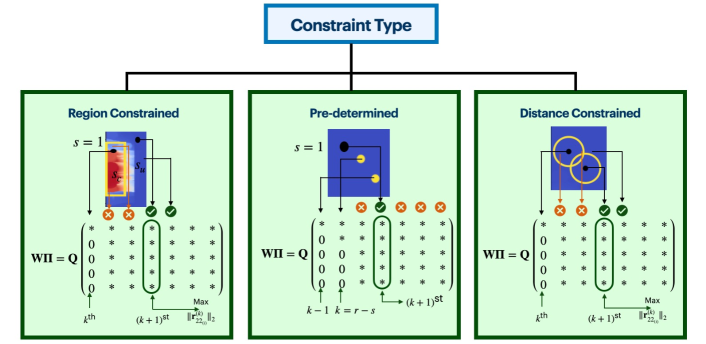
Figure 2: Greedy selection of the next sensor involves choosing the next pivot column of $\mathbf{\Psi}^{T}$ from the set of allowable sensor locations specified by the constraint.

Consider the following partial QR factorization at the $k^{\text{th}}$ iteration in the pivoting procedure:

$$\mathbf{W}\mathbf{\Pi}=\mathbf{Q}\mathbf{R}=\mathbf{Q}\begin{bmatrix}\mathbf{R}_{11}^{(k)}&\mathbf{R}_{12}^{(k)}\\ {0}&\mathbf{R}_{22}^{(k)}\end{bmatrix},$$ (11)

where $\mathbf{Q}\in\mathbb{R}^{m\times m}$ is orthogonal, $\mathbf{R}_{11}^{(k)}\in\mathbb{R}^{k\times k}$ is upper triangular, $\mathbf{R}_{12}^{(k)}\in\mathbb{R}^{k\times(n-k)}$, $\mathbf{R}_{22}^{(k)}\in\mathbb{R}^{(m-k)\times(n-k)}$, and $\mathbf{\Pi}\in\mathbb{R}^{n\times n}$ is the permutation matrix containing information about the first $k$ chosen sensors [55, 56, 57]. In unconstrained QR pivoting, the $(k+1)^{\text{st}}$ iteration selects a column from the submatrix $\mathbf{R}_{22}^{(k)}$ with the maximal two-norm, then swaps the selected column with the $(k+1)^{\text{st}}$ column while updating permutation indices

$$l=\operatorname*{argmax}_{i=1,\ldots,n-k}\|\mathbf{r}_{22_{(i)}}^{(k)}\|_{2}.$$ (12)

Constraints are integrated within this step, by forcing the pivot column index to be selected from the latest set of allowable indices based on the constraints under consideration. The $k+1^{\text{st}}$ iteration in constrained optimization selects the pivot column with largest 2 norm, $\mathbf{r}_{22_{(i)}}^{(k)}$, from the constrained/unconstrained set of allowable column indices in $\mathbf{R}_{22}^{(k)}$. The QR pivoting algorithm results in the following diagonal dominance structure in $\mathbf{R}$:

$$|\mathbf{R}_{ii}|^{2}\geq\sum_{j=1}^{k}|\mathbf{R}_{jk}|^{2},\,\,1\leq i\leq k\leq r.$$ (13)

Constraints are imposed in the final $r-s$ steps of pivoting, ensuring that the largest contributing terms in the objective function expansion remained unaffected:

$$\log\det((\mathbb{S}\boldsymbol{\Psi_{r}})^{T}\mathbb{S}\boldsymbol{\Psi_{r}}) =\log\left(\prod_{i=1}^{r}\mathbf{R}_{ii}^{2}\right)$$ (14)

$$=\log\mathbf{R}_{11}^{2}+\log\mathbf{R}_{22}^{2}+\dots+\log\mathbf{R}_{(r-s)(r-s)}^{2}+\dots+\log\mathbf{R}_{rr}^{2}.$$

The main driver of this optimization is the point at which constraints are introduced into the pivoting procedure, as allowing upper triangularization to proceed normally in the starting iterations maximizes the leading diagonal entries of $\mathbf{R}$, ensuring that domain-specific constraints do not drastically affect the diagonal dominance property, but only the trailing $\mathbf{R}_{ii}$, which are optimized by choosing the best pivot from the allowable locations. The three types of spatial constraints handled by the algorithm (Figure 2) are:

1. Region constrained: This type of constraint arises when we can place either a maximum of or exactly $s$ sensors in a certain region, while the remaining $r-s$ sensors must be placed outside the constraint region.

   Maximum: This case deals with applications in which the number of sensors in the constraint region should be less than or equal to $s$. In each iteration a pivot column (sensor location) is chosen from the set of all columns until $s$ selected pivots lie in the constrained region. Successive pivots with the largest 2-norm are selected from among the unconstrained column indices.

   Exact: This case deals with applications in which the number of sensors in the constraint region should equal $s$. The algorithm follows the same procedure as the maximum sensor placement case if the number of sensors in the constraint region equals or exceeds $s$. However, if there are fewer than $s$ sensors in the constrained region, the algorithm forces the deficit of sensors to be placed in the constraint region at the end of the pivoting procedure.

2. Predetermined: This type of constraint occurs when a certain number of sensor locations are already specified, and optimized locations for the remaining sensors are desired. The strategy employed selects pivots from among all column indices of $\mathbf{R}_{22}^{(k)}$ until the iterate $k$ equals $r-s$, then imposes the selection of user-specified sensor locations in the final $s$ iterations.

3. Distance constrained: This constraint enforces sensors to be placed a specified distance $d$ apart. Accordingly, the first pivot is the column index of $\mathbf{\Psi}_{r}^{T}$ with maximal 2-norm, the default (unconstrained) base step. The $(k+1)^{\text{st}}$ iterate now selects the pivot column with maximal 2-norm from among the remaining columns of $\mathbf{R}_{22}^{(k)}$ that are at least distance $d$ away from the previous $k$ selected sensors. This is an adaptive constraint because the set of allowable sensor indices is updated with each pivoting iteration to remove the $d$-neighborhood of the $k$th sensor.

Although we mainly consider the minimal allowable number of sensors to be $p=r$, the truncation rank of the basis, additional sensors can be added for redundancy and robustness through the oversampling optimization proposed by B. Peherstorfer et al [58].

3.3 Uncertainty analysis

Under noisy measurements, errors in estimation are transmitted into reconstruction errors. Geometrically, estimation errors are characterized by (hyper-)ellipsoids in $r$ dimensions whose axes describe these errors. Statistically, the confidence intervals for the estimation of states are characterized by the $\eta$-confidence ellipsoid that contains $\mathbf{a}-\mathbf{\hat{a}}$ with probability $\eta$

$$E_{\alpha}=\{\mathbf{z}|\mathbf{z}^{T}\boldsymbol{\Sigma}^{-1}\mathbf{z}\leq\alpha\},$$ (15)

where $\mathbf{\Sigma}$ is the covariance matrix in Equation 8 and $\alpha=F_{\chi_{n}^{2}}^{-1}(\eta)$ is the cumulative distribution function of a $\chi$-squared random variable with $r$ degrees of freedom. One of the scalar measures for quality of estimation is the volume of this ellipsoid

$$\textbf{vol}(\epsilon_{\alpha})=\frac{(\alpha\pi)^{r/2}}{\Gamma(\frac{r}{(2+1)})}\det\boldsymbol{\Sigma}^{1/2}=\frac{(\alpha\pi)^{r/2}}{\Gamma(\frac{r}{(2+1)})}\det((\beta^{2}((\mathbb{S}\mathbf{\Psi}_{r})^{T}(\mathbb{S}\mathbf{\Psi}_{r}))^{-1})^{1/2}),$$ (16)

where $\Gamma$ is the gamma function. D-optimal designs minimize the volume of the ellipsoid, as the volume of the ellipsoid is inversely proportional to the determinant of our information matrix. A small volume for the $\eta$-confidence ellipsoid implies a strong correlation between the estimation errors in each component. Under Gaussian noise assumptions, $3\sigma$ standard deviations computed from the diagonal entries of the covariance matrix $\Sigma_{ii}$ measure the uncertainty in predicting the $i^{th}$ component, establishing error bounds for reconstructing flows from noisy measuremetns. In nuclear digital twins these error bounds can be used to detect the divergence of sensor readings from expected values. Statistics of the error provide means to “flag” or “signal” re-calibration of the digital twin, detect anomalies and classify erroneous readings.

Algorithm 1 QR Pivoting with Adaptive Constraints

1:Input: $\mathbf{W}$ = Input matrix, $s_{c}$ = Constrained/Predetermined sensor indices, $s$ = indices allowed in the constrained region/ Total predetermined sensors, CONSTRAINTS = Type of Constraint, $d$ = Distance from previous sensors

2:Output: Sensor indices

3:Function Call: $\gamma$ = CONSTRAINEDQR($\Psi_{r}^{T}$, CONSTRAINTS, $s_{c}$=[], $s$=[], $d$=2)

4:procedure constrainedQR($\mathbf{W}$, Constraints,$s_{c}$,$s$,$d$)

5:     $r,n\leftarrow$Size($\mathbf{W}$) $\triangleright$ $r$ = number of desired sensors

6:     $\mathbf{R}\leftarrow$Copy($\mathbf{W}$)

7:     $\mathbf{Q}\leftarrow eye(m)$

8:     $\gamma\leftarrow[1,2,\dots,n]$ $\triangleright$ Permutation (sensor) index set

9:     for all $k\in 1,....,r$ do

10:         $dlens\leftarrow$ computeConstraints($dlens$,$\gamma$,CONSTRAINTS,$k$,$s_{c}$,$s$,$d$)

11:         $l\leftarrow\operatorname*{argmax}dlens$

12:         $\boldsymbol{\nu}\leftarrow\mathbf{R}[k:m,k-1+l]$

13:         swap($\mathbf{R}[k:m,k],\mathbf{R}[k:m,k-1+l]$)

14:         swap($\gamma_{k},\gamma_{k-1+l}$) $\triangleright$ Update $k$th sensor

15:         $u\leftarrow\textsc{Householder}(\boldsymbol{\nu})$ $\triangleright$ Householder reflector $H(\nu)$

16:         $\mathbf{R}[k:m,k:n]\leftarrow(I-2uu^{T})\mathbf{R}[k:m,k:n]$ $\triangleright$ Apply Householder projection

17:         $\mathbf{Q}[:,k:n]\leftarrow(I-2uu^{T})\mathbf{Q}[:,k:n]$      

18:     return $\gamma_{1:r}$

Algorithm 2 Subroutine for Constraints

1:Input: $s_{c},s,r,d$, CONSTRAINTS = as mentioned in 1, $dlens$ = Norm of each column of $\mathbf{R}$, $\gamma$ = Permutation (sensor) index set, $k$ = Current sensor index

2:Output: Updated $dlens$

3:procedure computeConstraints($dlens$,$\gamma$,Constraints,$k$,$s_{c}$,$s$,$r$,$d$)

4:     if CONSTRAINTS = RegionConstrainedMax then

5:         if $|\gamma|\in s_{c}<s$ then $\triangleright$ Number of sensors in constrained region less than $s$

6:              $dlens$ = $dlens$

7:         else$\triangleright$ Number of sensors in constrained region $\geq s$

8:              $dlens[s_{c}]=0$          

9:     else if CONSTRAINTS = RegionConstrainedExact then

10:         if $|\gamma|\in s_{c}<s$ then $\triangleright$ Number of sensors in constrained region $<s$

11:              $dlens$ = $dlens$

12:              if $r>k\geq(r-(s-|\gamma|)$ then $\triangleright$ We want exactly s in constrained region

13:                  $dlens[!s_{c}]=0$               

14:         else$\triangleright$ Number of sensors in constrained region $>s$

15:              $dlens[s_{c}]=0$          

16:     else if CONSTRAINTS = Pre-determined then

17:         if $k=(r-s)$ then $\triangleright$ $(r-s)$ sensors have already been placed

18:              $dlens[!s_{c}]$ = 0 $\triangleright$ Place pre-determined sensors at the end          

19:     else CONSTRAINTS = DistanceConstrained

20:         if $p\in dlens$ and $\|p-\gamma[:]\|_{2}\leq d$ then $\triangleright$ All sensor locations within $d$ (2-norm distance)

21:              $dlens[p]=0$               

4 Results

This section demonstrates the constrained and unconstrained sensor placement algorithm on a randomly generated state space system, the 2D heat diffusion through a thin plate, and the OPTI-TWIST prototype. In the randomized system, all possible sensor placements given a fixed budget of sensors are computed to demonstrate the near optimality of our approach. Next, we investigate reconstruction of temperature fields in 2D heat diffusion with a constant heat source, a simplified model of the OPTI-TWIST heater. Uncertainty analysis is conducted on noisy measurements for varying signal-to-noise ratio (SNR). Using constrained optimized sensor placement with our approach, we reconstruct, with minimal error, the flow field inside OPTI-TWIST—in comparison to randomly selected sensor locations.

4.1 Discrete random state space

We first demonstrate the near optimality of constrained QR pivoting by using a low-dimensional linear time-invariant (LTI) system. The dimensionality of this system is small enough to enumerate all possible placements in order to empirically compare the constrained QR placements with the optimum placements. Consider the following LTI system:

$$\dot{\mathbf{x}} =\mathbf{A}\mathbf{x}+\mathbf{B}\mathbf{u} \mathbf{x}\in\mathbb{R}^{n},\mathbf{u}\in\mathbb{R}^{q}$$ (17a)

$$\mathbf{y} =\mathbf{C}\mathbf{x} \mathbf{y}\in\mathbb{R}^{p}$$ (17b)

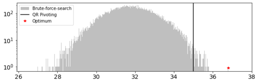
(a) Unconstrained QR pivoting

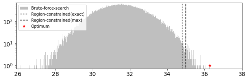
(b) Region-constrained QR pivoting

\begin{overpic}[scale={.47},percent]{Figures/Figure3cHistogramPredetermined.pdf} \put(-3.0,38.0){\rotatebox{90.0}{Number of Placements}} \put(37.0,-1.0){$\log\det(\mathbb{S}\boldsymbol{\Psi_{r}})^{T}(\mathbb{S}\boldsymbol{\Psi_{r}})$} \end{overpic}

(c) User-specified QR pivoting

Figure 3: Enumeration of $\log\det(\mathbb{S}\boldsymbol{\Psi_{r}})^{T}(\mathbb{S}\boldsymbol{\Psi_{r}})$ over all possible placements of 7 out of 25 candidate locations (100,000-500,000 possible placements binned into histograms). The introduction of constraints into QR optimization results in a log determinant that is near optimal (optimum shown in red) for the three types of constraints.

with randomly generated system $\mathbf{A}$, measurement $\mathbf{C}$, and actuation $\mathbf{B}$ matrices sampled i.i.d. from a normal distribution, $n=25$ states and $p=q=25$ randomized measurements and actuators, respectively. $\mathbf{x}$, $\mathbf{u}$, and $\mathbf{y}$ represent the state, input, and output vectors, respectively. We empirically studied the optimality of our proposed algorithm by computing all possible $r=7$ sensor selections, leading to a brute force search of ${n\choose r}=480,700$ choices of $\mathbb{S}$. The log determinant of $\mathbb{S}\boldsymbol{\Psi_{r}}$ was evaluated for all possible combinations of the seven sensors, then binned into the histogram shown in 3(a). This computation is only tractable for a small state dimension—as even for $n=100$, the brute-force search results in $O(10^{10})$ complexity. The optimization outcome (determined via Equation 9) for sensors selected using the QR pivoting approach is represented by the solid black line in 3(a). This sensor selection is observed to be nearly D-optimal, exceeding 99.74% of all candidate placements.

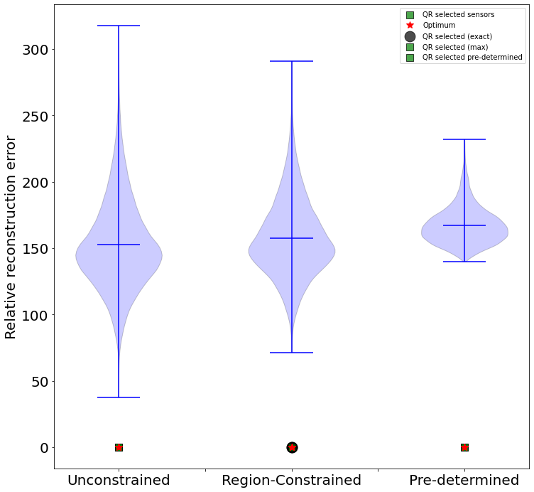
Figure 4: Reconstruction error comparison. Proximity between the brute-force optimum and QR selected sensors for unconstrained, region-constrained, and predetermined sensor placement leads to orders of magnitude lower reconstruction error ($\epsilon\sim\mathcal{O}(10^{-15})$) compared to random placements. Incorporating constraints results in accuracy comparable to that of the optimal placement (red stars).

We studied region-constrained pivoting by allowing only $s\leq 2$ sensors to be selected from the first $s_{c}=5$ components of the state (the constraint region). A brute-force search across all possible combinations of $s$ sensors in the constraint region (and $r-s$ elsewhere) was carried out, resulting in $\frac{(n-s_{c})!}{(n-s_{c}-(r-s))!(r-s)!}\frac{s_{c}!}{(s_{c}-s)!s!}=155,040$ possible combinations in selecting the seven sensors binned in 3(b). 3(b) compared our first strategy (i.e., placing exactly $s=2$ sensors in the constraint region in the first two iterations of pivoting (dotted line)) with another strategy in which a maximum of two sensors were allowed in the constraint region throughout the pivoting procedure (dashed line). Our exact approach has a log determinant exceeding 99.78% of all possible region-constrained sensor placement options, while the max approach is observed to exceed 99.87% of all possible combinations. Thus, both approaches provide a near-optimal subset of region-constrained sensors for reconstruction.

In predetermined sensor placement, a specified number $s$ of sensors were selected in advance, leaving the algorithm to optimize those that remain. Our strategy runs unconstrained QR pivoting to select the first $r-s$ pivots (sensors), then selects the predetermined sensors in the remaining $s$ pivoting iterations. The results of the log determinant objective evaluated for our optimization strategy (dashed line) are compared against a brute force search across all possible candidate placements that contain the two predetermined sensors reflected in 3(c). Our strategy outperforms 99.99% of all possible placements, exhibiting near-optimal solutions.

These results show that the introduction of constraints results in minimal distance to the true optimum. We analyze the negligible effect of this distance on the reconstruction error

$$\text{Relative reconstruction error}(\epsilon)=\frac{\|\mathbf{x}-\mathbf{\Psi}_{r}(\mathbb{S}\mathbf{\Psi}_{r})^{\dagger}\mathbf{y}\|_{2}}{\|\mathbf{x}\|_{2}}\times 100.$$ (18)

We compared the reconstruction achieved via each set of constrained QR sensors with sensor placements sampled from the mean of the $\log\det$ distributions. (These represent the most likely sub-optimal sets to be chosen at random.) The reconstruction error for each of these randomly placed sensors was then calculated (see the blue violin plots in Figure 4, where the green square and circle reflect the reconstruction error of the QR-selected sensor locations for the different constraint cases). Random sensor placements with a sub-optimal $\log\det$ objective fall between 31 and 32, resulting in a highly inaccurate relative reconstruction error $(\epsilon)$ between 30 and 350. The QR-optimized strategy for unconstrained/constrained sensor placement results in significantly lower reconstruction error $\epsilon\sim\mathcal{O}(10^{-15})$:

We conclude that the proximity between the brute-force optimum and our greedy placements produces negligible loss in reconstruction performance. Vastly sub-optimal random placements illustrate the inverse relationship between the objective function and performance: the lower the log determinant, the higher the reconstruction error. However, this system was randomly generated, and the dynamics do not evolve according to localized features in state space that allow one sensor to capture information on spatially correlated states. Next, we demonstrate the algorithm on a heat diffusion model that allows for spatial and physical interpretation of the resulting sensors.

4.2 2D heat flow through a thin plate

Temperature fields are reconstructed via constrained/unconstrained sensor placement in a 2D plate undergoing thermal diffusion from a heat source, based on a simplified model of the OPTI-TWIST diffusion. Temperatures at the boundaries are fixed at $100\degree C$ at $x=0$, and $36\degree C$ elsewhere in $\partial D$. The initial temperature throughout the domain $D$ at $t=0$ is also $36\degree C$ (as seen in 5(a)). Heat transfer from the heat source to the rest of the domain is governed by the heat equation

$$u_{t}=\alpha(u_{xx}+u_{yy})$$ in D

$$u(x,y,t)=36 x,y\in\partial D\setminus x=0$$

$$u(0,y,t)=100$$

\begin{overpic}[scale={.37},percent]{Figures/heatplate1.pdf} \put(45.0,33.0){D} \end{overpic}

(a) Initial conditions

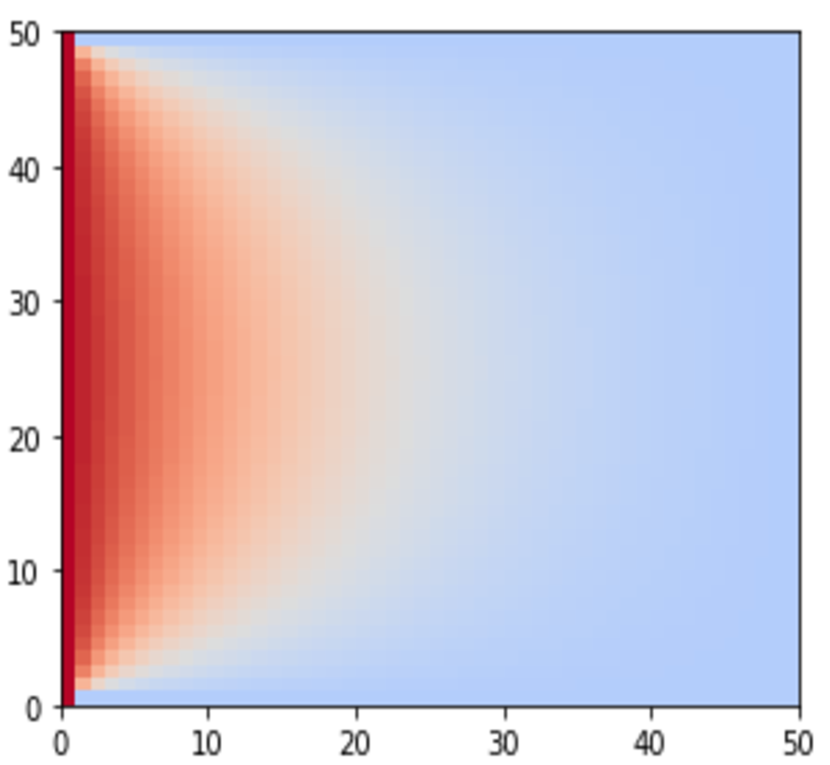
(b) Truth

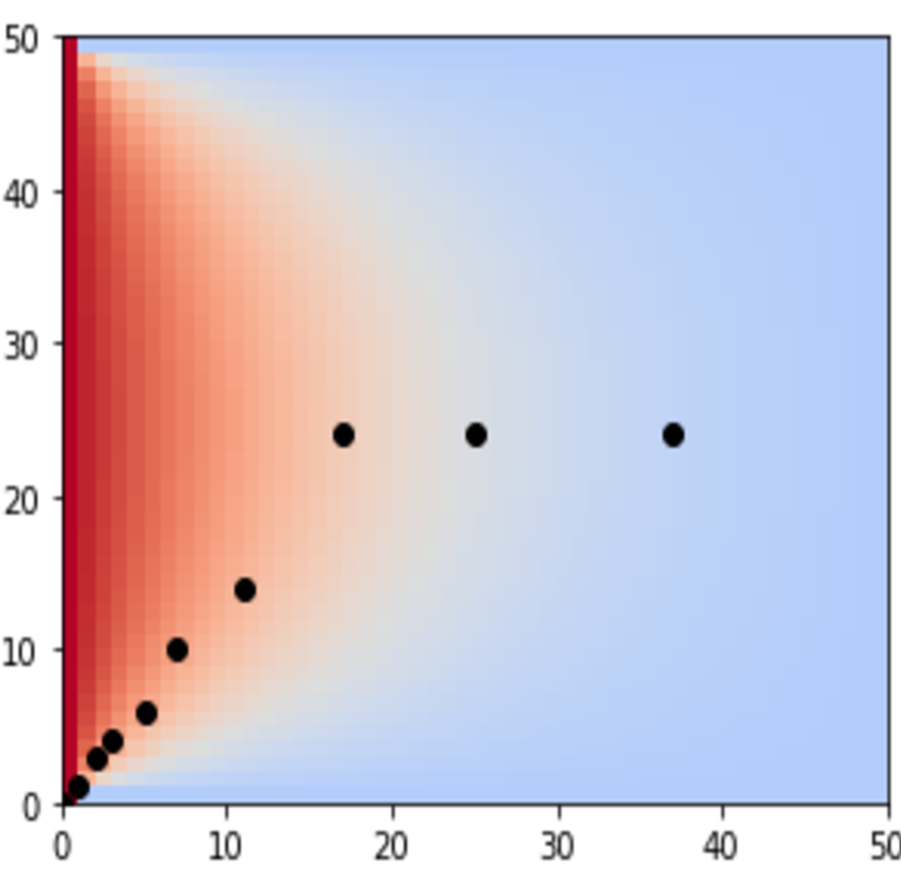
(c) QR $\epsilon$ = 0.0064

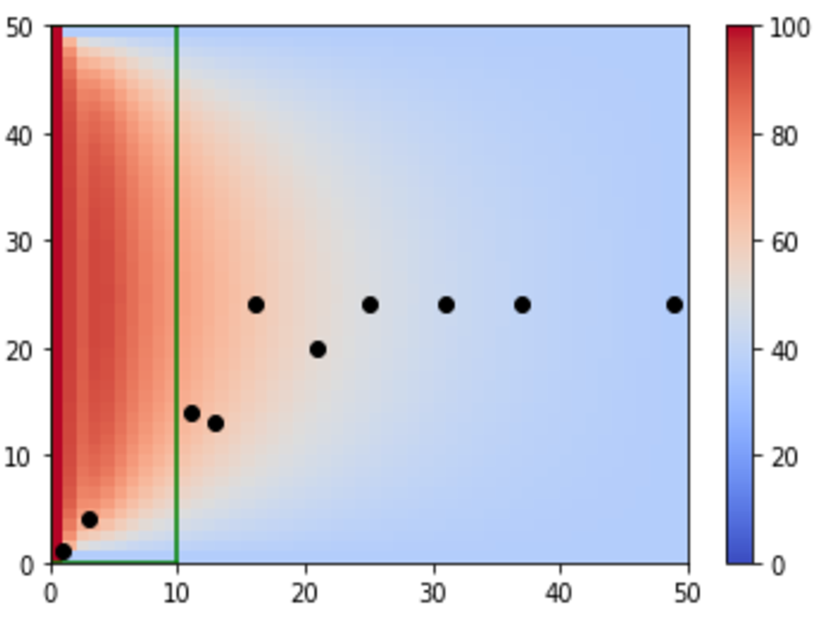
(d) Exact $\epsilon$ = 1.5085

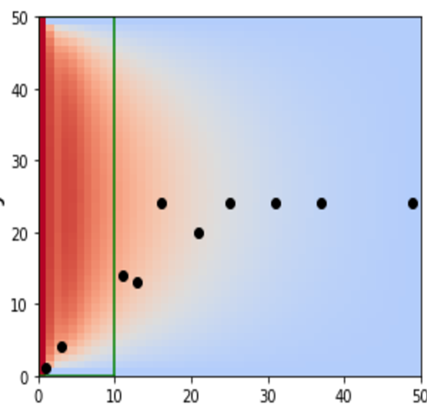
(e) Max $\epsilon$ = 1.5085

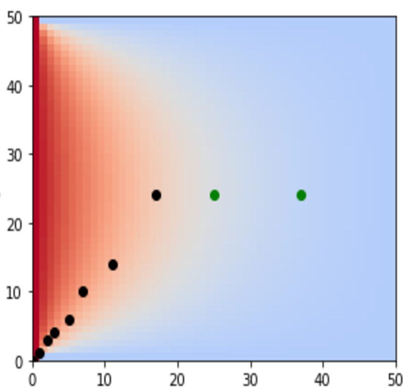
(f) Pre $\epsilon$ = 0.0127

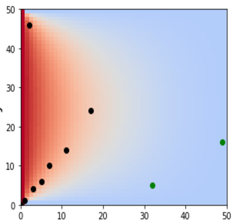
(g) Pre $\epsilon$ = 0.0111

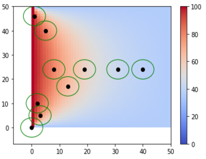
(h) Distance $\epsilon$ = 0.0103

Figure 5: Reconstruction of the temperature field through selected sensors. Reconstruction of the temperature field at $t=1000$, based on the types of constraints implemented in subsection 3.2 (d-h, shown in green) demonstrate that constraining sensors far away from the heater region result in higher reconstruction error than unconstrained optimization (c), which favors sensors adjacent to the heat source.

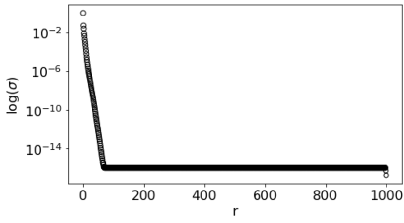
(a) Energy content

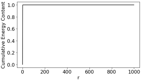
(b) Cumulative energy content

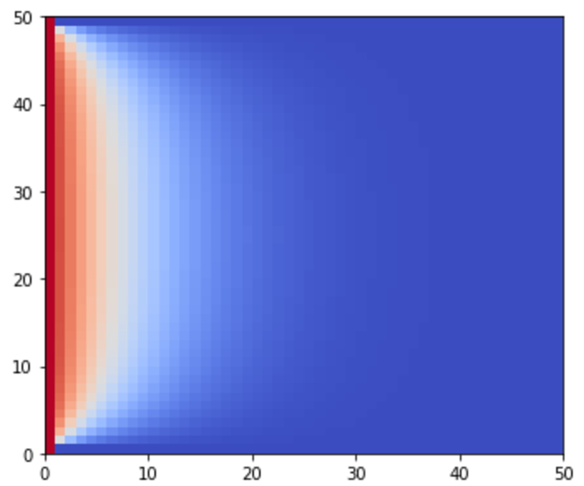
(c) $\sigma_{1}$ = 0.9152

(d) $\sigma_{2}$ = 0.0525

(e) $\sigma_{3}$ = 0.0244

(f) $\sigma_{4}$ = 0.0011

Figure 6: Leading POD modes by energy contribution. The leading two modes of the heat diffusion capture $96\%$ of the energy in the dynamics. Higher-energy modes are concentrated near the heat source at $x=0$.

where $u$ is the desired temperature and $\alpha=2\,(\text{mm}^{2}/\text{s}$) is the thermal diffusivity constant. The solution of the partial differential equation is simulated for 1000 time steps using finite differences with $\Delta x,\Delta y=1$ and $\Delta t=0.125$. We reconstruct the temperature fields for the unconstrained, constrained, and predetermined optimized sensor placements reflected in Figure 5. A total of $r=10$ sensors are selected for reconstruction, and $s=2$ sensors are allowed in the constrained region or are predetermined. Distance constraints impose a Euclidean distance of at least 2 between selected sensors.

Similar to the nuclear OPTI-TWIST (subsection 4.3), optimized placements favor sensors near the heat source. Constraining sensors away from the heat source results in higher reconstruction errors than unconstrained optimization. In this example, both region-constrained max and exact ($s=2$ within $x<10$) optimization result in identical sensor placements (5(d), 5(e)), with only two sensors near the heat source. This results in higher error because of high-energy modal contributions adjacent to the heater (Figure 6). The predetermined and distance-constrained sensor placements, which also placed six sensors near the heat source, result in the lowest reconstruction error under constraints (5(f), 5(g), 5(h)).

The optimized sensors reflect the highest energy amplification in the POD modes, which occur near the heat source (Figure 6). The leading POD modes capture this diffusion of heat from the heat source boundary to the rest of the domain (6(b)). Approximately 96% of the cumulative energy is captured by the $1^{st}$ two POD modes, while the remainder capture only 4%.

\begin{overpic}[scale={.5},percent]{Figures/Figure7HeatErrors.pdf} \put(-2.5,10.0){\rotatebox{90.0}{$\mathbf{a}_{1}-\hat{\mathbf{a}}_{1}$}} \put(39.0,-2.0){Time-step/Samples} \end{overpic}

Figure 7: Estimation error bounds under noisy measurements. $3\sigma$ bounds (dotted green) for the estimation error of $\mathbf{a}_{1}$ (blue) effectively bound the estimation error for snapshots closer to the training time interval. The inability of the POD to capture translating modes outside training data is reflected in the final snapshots, as the temperature diffuses towards the right boundary. Such deviations can be used to retrain digital twin models.

\begin{overpic}[scale={.38},percent]{Figures/Fig5bbounds.pdf} \put(-2.5,40.0){\rotatebox{90.0}{$\mathbf{a}_{k}-\hat{\mathbf{a}}_{k}$}} \put(53.0,-2.0){$r$} \end{overpic}

(a) Decrease in $\mathbf{a}_{k}-\hat{\mathbf{a}}_{k}$ with an increase in sensors.

\begin{overpic}[scale={.39},percent]{Figures/Figure8bSNR.pdf} \put(-2.0,40.0){\rotatebox{90.0}{$\mathbf{a}_{k}-\hat{\mathbf{a}}_{k}$}} \put(50.0,-3.3){SNR} \end{overpic}

(b) Increase in $\mathbf{a}_{k}-\hat{\mathbf{a}}_{k}$ with a decreasing SNR.

Figure 8: Uncertainty analysis. The estimation error in the components of $\mathbf{a}$ due to noisy measurements is bounded by three standard deviations for increasing number of sensors (left) and increasing noise (right).

Next, we study the uncertainty in the reconstruction from noise-corrupted sensor measurements by adding i.i.d.Gaussian noise $\boldsymbol{\eta}\sim\mathcal{N}(0,0.001)$ to the measurements. Gappy POD was used to estimate the first $r=20$ POD coefficients from these noisy measurements (test dataset of 500 snapshots), and compare the resulting reconstruction error with the ground truth. The standard deviations $\sigma_{i}$ computed from the diagonal entries of the covariance matrix $\mathbf{\Sigma}_{ii}$ measures the uncertainty in predicting the $i$th component. $99.7\%$ of reconstructed errors should lie within three standard deviations or $3\sigma_{i}$ of the mean (Figure 7) (approximately 498.5 out of 500 reconstruction errors). As more modes are included in the POD approximation, the sensor selection algorithm captures more information about the underlying physics of heat diffusion. Therefore, a higher number of sensors leads to a lower reconstruction error. With more modes and sensors, the error covariance in each component narrows to $3\sigma_{i}\approx$ 1e-10, as shown in 8(a). Similarly, as the SNR decreases, the dynamics of heat diffusion are corrupted by noise, resulting in an increasing state estimation error (8(b)).

In summary, when the noise distribution is known, this framework enables estimation of the expected error distribution as a function of measurement noise, as well as study of the growth in error as the sensor noise increases. When the noise distributions are unknown, filtering and Bayesian inference techniques may be used for uncertainty quantification. The developed algorithm can handle reconstruction of flow fields in the presence of constraints and noise with high accuracy. Uncertainty analysis of predicted states plays a key role in detecting erroneous readings in digital twins. In the next example we reconstruct temperature flow field for a gravitational advection driven physical system, OPTI-TWIST.

4.3 Steady-state simulation of the OPTI-TWIST prototype

The next example follows the new design paradigm suggested by digital twins. In traditional design practice, modeling and simulation insights are often leveraged at the experimental design stage in order to build physical models and place sensors. However, limitations regarding space, installation, cost, and signal fidelity of the experimental device pose challenges in deploying the desired number of sensors. Our holistic approach integrates experimental constraints, Computational Fluid Dynamics (CFD) simulations, and optimization objectives (reconstruction) in a principled way to optimize the placement of sensors. This occurs in the design phase of the digital twin, when the digital twin prototype is being configured to realize the physical instance once it is up and running.

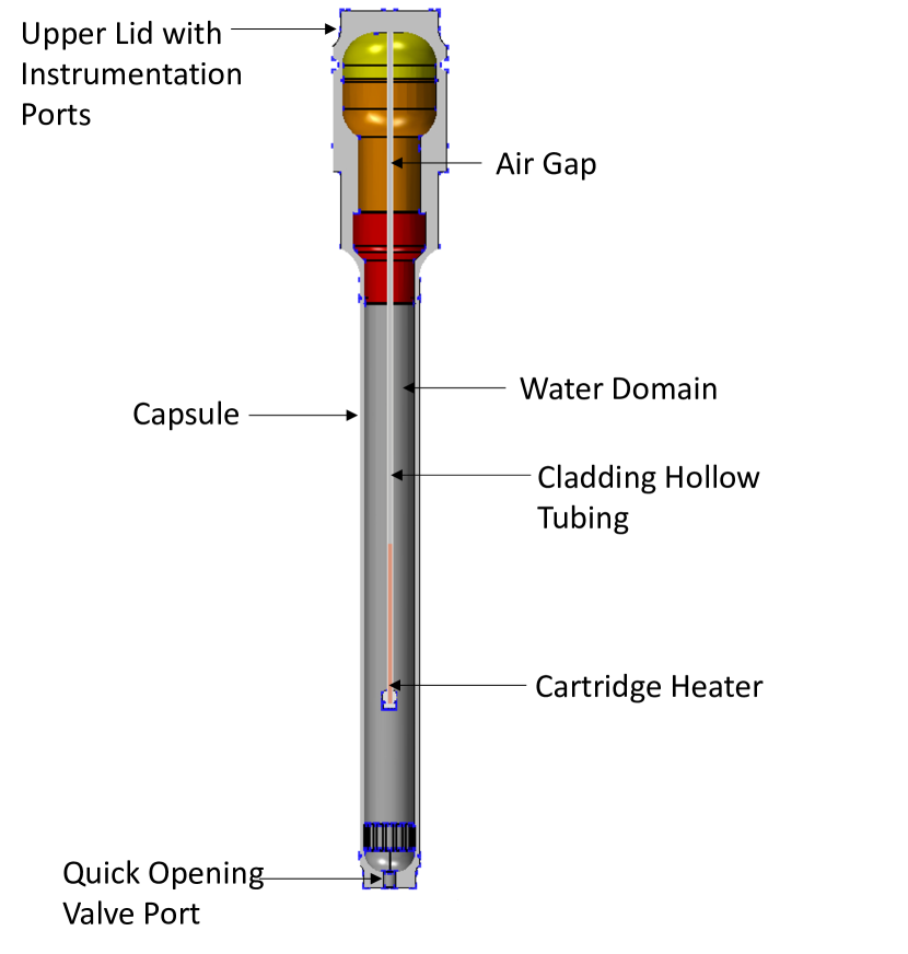
(a) Schematic

\begin{overpic}[scale={.4},percent]{Figures/Figure9Twistmesh.pdf} \put(40.0,73.0){Heat Source} \put(40.0,43.0){Heater Region} \end{overpic}

(b) Mesh

Figure 9: Geometry and mesh of OPTI-TWIST. The CAD model of OPTI-TWIST centers the cartridge heater in the capsule, exploiting its axial symmetry to simulate only half the domain, i.e. the central axis of the cartridge heater and the capsule outer wall define the domain boundaries. The heat source is embedded within the heater domain, and the surface temperature was applied as a boundary condition on the external surface of the OPTI-TWIST capsule.

Here, our sensor placement optimization is demonstrated on the OPTI-TWIST prototype, which is electronically heated to mimic the neutronics effect of TWIST prior to insertion into a reactor at INL. Temperature is the field of interest in this case, and point thermocouples will be used as the sensors. The OPTI-TWIST prototype was designed to simulate thermal-hydraulics behavior of TWIST during irradiation in the reactor, as well as to measure the effect of loss of coolant on the fuel rodlet temperature. In OPTI-TWIST, the fuel-rod specimen is replaced by an instrumented electric cartridge heater, and loss of coolant is controlled by a quick-opening valve at the bottom of the capsule. To provide the temperature fields necessary to train the sparse sensing algorithm, a 2D CFD model reflecting a simplified version of the OPTI-TWIST geometry was developed and analyzed using StarCCM+ (Figure 9) [59]. The CFD model accounts for steady-state turbulent natural circulation conditions, including two controlled parameters: heater power ($\dot{q}$) and outer surface temperature ($T_{sur}$).

These two controlled parameters (i.e., heater power and surface temperature) were varied, while keeping the initial temperatures ($T_{0}=300$ K) and the system pressure ($P_{sys}=2250$ psi) constant throughout. The data are comprised of 49 steady-state temperature fields resulting from seven heater powers and surface temperatures uniformly sampled at 350–650 W and 240–420 K, respectively. The convergence criterion was the maximum liquid temperature, which showed minimal fluctuations after 2000 time steps.

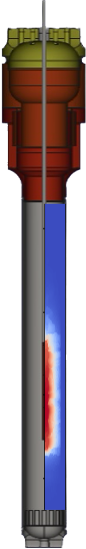
\begin{overpic}[scale={.56},percent]{Figures/Figure9cTwistRandom.pdf} \put(-2.5,34.0){\rotatebox{90.0}{Height [cm]}} \end{overpic}

(a) Random

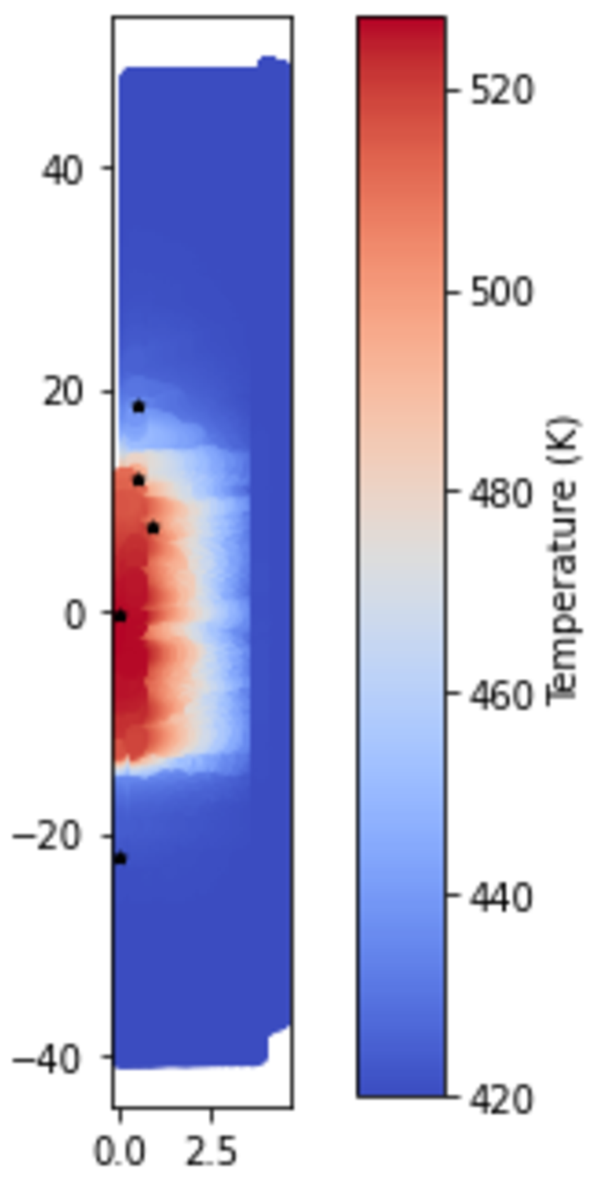
(b) Optimal

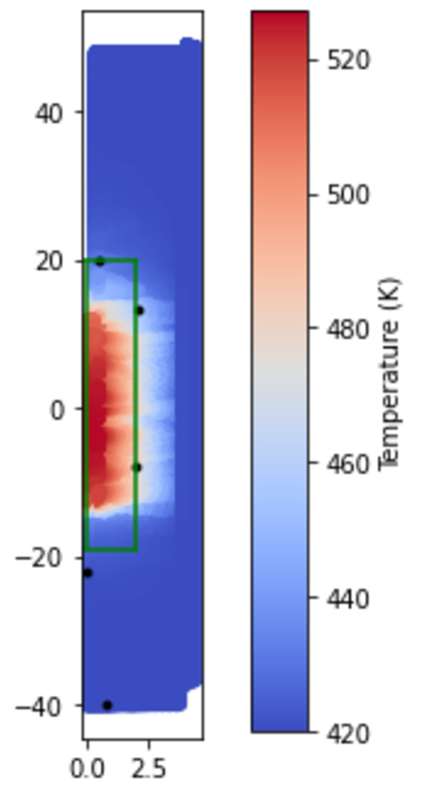
(c) Constrained optimal

Figure 10: OPTI-TWIST model (left) and sensor placements superimposed on reconstructions. Although unconstrained optimization places sensors near the heat source (b), constraints on sensor installation are imposed within our optimization procedure, resulting in the placement of sensors outside the depicted region (c). Note that random placement results in inaccurate reconstruction.

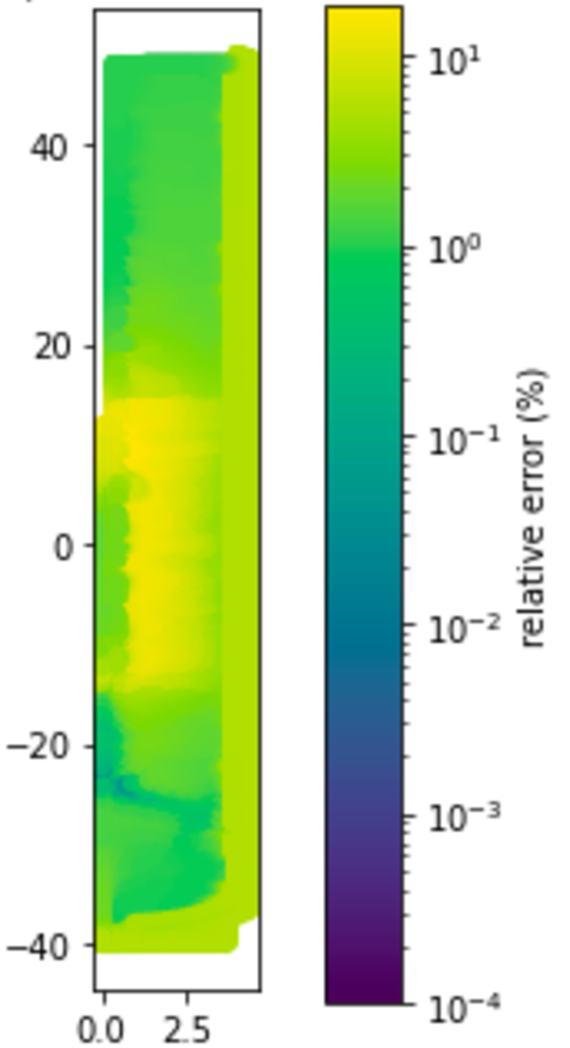
(a) Random $\epsilon=25.24$

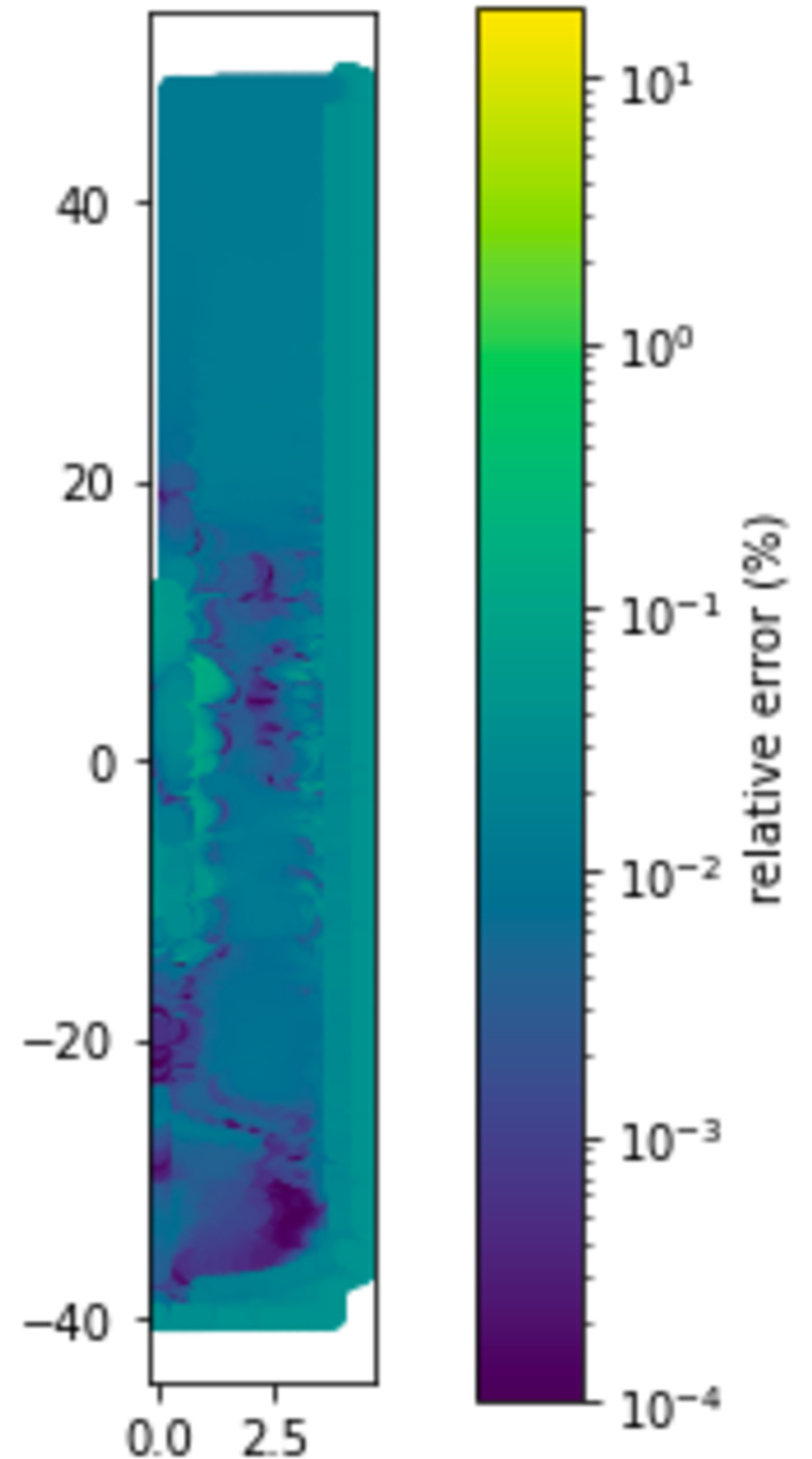
(b) Optimal $\epsilon=0.168$

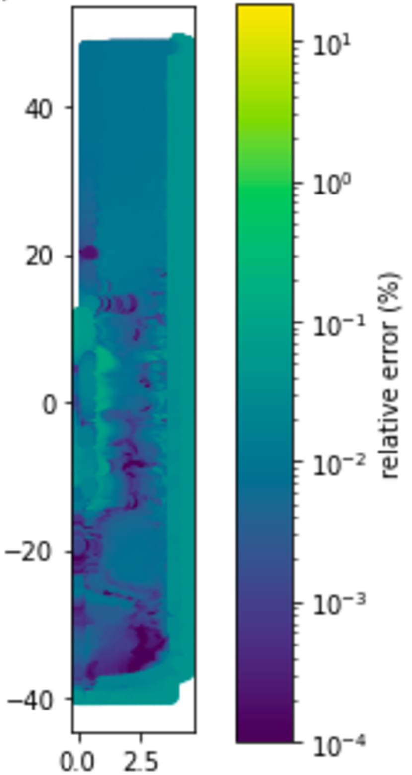
(c) Constraints $\epsilon=0.174$

Figure 11: OPTI-TWIST reconstruction error. The relative reconstruction error ($\epsilon$) for QR-selected sensor locations is much lower $(\mathcal{O}(10^{-1}))$ than reconstruction with sensors placed at random locations.

Sensor Placement	Optimization Objective	Reconstruction Error ($\epsilon$)
Unconstrained	5.432829081027846e-10	0.168
Constrained	4.534195929074569e-11	0.174
Random	1.026196077627373e-12	25.24

Table 2: Summary of the relative reconstruction error ($\epsilon$) and optimization criteria ($\log|\det\mathbb{S}\boldsymbol{\Psi_{r}}|$) for sensor placement given in Figure 11.

First, our optimization is run on the steady-state temperature fields, resulting in the unconstrained optimal placement shown in 10(b). Unconstrained optimization selects three sensors near the heater (10(b)); however, space restrictions make these heater-adjacent locations experimentally infeasible. Enforcing sensor constraints to lie outside the heater region results in a reconstruction error of $\epsilon=0.174$—an increase of only .006. 10(a) contrasts these optimized sensor reconstructions with ensembles of randomly placed sensors. Observe that $\epsilon_{unconstrained}<\epsilon_{constrained}\ll\epsilon_{random}$, i.e. placing sensors in random locations leads to significantly larger reconstruction errors (Table 2).

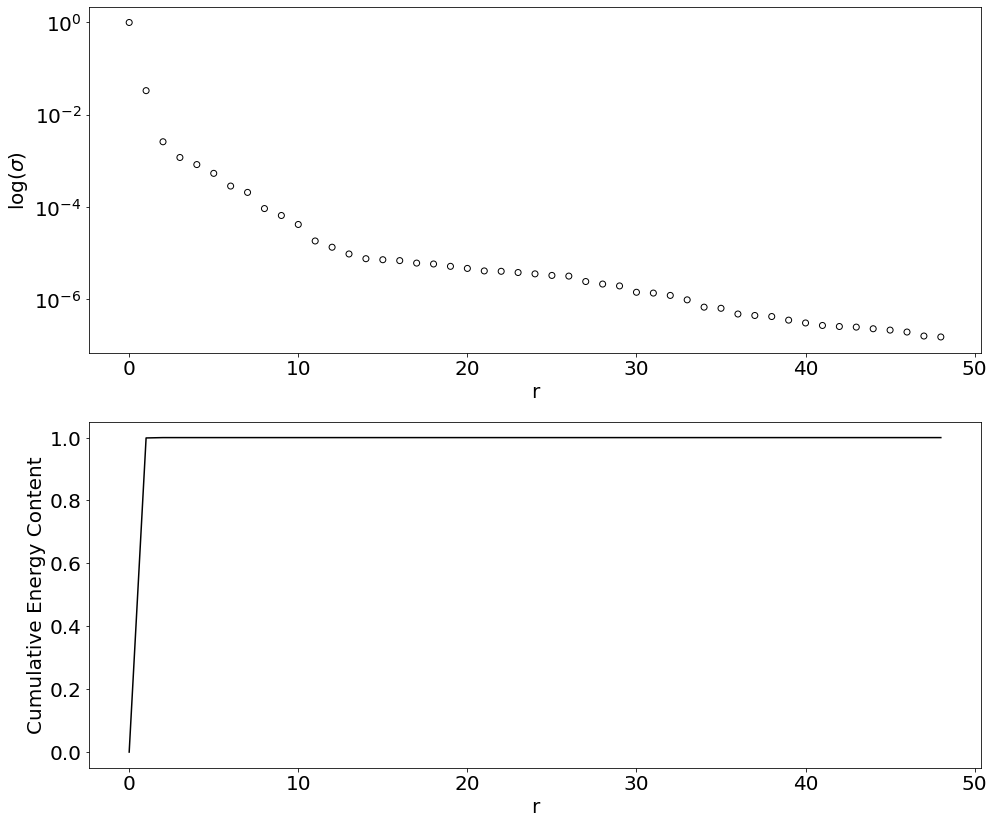
(a) Cumulative energy content of normalized singular values ($\sigma$)

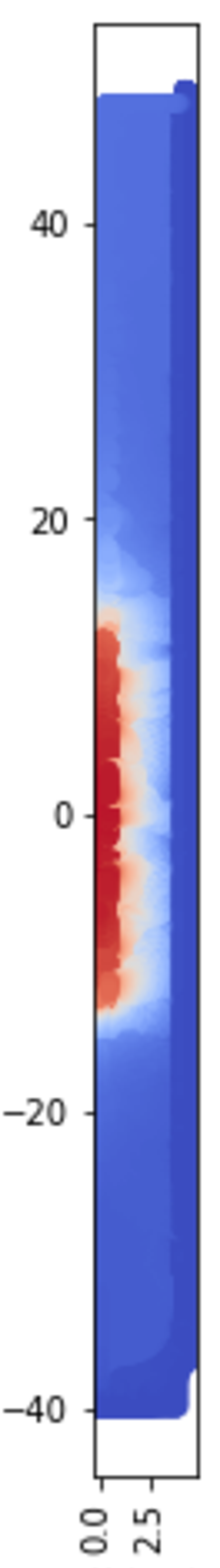
(b) $\sigma_{1}=0.9623$

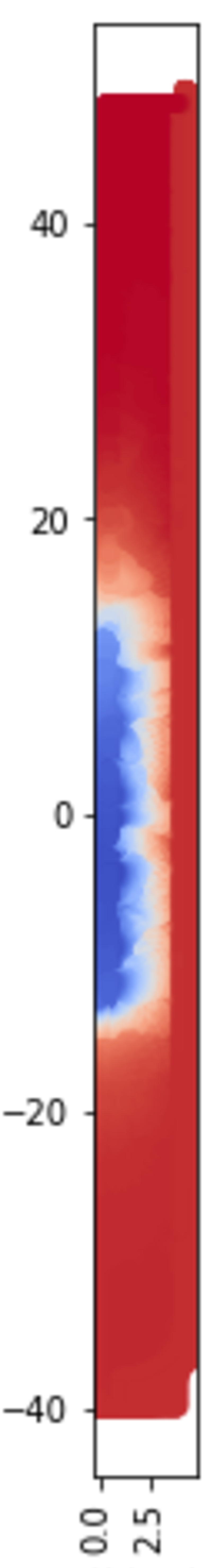
(c) $\sigma_{2}=0.0332$

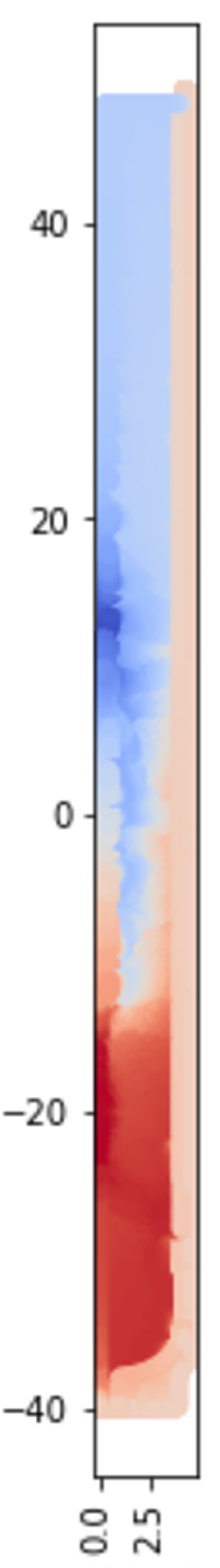
(d) $\sigma_{3}=0.0025$

Figure 12: Leading POD modes by energy contribution. The leading two modes capture approximately 99% of the energy content. Therefore, only five sensors corresponding to the leading five POD modes are required to reconstruct the heat advection near the heater region with high accuracy.

The leading two POD modes, which drive approximately 99% of the energy content, capture the heat advection from the heat source. Thus, only five sensors—corresponding to the first five POD modes—are required to reconstruct the flow with high accuracy. The cumulative energy content, along with a visualization of the first three POD modes, is given in Figure 12. These POD modes capture the interfaces between lower and higher temperatures as the advection flow progresses for different operating ranges.

Sensors placed at random locations fail to capture the underlying physics of the system. In 10(a), the introduction of bands of errors in the reconstruction occur where random sensors fail to accurately capture the transitions of temperature between hot and cold at a given gridpoint. Therefore, increasing the number of sensors selected does not significantly improve the reconstruction of the flow field. An ensemble of sensors placed at random locations produces large relative reconstruction errors that average approximately 35 as the number of sensors ($r$) is increased from 5 to 30, as seen in Figure 13. Random placement of sensors increases the reconstruction error by ten orders of magnitude. The random placement strategy alludes to data-agnostic sensor placement at best-guess locations for reconstructing temperature fields. The sensor placement algorithm was implemented in INL’s in-house Risk Analysis Virtual Environment (RAVEN) [60] framework.

\begin{overpic}[scale={.4},percent]{Figures/TWiSTrandom.png} \put(70.0,2.0){$(r)$} \end{overpic}

Figure 13: Error study. Proximity between the unconstrained and constrained QR selected sensors leads to orders of magnitude lower reconstruction error ($\epsilon\sim\mathcal{O}(10^{-1})$) compared to random placements. QR selected sensors accuracy increases with an increase in the number of selected sensors while random placements produce larger (approximately 35) relative reconstruction errors.

Unconstrained optimization favors locating sensors close to the heat source, due to the richer dynamics that exist there. Imposing sensor constraints within QR results in a near-optimal placement outside this region, as well as negligible loss of reconstruction performance. Moreover, the error decreases with more optimized sensors (unconstrained or constrained); however, random placements still suffer from high error even with additional sensors. Therefore, placing or adding sensors without optimizing them in regard to the underlying flow or deployment constraints can introduce large errors in the corresponding digital twins—and may even cause sensor damage. Incorporating such considerations prior to setting up a physical experiment enables precise uncertainty quantification and helps validate the predictions of a digital twin.

5 Discussion and Outlook

The reconstruction of reactor core flow fields using a limited budget of sensors has emerged as a critical enabler for digital twinning of nuclear assets. However, the challenge of achieving optimal sensing in high-dimensional real-world systems extends beyond the nuclear industry and encompasses diverse fields such as biology, physics, aviation, and automotive industries. Sensor placement in engineering systems is subject to various constraints, making the selection and optimal placement of sensors while considering these constraints a crucial aspect of algorithm development. In this study, we have developed strategies for placing sensors to satisfy constraints related to sensor proximity, regional limitations on sensor quantity, and design or user prescribed locations. Through these strategies, we have demonstrated the effectiveness of adaptive sensor placement in satisfying constraints while maintaining optimality and accuracy of the reconstructed responses of interest. Moreover, we showcase the scalability and broad applicability of the algorithms on a variety of applications and constraints.

Nevertheless, more complex constraints may arise in nuclear, fluid, or aerospace applications in which the capability to achieve flow reconstruction based on sparse measurements is indispensable. For instance, in each reactor region the maximum number of allowable sensors is usually design-specific and cannot be exceeded. Moreover, an emerging practice during nuclear fuels tests is the use of distributed sensors (e.g., fiber-optic sensors or multipoint thermocouples). A fiber bragg grating (FBG) is an example where the refraction index changes along the sensor length and provides distributed measurements. Designing fiber optic sensors—which act as line sensors with different measurements at each point on the line—is a novel challenge, as line sensors can be topologically shaped along various structures in engineering systems. Optimizing such topologies is another future direction for adaptive sensor placement. Fiber optic bundles are used for recreating high-quality images in both nuclear engineering and neuroscience. Optimizing the locations for these bundles so as to capture the best quality images is another interesting research direction for sparse sensing.

Furthermore, it might be very costly to place sensors in certain areas of the reactor, due to the need for specially designed sensors capable of withstanding harsh working conditions. Other areas may entail spatial constraints. Thus, multi-objective optimization based on optimizing both the cost and spatial locations of sensors is an interesting problem. Time-dependent dynamics and the study of transients is invaluable in the nuclear field. Sensor placement based on time-dependent data from OPTI-TWIST and the use of dynamic mode decomposition or a nonlinear embedding such as autoencoders is an interesting future direction for the developed sensor placement algorithm. In addition to the reconstruction of steady-state figures of merit, this research will attempt to progress towards addressing transients caused by power transients in test reactors such as TREAT. The ultimate goal is to extend the algorithms to inform users the optimal locations and timesteps to collect spatiotemporal sparse measurements to reconstruct core flow profiles during transients. This should naturally evolve to the capability of performing sensor optimal placement for multi-class classification, where the algorithm must select the sensor network capable of predicting which accident scenario is more likely to occur faster than real time. Examples of such accident scenarios include Loss of Coolant Accident (LOCA), Reactor Initiated Accidents (RIA), loss of power, etc. These scenarios can be easily realized in a non-destructive fashion within the TWIST prototype by opening a valve, or suddenly shutting the heater power off. Once successful, this work holds the potential to identify sensor maps capable of detecting off-normal conditions, anomalies, and injected signals, enhancing resilience and security of the physical twin against cyber-attacks.

Author Contribution

\begin{overpic}[scale={.39},percent]{Figures/AuthorContributionFinal.png} \end{overpic}

References

- [1] BR Upadhyaya, SRP Perillo, X Xu and F Li “Advanced control design, optimal sensor placement, and technology demonstration for small and medium nuclear power reactors” In International Conference on Nuclear Engineering 43550, 2009, pp. 763–773
- [2] M Grieves “Digital Twin: Manufacturing Excellence through Virtual Factory Replication-A Whitepaper by Dr. Michael Grieves” In White Pap, 2015, pp. 1–7
- [3] Michael Grieves and John Vickers “Digital twin: Mitigating unpredictable, undesirable emergent behavior in complex systems” In Transdisciplinary perspectives on complex systems Springer, 2017, pp. 85–113
- [4] Edward Glaessgen and David Stargel “The digital twin paradigm for future NASA and US Air Force vehicles” In 53rd AIAA/ASME/ASCE/AHS/ASC structures, structural dynamics and materials conference 20th AIAA/ASME/AHS adaptive structures conference 14th AIAA, 2012, pp. 1818
- [5] M Shafto, M Conroy, R Doyle, E Glaessgen, C Kemp, J LeMoigne and L Wang “NASA technology roadmap: modeling, simulation, information technology & processing roadmap technology area 11” In 2019–04–13]. https://www. nasa. gov/pdf/501321main_ TA11–ID_rev4_NRCwTASR. pdf, 2010
- [6] Eric J Tuegel, Anthony R Ingraffea, Thomas G Eason and S Michael Spottswood “Reengineering aircraft structural life prediction using a digital twin” In International Journal of Aerospace Engineering 2011 Hindawi, 2011
- [7] Eric Tuegel “The airframe digital twin: some challenges to realization” In 53rd AIAA/ASME/ASCE/AHS/ASC structures, structural dynamics and materials conference 20th AIAA/ASME/AHS adaptive structures conference 14th AIAA, 2012, pp. 1812
- [8] Houde Song, Meiqi Song and Xiaojing Liu “Online autonomous calibration of digital twins using machine learning with application to nuclear power plants” In Applied Energy 326 Elsevier, 2022, pp. 119995
- [9] Linyu Lin, Han Bao and Nam Dinh “Uncertainty quantification and software risk analysis for digital twins in the nearly autonomous management and control systems: A review” In Annals of Nuclear Energy 160 Elsevier, 2021, pp. 108362
- [10] Adil Rasheed, Omer San and Trond Kvamsdal “Digital twin: Values, challenges and enablers from a modeling perspective” In Ieee Access 8 IEEE, 2020, pp. 21980–22012
- [11] Dirk Hartmann, Matthias Herz and Utz Wever “Model order reduction a key technology for digital twins” In Reduced-order modeling (ROM) for simulation and optimization Springer, 2018, pp. 167–179
- [12] Lawrence Sirovich “Turbulence and the dynamics of coherent structures. I. Coherent structures” In Quarterly of applied mathematics 45.3, 1987, pp. 561–571
- [13] Karen Willcox and Jaime Peraire “Balanced model reduction via the proper orthogonal decomposition” In AIAA journal 40.11, 2002, pp. 2323–2330
- [14] Bernd R Noack, Konstantin Afanasiev, MAREK MORZYŃSKI, Gilead Tadmor and Frank Thiele “A hierarchy of low-dimensional models for the transient and post-transient cylinder wake” In Journal of Fluid Mechanics 497 Cambridge University Press, 2003, pp. 335–363
- [15] Jean-Christophe Loiseau, Bernd R Noack and Steven L Brunton “Sparse reduced-order modelling: sensor-based dynamics to full-state estimation” In Journal of Fluid Mechanics 844 Cambridge University Press, 2018, pp. 459–490
- [16] Clarence W Rowley “Model reduction for fluids, using balanced proper orthogonal decomposition” In International Journal of Bifurcation and Chaos 15.03 World Scientific, 2005, pp. 997–1013
- [17] Mohammad Abdo, Rabab Elzohery and Jeremy A Roberts “Modeling isotopic evolution with surrogates based on dynamic mode decomposition” In Annals of Nuclear Energy 129 Elsevier, 2019, pp. 280–288
- [18] R Elzohery, M Abdo and J Roberts “Comparison between gaussian processes and dmd surrogates for isotopic composition prediction” In Transactions of the American Nuclear Society 118, 2018, pp. 459–462
- [19] Mohammad Abdo, Rabab Elzohery and Jeremy A Roberts “Analysis of the LRA Reactor Benchmark Using Dynamic Mode Decomposition” In Trans. Am. Nucl. Soc 119, 2018, pp. 683
- [20] Christian Franzke, Andrew J Majda and Eric Vanden-Eijnden “Low-order stochastic mode reduction for a realistic barotropic model climate” In Journal of the atmospheric sciences 62.6 American Meteorological Society, 2005, pp. 1722–1745
- [21] DT Crommelin and AJ Majda “Strategies for model reduction: Comparing different optimal bases” In Journal of the Atmospheric Sciences 61.17, 2004, pp. 2206–2217
- [22] Tilmann Wittig, Rolf Schuhmann and Thomas Weiland “Model order reduction for large systems in computational electromagnetics” In Linear algebra and its applications 415.2-3 Elsevier, 2006, pp. 499–530
- [23] S Koziel and S Ogurtsov “Model management for cost-efficient surrogate-based optimisation of antennas using variable-fidelity electromagnetic simulations” In IET Microwaves, Antennas & Propagation 6.15 IET, 2012, pp. 1643–1650
- [24] Serhat Yeşilyurt and Anthony T. Patera “Surrogates for numerical simulations; optimization of eddy-promoter heat exchangers” In Computer methods in applied mechanics and engineering 121.1-4 Elsevier, 1995, pp. 231–257
- [25] HM Park and DH Cho “The use of the Karhunen-Loeve decomposition for the modeling of distributed parameter systems” In Chemical Engineering Science 51.1 Elsevier, 1996, pp. 81–98
- [26] Richard Everson and Lawrence Sirovich “Karhunen–Loeve procedure for gappy data” In JOSA A 12.8 Optica Publishing Group, 1995, pp. 1657–1664
- [27] Bruce Moore “Principal component analysis in linear systems: Controllability, observability, and model reduction” In IEEE transactions on automatic control 26.1 IEEE, 1981, pp. 17–32
- [28] Jer-Nan Juang and Richard S Pappa “An eigensystem realization algorithm for modal parameter identification and model reduction” In Journal of guidance, control, and dynamics 8.5, 1985, pp. 620–627
- [29] Zhaojun Bai, Patrick M Dewilde and Roland W Freund “Reduced-order modeling” In Handbook of numerical analysis 13 Elsevier, 2005, pp. 825–895
- [30] Pankaj Wahi and Vivek Kumawat “Nonlinear stability analysis of a reduced order model of nuclear reactors: A parametric study relevant to the advanced heavy water reactor” In Nuclear engineering and design 241.1 Elsevier, 2011, pp. 134–143
- [31] Dongli Huang, Hany Abdel-Khalik, Cristian Rabiti and Frederick Gleicher “Dimensionality reducibility for multi-physics reduced order modeling” In Annals of Nuclear Energy 110 Elsevier, 2017, pp. 526–540
- [32] Andreas Krause, Ajit Singh and Carlos Guestrin “Near-optimal sensor placements in Gaussian processes: Theory, efficient algorithms and empirical studies.” In Journal of Machine Learning Research 9.2, 2008
- [33] Siddharth Joshi and Stephen Boyd “Sensor selection via convex optimization” In IEEE Transactions on Signal Processing 57.2 IEEE, 2008, pp. 451–462
- [34] Tyler H Summers, Fabrizio L Cortesi and John Lygeros “On submodularity and controllability in complex dynamical networks” In IEEE Transactions on Control of Network Systems 3.1 IEEE, 2015, pp. 91–101
- [35] Bingni W Brunton, Steven L Brunton, Joshua L Proctor and J Nathan Kutz “Sparse sensor placement optimization for classification” In SIAM Journal on Applied Mathematics 76.5 SIAM, 2016, pp. 2099–2122
- [36] Kevin K Chen and Clarence W Rowley “H2 optimal actuator and sensor placement in the linearised complex Ginzburg–Landau system” In Journal of Fluid Mechanics 681 Cambridge University Press, 2011, pp. 241–260
- [37] Krithika Manohar, J Nathan Kutz and Steven L Brunton “Optimal sensor and actuator selection using balanced model reduction” In IEEE Transactions on Automatic Control 67.4 IEEE, 2021, pp. 2108–2115
- [38] Fei Tao, He Zhang, Ang Liu and Andrew YC Nee “Digital twin in industry: State-of-the-art” In IEEE Transactions on industrial informatics 15.4 IEEE, 2018, pp. 2405–2415
- [39] Bernd R Noack, Marek Morzynski and Gilead Tadmor “Reduced-order modelling for flow control” Springer Science & Business Media, 2011
- [40] Christophe Varé and Patrick Morilhat “Digital twins, a new step for long term operation of nuclear power plants” In Engineering Assets and Public Infrastructures in the Age of Digitalization Springer, 2020, pp. 96–103
- [41] J-P Argaud, Bertrand Bouriquet, F De Caso, Helin Gong, Yvon Maday and Olga Mula “Sensor placement in nuclear reactors based on the generalized empirical interpolation method” In Journal of Computational Physics 363 Elsevier, 2018, pp. 354–370
- [42] Siyao Gu and Miltiadis Alamaniotis “Radiation Sensor Placement using Reinforcement Learning in Nuclear Security Applications” In 2022 13th International Conference on Information, Intelligence, Systems & Applications (IISA), 2022, pp. 1–6 IEEE
- [43] Belle R Upadhyaya and Fan Li “Optimal sensor placement strategy for anomaly detection and isolation” In 2011 Future of Instrumentation International Workshop (FIIW) Proceedings, 2011, pp. 95–98 IEEE
- [44] Mengnan Liu, Shuiliang Fang, Huiyue Dong and Cunzhi Xu “Review of digital twin about concepts, technologies, and industrial applications” In Journal of Manufacturing Systems 58 Elsevier, 2021, pp. 346–361
- [45] Hossein Darvishi, Domenico Ciuonzo, Eivind Roson Eide and Pierluigi Salvo Rossi “Sensor-fault detection, isolation and accommodation for digital twins via modular data-driven architecture” In IEEE Sensors Journal 21.4 IEEE, 2020, pp. 4827–4838
- [46] Ronald Aylmer Fisher “Design of experiments” In British Medical Journal 1.3923 BMJ Publishing Group, 1936, pp. 554
- [47] Kirstine Smith “On the standard deviations of adjusted and interpolated values of an observed polynomial function and its constants and the guidance they give towards a proper choice of the distribution of observations” In Biometrika 12.1/2 JSTOR, 1918, pp. 1–85
- [48] Ashis Sengupta “Generalized variance” In Encyclopedia of statistical sciences 3.1 John Wiley & Sons Inc New York, New York, USA, 2004
- [49] Michael Friendly, Georges Monette and John Fox “Elliptical insights: understanding statistical methods through elliptical geometry”, 2013
- [50] Maxime Barrault, Yvon Maday, Ngoc Cuong Nguyen and Anthony T Patera “An ‘empirical interpolation’method: application to efficient reduced-basis discretization of partial differential equations” In Comptes Rendus Mathematique 339.9 Elsevier, 2004, pp. 667–672
- [51] Saifon Chaturantabut and Danny C Sorensen “Nonlinear model reduction via discrete empirical interpolation” In SIAM Journal on Scientific Computing 32.5 SIAM, 2010, pp. 2737–2764
- [52] Zlatko Drmac and Serkan Gugercin “A new selection operator for the discrete empirical interpolation method—improved a priori error bound and extensions” In SIAM Journal on Scientific Computing 38.2 SIAM, 2016, pp. A631–A648
- [53] Krithika Manohar, Bingni W Brunton, J Nathan Kutz and Steven L Brunton “Data-driven sparse sensor placement for reconstruction: Demonstrating the benefits of exploiting known patterns” In IEEE Control Systems Magazine 38.3 IEEE, 2018, pp. 63–86
- [54] Krithika Manohar, Thomas Hogan, Jim Buttrick, Ashis G Banerjee, J Nathan Kutz and Steven L Brunton “Predicting shim gaps in aircraft assembly with machine learning and sparse sensing” In Journal of manufacturing systems 48 Elsevier, 2018, pp. 87–95
- [55] Peter Businger and Gene H Golub “Linear least squares solutions by Householder transformations” In Numerische Mathematik 7.3 Springer, 1965, pp. 269–276
- [56] Emily Clark, Steven L Brunton and J Nathan Kutz “Multi-fidelity sensor selection: Greedy algorithms to place cheap and expensive sensors with cost constraints” In IEEE Sensors Journal 21.1 IEEE, 2020, pp. 600–611
- [57] Ming Gu and Stanley C Eisenstat “Efficient algorithms for computing a strong rank-revealing QR factorization” In SIAM Journal on Scientific Computing 17.4 SIAM, 1996, pp. 848–869
- [58] Benjamin Peherstorfer, Zlatko Drmac and Serkan Gugercin “Stability of discrete empirical interpolation and gappy proper orthogonal decomposition with randomized and deterministic sampling points” In SIAM Journal on Scientific Computing 42.5 SIAM, 2020, pp. A2837–A2864
- [59] Siemens Digital Industries Software “Simcenter STAR-CCM+, version 2021.1”, Siemens 2021
- [60] Cristian Rabiti, Andrea Alfonsi, Diego Mandelli, Joshua J Cogliati, Congjian Wang, Paul W Talbot, Daniel P Malijovec, Robert A Kinoshita, Mohammad Gamal Abdo and Sonat Sen “RAVEN user manual”, 2021