Fast Approximation of Unbalanced Optimal Transport and Maximum Mean Discrepancies

Abstract

This contribution presents significant computational accelerations to prominent schemes, which enable the comparison of measures, even with varying masses. Concisely, we employ nonequispaced fast Fourier transform to accelerate the radial kernel convolution in unbalanced optimal transport approximation, building on the Sinkhorn algorithm. Accelerated schemes are presented as well for the maximum mean discrepancies involving kernels based on distances. By employing nonequispaced fast Fourier transform, our approaches significantly reduce the arithmetic operations to compute the distances from $\mathcal{O}(n^{2})$ to $\mathcal{O}(n\log n)$, which enables access to large and high-dimensional data sets. Furthermore, we show some robust relation between the Wasserstein distance and maximum mean discrepancies. Numerical experiments using synthetic data and real datasets demonstrate the computational acceleration and numerical precision.

Mathematics Subject Classifications: 90C08, 90C15, 60G07

Keywords: Sinkhorn divergence • unbalanced optimal transport • NFFT • entropy

1 Introduction

The question of comparing given probability measures is an enthralling problem. Many progressive and remarkable formulations have been presented to address the problem. Among popular domains like data science, the restriction to formulations that can only handle measures of equal weight (probability measures, for example), is very often cumbersome. Some formulations have been proposed to handle general measures. However, the numerical acceleration of such formulations is not addressed enough in the literature. This paper focuses on numerical acceleration of prominent formulations, which enable the comparison of two measures with possibly different masses. Additionally, we provide theoretical bounds and relations between the taxonomy of distances presented below.

Optimal transport (OT) in its standard formulation builds on efficient ways to rearrange mass between two given probability distributions. Such approaches commonly relate to the Wasserstein or Monge–Kantorovich distance. We refer to the monograph Villani [39] for an extensive discussion of the OT problem. A pivotal constraint of the standard OT problem formulation is that it demands the input measures to be normalized to unit mass – that is, to probability measures. This is an unfeasible presumption for some problems that need to handle arbitrary, though positive measures. Unbalanced optimal transport (UOT) has been established to deal with this drawback by allowing mass variation in the transportation problem (cf. Benamou [3]). This problem is stated as a generalization of the Kantorovich formulation (cf. Kantorovich [15]) by taking aberrations from the desired measures into account in addition.

On the other hand, the strong foundation of kernel theories lead to many mathematical and computational advancements. One popular instance of such advancements is the reproducing kernel Hilbert space (RKHS), which is predominantly considered as an efficient tool to generalize the linear statistical approaches to non-linear settings, cf. the kernel trick, e.g. By utilizing the distinct mathematical properties of RKHS, a distance measure is proposed in Gretton et al. [14], which is known as maximum mean discrepancy (MMD). Maximum mean discrepancies (MMDs) are kernel based distance measures between given unbalanced and/ or probability measures, based on embedding measures in a RKHS. We refer to Muandet et al. [23] for a textbook reference. Remarkably, these kernel based distances provide meaningful metrics for unbalanced measures as well.

Numerical computation and applications of UOT and MMD.

The technique of entropy regularization to solve the standard OT problem is an important milestone, which improves the scalability of traditional methods (cf. Cuturi [10]). The Sinkhorn algorithm utilizes the entropy regularized OT problem (cf. Sinkhorn [34]). The unbalanced OT (UOT) problems splendidly adopt the entropy regularization technique, which also improves the scalability.

Today’s data-driven world, which is dominated by rapidly growing machine learning (ML) techniques, utilizes the entropy regularized UOT algorithm for many applications. These include, among various others, domain adaptation (cf. Fatras et al. [11]), crowd counting (cf. Ma et al. [22]), bioinformatics (cf. Schiebinger et al. [32]), and natural language processing (cf. Wang et al. [41]).

MMD is considered as an important framework for many problems in machine learning and statistics. For instance intelligent fault diagnosis (cf. Li et al. [19]), two-sample testing (cf. Gretton et al. [14]), feature selection (cf. Song et al. [36]), density estimation (cf. Song et al. [35]) and kernel Bayes’ rule (cf. Fukumizu et al. [12]), which are applicable fields based on MMD. In the MMD framework, the choice of the kernel plays a vital role, and it depends on the nature of the problem. The forthcoming sections explicitly explain the efficient computational approach for prominent kernels.

Related works and contributions.

Considering unbalanced measures (that is, measures of possibly different total mass) requires establishing divergences to more general measures than probability measures. We build our formulations on Bregman divergences. This approach includes divergences as the popular Kullback–Leibler divergence, which captures deviations for probability measures only.

Many algorithms have been proposed, including the entropy regularization approach, to efficiently solve UOT problems. Chizat et al. [9] investigate some prominent numerical approaches. In the research work of Carlier et al. [6], a method for fast Sinkhorn iterations, that involve only Gaussian convolutions, is theoretically studied. The core idea of this approach is that each step (i.e., each iteration) can be solved on a regular grid (equispaced), which is relatively faster than the standard Sinkhorn iteration. However, this approach utilizes the equispaced convolution, which is often a setback among the wide range of applications (cf. Platte et al. [28], Potts et al. [31, Section 1]), and also it renders an expense of approximation. Additionally, we refer to von Lindheim and Steidl [40], where the authors emphasize that the increased computational complexity and memory requirements of regularized UOT problems need to be addressed further.

Despite significant statistical advantages, MMD problems suffer from a computational burden. Unlike OT and UOT problems, only few contributions are presented to surpass the computational burden of MMD problems. Those few contributions improve the computational process at the price of substandard approximation accuracy (cf. Zhao and Meng [42], Le et al. [18]). Furthermore, some recent approaches, with focus on Gaussian kernel implementation, utilize the low-rank Nyström method to mitigate the computational burdens (cf. Cherfaoui et al. [8], Chatalic et al. [7]).

One of the top ten algorithms of the 20^th century is the fast Fourier transform (FFT), which relies on equispaced data points. The technique of FFT has been generalized to access non-equispaced data points, which is known as non-equispaced fast Fourier transform (NFFT). In contrast to FFT, NFFT is an approximate algorithm, but it renders stable computation at the same number of arithmetic operations as FFT.

To overcome the computational challenges set by UOT and MMDs, we present fast computational methods using non-equispaced convolution, which is known as fast summation method based on NFFT. The fast summation method used in the algorithms proposed below utilizes the standard entropy regularized OT problem, cf. Lakshmanan et al. [17]. It captures the precise nature of standard numerical algorithms and comes with significant improvements in terms of time and memory. This method can also be utilized for multi-marginal OT, a generalization of standard OT (cf. Ba and Quellmalz [2]). To the best of our knowledge, NFFT fast summation method has not been considered either in UOT nor in an MMD setup. Thus, this paper focuses on accelerating the computation of entropy regularized UOT and MMDs by utilizing the NFFT based fast summation, and we also provide some robust inequalities which explain the robust relation between Wasserstein distance and MMD. For MMD implementations, we present inverse multiquadratic and energy kernels in addition to Gaussian and Laplace kernels, as there is a demand for these kernels in the literature.

Outline of the paper.

Section 2 discusses the necessary definitions and properties of the UOT and MMD problem. Additionally, it provides relations between Wasserstein distances and MMD. In Section 3, we reformulate our problem of interest in the discrete setting, and explicitly explain its computational background. Section 4 introduces the fast summation technique based on NFFT, which promotes fast matrix-vector operations. It presents the NFFT accelerated implementation of regularized UOT and MMDs, which promises fast and stable computation. Additionally, we explain the arithmetic operations of the corresponding problems. Section 5 substantiates the performances of our proposed approaches using synthetic as well as real data sets.

2 Preliminaries and taxonomy of Wasserstein distances

In this section, we provide necessary definitions and properties to facilitate the upcoming discussion. Moreover, we introduce robust relations between MMD and Wasserstein distance, and upper bounds for the unbalance optimal transport.

2.1 Bregman divergence

In various domains, the Bregman divergence (cf. Bregman [5]) is utilized as a generalized measure of difference of two different points (cf. Lu et al. [21], Nielsen [26]). Here, we consider the deviation with regard to a strictly convex function on the set of non-negative Radon measures $\mathcal{M}_{+}(\mathcal{X})$, where $\mathcal{X}\subset\mathbb{R}^{d}$.

Definition 2.1 (Bregman divergence).

For a $\mathbb{R}$-valued, convex function $\Phi\colon\mathcal{M}_{+}(\mathcal{X})\to\mathbb{R}$, the Bregman divergence is

$$\mathrm{D}(\nu\|\mu)\coloneqq\Phi(\nu)-F_{\mu}(\nu)-\Phi(\mu),$$

where

$$F_{\mu}(\nu)\coloneqq\lim_{h\downarrow 0}\frac{1}{h}\left(\Phi\bigl{(}h\,\nu+(1-h)\mu\bigr{)}-\Phi(\mu)\right)$$

is the directional derivative of the convex function $\Phi$ at $\mu$ in direction $\nu-\mu$.

In statistics, $F_{\mu}$ is also called von Mises derivative or the influence function of $\Phi$ at $\mu$. Note that the Bregman divergence exists (possibly with values $\pm\infty$), and it is non-negative (that is, $\mathrm{D}(\nu\|\mu)\geq 0$), as the function $\Phi$ is convex by assumption and $\Phi(\nu)\geq\Phi(\mu)+F_{\mu}(\nu)$ (cf. the illustration in Figure 1). Uniform convexity causes definiteness (that is, $\mathrm{D}(\nu\|\mu)=0$ if and only if $\nu=\mu$) and the Bregman divergence, in general, is not symmetric.

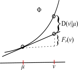
Figure 1: Bregman divergence between the measures $\mu$ and $\nu$

The Bregman divergence is notably defined here for general measures $\mu$ and $\nu$ in the domain of $\Phi$, including unbalanced measures (i.e., $\mu(\mathcal{X})\neq\nu(\mathcal{X})$); the Bregman divergence is particularly not restricted to probability measures.

Important examples for the Bregman divergence involve a non-negative reference measure $\mu$ and a convex function $\varphi$, and build on

$$\Phi(\nu)\coloneqq\int_{\mathcal{X}}\varphi\bigl{(}Z_{\nu}(\xi)\bigr{)}\,\mu(\mathrm{d}\xi),$$

where $Z_{\nu}$ is the Radon–Nikodým derivative of $\nu$ with respect to $\mu$; that is, $\nu(\mathrm{d}\xi)=Z_{\nu}(\xi)\,\mu(\mathrm{d}\xi)$. As $\varphi$ is convex and the measure $\mu$ positive, it follows from

$$\Phi\bigl{(}h\,\nu_{1}+(1-h)\nu_{0}\bigr{)} =\int_{\mathcal{X}}\varphi\left(h\,{\mathrm{d}\nu_{1}\over\mathrm{d}\mu}(\xi)+(1-h){\mathrm{d}\nu_{0}\over\mathrm{d}\mu}(\xi)\right)\,\mu(\mathrm{d}\xi)$$ (2.1)

$$\leq h\int_{\mathcal{X}}\varphi\left({\mathrm{d}\nu_{1}\over\mathrm{d}\mu}(\xi)\right)\mu(\mathrm{d}\xi)+(1-h)\int_{\mathcal{X}}\varphi\left({\mathrm{d}\nu_{0}\over\mathrm{d}\mu}(\xi)\right)\,\mu(\mathrm{d}\xi)$$ (2.2)

$$=h\,\Phi(\nu_{1})+(1-h)\,\Phi(\nu_{0})$$ (2.3)

that $\Phi$ is convex as well. For sufficiently smooth functions $\varphi$, it follows with the Taylor series expansion $\varphi(1+z)=\varphi(1)+\varphi^{\prime}(1)\,z+\mathcal{O}(z^{2})$ that

$$F_{\mu}(\nu) =\lim_{h\downarrow 0}{1\over h}\left(\int_{\mathcal{X}}\varphi\left(h\cdot{\mathrm{d}\nu\over\mathrm{d}\mu}(\xi)+1-h\right)\,\mu(\mathrm{d}\xi)-\int_{\mathcal{X}}\varphi(1)\,\mu(\mathrm{d}\xi)\right)\,$$ (2.4)

$$=\varphi^{\prime}(1)\cdot\int_{\mathcal{X}}\left({\mathrm{d}\nu\over\mathrm{d}\mu}(\xi)-1\right)\mu(\mathrm{d}\xi)$$ (2.5)

$$=\varphi^{\prime}(1)\,\nu(\mathcal{X})-\varphi^{\prime}(1)\,\mu(\mathcal{X}),$$ (2.6)

so that the Bregman divergence associated with $\Phi$ is

$$\mathrm{D}(\nu\|\mu) =\int_{\mathcal{X}}\varphi\Bigl{(}{\mathrm{d}\nu\over\mathrm{d}\mu}(\xi)\Bigr{)}\,\mu(\mathrm{d}\xi)+\varphi^{\prime}(1)\bigl{(}\mu(\mathcal{X})-\nu(\mathcal{X})\bigr{)}-\varphi(1)\,\mu(\mathcal{X}).$$ (2.7)

Using the aforementioned universalized formulation of Bregman divergence, the Bregman divergence corresponding to $\varphi(z)=z\log z$ is

$$\mathrm{D}_{\mathrm{KL}}(\nu\|\mu) =\int_{\mathcal{X}}\log\Bigl{(}{\mathrm{d}\nu\over\mathrm{d}\mu}\Bigr{)}\mathrm{d}\nu+\mu(\mathcal{X})-\nu(\mathcal{X}),$$ (2.8)

which generalizes the Kullback–Leibler divergence to general (unbalanced) measures $\nu$, provided that $\mu$ is a positive measure.

Remark 2.2.

The literature occasionally considers the slightly modified convex function

$$\varphi(z)=\begin{cases}z\log z-z+1&\text{if }z>0,\\ 1&\text{if }z=0\text{ and}\\ +\infty&\text{otherwise},\end{cases}$$ (2.9)

which results in the same generalized Kullback–Leibler divergence as stated in (2.8).

2.2 OT problem

The standard (i.e., balanced) OT problem is a linear optimization problem that reveals the minimal cost to transport masses from one probability measure to some other probability measure. The optimal cost is popularly known as the Wasserstein distance.

Definition 2.3 ($r$-Wasserstein distance).

The Wasserstein distance of order $r\geq 1$ of the probability measures $P$, ${\tilde{P}}\in\mathcal{P}(\mathcal{X})$ for a given cost or distance function $d\colon\mathcal{X}\times\mathcal{X}\to[0,\infty]$ is

$$\Bigg{(}\inf_{\pi\in\mathcal{P}(\mathcal{X}\times\mathcal{X})}\iint_{\mathcal{X}\times{\mathcal{X}}}d(x,\,{\tilde{x}})^{r}\,\pi(\mathrm{d}x,\mathrm{d}\tilde{x})\Bigg{)}^{1/r},$$ (2.10a)

where $$\pi P {\tilde{P}}$$ has marginal measures and , that is,

$$\tau_{1\#}\pi =P\text{ and}$$ (2.10b)

$$\tau_{2\#}\pi ={\tilde{P}},$$ (2.10c)

where $\tau_{1}(x,\tilde{x})\coloneqq x$ ($\tau_{2}(x,\tilde{x})\coloneqq\tilde{x}$, resp.) is the coordinate projection and $\tau_{1\#}\pi\coloneqq\pi\circ\tau_{1}^{-1}$ ($\tau_{2\#}\pi\coloneqq\pi\circ\tau_{2}^{-1}$, resp.) the pushforward measure.

More explicitly, the marginal constraints (2.10b)–(2.10c) are

$$\pi(A\times\mathcal{X}) =P(A)\text{ and}$$ (2.11)

$$\pi(\mathcal{X}\times B) ={\tilde{P}}(B),$$ (2.12)

where $A$ and $B\subset\mathcal{X}$ are measurable sets. We shall also write

$$\langle\pi|\,d^{r}\rangle\coloneqq\iint_{\mathcal{X}\times\mathcal{X}}d(\xi,\eta)^{r}\,\pi(\mathrm{d}\xi,\mathrm{d}\eta)$$

when averaging the function $d^{r}$ with respect to the measure $\pi$ as in (2.10a).

2.3 UOT problem

The marginal measures in (2.10b) and (2.10c) necessarily share the same mass, as $\tau_{1\#}\pi(\mathcal{X})=\pi(\mathcal{X}\times\mathcal{X})=\tau_{2\#}\pi(\mathcal{X})$. The core principle of the UOT problem is to relax the hard marginal constraints (2.10b) and (2.10c) with soft constraints to enable the mass variation. More concisely, the soft constraints are considered in the objective by involving the divergence between the marginals of $\pi$ from given measures $\mu$ and $\nu$.

In our research, we consider Bregman divergences as the soft constraints or marginal discrepancy function.

Definition 2.4 (Unbalanced optimal transport problem).

Let $\mu$, $\nu\in\mathcal{M}_{+}(\mathcal{X})$ and $d\colon\mathcal{X}\times\mathcal{X}\to[0,\infty)$. Let $\mathrm{D}(\cdot\|\cdot)$ be the Bregman divergence as in Definition 2.1. The generalized unbalanced transport cost is

$$\inf_{\pi\in\mathcal{M}_{+}(\mathcal{X}\times\mathcal{X})}\left\langle\pi|\,d^{r}\right\rangle+\eta_{1}\,\mathrm{D}(\tau_{1\#}\pi\|\,\mu)+\eta_{2}\,\mathrm{D}(\tau_{2\#}\pi\|\,\nu),$$ (2.13)

where $r\geq 1$. The parameter $\eta_{1}\geq 0$ ($\eta_{2}\geq 0$, resp.) is a regularization parameter, which emphasizes the importance assigned to the marginal measures $\mu$ ($\nu$, resp.).

The measure $\pi\in\mathcal{M}_{+}$ in (2.13) satisfies the relation $\tau_{1\#}\pi(\mathcal{X})=\tau_{2\#}\pi(\mathcal{X})$, although $\mu(\mathcal{X})\neq\nu(\mathcal{X})$ in general. The optimal measure in (2.13) thus constitutes a compromise between the total masses of $\mu$ and $\nu$. Note as well that the measure $\mu\otimes\nu$ is feasible in (2.13), with total measure $(\mu\otimes\nu)(\mathcal{X}\times\mathcal{X})=\mu(\mathcal{X})\cdot\nu(\mathcal{X})$.

Remark 2.5 (Marginal regularization parameters).

For parameters $\eta_{1}=\eta_{2}=0$ (or $\eta_{1}=\eta_{2}\searrow 0$, resp.), the explicit solution of problem (2.13) is $\pi=0$ ($\pi\searrow 0$, resp.). That is, no transportation takes place at all in this special case.

For $\eta_{1}\nearrow\infty$ and $\eta_{2}\nearrow\infty$, problem (2.13) appraises the marginals well. More precisely, for measures with equal mass, the solution $\pi$ tends to the solution of the standard optimal transport problem. In addition, the total mass of the optimal solution (2.13) increases from $\pi(\mathcal{X}\times\mathcal{X})=0$ to $\pi(\mathcal{X}\times\mathcal{X})=\mu(\mathcal{X})=\nu(\mathcal{X})$ (not $\mu(\mathcal{X})\cdot\nu(\mathcal{X})$). For measures with unequal mass, $\mu(\mathcal{X})\neq\nu(\mathcal{X})$, the transportation plan is the best plausible arrangement of the measures $\mu$ and $\nu$.

For a discussion on the minimizing measure and its existence we may refer to Liero et al. [20, Theorem 3.3].

2.4 Upper bounds for the unbalance optimal transport and relation to Wasserstein distance

Suppose the marginals $\tau_{1\#}\pi$ and $\tau_{2\#}\pi$ were known, then the Wasserstein problem in (2.13) is intrinsic. For this reason, we may consider the Wasserstein problem with normalized marginals to develop an upper bound for the unbalanced optimal transport problem.

Proposition 2.6.

Let $\pi$ be a bivariate probability measure, feasible for the Wasserstein problem with normalized marginals

$$P(\cdot)\coloneqq{\mu(\cdot)\over\mu(\mathcal{X})}\quad\text{ and }\quad{\tilde{P}}(\cdot)\coloneqq{\nu(\cdot)\over\nu(\mathcal{X})}.$$ (2.14)

Then

$$e^{-{\left\langle\pi|\,d^{r}\right\rangle\over\eta_{1}+\eta_{2}}}\cdot\mu(\mathcal{X})^{\eta_{1}\over\eta_{1}+\eta_{2}}\cdot\nu(\mathcal{X})^{\eta_{2}\over\eta_{1}+\eta_{2}}\cdot\pi$$ (2.15)

is an upper bound for the unbalanced optimal transport problem (2.13), and the constant in (2.15) is optimal among all measures of the form $c\cdot\pi$, where $c\geq 0$.

Specifically, the scaled product measure

$$e^{-{\left\langle\mu\otimes\nu|\,d^{r}\right\rangle\over(\eta_{1}+\eta_{2})\,\mu(\mathcal{X})\nu(\mathcal{X})}}\cdot{\mu\otimes\nu\over\mu(\mathcal{X})^{\eta_{2}\over\eta_{1}+\eta_{2}}\cdot\nu(\mathcal{X})^{\eta_{1}\over\eta_{1}+\eta_{2}}}$$

is an upper bound for (2.13).

Proof.

Let $\pi$ be any measure with marginals (2.14) and set $\pi_{c}\coloneqq c\cdot\pi$, where $c\geq 0$. It follows that

$$\tau_{1\#}\pi_{c}(\cdot)=c\cdot\pi(\cdot\times\mathcal{X})=c\cdot P(\cdot)=c\cdot{\mu(\cdot)\over\mu(\mathcal{X})}\text{ and}$$ (2.16)

$$\tau_{2\#}\pi_{c}(\cdot)=c\cdot\pi(\mathcal{X}\times\cdot)=c\cdot{\tilde{P}}(\cdot)=c\cdot{\nu(\cdot)\over\nu(\mathcal{X})},$$ (2.17)

so that the Radon–Nkodým derivatives are constant,

$${\mathrm{d}\tau_{1\#}\pi_{c}\over\mathrm{d}\mu}={c\,\over\mu(\mathcal{X})}\text{ and}$$ (2.18)

$${\mathrm{d}\tau_{2\#}\pi_{c}\over\mathrm{d}\nu}={c\over\,\nu(\mathcal{X})}.$$ (2.19)

It follows with (2.7) that the Kullback–Leibler divergences are

$$\mathrm{D}_{\mathrm{KL}}(\tau_{1\#}\pi_{c}\|\,\mu)={c\,\over\mu(\mathcal{X})}\log\Bigl{(}{c\,\over\mu(\mathcal{X})}\Bigr{)}\mu(\mathcal{X})+\mu(\mathcal{X})-c\text{ and}$$ (2.20)

$$\mathrm{D}_{\mathrm{KL}}(\tau_{2\#}\pi_{c}\|\,\nu)={c\,\over\nu(\mathcal{X})}\log\Bigl{(}{c\,\over\nu(\mathcal{X})}\Bigr{)}\nu(\mathcal{X})+\nu(\mathcal{X})-c.$$ (2.21)

Restricting the problem UOT to particular measures of the form $\pi_{c}=c\cdot\pi$, the objective of (2.13) reduces to

$$c\cdot\left\langle\pi|\,d^{r}\right\rangle +\eta_{1}\left({c\,\over\mu(\mathcal{X})}\log\Bigl{(}{c\,\over\mu(\mathcal{X})}\Bigr{)}\mu(\mathcal{X})+\mu(\mathcal{X})-c\right)$$ (2.22)

$$+\eta_{2}\left({c\,\over\nu(\mathcal{X})}\log\Bigl{(}{c\,\over\nu(\mathcal{X})}\Bigr{)}\nu(\mathcal{X})+\nu(\mathcal{X})-c\right),$$ (2.23)

where

$$\left\langle\pi|\,d^{r}\right\rangle\coloneqq\iint_{\mathcal{X}\times\mathcal{X}}d(x,\tilde{x})^{r}\,\pi(\mathrm{d}x,\mathrm{d}\tilde{x}).$$

Minimizing the objective (2.32) with respect to the constants $c>0$ reveals the best constant

$$c⃰=e^{-{\left\langle\pi|\,d^{r}\right\rangle\over\eta_{1}+\eta_{2}}}\cdot\mu(\mathcal{X})^{\eta_{1}\over\eta_{1}+\eta_{2}}\cdot\nu(\mathcal{X})^{\eta_{2}\over\eta_{1}+\eta_{2}}$$

and thus the first assertion.

The second assertion follows with $\pi\coloneqq{\mu\otimes\nu\over\mu(\mathcal{X})\cdot\nu(\mathcal{X})}$, as $\pi$ has marginals (2.14). ∎

Remark 2.7.

For increasing and equal regularization parameters, $\eta_{1}=\eta_{2}\to\infty$, the measure

$${\mu\otimes\nu\over\sqrt{\mu(\mathcal{X})\cdot\nu(\mathcal{X})}}$$

constitutes an upper bound. Further, for $\eta_{2}$ constant but $\eta_{1}\to\infty$, say, the measure in (2.15) approaches $\mu(\mathcal{X})\cdot\pi$: this measure has marginal $\mu$. Apparently, this is in line with the objective in (2.13), which forces the first marginal to approach $\mu$.

2.5 Entropy regularized UOT

The generic setup of UOT is computationally challenging. Thus, an entropy regularization approach was proposed, enabling computational efficiency with negligible compromise in accuracy.

Definition 2.8.

The entropy regularized, unbalanced optimal transport problem is

$${\text{UOT}}_{r;\eta;\lambda}(\mu,\nu)\coloneqq\inf_{\pi\in\mathcal{M}_{+}(\mathcal{X}\times\mathcal{X})}\left\langle\pi|\,d^{r}\right\rangle+{1\over\lambda}\,\mathrm{D}(\pi\|\,\mu\otimes\nu)+\eta_{1}\,\mathrm{D}(\tau_{1\#}\pi\|\,\mu)+\eta_{2}\,\mathrm{D}(\tau_{2\#}\pi\|\,\nu),$$ (2.24)

where $\pi$ is a non-negative, bivariate measure on $\mathcal{X}\times\mathcal{X}$; the parameter $r\geq 1$ is the order in the Wasserstein distance, $\lambda>0$ accounts for the entropy regularization and $\eta_{1}\geq 0$, $\eta_{2}\geq 0$ are the marginal regularization parameters.

Remark 2.9.

It is notable that the constants in (2.24) regularizing the marginals are $\eta_{1}$ and $\eta_{2}$ above, while the constant for the discrepancy of the entropy is $\nicefrac{{1}}{{\lambda}}$ (and not $\lambda$). We maintain the constant $1\over\lambda$ instead of $\lambda$ to stay consistent with preceding literature. To recover the initial Wasserstein problem (2.10a), it is essential that $\eta_{1}$ and $\eta_{2}$, as well as $\lambda$ are large or tend to $+\infty$.

As in Proposition 2.6 above, we can establish the following optimal compromise between the measures $\mu$ and $\nu$.

Proposition 2.10 (Optimal independent measure).

When restricted to measures $c\cdot\mu\otimes\nu$, $c\geq 0$, the measure

$$π⃰\coloneqq c⃰\cdot\mu\otimes\nu$$

with constant

$$c⃰\coloneqq e^{-{\left\langle\mu\otimes\nu|\,d^{r}\right\rangle\over\mu(\mathcal{X})\nu(\mathcal{X})(\eta_{1}+\eta_{2}+1/\lambda)}}\ \mu(\mathcal{X})^{-{\eta_{2}\over\eta_{1}+\eta_{2}+1/\lambda}}\ \nu(\mathcal{X})^{-{\eta_{1}\over\eta_{1}+\eta_{2}+1/\lambda}}$$ (2.25)

is optimal for the entropy regularized, unbalance optimal transport problem (2.24) with Kullback–Leibler divergences.

Proof.

Observe first that the marginal measures are

$$\tau_{1\#}\pi_{c}(\cdot)=\pi_{c}(\cdot\times\mathcal{X})=c\,\mu(\cdot)\nu(\mathcal{X})\text{ and}$$ (2.26)

$$\tau_{2\#}\pi_{c}(\cdot)=\pi_{c}(\mathcal{X}\times\cdot)=c\,\mu(\mathcal{X})\nu(\cdot),$$ (2.27)

so that the Radon–Nikodým derivatives are constant,

$${\mathrm{d}\pi_{c}\over\mathrm{d}\pi}=c,\qquad{\mathrm{d}\tau_{1\#}\pi_{c}\over\mathrm{d}\mu}=c\,\nu(\mathcal{X})\quad\text{ and }\quad{\mathrm{d}\tau_{2\#}\pi_{c}\over\mathrm{d}\nu}=c\,\mu(\mathcal{X}).$$ (2.28)

It follows with (2.7) that

$$\mathrm{D}_{\mathrm{KL}}(\pi_{c}\|\,\pi)=c\log(c)\cdot\mu(\mathcal{X})\nu(\mathcal{X})+\mu(\mathcal{X})\nu(\mathcal{X})-c\,\mu(\mathcal{X})\nu(\mathcal{X}),$$ (2.29)

and the Kullback–Leibler divergences of the marginals thus are

$$\mathrm{D}_{\mathrm{KL}}(\tau_{1\#}\pi_{c}\|\,\mu)=c\,\nu(\mathcal{X})\log\bigl{(}c\,\nu(\mathcal{X})\bigr{)}\mu(\mathcal{X})+\mu(\mathcal{X})-c\,\mu(\mathcal{X})\nu(\mathcal{X})\text{ and}$$ (2.30)

$$\mathrm{D}_{\mathrm{KL}}(\tau_{2\#}\pi_{c}\|\,\nu)=c\,\mu(\mathcal{X})\log\bigl{(}c\,\mu(\mathcal{X})\bigr{)}\nu(\mathcal{X})+\nu(\mathcal{X})-c\,\mu(\mathcal{X})\nu(\mathcal{X}).$$ (2.31)

Restricting the problem UOT to particular measures of the form $\pi_{c}=c\cdot\mu\otimes\nu$, the objective of (2.24) reduces to

$$c\cdot\left\langle\mu\otimes\nu|\,d\right\rangle +{1\over\lambda}\bigl{(}c\log(c)\cdot\mu(\mathcal{X})\nu(\mathcal{X})+c\,\mu(\mathcal{X})\nu(\mathcal{X})-\mu(\mathcal{X})\nu(\mathcal{X})\bigr{)}$$ (2.32)

$$+\eta_{1}\bigl{(}c\,\nu(\mathcal{X})\log\bigl{(}c\,\nu(\mathcal{X})\bigr{)}\mu(\mathcal{X})+c\,\mu(\mathcal{X})\nu(\mathcal{X})-\mu(\mathcal{X})\bigr{)}$$ (2.33)

$$+\eta_{2}\bigl{(}c\,\mu(\mathcal{X})\log\bigl{(}c\,\mu(\mathcal{X})\bigr{)}\nu(\mathcal{X})+c\,\mu(\mathcal{X})\nu(\mathcal{X})-\nu(\mathcal{X})\bigr{)}.$$ (2.34)

Minimizing the objective (2.32) with respect to the constants $c>0$ reveals the best measure explicitly as

$$π⃰\coloneqq c⃰\cdot\mu\otimes\nu,$$

where $c⃰$ as given in (2.25) is the best possible constant. ∎

The computation of optimal quantity $c⃰$ does not require any sophisticated optimization routine. This simple and efficient reformulation reveals the best upper bound of $\text{UOT}_{r;\eta;\lambda}(\mu,\nu)$, which is highly advantageous in many scenarios and can be used as a starting value in iterations in concrete implementations (see below).

2.6 Maximum mean discrepancies

Maximum mean discrepancy (MMD) embeds measures into a reproducing kernel Hilbert space (RKHS). This embedding gives rise to defining a distance on general, unbalance measures.

In what follows, we provide conditions so that the embedding is continuous with respect to the Wasserstein distance. As well, we demonstrate the fast computation of the new distance on unbalanced measures.

Definition 2.11 (Positive semi-definite).

The function $k\colon\mathcal{X}\times\mathcal{X}\to\mathbb{R}$ is a positive definite and symmetric kernel, if

$$\sum_{i=1}^{n}\sum_{j=1}^{n}c_{i}c_{j}k(x_{i},x_{j})\geq 0$$

for any scalars $(c_{1},\dots,c_{n})\in\mathbb{R}^{n}$ and $(x_{1},\dots,x_{n})\in\mathcal{X}^{n}$ and $n\in\mathbb{N}$.

Definition 2.12 (Reproducing kernel Hilbert space, cf. Berlinet and Thomas-Agnan [4]).

A Hilbert space $\mathcal{H}$ of functions from $\mathcal{X}\to\mathbb{R}$ (with inner product $\left\langle\cdot,\cdot\right\rangle_{\mathcal{H}}$) is a RKHS, if there is a positive semi-definite kernel $k\colon\mathcal{X}\times\mathcal{X}\to\mathbb{R}$, such that

1. $k_{x}(\cdot)\coloneqq k(\cdot,x)\in\mathcal{H}$ for all $x\in\mathcal{X}$,

2. $\left\langle k_{x},\varphi\right\rangle_{\mathcal{H}}=\varphi(x)$ for all $\varphi\in\mathcal{H}$ and $x\in\mathcal{X}$ (that is, the evaluation of the function $\varphi\in\mathcal{H}$ is a continuous, linear functional);

$k$ is called the reproducing kernel of $\mathcal{H}$ (cf. Aronszajn [1]).

Definition 2.13 (MMD).

Let $\mathcal{H}_{k}$ be an RKHS of $k\colon\mathcal{X}\times\mathcal{X}\to\mathbb{R}$ functions on $\mathcal{X}$. Then, the mean embedding is

$$\iota\colon\mathcal{M} \hookrightarrow\mathcal{H}_{k}$$ (2.35)

$$\mu \mapsto\mu_{k}(\cdot)\coloneqq\int_{\mathcal{X}}k(x,\cdot)\,\mu(\mathrm{d}x).$$ (2.36)

The RKHS distance between the mean embedding of given measures $\mu$ and $\nu$ is defined as

$$\text{MMD}_{k}(\mu,\nu)\coloneqq\|\mu_{k}-\nu_{k}\|_{\mathcal{H}_{k}}.$$

This RKHS distance is popularly known as MMD. Notably, it satisfies the axioms of a distance function. Further, given the elementary function $f(\cdot)=\sum_{j=1}^{n}w_{j}\,k(x_{j},\cdot)\in\mathcal{H}_{k}$, then $\iota(\mu)=f$ for the discrete measure $\mu(\cdot)=\sum_{j=1}^{n}w_{j}\,\delta_{x_{j}}$.

In other words, an RKHS-based interface between kernel methods and given distributions is offered by the mean embedding kernels. This distance is also occasionally referred as mean map kernel.

The critical relation to $\zeta$-metrics is given by the relation

$$\int_{\mathcal{X}}\varphi\,\mathrm{d}\mu=\int_{\mathcal{X}}\varphi(x)\,\mu(\mathrm{d}x)=\int_{\mathcal{X}}\left\langle\varphi(\cdot)|\,k(\cdot,x)\right\rangle\mu(\mathrm{d}x)=\left\langle\varphi(\cdot)\Big{|}\,\int_{\mathcal{X}}k(\cdot,x)\,\mu(\mathrm{d}x)\right\rangle=\left\langle\varphi|\,\mu_{k}\right\rangle,$$

so that

$$\int_{\mathcal{X}}\varphi\,\mathrm{d}\mu-\int_{\mathcal{X}}\varphi\,\mathrm{d}\nu=\left\langle\mu_{k}-\nu_{k}|\,\varphi\right\rangle\leq\|\mu_{k}-\nu_{k}\|_{\mathcal{H}_{k}}\,\|\varphi\|_{\mathcal{H}_{k}}.$$

or

$$\|\mu_{k}-\nu_{k}\|_{\mathcal{H}_{k}}=\sup_{\varphi\in B_{k}}\int_{\mathcal{X}}\varphi\,\mathrm{d}\mu-\int_{\mathcal{X}}\varphi\,\mathrm{d}\nu,$$ (2.37)

where the supremum is among all the functions $\varphi\in\mathcal{H}_{k}$ in the unit ball $B_{k}\subset\mathcal{H}_{k}$, $\|\varphi\|_{\mathcal{H}_{k}}\leq 1$.

Relation between MMD and Wasserstein

In what follows we relate the Wasserstein distance and MMD. To this end, consider first the measure $P=\delta_{x}$ ($Q=\delta_{y}$, resp.), the Dirac measure located at $x\in\mathcal{X}$ ($y\in\mathcal{X}$, resp.). Assuming that the kernel $k$ is bounded by $C$ ($k\leq C$), say, then

$$w_{p}(\delta_{x},\delta_{y})=d(x,y),$$ (2.38)

while

$$\|\delta_{x,k}-\delta_{y,k}\|^{2}_{\mathcal{H}_{k}}=\|k(\cdot,x)-k(\cdot,y)\|_{\mathcal{H}_{k}}^{2}=k(x,x)-2k(x,y)+k(y,y)\leq 2C.$$ (2.39)

It follows that the Wasserstein distance, in general, cannot be bounded by MMD on support sets $\mathcal{X}$ with unbounded diameter $\sup_{x,y\in\mathcal{X}}d(x,y)$. Note as well that $d(x,y)\coloneqq\|\delta_{x}-\delta_{y}\|_{\mathcal{H}_{k}}=\sqrt{k(x,x)-2k(x,y)+k(y,y)}$ defines a pseudo-metric on $\mathcal{X}$.

The following theorem provides conditions so that the embedding $\iota\colon\mathcal{M}\hookrightarrow\mathcal{H}_{k}$ is (Hölder-)continuous. It generalizes Vayer and Gribonval [38, Propostion 2] slightly to kernels, for which the unit ball in $\mathcal{H}_{k}$ is not necessarily uniformly Lipschitz, which includes the Laplacian kernel, e.g.

Proposition 2.14.

Let $P$ and $Q$ be probability measures. Suppose that

$$k(x,x)-2k(x,y)+k(y,y)\leq c^{2}\,d(x,y)^{2\alpha},\qquad x,y\in\mathcal{X},$$ (2.40)

for some $c>0$ and $\alpha\geq 1/2$. Then it holds that

$$\|P-Q\|_{\mathcal{H}_{k}}\leq c\,w_{\alpha}(P,Q)^{\alpha}.$$ (2.41)

Proof.

Let $\pi$ have marginals $P$ and $Q$. It follows with Jensen’s inequality that

$$|\operatorname{\mathds{E}}_{P}\varphi-\operatorname{\mathds{E}}_{Q}\varphi|^{2} =\left(\iint_{\mathcal{X}\times\mathcal{X}}\varphi(x)-\varphi(y)\,\pi(\mathrm{d}x,\mathrm{d}y)\right)^{2}$$ (2.42)

$$\leq\iint_{\mathcal{X}\times\mathcal{X}}\bigl{(}\varphi(x)-\varphi(y)\bigr{)}^{2}\,\pi(\mathrm{d}x,\mathrm{d}y).$$ (2.43)

Now assume that $\|\varphi\|_{\mathcal{H}_{k}}\leq 1$, then

$$|\varphi(x)-\varphi(y)|^{2} =|\left\langle\varphi(\cdot)|\,k(\cdot,x)\right\rangle-\left\langle\varphi|\,k(\cdot,y)\right\rangle|^{2}$$ (2.44)

$$=|\left\langle\varphi(\cdot)|\,k(\cdot,x)-k(\cdot,y)\right\rangle|^{2}$$ (2.45)

$$\leq\|\varphi\|_{\mathcal{H}_{k}}^{2}\cdot\|k(\cdot,x)-k(\cdot,y)\|_{\mathcal{H}_{k}}^{2}$$ (2.46)

$$\leq k(x,x)-2k(x,y)+k(y,y).$$ (2.47)

Together with (2.43) it follows that

$$|\operatorname{\mathds{E}}_{P}\varphi-\operatorname{\mathds{E}}_{Q}\varphi|^{2} \leq\iint_{\mathcal{X}\times\mathcal{X}}k(x,x)-2k(x,y)-k(y,y)\,\pi(\mathrm{d}x,\mathrm{d}y)$$ (2.48)

$$\leq\iint_{\mathcal{X}\times\mathcal{X}}c^{2}\,d(x,y)^{2\alpha}\,\pi(\mathrm{d}x,\mathrm{d}y),$$ (2.49)

where we have used the assumption (2.40) in (2.49). Maximizing the left-hand side with respect to all functions $\varphi\in\mathcal{H}_{k}$ with $\|\varphi\|_{\mathcal{H}_{k}}\leq 1$ using (2.37) and minimizing its right-hand side with respect to all measures $\pi$ with marginals $P$ and $Q$ reveals that

$$\|P_{k}-Q_{k}\|_{\mathcal{H}_{k}}^{2}\leq c^{2}\,w_{\alpha}(P,Q)^{2\alpha}.$$

Hence, the assertion. ∎

The kernels we consider below for fast summation techniques satisfy this general relation (2.40) with $\alpha=1$ and $\alpha=1/2$. Note that, for $\alpha=1/2$, the relation (2.41) reveals Hölder (and not Lipschitz) continuity of the embedding.

Prominent kernels.

In applications, the choice of the kernel function plays a vital role, and it depends on the problem of interest. The most prominent kernels used in MMDs are Gaussian (Gauss), inverse multi-quadratic (IMQ), Laplace (Lap) and energy (E) kernels. The following table (Tabel 1) provides these kernels, together with the constants in the preceding Proposition 2.14.

Kernel		Hölder exponent $\alpha$	Hölder constant
Gauss	$k^{\text{Gauss}}({x},\tilde{x})\coloneqq{e}^{\nicefrac{{-\|x-{\tilde{x}}\|^{2}}}{{\ell^{2}}}}$	$1$	$\nicefrac{{2}}{{\ell^{2}}}$
Laplace	$k^{\text{Lap}}({x},\tilde{x})\coloneqq{e}^{\nicefrac{{-\|x-{\tilde{x}}\|}}{{\ell}}}$	$1/2$	$\nicefrac{{2}}{{\ell}}$
Inverse multiquadratic	$k^{\text{IMQ}}(x,{\tilde{x}})\coloneqq\nicefrac{{1}}{{\sqrt{\|x-{\tilde{x}}\|^{2}+\mathrm{c}^{2}}}}$	$1$	$\nicefrac{{2}}{{c^{4}}}$
Energy	$k^{\text{e}}(x,{\tilde{x}})\coloneqq-\|x-{\tilde{x}}\|$	$1/2$	depends on $\mathcal{X}$

Table 1: Prominent kernels and their constant in relation to the Wasserstein distance, cf. (2.41)

The discrepancy obtained by using the energy kernel, $k^{\text{e}}$, is known as energy distance. The energy distance was originally proposed by Székely et al. [37], which is occasionally known as Harald Cramér’s distance. In general, the energy kernel is not positive definite although, for compact spaces $\mathcal{X}$, it is positive definite with a minor modification, cf. Neumayer and Steidl [25, Proposition 3.2]. Also, see Gräf [13, Corollary 2.15] for an explicit proof of conditional positivity of the energy kernel $k^{\text{e}}(\cdot,\cdot)$. The equivalence of energy distance and Cramér’s distance cannot be extended to higher dimensions because, unlike the energy distance, Cramér’s distance is not rotation invariant.

3 Distances in discrete framework

Computational aspects of the problems predominantly depend on discrete measures, which motivates us to investigate faster and stable computational methods. To this end, we reformulate the aforementioned problems in a discrete setting. More precisely, the unbalanced optimal transport problem must be stated in its dual version to accommodate the fast summation technique presented below. On the other hand, the maximum mean discrepancy formulation does not require any additional modifications.

The discrete measures considered in the following sections are $\mu=\sum_{i=1}^{n}\mu_{i}\,\delta_{x_{i}}$ and $\nu=\sum_{j=1}^{\tilde{n}}\nu_{j}\,\delta_{{\tilde{x}}_{j}}$.

3.1 Unbalanced optimal transport

To reformulate problem (2.24), we introduce the distance or cost matrix $d\in\mathbb{R}^{n\times{\tilde{n}}}$ with entries $d_{ij}\coloneqq d(x_{i},\tilde{x}_{j})$. With that, the discrete optimization problem (2.24) is

$$\text{UOT}_{r;\eta;\lambda}(\mu,\nu)=\inf_{\pi}\sum_{ij}d^{r}_{ij}\,\pi_{ij} +{1\over\lambda}\left(\sum_{ij}\pi_{ij}\log{\pi_{ij}\over\mu_{i}\nu_{j}}+\sum_{i,j}\mu_{i}\nu_{j}-\sum_{ij}\pi_{ij}\right)$$ (3.1)

$$+\eta_{1}\left(\sum_{i}\sum_{j}\pi_{ij}\log{\sum_{j^{\prime}}\pi_{ij^{\prime}}\over\mu_{i}}+\sum_{i}\mu_{i}-\sum_{i}\sum_{j}\pi_{ij}\right)$$ (3.2)

$$+\eta_{2}\left(\sum_{j}\sum_{i}\pi_{ij}\log{\sum_{i^{\prime}}\pi_{i^{\prime}j}\over\nu_{j}}+\sum_{i}\nu_{j}-\sum_{j}\sum_{i}\pi_{ij}\right).$$ (3.3)

Here, the matrix $\pi\in\mathbb{R}^{n\times{\tilde{n}}}$ with positive entries represents the transportation plan, and the parameters are as defined in Definition 2.8.

The duality reformulation gives rise to the accelerated algorithm of the UOT problem provided below. This explicit formulation justifies our advanced technique.

The following statement provides the dual formulation of the (primal) optimization problem (2.8), which is the foundation of our accelerated algorithm. The proof builds on the Fenchel-Rockafellar Theorem, and we may refer to Chizat et al. [9, Theorem 3.2].

Figure 2: Transportation (indicated by green lines) of measures (blue and red) with equal mass. The optimal transportation plan bypasses the outliers for smaller parameters $\eta$, and appraises for larger parameters $\eta$, cf. Remark 2.5.

Theorem 3.1 (Dualization of (2.24)).

For $\lambda>0$, $\eta_{1}>0$ and $\eta_{2}>0$, the dual function of entropy-regularized UOT (2.24) is

$$\mathcal{D}(\beta,\gamma)\coloneqq\max_{\beta\in\mathbb{R}^{n},\ \gamma\in\mathbb{R}^{\tilde{n}}} -\eta_{1}\sum_{i=1}^{n}{e}^{-\nicefrac{{\beta_{i}}}{{\eta_{1}}}}\mu_{i}-\eta_{2}\sum_{j=1}^{\tilde{n}}{e}^{-\nicefrac{{\gamma_{j}}}{{\eta_{2}}}}{\nu_{j}}+\,\eta_{1}\sum_{i=1}^{n}\mu_{i}+\,\eta_{2}\sum_{j=1}^{\tilde{n}}{\nu}_{j}$$ (3.4)

$$-\frac{1}{\lambda}\sum_{i=1}^{n}\sum_{j=1}^{\tilde{n}}\mu_{i}({e}^{\lambda\,\beta_{i}}\,{e}^{-\lambda\,d_{ij}^{r}}\,{e}^{\lambda\,\gamma_{j}}-1){\nu}_{j},$$ (3.5)

which results from a strictly concave, smooth, and unconstrained optimization problem. Strong duality is obtained for $\eta_{1}>0$ and $\eta_{2}>0$.

The duality result (3.4) gives rise to the well-known Sinkhorn’s algorithm. The unique maximizer $(β⃰,γ⃰)$ is described by the first-order optimality condition, and by alternating optimization (i.e., iterative procedure), we obtain a sequence $\gamma^{0},\beta^{1},\gamma^{1},\beta^{2},\dots$ as

$$\beta^{\Delta+1}=-{\eta_{1}\over 1+\eta_{1}\lambda}\log\big{(}k\,e^{\lambda\gamma^{\Delta}}\odot\,\nu\big{)}\quad\text{ and }\quad\gamma^{\Delta+1}=-{\eta_{2}\over 1+\eta_{2}\lambda}\log\big{(}k^{\top}\,e^{\lambda\beta^{\Delta}}\odot\mu\big{)},$$ (3.6)

where $\Delta\in\mathbb{N}$ is the iteration count, $\odot$ refers to the element wise dot product and $k\coloneqq e^{-\lambda\,d^{r}}$ (entrywise), and we may set $\gamma^{(0)}\coloneqq{\mathbf{0}}_{n}$. This is the basis for Sinkhorn’s iteration of regularized UOT. Sinkhorn’s theorem ensures that this alternating optimization routine converges to optimal solution (cf. Sinkhorn [34]).

Algorithm 1 summarizes the computational process, provides the optimal dual variable ($\beta^{Δ⃰}$ and $\gamma^{Δ⃰}$), and desired quantities can be computed using it. For instance, the proximate solution of the regularized UOT Problem (2.24) is

$$\pi^{Δ⃰}={e^{\lambda\beta^{Δ⃰}}}\,k\,{e^{\lambda\gamma^{Δ⃰}}}\odot(\mu\otimes\nu).$$

Remark 3.2 (Hyperparameter tuning and outliers).

In practice, we often fix $\eta_{1}=\eta_{2}\eqqcolon\eta$ to reduce the necessity of hyperparameter tuning.

From the consideration of Remark 2.5, we also deduce that, for finite values of $\eta$, problem (2.24) tends to ignore larger entries of the distance matrix $d$. That is, the solution of the problem does not involve outliers of the measures in the transportation. Figure 2 illustrates the impact of the parameters $\eta$, highlighting the transportation of outliers. Furthermore, if one prefers to strengthen the mass conservation of $\mu$ ($\nu$, resp.), it is achievable by increasing the marginal parameter $\eta_{1}$ ($\eta_{2}$, resp.).

Input: Distance $d_{ij}$ given in (4.1), positive vectors $\mu\in\mathbb{R}^{n}$, $\nu\in\mathbb{R}^{\tilde{n}}$, regularization parameter $\eta_{1}$, and $\eta_{2}$, entropy regularization parameter $\lambda>0$, $r\geq 1$, and starting value $\gamma=(\gamma_{1},\dots,\gamma_{\tilde{n}})$

Set

$$\,k_{ij}={e}^{-\lambda\,d_{ij}^{r}}\qquad i=1,\dots,n,\ j=1,\dots,{\tilde{n}}.$$ (3.7)

while stopping criteria do

       if $\Delta$ is odd then

            

$$\begin{split}\hskip 85.35826pt\beta_{i}^{\Delta}\leftarrow&-{\frac{\eta_{1}}{1+\eta_{1}\lambda}}\Big{(}\log\big{(}\sum_{j=1}^{\tilde{n}}k_{ij}\,{e}^{\lambda\,\gamma_{j}^{\Delta-1}}\,\nu_{j}\big{)}\Big{)},\quad i=1,\dots,n;\\ {\gamma}_{j}^{\Delta}\leftarrow&{\gamma}_{j}^{\Delta-1},\quad j=1,\dots,\tilde{n};\\[-9.04166pt] \end{split}$$ (3.8)

      else

            

$$\begin{split}\hskip 85.35826pt\gamma_{j}^{\Delta}\leftarrow&{-\frac{\eta_{2}}{1+\eta_{2}\lambda}}\Big{(}\log\big{(}\sum_{i=1}^{n}k_{ij}\,\mathrm{e}^{\lambda\,\beta_{i}^{\Delta-1}}\mu_{i}\big{)}\Big{)},\quad j=1,\dots,\tilde{n};\\ \beta_{i}^{\Delta}\leftarrow&\beta_{i}^{\Delta-1},\quad i=1,\dots,n;\\[-9.04166pt] \end{split}$$ (3.9)

      increment $\Delta\leftarrow\Delta+1$

Output: $\beta^{\Delta^{*}}$ and $\gamma^{\Delta^{*}}$

Algorithm 1 Sinkhorn algorithm to solve UOT (2.13)

Arithmetic complexity.

Even though the entropy regularization approach relaxes the computational burden, it still requires matrix-vector operation in (3.8) and (3.9) for each iteration, which are $\mathcal{O}(n^{2})$ arithmetic operations. The complete iteration routine of Algorithm 1 approximately requires

$$\mathcal{O}\big{(}\eta\lambda\,(\mu+\nu)\,n^{2}\log n\,\big{)}$$

arithmetic operations (cf. Pham et al. [27]) to achieve machine precision.

The exposition on fast summation techniques in Section 4 below takes advantage of the specific structure of the matrix $k=e^{-\lambda\,d^{r}}$ in (3.8) and (3.9), which is known as Gibbs kernel and/ or kernel matrix.

3.2 Computational aspects of MMDs

For discrete measures $\mu$ and $\nu$ as above, the numerical computation of $\text{MMD}^{2}_{k}(\mu,\nu)$ in terms of the corresponding kernel function $k$ is based on

$$\text{MMD}^{2}_{k}(\mu,\nu)=\sum_{i=1}^{n}\sum_{j=1}^{n}\mu_{i}\,\mu_{j}\,k(x_{i},x_{j})-2\sum_{i=1}^{n}\sum_{j=1}^{\tilde{n}}\mu_{i}\,\nu_{j}\,k(x_{i},\tilde{x}_{j})+\sum_{i=1}^{\tilde{n}}\sum_{j=1}^{\tilde{n}}\nu_{i}\,\nu_{j}\,k(\tilde{x}_{i},\tilde{x}_{j}).$$ (3.10)

The important observation here is that the individual terms in (3.10) constitute matrix vector multiplications, where the matrix has the same shape as in (3.6), cf. also Algorithm 1.

Arithmetic complexity.

In order to compute $\text{MMD}^{2}_{k}(\mu,\nu)$ or $\text{MMD}^{2}_{k}(P,{\tilde{P}})$, the standard implementation (3.10) requires $\mathcal{O}(n^{2}\,d)$ arithmetic operations, where $d$ is the dimension and $n\approx{\tilde{n}}$.

4 Fast summation method based on nonequispaced FFT

This section succinctly describes the nonequispaced Fourier transform (NFFT) based fast summation technique. In a nutshell, this technique allows reducing the computational burden of matrix-vector multiplications, which is $\mathcal{O}(n^{2})$ arithmetic operations. The forthcoming discussion explicitly provides the arithmetic operations of our fast algorithms, which are proposed to solve entropy regularized UOT and MMDs.

The standard kernel matrix-vector operation resembles the multiplication of the Toeplitz matrix with the vector. One can take advantage of this scenario to optimize $\mathcal{O}(n^{2})$ to $\mathcal{O}(n\log n)$ arithmetic operations, using a fast algorithm (cf. Plonka et al. [29, Theorem 3.31]). In other words, the fast algorithm embeds the kernel matrix into a circulant matrix, which is a special case of the Toeplitz matrix, and it diagonalizes the matrix using the Fourier matrix. This approach leads to the computation advancement, which is achieved using standard FFT (cf. Plonka et al. [29, pp. 141–142]).

Despite the benchmark computational advancement, standard FFT deteriorates by the restriction to equispaced points ($x_{i}$, $\tilde{x}_{j}$). Thus, the NFFT fast algorithm is introduced, which follows the similar approach for arbitrary points, see Plonka et al. [29, Chapter 7]. We refer to Keiner et al. [16] for a detailed interpretation of affiliated software.

4.1 NFFT fast summation

The fast summation method, which is based on NFFT, makes use of the radial distance

$$d(x,{\tilde{x}}):=\|x-{\tilde{x}}\|,$$

which builds on the difference of $x$ and ${\tilde{x}}$; the distance matrix $d\in\mathbb{R}^{n\times\tilde{n}}$ is

$$d(x_{i},\tilde{x}_{j})\coloneqq\|x_{i}-\tilde{x}_{j}\|,\quad i=1,\dots,n,\quad j=1,\dots,{\tilde{n}}.$$ (4.1)

Remark 4.1 (Radial cost functions).

The fast summation technique presented below crucially builds on radial cost functions. The cost functions contemplated here are increasing functions of the genuine distance $d$, for example $d^{r}$. This type of cost functions is commonly referred to as radial transport cost.

The core concept of fast summation is to efficiently approximate the radial kernels, i.e.,

$$\mathcal{K}^{\text{Gauss}}(y)\coloneqq e^{-\nicefrac{{\|y\|^{2}}}{{\ell^{2}}}},\quad\mathcal{K}^{\text{IMQ}}(y)\coloneqq\nicefrac{{1}}{{\sqrt{\|y\|^{2}+\mathrm{c}^{2}}}},\quad\mathcal{K}^{\text{Lap}}(y)\coloneqq e^{-\nicefrac{{\|y\|}}{{\ell}}},\quad\mathcal{K}(y)^{\text{abs}}\coloneqq\|y\|,$$

where $y\coloneqq x-\tilde{x}$ ($\ell>0$ and $c>0$).

Figure 3: Gaussian (blue), inverse multiquadric (red), Laplace (green) and energy or absolute value (violet).

The fast summation approach, which performs matrix-vector operation, computes sums of the form

$$s({x}_{i})\coloneqq\sum_{j=1}^{{\tilde{n}}}\mathcal{K}(x_{i}-\tilde{x}_{j})\,\tilde{\alpha}_{j},\quad i=1,\dots,n,$$ (4.2)

where coefficients $\tilde{\alpha}_{j}\in\mathbb{C}$ for all $j$.

4.2 Approximation aspects of kernel approximation

The central idea of NFFT is to efficiently approximate $\mathcal{K}(y)$ by an $h$-periodic trigonometric polynomial $\mathcal{K}_{RK}(y)$. To illustrate, we approximate a univariate kernel using a trigonometric polynomial in one dimension via

$$\mathcal{K}(y)\approx\mathcal{K}_{RK}(y)\coloneqq\sum_{\mathrm{k}\in\mathcal{I}_{N}}b_{\mathrm{k}}\,e^{2\pi\mathrm{i}\mathrm{k}y/h},\quad\mathcal{I}_{N}\coloneqq\Big{\{}-\frac{N}{2},-\frac{N}{2}+1,\dots,-1,0,\dots,\frac{N}{2}-1\Big{\}},$$ (4.3)

where $b_{\mathrm{k}}\in\mathbb{C}$ are appropriate Fourier coefficients, $y=x-\tilde{x}$ and bandwidth $N\in 2\mathbb{N}$. In order to efficiently compute the matrix-vector operations (4.2), which is a bottleneck of UOT and MMDs, the fast summation based on NFFT approximates $\mathcal{K}$ by the trigonometric polynomial $\mathcal{K}_{RK}$ with machine precision.

Note, that the desired kernels are non-periodic functions. Hence, an approximation using a trigonometric polynomial is not forthright. In order to obtain an $h$-periodic smooth kernel function $\tilde{\mathcal{K}}(y)$, we regularize ${\mathcal{K}}(y)$ as follows. If the argument $y$ satisfies $\|y\|\leq L$, we choose $h\geq 2L$. For a good approximation, we embed $\mathcal{K}(y)$ into a smooth periodic function by

$$\tilde{\mathcal{K}}(y)\coloneqq\begin{cases}\mathcal{K}(y)&\text{if }y\in[-L,L],\\ \mathcal{K}_{\mathrm{B}}(\|y\|)&\text{if }y\in(L,L+h),\end{cases}$$

where $\mathcal{K}_{\mathrm{B}}$ is a univariate polynomial, which matches the derivatives of $\mathcal{K}(y)$ up to a certain degree. This makes its periodic continuation $\tilde{\mathcal{K}}(y)$ smooth. We refer to Plonka et al. [29, Chapter 7.5] for more mathematical details.

In the one dimensional (univariate) case, we obtain the fast computation of distance matrix-vector operation by replacing the kernel $\mathcal{K}$ in (4.2) with corresponding Fourier representation (4.3). More specifically,

$$s(x_{i})\approx \sum_{j=1}^{\tilde{n}}\tilde{\alpha}_{j}\sum_{\mathrm{k}\in\mathcal{I}_{N}}b_{\mathrm{k}}e^{2\pi\mathrm{i}\mathrm{k}(\bar{x}_{i}-\bar{\tilde{x}}_{j})}$$ (4.4)

$$= \sum_{\mathrm{k}\in\mathcal{I}_{N}}b_{\mathrm{k}}\left(\sum_{j=1}^{\tilde{n}}\tilde{\alpha}_{j}e^{-2\pi\mathrm{i}\mathrm{k}\bar{\tilde{x}}_{j}}\right)e^{2\pi\mathrm{i}\mathrm{k}\bar{x}_{i}},\quad i=1,\dots,n,$$ (4.5)

with scaled nodes $\bar{x}_{i}\coloneqq h^{-1}x_{i}\in\mathbb{T}^{d}$, $\bar{\tilde{x}}_{j}\coloneqq h^{-1}\tilde{x}_{j}\in\mathbb{T}^{d}.$ Here, the torus $\mathbb{T}$ is

$$\mathbb{T}=\mathbb{R}\mod\mathbb{Z}\simeq\Big{[}-\frac{1}{2},\frac{1}{2}\Big{)}.$$

In the aforementioned setup, the inner sum in (4.5) is computed by the NFFT in $\mathcal{O}(N\log N+\tilde{n})$ arithmetical operations and the outer sum with $\mathcal{O}(N\log N+n)$. This ansatz generalizes to the multivariate setting.

Remark 4.2 (Arithmetic complexity).

Evaluating (4.2) with Gaussian kernel $\mathcal{K}^{\text{Gauss}}$ requires $\mathcal{O}(n+{\tilde{n}})$ arithmetic operations; with Laplacian $\mathcal{K}^{\text{Lap}}$, inverse multiquadratic $\mathcal{K}^{\text{IMQ}}$ and absolute value $\mathcal{K}^{\text{e}}$ kernel, $\mathcal{O}(n\log n+{\tilde{n}}\log{\tilde{n}})$ arithmetic operations are required. We refer to Plonka et al. [29, Chapter 7.5] for a comprehensive discussion.

Remark 4.3 (Curse of dimensionality).

Despite the robustness of NFFT, the evaluation is expensive for larger dimensions ($\mathcal{X}=\mathbb{R}^{d}$, where $d\geq 4$). In simple terms, NFFT suffers from curse of dimensionality. More specifically, for larger dimension, the grid $\mathcal{I}_{N}$ (cf. (4.3)) grows exponentially, which makes the evaluation expensive. To mitigate this burden, several research works have been presented in literature, which are predominantly based on mutual information score and Analysis of Variance (ANOVA) (cf. Nestler et al. [24], Potts and Schmischke [30]).

Remark 4.4 (Stabilization).

The accuracy of the regularized UOT problem depends on the regularization parameter $\lambda$. For larger $\lambda$, the kernel function concentrates on a smaller interval. In this case, involving a scaling factor $h$ as above, truncates the sum (4.2) to reach the desirable $\lambda$.

Input: support nodes $x_{i}$ and $\tilde{x}_{j}$, positive vectors $\mu\in\mathbb{R}^{n}$, $\nu\in\mathbb{R}^{\tilde{n}}$, entropy regularization parameter $\lambda>0$, $r\geq 1$, and starting value $\gamma=(\gamma_{1},\dots,\gamma_{\tilde{n}})$

while stopping criteria do

       Set

$${\gamma}^{(0)}={\mathbf{0}}_{\tilde{n}}.$$ (4.6)

      if $\Delta$ is odd then

            compute

$$t_{i}^{\Delta-1}\leftarrow\sum_{j=1}^{\tilde{n}}e^{-\lambda\|x_{i}-\tilde{x}_{j}\|^{r}}\cdot\nu_{j}e^{\lambda\,\gamma_{j}^{\Delta-1}},\quad i=1,\dots,n,$$

by employing the fast summation (4.4) and set

$$\begin{split}\beta_{i}^{\Delta}\leftarrow&{-\frac{\eta_{1}}{1+\eta_{1}\lambda}}\Big{(}\log t_{i}^{\Delta-1}\Big{)},\quad i=1,\dots,n;\\ \gamma_{j}^{\Delta}\leftarrow&\gamma_{j}^{\Delta-1},\quad j=1,\dots,\tilde{n}.\\[-6.02777pt] \end{split}$$ (4.7)

      else

            compute

$$\tilde{t}_{j}^{\Delta-1}\leftarrow\sum_{i=1}^{n}{e}^{-\lambda\|x_{i}-\tilde{x}_{j}\|^{r}}\cdot\mu_{i}{e}^{\lambda\,\beta_{i}^{\Delta-1}},\quad j=1,\dots,\tilde{n},$$

by employing the fast summation (4.4) and set

$$\begin{split}\gamma_{j}^{\Delta}\leftarrow&{-\frac{\eta_{2}}{1+\eta_{2}\lambda}}\Big{(}\log\tilde{t}_{j}^{\Delta-1}\Big{)},\quad j=1,\dots,\tilde{n};\\ \beta_{i}^{\Delta}\leftarrow&\beta_{i}^{\Delta-1},\quad i=1,\dots,n.\\[-6.02777pt] \end{split}$$ (4.8)

      increment $\Delta\leftarrow\Delta+1$

Result: $\beta^{\Delta^{*}}$ and $\gamma^{\Delta^{*}}$

Algorithm 2 NFFT-accelerated, Sinkhorn algorithm UOT

Arithmetic complexity of Algorithm 2.

For the sake of simplicity, we assume $n=\tilde{n}$. If $r=1$ (Laplacian kernel), Algorithm 2 requires

$$\mathcal{O}\big{(}\eta\lambda\,(\mu+{\nu})\,n\,(\log n)^{2}\,\big{)}$$

arithmetic operations to achieve machine accuracy. If $r=2$ (Gaussian Kernel), it requires

$$\mathcal{O}\big{(}\eta\lambda\,(\mu+{\nu})\,n\,(\log n)\,\big{)}$$

arithmetic operations (cf. Remark 4.2).

Arithmetic complexity of NFFT-accelerated MMD.

To compute MMD using Gaussian $\mathcal{K}^{\text{Gauss}}$, it requires

$$\mathcal{O}(n\,d)$$

arithmetic operations, and to compute MMD using Laplace $\mathcal{K}^{\text{Lap}}$, inverse multiquadric $\mathcal{K}^{\text{IMQ}}$ and absolute value $\mathcal{K}^{\text{abs}}$ kernels, it requires

$$\mathcal{O}(n\,\log n\,d)$$

arithmetic operations. Here, $d$ is the dimension.

5 Numerical exposition of the NFFT accelerated UOT and MMD

In this section, we demonstrate the numerical results for the approaches and methods considered in the preceding sections. The corresponding Julia implementations are available online. The implementation of NFFT techniques are based on the freely available repository ‘NFFT3.jl’. All experiments were performed on a standard desktop computer with Intel(R) Core(TM) i7-7700 CPU and 15.0 GB of RAM. Additionally, we emphasize that our proposed methods do not require expensive hardware or having access to supercomputers which is highly advantageous in terms of access to wide and low-threshold applications.

5.1 UOT acceleration

In this section, we illustrate the performance and accuracy of UOT NFFT Sinkhorn’s Algorithm 2 using synthetic and benchmark data.

5.1.1 Empirical measures

We demonstrate the efficiency (in terms of time and memory allocations) of our proposed Algorithm 2 using synthetic data.

Consider the measures

$$\mu={1\over n}\sum_{i=1}^{n}\mu_{i}\,\delta_{(U^{1}_{i},U^{2}_{i})}\quad\text{ and }\quad\nu={1\over{\tilde{n}}}\sum_{j=1}^{\tilde{n}}\nu_{j}\,\delta_{(\tilde{U}_{j}^{1},\tilde{U}_{j}^{2})}$$

on $\mathbb{R}\times\mathbb{R}$, where $U^{1}_{i}$, $U^{2}_{i}$, $\tilde{U}_{j}^{1}$, $\tilde{U}_{j}^{2}$, as well as the weights $\mu_{i}$ and $\nu_{j}$, are independent samples from the uniform distribution on $[0,1]$ ($i=1,\dots n$, $j=1,\dots,\tilde{n}$).

$n=\tilde{n}$:	$1000$		$10\,000$		$100\,000$		$1\,000\,000$
	Time	Memory	Time	Memory	Time	Memory	Time	Memory
	(Sec)	(MB)	(Sec)	(MB)	(Sec)	(MB)	(Sec)	(MB)
One dimension ($d=1$)
UOT Sinkhorn’s Alg.  1	$0.20$	$210.73$	$23.08$	$20\,655.10$	out of memory
UOT NFFT Sinkhorn’s Alg. 2	$0.09$	$12.64$	$0.43$	$150.28$	$4.47$	$1495.04$	$39.53$	$15\,022.08$
Two dimension ($d=2$)
UOT Sinkhorn’s Alg.  1	$0.63$	$256.51$	$25.60$	$25\,233.40$	out of memory
UOT NFFT Sinkhorn’s Alg. 2	$0.72$	$12.69$	$2.04$	$150.73$	$9.08$	$1507.32$	$77.24$	$15\,067.13$
Three dimension ($d=3$)
UOT Sinkhorn’s Alg. 1	$10.63$	$465.98$	$67.21$	$37\,324.46$	out of memory
UOT NFFT Sinkhorn’s Alg. 2	$31.32$	$18.32$	$100.54$	$191.13$	$202.17$	$1505.28$	$419.27$	$15\,114.24$

Table 2: Performance analysis of regularized UOT vs. NFFT accelerated–regularized UOT for varying dimensions; the accelerated algorithm manages problem sizes, which are out of reach for standard implementations Parameters: $r=2$, $\lambda=20$ and $\eta=1$; the best results are highlighted

Table 2 demonstrates computation times and memory allocations of UOT Sinkhorn’s Algorithm 1 and UOT NFFT Sinkhorn’s Algorithm 2. Our NFFT accelerated algorithm significantly outperforms the standard algorithm. Notably, our proposed algorithm easily reaches problem sizes, which are completely inaccessible for standard implementations.

5.1.2 Benchmark datasets

To unleash the exact ground truth of our proposed algorithm, we perform an accuracy analysis using benchmark datasets.

We employ the DOTmark dataset, which is explicitly designed to validate the performance and accuracy of new OT techniques and algorithms (cf. Schrieber et al. [33]). The DOTmark dataset consists of 10 subsets of gray scale images, ranging from $32\times 32$ to $512\times 512$ resolution.

Transformation of images to (unbalanced) vectors.

The grayscale image is given as a matrix, with each entry representing the intensity of a pixel in the range $[0,1]$ (black: 0, white: 1). The standard OT problem would – inappropriately – normalize the matrix. Our approach to UOT does not require normalizing the measure. Moreover, background pixel intensities are the $\ell_{1}$ distance between pixels $i$ and $j$ of the respective grids $(32\times 32,\dots$, and $512\times 512)$.

We compute the percent error,

$$\text{Residual}=\Bigg{(}\frac{\|\beta^{*}_{\text{NFFT}}-\beta^{*}\|}{\|\beta^{*}\|}+\frac{\|\gamma^{*}_{\text{NFFT}}-\gamma^{*}\|}{\|\gamma^{*}\|}\Bigg{)}\times 100,$$

where $\beta^{*}$ and $\gamma^{*}$ are optimal dual variable of UOT Sinkhorn’s Algorithm 1 and $\beta^{*}_{\text{NFFT}}$ and $\gamma^{*}_{\text{NFFT}}$ are optimal dual variable of UOT NFFT Sinkhorn’s Algorithm 2, to substantiate the accuracy of our proposed algorithm.

$n=\tilde{n}:$	$1024$	$4029$	$16\,384$
Dataset: DOTmark	Average residual
	$4.89\text{\times}{10}^{-12}$$\,\%$	$3.86\text{\times}{10}^{-12}$$\,\%$	$3.71\text{\times}{10}^{-12}$$\,\%$

Table 3: Accuracy analysis: NFFT accelerated–regularized UOT; Parameters $r=2$, $\lambda=20$ and $\eta=1$

Table 3 comprises the results of our accuracy analysis. From the results, it is evident that our proposed algorithm provides machine accuracy as promised. We skip the precise results for the sake of brevity. Although, we would like to emphasize that our proposed algorithm is capable of withstanding from smooth to rough nature of problems provided by DOTmark datasets.

5.2 MMDs accelerations

This section demonstrates the performance and accuracy of NFFT accelerated MMDs. We perform the experiments using the measures $\mu$ and $\nu$ as described in Section 5.1.1 above.

Kernels	Gaussian	Laplace	Inverse multi-quadratic	Energy
	Average residual
probability vectors	$2.42\text{\times}{10}^{-9}$$\,\%$	$1.10\text{\times}{10}^{-4}$$\,\%$	$6.03\text{\times}{10}^{-5}$$\,\%$	$5.30\text{\times}{10}^{-5}$$\,\%$
arbitrary (unbalanced) vectors	$1.31\text{\times}{10}^{-6}$$\,\%$	$2.04\text{\times}{10}^{-4}$$\,\%$	$2.84\text{\times}{10}^{-5}$$\,\%$	Nil

Table 4: Accuracy analysis: NFFT accelerated MMDs; Hyperparameters $\mathrm{c}=1$, $\ell=\frac{1}{2}$; dimension $d=2$; problem size ranging from $n=\tilde{n}=$100$$ to $n=\tilde{n}=$10\,000$$

For accuracy analysis, we conduct experiments using probability vectors and unbalanced vectors. To validate the quality of our NFFT MMDs, we compute the percent errors

$$\text{Residual}=\frac{|\text{MMD}^{2}_{{k}}(\mu,{\nu})-\text{MMD}^{2}_{\mathcal{K}}(\mu,{\nu})|}{|\text{MMD}^{2}_{{k}}(\mu,{\nu})}\times 100.$$

From Table 4, we infer that the quality of the approximation is stable, and the errors are negligible.

We then illustrate the performance of NFFT accelerated MMDs. Table 5 comprehends the performance of the standard MMDs and NFFT accelerated MMDs using different problem size and dimensions $(d=1,2,3)$. It evidently confirms that the performances of our NFFT accelerated MMDs are significantly better than the standard computations. Nevertheless, we notice that NFFT accelerated computations are slightly expensive (in terms of time allocation) for problem size $n=\tilde{n}=1000$ in dimension $d=3$. However, this slightly expensive time allocation is negligible when compared to memory allocations of standard computations.

$n=\tilde{n}$:	$1000$		$10\,000$		$100\,000$		$1\,000\,000$
	Time	Memory	Time	Memory	Time	Memory	Time	Memory
	(Sec)	(MB)	(Sec)	(MB)	(Sec)	(MB)	(Sec)	(MB)
Gaussian kernel: $\text{MMD}^{2}_{k^{\text{Gauss}}}(\mu,{\nu})$
Std. computation	$0.33$	$663.78$	$58.65$	$66\,375.68$	out of memory
NFFT Acc. computation	$0.06$	$0.23$	$0.02$	$2.29$	$0.78$	$22.89$	$1.29$	$251.77$
Std. computation	$1.10$	$806.88$	$73.40$	$80\,107.52$	out of memory
NFFT Acc. computation	$0.17$	$1.04$	$0.15$	$3.20$	$1.55$	$32.0$	$3.39$	$320.43$
Std. computation	$3.05$	$801.11$	$65.87$	$80\,188.41$	out of memory
NFFT Acc. computation	$14.04$	$0.41$	$16.73$	$135.68$	$17.20$	$173.20$	$34.96$	$543.99$
Laplace kernel: $\text{MMD}^{2}_{k^{\text{Lap}}}(\mu,{\nu})$
Std. computation	$0.36$	$640.89$	$58.15$	$64\,081.92$	out of memory
NFFT Acc. computation	$0.17$	$0.24$	$0.06$	$2.29$	$0.27$	$22.91$	$1.72$	$228.88$
Std. computation	$1.56$	$779.59$	$72.00$	$77\,819.90$	out of memory
NFFT Acc. computation	$0.19$	$1.06$	$0.22$	$3.20$	$1.22$	$32.04$	$3.75$	$320.43$
Std. computation	$5.53$	$778.22$	$67.15$	$77\,833.216$	out of memory
NFFT Acc. computation	$13.30$	$0.41$	$17.22$	$4.86$	$18.78$	$41.94$	$33.16$	$412.73$
IMQ kernel: $\text{MMD}^{2}_{k^{\text{IMQ}}}(\mu,{\nu})$
Std. computation	$0.43$	$595.11$	$65.34$	$59\,509.76$	out of memory
NFFT Acc. computation	$0.06$	$0.25$	$0.67$	$2.52$	$0.49$	$25.18$	$2.23$	$228.81$
Std. computation	$0.90$	$745.58$	$75.66$	$73\,242.62$	out of memory
NFFT Acc. computation	$0.24$	$1.08$	$0.25$	$3.43$	$1.03$	$34.33$	$4.07$	$343.32$
Std. computation	$3.87$	$732.44$	$70.90$	$73\,267.2$	out of memory
NFFT Acc. computation	$13.76$	$0.43$	$20.63$	$135.66$	$28.10$	$175.25$	$32.63$	$566.64$
Energy kernel: $\text{MMD}^{2}_{k^{\text{e}}}(P,\tilde{P})$
Std. computation	$0.47$	$595.13$	$54.78$	$51\,502.36$	out of memory
NFFT Acc. computation	$0.06$	$0.27$	$0.08$	$2.60$	$0.53$	$25.12$	$1.25$	$251.71$
Std. computation	$2.65$	$762.13$	$61.69$	$73\,274.36$	out of memory
NFFT Acc. computation	$0.12$	$2.28$	$0.20$	$3.51$	$1.09$	$35.10$	$3.44$	$343.21$
Std. computation	$0.58$	$734.39$	$62.43$	$73\,236.48$	out of memory
NFFT Acc. computation	$13.75$	$0.46$	$15.21$	$36.10$	$17.39$	$45.49$	$36.18$	$436.88$

Table 5: Performance analysis of MMD for varying kernels: standard computation vs. NFFT-accelerated of MMDs; dimension $d=1,2,3$ in subsequent order for each kernel; the hyperparameters are $\mathrm{c}=1$, $\ell=\frac{1}{2}$; the best results are highlighted; NFFT accelerated computation outperforms the standard computation, although in dimension $d=3$, it is less significant for problem size $n=\tilde{n}=1000$

6 Summary

This paper predominantly addresses accelerated computations of prominent formulations, which compare unbalanced measures (i.e., non-probability measures). The unbalanced optimal transport formulation is systematically exposed using Bregman divergence. In addition, we present robust connections between MMD and Wasserstein distance, and upper bound for UOT problems, which is theoretically as well as computationally advantageous in real-world applications.

The fast summation technique, based on NFFT, significantly reduces the arithmetic operations of regularized UOT and MMDs with machine accuracy, see Table 6. All our numerical experiments demonstrate the efficiency and robustness of the algorithms proposed.

Kernels	std. computation	NFFT computation
Regularized UOT
Laplace ($r=1$)	$\mathcal{O}\big{(}\eta\lambda\,(\mu+{\nu})\,n^{2}\log n\,\big{)}$	$\mathcal{O}\big{(}\eta\lambda\,(\mu+{\nu})\,n\,(\log n)^{2}\,\big{)}$
Gaussian ($r=2$)	$\mathcal{O}\big{(}\eta\lambda\,(\mu+{\nu})\,n^{2}\log n\,\big{)}$	$\mathcal{O}\big{(}\eta\lambda\,(\mu+{\nu})\,n\,(\log n)\,\big{)}$
MMDs
Energy	$\mathcal{O}(n^{2}\,\log n\,d)$	$\mathcal{O}(n\,\log n\,d)$
Gaussian	$\mathcal{O}(n^{2}\,\log n\,d)$	$\mathcal{O}(n\,d)$
Laplace	$\mathcal{O}(n^{2}\,\log n\,d)$	$\mathcal{O}(n\,\log n\,d)$
Inverse multiquadratic	$\mathcal{O}(n^{2}\,\log n\,d)$	$\mathcal{O}(n\,\log n\,d)$

Table 6: Arithmetic operations of standard computation vs. NFFT computation

We believe that our contributions presented in the paper will provide access to further theoretical extensions, and large-scale dataset applications.

Acknowledgement

We would like to thank Franziska Nestler for helping with the implementation of fast energy kernel.

References

- Aronszajn [1950] N. Aronszajn. Theory of reproducing kernels. Transactions of the American mathematical society, 68(3):337–404, 1950. doi:10.1090/s0002-9947-1950-0051437-7.
- Ba and Quellmalz [2022] F. A. Ba and M. Quellmalz. Accelerating the Sinkhorn algorithm for sparse multi-marginal optimal transport via fast Fourier transforms. Algorithms, 15(9):311, aug 2022. doi:10.3390/a15090311.
- Benamou [2003] J.-D. Benamou. Numerical resolution of an “unbalanced” mass transport problem. ESAIM: Mathematical Modelling and Numerical Analysis, 37(5):851–868, 2003. doi:10.1051/m2an:2003058.
- Berlinet and Thomas-Agnan [2004] A. Berlinet and C. Thomas-Agnan. Reproducing Kernel Hilbert Spaces in Probability and Statistics. Springer US, 2004. doi:10.1007/978-1-4419-9096-9.
- Bregman [1967] L. M. Bregman. The relaxation method of finding the common point of convex sets and its application to the solution of problems in convex programming. USSR computational mathematics and mathematical physics, 7(3):200–217, 1967. doi:10.1016/0041-5553(67)90040-7.
- Carlier et al. [2017] G. Carlier, V. Duval, G. Peyré, and B. Schmitzer. Convergence of entropic schemes for optimal transport and gradient flows. SIAM Journal on Mathematical Analysis, 49(2):1385–1418, 2017. doi:10.1016/0041-5553(67)90040-7.
- Chatalic et al. [2022] A. Chatalic, N. Schreuder, L. Rosasco, and A. Rudi. Nyström kernel mean embeddings. In International Conference on Machine Learning, pages 3006–3024. PMLR, 2022. URL https://proceedings.mlr.press/v162/chatalic22a.html.
- Cherfaoui et al. [2022] F. Cherfaoui, H. Kadri, S. Anthoine, and L. Ralaivola. A discrete RKHS standpoint for Nyström MMD. working paper or preprint, 2022. URL https://hal.science/hal-03651849/.
- Chizat et al. [2018] L. Chizat, G. Peyré, B. Schmitzer, and F.-X. Vialard. Scaling algorithms for unbalanced optimal transport problems. Mathematics of Computation, 87(314):2563–2609, 2018. doi:10.1090/mcom/3303.
- Cuturi [2013] M. Cuturi. Sinkhorn distances: Lightspeed computation of optimal transport. Advances in neural information processing systems, 26, 2013. URL https://proceedings.mlr.press/v89/feydy19a.html.
- Fatras et al. [2021] K. Fatras, T. Sejourne, R. Flamary, and N. Courty. Unbalanced minibatch optimal transport; applications to domain adaptation. In M. Meila and T. Zhang, editors, Proceedings of the 38th International Conference on Machine Learning, volume 139 of Proceedings of Machine Learning Research, pages 3186–3197. PMLR, July 2021. URL https://proceedings.mlr.press/v139/fatras21a.html.
- Fukumizu et al. [2013] K. Fukumizu, L. Song, and A. Gretton. Kernel bayes’ rule: Bayesian inference with positive definite kernels. The Journal of Machine Learning Research, 14(1):3753–3783, 2013. doi:10.5555/2567709.2627677.
- Gräf [2013] D.-M. M. Gräf. Efficient algorithms for the computation of optimal quadrature points on Riemannian manifolds. PhD thesis, TU Chemnitz, 2013. URL https://core.ac.uk/reader/153229370.
- Gretton et al. [2012] A. Gretton, K. M. Borgwardt, M. J. Rasch, B. Schölkopf, and A. Smola. A kernel two-sample test. The Journal of Machine Learning Research, 13(1):723–773, 2012. doi:10.5555/2188385.2188410.
- Kantorovich [2006] L. V. Kantorovich. On the translocation of masses. Journal of mathematical sciences, 133(4):1381–1382, 2006. doi:10.1007/s10958-006-0049-2.
- Keiner et al. [2009] J. Keiner, S. Kunis, and D. Potts. Using nfft 3—a software library for various nonequispaced fast fourier transforms. ACM Trans. Math. Softw., 36(4), aug 2009. ISSN 0098-3500. doi:10.1145/1555386.1555388.
- Lakshmanan et al. [2023] R. Lakshmanan, A. Pichler, and D. Potts. Nonequispaced fast Fourier transform boost for the Sinkhorn algorithm. ETNA - Electronic Transactions on Numerical Analysis, 2023. doi:10.1553/etna_vol58s289.
- Le et al. [2013] Q. Le, T. Sarlós, A. Smola, et al. Fastfood-approximating kernel expansions in loglinear time. In Proceedings of the international conference on machine learning, volume 85, page 8, 2013. URL http://proceedings.mlr.press/v28/le13-supp.pdf.
- Li et al. [2021] Y. Li, Y. Song, L. Jia, S. Gao, Q. Li, and M. Qiu. Intelligent fault diagnosis by fusing domain adversarial training and maximum mean discrepancy via ensemble learning. IEEE Transactions on Industrial Informatics, 17(4):2833–2841, 2021. doi:10.1109/TII.2020.3008010.
- Liero et al. [2018] M. Liero, A. Mielke, and G. Savaré. Optimal entropy-transport problems and a new Hellinger–Kantorovich distance between positive measures. Inventiones mathematicae, 211(3):969–1117, 2018. doi:10.1007/s00222-017-0759-8.
- Lu et al. [2022] F. Lu, E. Raff, and F. Ferraro. Neural Bregman divergences for distance learning, 2022.
- Ma et al. [2021] Z. Ma, X. Wei, X. Hong, H. Lin, Y. Qiu, and Y. Gong. Learning to count via unbalanced optimal transport. In Proceedings of the AAAI Conference on Artificial Intelligence, volume 35, pages 2319–2327, 2021. URL https://ojs.aaai.org/index.php/AAAI/article/view/16332.
- Muandet et al. [2017] K. Muandet, K. Fukumizu, B. Sriperumbudur, B. Schölkopf, et al. Kernel mean embedding of distributions: A review and beyond. Foundations and Trends® in Machine Learning, 10(1-2):1–141, 2017. doi:10.1561/2200000060.
- Nestler et al. [2021] F. Nestler, M. Stoll, and T. Wagner. Learning in high-dimensional feature spaces using anova-based fast matrix-vector multiplication. arXiv preprint arXiv:2111.10140, 2021. doi:10.3934/fods.2022012.
- Neumayer and Steidl [2021] S. Neumayer and G. Steidl. From optimal transport to discrepancy. Handbook of Mathematical Models and Algorithms in Computer Vision and Imaging: Mathematical Imaging and Vision, pages 1–36, 2021. doi:10.1007/978-3-030-03009-4_95-1.
- Nielsen [2022] F. Nielsen. Statistical divergences between densities of truncated exponential families with nested supports: Duo Bregman and duo Jensen divergences. Entropy, 24(3):421, 2022. doi:10.3390/e24030421.
- Pham et al. [2020] K. Pham, K. Le, N. Ho, T. Pham, and H. Bui. On unbalanced optimal transport: An analysis of Sinkhorn algorithm. In International Conference on Machine Learning, pages 7673–7682. PMLR, 2020. URL https://proceedings.mlr.press/v119/pham20a.html.
- Platte et al. [2011] R. B. Platte, L. N. Trefethen, and A. B. Kuijlaars. Impossibility of fast stable approximation of analytic functions from equispaced samples. SIAM review, 53(2):308–318, 2011. doi:10.1137/090774707.
- Plonka et al. [2018] G. Plonka, D. Potts, G. Steidl, and M. Tasche. Numerical Fourier Analysis. Springer, 2018. doi:10.1007/978-3-030-04306-3.
- Potts and Schmischke [2021] D. Potts and M. Schmischke. Approximation of high-dimensional periodic functions with fourier-based methods. SIAM Journal on Numerical Analysis, 59(5):2393–2429, 2021. doi:10.1137/20M1354921.
- Potts et al. [2001] D. Potts, G. Steidl, and M. Tasche. Fast Fourier transforms for nonequispaced data: A tutorial. Modern sampling theory, pages 247–270, 2001. doi:10.1007/978-1-4612-0143-4_12.
- Schiebinger et al. [2019] G. Schiebinger, J. Shu, M. Tabaka, B. Cleary, V. Subramanian, A. Solomon, J. Gould, S. Liu, S. Lin, P. Berube, et al. Optimal-transport analysis of single-cell gene expression identifies developmental trajectories in reprogramming. Cell, 176(4):928–943, 2019. doi:10.1016/j.cell.2019.01.006.
- Schrieber et al. [2016] J. Schrieber, D. Schuhmacher, and C. Gottschlich. Dotmark – a benchmark for discrete optimal transport. IEEE Access, 5:271–282, 2016. doi:10.1109/ACCESS.2016.2639065.
- Sinkhorn [1967] R. Sinkhorn. Diagonal equivalence to matrices with prescribed row and column sums. The American Mathematical Monthly, 74(4):402, 1967. doi:10.2307/2314570.
- Song et al. [2008] L. Song, X. Zhang, A. Smola, A. Gretton, and B. Schölkopf. Tailoring density estimation via reproducing kernel moment matching. In Proceedings of the 25th international conference on Machine learning, pages 992–999, 2008. doi:10.1145/1390156.1390281.
- Song et al. [2012] L. Song, A. Smola, A. Gretton, J. Bedo, and K. Borgwardt. Feature selection via dependence maximization. Journal of Machine Learning Research, 13(5), 2012. URL https://www.jmlr.org/papers/volume13/song12a/song12a.pdf.
- Székely et al. [2004] G. J. Székely, M. L. Rizzo, et al. Testing for equal distributions in high dimension. InterStat, 5(16.10):1249–1272, 2004. URL https://citeseerx.ist.psu.edu/document?repid=rep1&type=pdf&doi=2049d4bada598c4dc9fd37ad19f1e0dd89772b50.
- Vayer and Gribonval [2023] T. Vayer and R. Gribonval. Controlling wasserstein distances by kernel norms with application to compressive statistical learning, 2023. URL https://arxiv.org/abs/2112.00423.
- Villani [2003] C. Villani. Topics in Optimal Transportation, volume 58 of Graduate Studies in Mathematics. American Mathematical Society, Providence, RI, 2003. ISBN 0-821-83312-X. doi:10.1090/gsm/058.
- von Lindheim and Steidl [2023] J. von Lindheim and G. Steidl. Generalized iterative scaling for regularized optimal transport with affine constraints: Application examples. arXiv preprint arXiv:2305.07071, 2023. URL https://arxiv.org/abs/2305.07071.
- Wang et al. [2020] Z. Wang, D. Zhou, M. Yang, Y. Zhang, C. Rao, and H. Wu. Robust document distance with Wasserstein-Fisher-Rao metric. In S. J. Pan and M. Sugiyama, editors, Proceedings of The 12th Asian Conference on Machine Learning, volume 129 of Proceedings of Machine Learning Research, pages 721–736. PMLR, November 2020. URL https://proceedings.mlr.press/v129/wang20c.html.
- Zhao and Meng [2015] J. Zhao and D. Meng. Fastmmd: Ensemble of circular discrepancy for efficient two-sample test. Neural computation, 27(6):1345–1372, 2015. doi:10.1162/NECO_a_00732.