Bulk viscosity from Urca processes: $npe\mu$ matter in the neutrino-transparent regime

Abstract

We study the bulk viscosity of moderately hot and dense, neutrino-transparent relativistic $npe\mu$ matter arising from weak-interaction direct Urca processes. This work parallels our recent study of the bulk viscosity of $npe\mu$ matter with a trapped neutrino component. The nuclear matter is modeled in a relativistic density functional approach with two different parametrizations – DDME2 (which does not allow for the low-temperature direct-Urca process at any density) and NL3 (which allows for low-temperature direct-Urca process above a low-density threshold). We compute the equilibration rates of Urca processes of neutron decay and lepton capture, as well as the rate of the muon decay, and find that the muon decay process is subdominant to the Urca processes at temperatures $T\geq 3$ MeV in the case of DDME2 model and $T\geq 1$ MeV in the case of NL3 model. Thus, the Urca-process-driven bulk viscosity is computed with the assumption that pure leptonic reactions are frozen. As a result the electronic and muonic Urca channels contribute to the bulk viscosity independently and at certain densities the bulk viscosity of $npe\mu$ matter shows instead of the standard one-peak (resonant) form a “flattened” shape. In the final step, we estimate the damping timescales of density oscillations by the bulk viscosity. We find that, e.g., at a typical oscillation frequency $f=1$ kHz, the damping of oscillations is most efficient at temperatures $3\leq T\leq 5$ MeV and densities $n_{B}\leq 2n_{0}$ where they can affect the evolution of the post-merger object.

I Introduction

The recent detections of gravitational waves and their electromagnetic counterparts produced in binary neutron-star (BNS) mergers by the LIGO-Virgo collaboration motivates studies of the properties of hot and dense nuclear matter (for reviews see Oertel2017 ; Lovato2022 ; Sedrakian2023 and input models for simulations see Dexheimer2022 ). Numerical simulations of BNS mergers performed in the framework of nondissipative hydrodynamics Perego:2019adq ; Hanauske:2019qgs ; Kastaun:2016elu ; Bernuzzi:2015opx ; Foucart:2015gaa ; Kiuchi:2012mk ; Sekiguchi:2011zd ; Ruiz2016 ; East:2016 ; Most2019 ; Bauswein2019 ; Endrizzi2018 ; Ciolfi2019 ; Tsokaros2019 (for reviews see Baiotti:2016qnr ; Baiotti2019 ; Faber2012:lrr ) predict large-amplitude density oscillations and intense gravitational wave emission during the first tens of milliseconds of the post-merger evolution. The density oscillations eventually will be damped by dissipative processes in post-merger matter which will affect the gravitational wave signal. Among various dissipative processes, bulk viscous dissipation by weak interactions is likely to be the most efficient mechanism in damping the density oscillations in post-merger matter as it follows from initial estimates Alford2018a and more recent implementations in the numerical simulations Celora2022 ; Most2022 ; Camelio2023a ; Camelio2023b ; Hammond2023 . In the cold regime, relevant for mature compact stars, bulk viscosity has been extensively studied following the seminal work of Ref. Sawyer1989 . Bulk viscosity of hot and dense matter in various regimes was computed in several recent works Alford2019a ; Alford2019b ; Alford2021a ; Alford2021c ; Alford2022 ; Alford:2023gxq either in the neutrino transparent or trapped regimes. Results for the bulk viscosity and damping timescales that interpolate between these regimes and cover the entire temperature range were given recently in Refs. Alford2020 ; Alford2022 .

Here we extend our recent work Alford2021c on the influence of the muonic component on the bulk viscosity of neutron-proton-electron matter from the neutrino-trapped to the neutrino-transparent regime. Matter is transparent to neutrinos at intermediate temperatures $1\leq T\leq 10$ MeV and as already demonstrated in the previous investigations Alford2020 ; Alford2019a the bulk viscous damping is expected to be most efficient in this regime. The results that we present show the likely importance of bulk viscous damping arising from beta equilibration via weak interactions. Exactly how the physics of beta equilibration should be included in merger simulations is a separate question that we do not address here.

Some of the results reported here were previewed in a review article Alford2022 which reported results for the entire range of temperatures relevant for binary neutron star mergers by interpolating between neutrino-transparent and neutrino-trapped regimes using the DDME2 parametrization of the nuclear density functional. Here we expand on this discussion by (a) adding results obtained with an alternative NL3 density functional which allows us to assess the uncertainties associated with the choice of the density functional; (b) focusing on the neutrino-transparent regime we provide details of the derivations of the rates for processes involving muons in Subsec. II.2 and IV.1.2 and bulk viscosity in Subsec. IV.2.2. Finally, the Appendices contain details of the derivation of rates of processes together with their low-temperature limits as well as the susceptibilities in the isothermal and isentropic cases needed for the evaluation of the bulk viscosity.

Below, we use the same formalism as in Ref. Alford2021c by keeping track of three types of processes: (a) the nucleonic Urca process on electrons, (b) the nucleonic Urca processes on muons, and (c) purely leptonic processes, all in the neutrino-transparent regime. It will turn out that the muon decay rate is much smaller than the Urca process rates on electrons and muons in the entire temperature-density range. This simplifies the treatment of the coupled network of reactions, as the purely leptonic processes can be considered as decoupled on the time scales that are characteristic for Urca processes. The importance of the extension to the neutrino-transparent regime lies in the fact (confirmed by explicit computations below) that in this regime the bulk viscous damping timescale is short (in the range $1$-$10$ ms), therefore the bulk viscosity may have a significant impact on the initial phase of post-merger dynamics which is characterized by a typical timescale $\sim$10 ms (see also the earlier work Alford2020 ; Alford2019a where the muonic Urca processes were excluded).

This paper is organized as follows. In Sec. II we discuss the rates of the weak processes, specifically, those of the direct Urca processes and the muon decay. In Sec. III we briefly review the derivation of the bulk viscosity of $npe\mu$ matter. Section IV collects our results of the weak process rates, the bulk viscosity, and the damping timescales of density oscillations for two EoS models based on the density functional theory. Our results are summarized in Sec. V. Appendix A provides the derivation of the weak process rates in the degenerate matter. Appendix B details the computation of the relevant susceptibilities in both cases of isothermal and adiabatic oscillations. We use natural (Gaussian) units with $\hbar=c=k_{B}=1$ and the metric $g_{\mu\nu}=\textrm{diag}(1,-1,-1,-1)$.

II Weak processes in $npe\mu$ matter

Consider neutron-star matter composed of neutrons, protons, electrons, and muons in the density range $0.5n_{0}\leq n_{B}\leq 5n_{0}$ where $n_{0}$ is the nuclear saturation density (which is a parameter of the density functionals considered) and the temperature range $1\leq T\leq 10$ MeV. In this temperature-density range, the matter is conjectured to be transparent for neutrinos.

The simplest semi-baryonic beta equilibration processes are the direct Urca processes of neutron decay and lepton capture, respectively

$$n\rightarrow p+l^{-}+\bar{\nu}_{l},$$ (1)

$$p+l^{-}\rightarrow n+{\nu}_{l},$$ (2)

where $l^{-}=\{e^{-},\mu^{-}\}$ is electron or muon, $\nu_{l}$ is the corresponding neutrino. There are also modified Urca processes, which we discuss in Sec. IV.2.2.

In addition, the purely leptonic muon-decay process

$$\mu^{-}\rightarrow e^{-}+\bar{\nu}_{e}+{\nu}_{\mu}$$ (3)

takes place. The opposite process $e^{-}\rightarrow\mu^{-}+{\nu}_{e}+\bar{{\nu}}_{\mu}$ does not occur because it is forbidden by energy conservation: in the rest frame of the initial state electron there is not enough energy to create the final state particles. The processes (1)–(3) proceed only in the direction from left to right because in neutrino-transparent matter neutrinos/antineutrinos can appear only in final states.

II.1 Urca processes

The rates of the processes (1) and (2) are given, respectively, by (see Ref. Shapiro1983 , Chapt. 7)

$$\Gamma_{n\to pl\bar{\nu}} = \int\!\!\frac{d^{3}p}{(2\pi)^{3}2p_{0}}\int\!\!\frac{d^{3}p^{\prime}}{(2\pi)^{3}2p^{\prime}_{0}}\int\!\!\frac{d^{3}k}{(2\pi)^{3}2k_{0}}\int\!\!\frac{d^{3}k^{\prime}}{(2\pi)^{3}2k^{\prime}_{0}}\sum|{\cal M}_{\rm Urca}|^{2}$$ (4)

$$\times \bar{f}(k)\bar{f}(p)\bar{f}(k^{\prime})f(p^{\prime})(2\pi)^{4}\delta^{(4)}(k+p+k^{\prime}-p^{\prime}),$$

$$\Gamma_{pl\to n\nu} = \int\!\!\frac{d^{3}p}{(2\pi)^{3}2p_{0}}\int\!\!\frac{d^{3}p^{\prime}}{(2\pi)^{3}2p^{\prime}_{0}}\int\!\!\frac{d^{3}k}{(2\pi)^{3}2k_{0}}\int\!\!\frac{d^{3}k^{\prime}}{(2\pi)^{3}2k^{\prime}_{0}}\sum|{\cal M}_{\rm Urca}|^{2}$$ (5)

$$\times {f}(k){f}(p)\bar{f}(k^{\prime})\bar{f}(p^{\prime})(2\pi)^{4}\delta(k+p-k^{\prime}-p^{\prime}).$$

where $f(p)=\{\exp[(E_{p}-\mu)/T+1\}^{-1}$ etc. are the Fermi distribution functions of particles, with $E_{p}$ being the single-particle spectrum for momentum $p$, and $\bar{f}(p)=1-f(p)$. The mapping between the particle labeling and their momenta is as follows: $(l)\to k$, $(\nu_{l}/\bar{\nu}_{l})\to k^{\prime}$, $(p)\to p$, and $(n)\to p^{\prime}$. Note that in neutrino-transparent matter $\bar{f}(k^{\prime})=1$ in Eqs. (4) and (5).

The spin-averaged relativistic matrix element of the Urca processes reads Greiner2000gauge

$$\sum|{\cal M}_{\rm Urca}|^{2}=32G_{F}^{2}\cos^{2}\theta_{c}\left[(1+g_{A})^{2}(k\cdot p)(k^{\prime}\cdot p^{\prime})+(1-g_{A})^{2}(k\cdot p^{\prime})(k^{\prime}\cdot p)+(g_{A}^{2}-1)m^{*}_{n}m^{*}_{p}(k\cdot k^{\prime})\right],$$ (6)

where $G_{F}=1.166\cdot 10^{-5}$ GeV^-2 is the Fermi coupling constant, $\theta_{c}$ is the Cabibbo angle with $\cos\theta_{c}=0.974$, $g_{A}=1.26$ is the axial-vector coupling constant, and $m_{n}^{*}/m_{p}^{*}$ is the effective neutron/proton mass. In our calculations, we will keep only the first term of this expression, which we expect to dominate because $g_{A}$ is close to 1. The twelve-dimensional phase-space integrals in Eqs. (4) and (5) can then be reduced to the following four-dimensional integrals which are then computed numerically Alford2021c

$$\Gamma_{n\to pl\bar{\nu}}(\mu_{\Delta_{l}}) = -\frac{{G}^{2}T^{4}}{(2\pi)^{5}}\int_{-\infty}^{\infty}\!\!\!dy\,\!\int_{0}^{\infty}\!\!dx\,\left[(\mu_{n}^{*}+yT)^{2}-m_{n}^{*2}-x^{2}T^{2}\right]$$ (7)

$$\times\left[(\mu_{l}+\mu_{p}^{*}+\bar{y}_{l}T)^{2}-m_{l}^{2}-m_{p}^{*2}-x^{2}T^{2}\right]$$

$$\times\int_{m_{l}/T-\alpha_{l}}^{\alpha_{p}+\bar{y}_{l}}\!dz\,\bar{f}(z){f}(z-\bar{y}_{l})\,\theta_{x}\!\int_{0}^{\infty}\!dz^{\prime}\,f(z^{\prime}+y)\,\theta_{y},$$

$$\Gamma_{pl\to n\nu}(\mu_{\Delta_{l}}) = \frac{{G}^{2}T^{4}}{(2\pi)^{5}}\int_{-\infty}^{\infty}\!dy\!\int_{0}^{\infty}\!dx\,\left[(\mu_{n}^{*}+yT)^{2}-m_{n}^{*2}-x^{2}T^{2}\right]$$ (8)

$$\times\left[(\mu_{l}+\mu_{p}^{*}+\bar{y}_{l}T)^{2}-m_{l}^{2}-m_{p}^{*2}-x^{2}T^{2}\right]$$

$$\times\int_{m_{l}/T-\alpha_{l}}^{\alpha_{p}+\bar{y}_{l}}\!dz\,f(z)f(\bar{y}_{l}-z)\,\theta_{x}\!\int_{0}^{\alpha_{n}+y}\!dz^{\prime}\,{f}(z^{\prime}-y)\,\theta_{z},$$

where $G=G_{F}\cos\theta_{c}(1+g_{A}^{2})$, $m_{l}$ is the lepton mass, $\alpha_{l}=\mu_{l}/T$, $\alpha_{N}=\mu_{N}^{*}/T$ for $N=\{n,p\}$ with $\mu_{N}^{*}$ being the effective nucleon mass, see Sec. IV.1; $\bar{y}_{l}=y+\mu_{\Delta_{l}}/T$ with $\mu_{\Delta_{l}}=\mu_{n}-\mu_{p}-\mu_{l}$, and $f(x)=(e^{x}+1)^{-1}$ is the Fermi distribution function of dimensionless variable $x$. The $\theta$-functions in Eqs. (7) and (8) imply

$$\theta_{x} : (z_{k}-x)^{2}\leq\left(z-\alpha_{p}-\bar{y}_{l}\right)^{2}-m_{p}^{*2}/T^{2}\leq(z_{k}+x)^{2},$$ (9)

$$\theta_{y} : (z^{\prime}-x)^{2}\leq\left(z^{\prime}+\alpha_{n}+y\right)^{2}-m_{n}^{*2}/T^{2}\leq(z^{\prime}+x)^{2},$$ (10)

$$\theta_{z} : (z^{\prime}-x)^{2}\leq\left(z^{\prime}-\alpha_{n}-y\right)^{2}-m_{n}^{*2}/T^{2}\leq(z^{\prime}+x)^{2}.$$ (11)

The integration variables $y$ and $x$ are normalized-by-temperature transferred energy and momentum, respectively; the variable $z$ is the normalized-by-temperature lepton energy, computed from its chemical potential, $z_{k}=\sqrt{(z+\alpha_{l})^{2}-m_{l}^{2}/T^{2}}$ is the normalized lepton momentum, and $z^{\prime}$ is the normalized neutrino/antineutrino energy.

In beta-equilibrium the rates of the neutron decay and lepton capture should be equal: $\Gamma_{n\to pl\bar{\nu}}=\Gamma_{pl\to n\nu}$. This is the case in the low-temperature regime $T\ll\mu_{i}$ for $\mu_{\Delta_{l}}=0$, i.e., $\mu_{n}=\mu_{p}+\mu_{l}$. In that case the low-temperature limit of the Urca process rates (7) and (8) are given by the Fermi-surface approximation (see Appendix A)

$$\Gamma_{n\to pl\bar{\nu}}=\Gamma_{pl\to n\nu}=\frac{\alpha}{2}{G}^{2}T^{5}\mu_{n}^{*}({p}_{Fp}^{2}+p_{Fl}^{2}+2\mu_{l}\mu_{p}^{*}-p_{Fn}^{2})\theta(p_{Fl}+{p}_{Fp}-p_{Fn}),$$ (12)

where $\alpha=3\left[\pi^{2}\zeta(3)+15\zeta(5)\right]/16\pi^{5}\simeq 0.0168$. However, at higher temperatures, the Fermi-surface approximation is no longer valid; non-negligible neutrino momentum enters  (7) and (8) with opposite signs. As a consequence matter is in beta-equilibrium at non-vanishing values of $\mu_{\Delta_{l}}^{\rm eq}$ Alford2018b .

For small departures from $\beta$-equilibrium $\mu_{\Delta_{l}}-\mu_{\Delta_{l}}^{\rm eq}\ll T$, and the net proton production rate can we approximated as $\Gamma_{n\to pl\bar{\nu}}-\Gamma_{pl\to n\nu}=\lambda_{l}(\mu_{\Delta_{l}}-\mu_{\Delta_{l}}^{\rm eq})$ with the expansion coefficients

$$\lambda_{l}=\left(\frac{\partial\Gamma_{n\to pl\bar{\nu}}}{\partial\mu_{\Delta_{l}}}-\frac{\partial\Gamma_{pl\to n\nu}}{\partial\mu_{\Delta_{l}}}\right)\bigg{|}_{\mu_{\Delta_{l}}=\mu_{\Delta_{l}}^{\rm eq}}.$$ (13)

The coefficients $\lambda_{l}$ in the low-$T$ limit of neutrino-transparent matter are given by (see Appendix A)

$$\lambda_{l}=\frac{17}{480\pi}{G}^{2}T^{4}\mu_{n}^{*}({p}_{Fp}^{2}+p_{Fl}^{2}+2\mu_{l}\mu_{p}^{*}-p_{Fn}^{2})\theta(p_{Fl}+{p}_{Fp}-p_{Fn}).$$ (14)

In the limit of nonrelativistic nucleons $p_{FN}\ll\mu_{N}^{*}\simeq m_{N}^{*}$ Eqs. (12) and (14) reduce to our previous results Alford2019b if the lepton mass is neglected, i.e., $\mu_{l}=p_{Fl}$ (ultra-relativistic limit).

We will neglect the isospin chemical potentials $\mu_{\Delta_{l}}^{\rm eq}$ below and employ the low-temperature beta-equilibrium condition $\mu_{n}=\mu_{p}+\mu_{l}$. Recent work on bulk viscosity in muonless nuclear matter Alford:2023gxq found that inclusion of $\mu_{\Delta_{l}}^{\rm eq}$ does not affect the temperature at which bulk viscosity achieves its maximum.

II.2 Muon decay

The rate of the $\mu$-decay process (3) is given by

$$\Gamma_{\mu\to e\bar{\nu}\nu} = \int\!\!\frac{d^{3}k_{\mu}}{(2\pi)^{3}2k_{0\mu}}\int\!\!\frac{d^{3}k_{e}}{(2\pi)^{3}2k_{0e}}\int\!\!\frac{d^{3}k_{\bar{\nu}_{e}}}{(2\pi)^{3}2k_{0\bar{\nu}_{e}}}\int\!\!\frac{d^{3}k_{\nu_{\mu}}}{(2\pi)^{3}2k_{0\nu_{\mu}}}\sum|{\cal M}_{\rm lep}|^{2}$$ (15)

$$\times f(k_{\mu})\bar{f}(k_{e})\bar{f}(k_{\bar{\nu}_{e}})\bar{f}(k_{\nu_{\mu}})(2\pi)^{4}\delta^{(4)}(k_{e}+k_{\bar{\nu}_{e}}+k_{\nu_{\mu}}-k_{\mu}),$$

with the spin-averaged scattering matrix element given by Guo:2020tgx

$$\sum|{\cal M}_{\rm lep}|^{2}=128G_{F}^{2}\left(k_{e}\cdot k_{\nu_{\mu}}\right)\left(k_{\mu}\cdot k_{\bar{\nu}_{e}}\right).$$ (16)

The final rate is given by the expression

$$\Gamma_{\mu\to e\bar{\nu}\nu}(\mu_{\Delta}^{L}) = -\frac{4{G}^{2}_{F}T^{4}}{(2\pi)^{5}}\int_{-\infty}^{\infty}\!\!\!dy\,\!\int_{0}^{\infty}\!\!dx\int_{m_{e}/T-\alpha_{e}}^{\tilde{y}}\!\!\!dz\,\bar{f}(z)\,\tilde{\theta}_{x}\!\int_{0}^{\infty}\!dz^{\prime}\,f(z^{\prime}+y)\,\tilde{\theta}_{y}$$ (17)

$$\times\left[(\mu_{e}+\tilde{y}T)^{2}-m_{e}^{2}-x^{2}T^{2}\right]\left[(\mu_{\mu}+yT)^{2}-m_{\mu}^{2}-x^{2}T^{2}\right],$$

where $\mu_{\Delta}^{L}\equiv\mu_{\mu}-\mu_{e}=\mu_{\Delta_{e}}-\mu_{\Delta_{\mu}}$, $\tilde{y}=y+\mu_{\Delta}^{L}/T$, and the $\theta$-functions imply

$$\tilde{\theta}_{x} : (z_{k}-x)^{2}\leq\left(z-\tilde{y}\right)^{2}\leq(z_{k}+x)^{2},$$ (18)

$$\tilde{\theta}_{y} : (z^{\prime}-x)^{2}\leq\left(z^{\prime}+\alpha_{\mu}+y\right)^{2}-m_{\mu}^{2}/T^{2}\leq(z^{\prime}+x)^{2},$$ (19)

with $z_{k}=\sqrt{(z+\alpha_{e})^{2}-m_{e}^{2}/T^{2}}$. In the low-temperature limit, we find

$$\Gamma_{\mu\to e\bar{\nu}\nu}=\frac{\alpha}{2}{G}^{2}T^{5}\mu_{\mu}(p_{Fe}^{2}-p_{F\mu}^{2})\theta(p_{Fe}-p_{F\mu}).$$ (20)

Note that there are also “modified Urca-type” leptonic reactions involving electromagnetic interaction with spectator leptons Alford:2010jf . However, the total rate of these processes is found to be at least three orders of magnitude smaller than the rate (17).

III Bulk viscosity of $npe\mu$ matter

In this section, we analyze the bulk viscosity coefficient of neutrino-transparent $npe\mu$ matter arising from the Urca processes (1) and (2). We consider small-amplitude density oscillations with a frequency $\omega$ following the approach first proposed in Ref. Sawyer1989 . Separating the oscillating parts from the static equilibrium values of particle densities we can write $n_{j}(t)=n_{j0}+\delta n_{j}(t)$, where $\delta n_{j}(t)\sim e^{i\omega t}$, where $j=\{n,p,e^{-},\mu^{-}\}$ labels the particles.

Oscillations drive the system out of chemical equilibrium leading to nonzero chemical imbalances $\mu_{\Delta_{l}}=\delta\mu_{n}-\delta\mu_{p}-\delta\mu_{l}$, which can be written as

$$\mu_{\Delta_{l}} = A_{n}\delta n_{n}-A_{p}\delta n_{p}-A_{l}\delta n_{l},$$ (21)

where the particle susceptibilites are defined as $A_{n}=A_{nn}-A_{pn}$, $A_{p}=A_{pp}-A_{np}$, and $A_{l}=A_{ll}$ with

$$A_{ij}=\frac{\partial\mu_{i}}{\partial n_{j}},\quad A_{j}=\frac{\partial\mu_{j}}{\partial n_{j}},$$ (22)

and the derivatives are computed in the static equilibrium state. The off-diagonal elements $A_{np}$ and $A_{pn}$ are nonzero because of the cross-species strong interaction between neutrons and protons. The computation of particle susceptibilities $A_{i}$ is performed in Appendix B.

If the weak processes were switched off, then the number of all particle species would conserve separately, which implies

$$\frac{\partial}{\partial t}\delta{n}^{0}_{j}(t)+\theta n_{j0}=0\quad\Rightarrow\quad\delta{n}^{0}_{j}(t)=-\frac{\theta}{i\omega}\,n_{j0},$$ (23)

where $\theta=\partial_{i}v^{i}$ is the fluid velocity divergence. Once the weak reactions (1), (2) and (3) are switched on, there is a net production of particles that should be included in the balance equations. To linear order in chemical imbalances, these equations read

$$\frac{\partial}{\partial t}\delta n_{n}(t) = -\theta n_{n0}-\lambda_{e}\mu_{\Delta_{e}}(t)-\lambda_{\mu}\mu_{\Delta_{\mu}}(t),$$ (24)

$$\frac{\partial}{\partial t}\delta n_{p}(t) = -\theta n_{p0}+\lambda_{e}\mu_{\Delta_{e}}(t)+\lambda_{\mu}\mu_{\Delta_{\mu}}(t),$$ (25)

$$\frac{\partial}{\partial t}\delta n_{e}(t) = -\theta n_{e0}+\lambda_{e}\mu_{\Delta_{e}}(t)+\lambda_{L}\mu_{\Delta}^{L}(t),$$ (26)

$$\frac{\partial}{\partial t}\delta n_{\mu}(t) = -\theta n_{\mu 0}+\lambda_{\mu}\mu_{\Delta_{\mu}}(t)-\lambda_{L}\mu_{\Delta}^{L}(t),$$ (27)

where $\lambda_{l}$ are defined in (13) and $\lambda_{L}$ is defined analogously to $\lambda_{l}$, i.e.,

$$\lambda_{L}=\frac{\partial\Gamma_{\mu\to e\nu\bar{\nu}}}{\partial\mu_{\Delta_{L}}}\bigg{|}_{\mu_{\Delta}^{L}=0}\ .$$ (28)

To proceed further we need to specify how the muon decay reaction (3) affects the bulk viscosity from the Urca processes (1) and (2). As we show below, we deal typically with one of these two limiting cases:

$$\begin{array}[]{rl}\text{(a) slow lepton equilibration:}&\lambda_{L}\ll\lambda_{e},\lambda_{\mu}\\ \text{(b) slow muon equilibration:}&\lambda_{L},\lambda_{\mu}\ll\lambda_{e}\end{array}$$ (29)

In the case (a) the muon decay rate is much slower than the Urca process rates, i.e., $\lambda_{L}\ll\lambda_{e},\lambda_{\mu}$. In the case (b) the processes involving muons (i.e., muon decay and muonic Urca reactions) are much slower than electron Urca process rates $\lambda_{L},\lambda_{\mu}\ll\lambda_{e}$. In this limiting case muons can be simply neglected and the bulk viscosity arises only from electronic Urca reactions. Below we derive the bulk viscosity in terms of equilibration rates and particle susceptibilities for case (a).

III.1 Bulk viscosity in slow lepton-equilibration limit

In this limit muon decay is too slow to contribute, so we drop the terms proportional to $\lambda_{L}$ when substituting Eq. (21) in Eqs. (24) and (26). We obtain

$$i\omega\delta n_{n} = -n_{n0}\theta-(\lambda_{e}+\lambda_{\mu})A_{n}\delta n_{n}+(\lambda_{e}+\lambda_{\mu})A_{p}\delta n_{p}+\lambda_{e}A_{e}\delta n_{e}+\lambda_{\mu}A_{\mu}\delta n_{\mu},$$ (30)

$$i\omega\delta n_{e} = -n_{e0}\theta+\lambda_{e}A_{n}\delta n_{n}-\lambda_{e}A_{p}\delta n_{p}-\lambda_{e}A_{e}\delta n_{e}.$$ (31)

We close the system exploiting the relations $\delta n_{p}+\delta n_{n}=\delta n_{B}$, $\delta n_{e}+\delta n_{\mu}=\delta n_{p}$, which lead us to ($\lambda\equiv\lambda_{e}+\lambda_{\mu}$)

$$\delta n_{e} = \frac{-n_{e0}\theta+\lambda_{e}(A_{n}+A_{p})\delta n_{n}-\lambda_{e}A_{p}\delta n_{B}}{i\omega+\lambda_{e}(A_{e}+A_{\nu_{e}})},$$ (32)

$$i\omega\delta n_{n} = -n_{n0}\theta-(\lambda A_{n}+\lambda A_{p}+\lambda_{\mu}A_{\mu})\delta n_{n}$$ (33)

$$+(\lambda_{e}A_{e}-\lambda_{\mu}A_{\mu})\delta n_{e}+(\lambda A_{p}+\lambda_{\mu}A_{\mu})\delta n_{B}.$$

Solving the coupled Eqs. (32) and (33) to find

$$D\delta n_{n} = -\frac{\theta}{i\omega}\bigg{\{}i\omega\Big{[}n_{n0}(i\omega+\lambda_{e}A_{e})+n_{e0}(\lambda_{e}A_{e}-\lambda_{\mu}A_{\mu})\Big{]}$$ (34)

$$+ n_{B0}\Big{[}i\omega(\lambda A_{p}+\lambda_{\mu}A_{\mu})+\lambda_{e}\lambda_{\mu}(A_{p}A_{e}+A_{p}A_{\mu}+A_{e}A_{\mu})\Big{]}\bigg{\}},$$

$$D\delta n_{e} = -\frac{\theta}{i\omega}\bigg{\{}i\omega n_{e0}\Big{[}i\omega+\lambda_{\mu}A_{2}+\lambda_{e}(A_{n}+A_{p})\Big{]}+i\omega n_{n0}\lambda_{e}(A_{n}+A_{p})$$ (35)

$$- \lambda_{e}n_{B0}\Big{[}A_{p}(i\omega+\lambda_{\mu}A_{2})-\lambda_{\mu}(A_{n}+A_{p})(A_{p}+A_{\mu})\Big{]}\bigg{\}},$$

where we used the baryon conservation $\delta n_{B}=-n_{B0}(\theta/i\omega)$ and defined

$$D=(i\omega+\lambda_{e}A_{1})(i\omega+\lambda_{\mu}A_{2})-\lambda_{e}\lambda_{\mu}(A_{n}+A_{p})^{2},$$ (36)

and

$$A_{1} = A_{n}+A_{p}+A_{e},$$ (37)

$$A_{2} = A_{n}+A_{p}+A_{\mu}.$$ (38)

To find the bulk viscosity we still need to separate the instantaneous equilibrium parts of particle densities from Eqs. (34) and (35). As discussed in Ref. Alford2020 , the equilibrium shifts $\delta n_{j}^{\rm eq}$ are the solutions of the balance equations (24) and (26) in the case if the Urca processes are infinitely fast such that the $\beta$-equilibrium is restored instantly. This implies that $\delta n_{j}^{\rm eq}$ can be obtained by letting $\lambda_{e,\mu}\to\infty$ in Eqs. (34) and (35). However, as we argued in Ref. Alford2020 , one can use the opposite limit $\lambda_{e,\mu}\to 0$ with quasi-equilibrium solutions given by Eq. (23) $\delta n_{j}^{0}=-{\theta}n_{j0}/{i\omega}$ instead of $\delta n_{j}^{\rm eq}$ as both choices lead to the same result for the bulk viscosity. Subtracting the local quasi-equilibrium parts $\delta n_{j}^{0}$ from Eqs. (34) and (35) we find the relevant nonequilibrium parts $\delta n^{\prime}_{j}=\delta n_{j}-\delta n^{0}_{j}$

$$\delta n^{\prime}_{n} = \frac{\theta}{i\omega}\frac{i\omega(\lambda_{e}{C_{1}}+\lambda_{\mu}{C_{2}})+\lambda_{e}\lambda_{\mu}\big{[}{C_{2}}(A_{e}+A_{\nu_{e}})+{C_{1}}(A_{\mu}+A_{\nu_{\mu}})\big{]}}{(i\omega+\lambda_{e}A_{1})(i\omega+\lambda_{\mu}A_{2})-\lambda_{e}\lambda_{\mu}(A_{n}+A_{p})^{2}},$$ (39)

$$\delta n^{\prime}_{e} = -\frac{\theta}{i\omega}\frac{i\omega\lambda_{e}C_{1}+\lambda_{e}\lambda_{\mu}\big{[}A_{2}C_{1}-(A_{n}+A_{p})C_{2}\big{]}}{(i\omega+\lambda_{e}A_{1})(i\omega+\lambda_{\mu}A_{2})-\lambda_{e}\lambda_{\mu}(A_{n}+A_{p})^{2}}.$$ (40)

Then the nonequilibrium part of the pressure, referred to as bulk viscous pressure, will be given by

$$\Pi=\sum_{j}c_{j}\delta n^{\prime}_{j},$$ (41)

with

$$c_{j} \equiv \frac{\partial p}{\partial n_{j}}=\sum_{i}n_{i0}\frac{\partial\mu_{i}}{\partial n_{j}}=\sum_{i}n_{i0}A_{ij}.$$ (42)

Here we used the definitions (22) and the Gibbs-Duhem relation $dp=n_{B}sdT+\sum_{i}n_{i}d\mu_{i}\approx\sum_{i}n_{i}d\mu_{i}$ (the term with $dT$ is small in the parameter range considered here), where $s$ is the entropy per baryon. The bulk viscous pressure then reads

$$\Pi = (c_{n}-c_{p}-c_{\mu})\delta n^{\prime}_{n}+(c_{e}-c_{\mu})\delta n^{\prime}_{e}=C_{2}\delta n^{\prime}_{n}+(C_{2}-C_{1})\delta n^{\prime}_{e}$$ (43)

$$= \frac{\theta}{i\omega}\frac{i\omega(\lambda_{e}C_{1}^{2}+\lambda_{\mu}C_{2}^{2})+\lambda_{e}\lambda_{\mu}\big{[}A_{1}C_{2}^{2}+A_{2}C_{1}^{2}-2(A_{n}+A_{p})C_{1}C_{2}\big{]}}{(i\omega+\lambda_{e}A_{1})(i\omega+\lambda_{\mu}A_{2})-\lambda_{e}\lambda_{\mu}(A_{n}+A_{p})^{2}},$$

where we defined

$$c_{n}-c_{p}-c_{e}=n_{n0}A_{n}-n_{p0}A_{p}-n_{e0}A_{e}\equiv C_{1},$$ (44)

$$c_{n}-c_{p}-c_{\mu}=n_{n0}A_{n}-n_{p0}A_{p}-n_{\mu 0}A_{\mu}\equiv C_{2}.$$ (45)

Extracting the real part of Eq. (43) and recalling the definition of the bulk viscosity ${\rm Re}\Pi=-\zeta\theta$ we find

$$\zeta(\omega)=\frac{n_{1}+n_{2}\omega^{2}}{(d_{1}-\omega^{2})^{2}+d_{2}\omega^{2}},$$ (46)

where we defined

$$n_{1} = \lambda_{e}\lambda_{\mu}\Big{[}\lambda_{e}\left[(A_{n}+A_{p})C_{1}-A_{1}C_{2}\right]^{2}$$ (47)

$$+\lambda_{\mu}\left[(A_{n}+A_{p})C_{2}-A_{2}C_{1}\right]^{2}\Big{]},$$

$$n_{2} = \lambda_{e}C_{1}^{2}+\lambda_{\mu}C_{2}^{2},$$ (48)

$$d_{1} = \lambda_{e}\lambda_{\mu}\left[A_{1}A_{2}-(A_{n}+A_{p})^{2}\right],$$ (49)

$$d_{2} = (\lambda_{e}A_{1}+\lambda_{\mu}A_{2})^{2}.$$ (50)

The slow muon-equilibration limit can be obtained by dropping the terms $\propto\lambda_{\mu}$ in Eq. (46)

$$\zeta_{e}=\frac{C_{1}^{2}}{A_{1}}\frac{\gamma_{e}}{\omega^{2}+\gamma_{e}^{2}},$$ (51)

with $\gamma_{e}=\lambda_{e}A_{1}$, which coincides with the result of our previous work Alford2019b .

In the limit of high frequencies $\omega\gg\lambda A$ we find from Eq. (46)

$$\zeta=\frac{\lambda_{e}C_{1}^{2}+\lambda_{\mu}C_{2}^{2}}{\omega^{2}}=\zeta_{e}+\zeta_{\mu},$$ (52)

where $\zeta_{e}$ and $\zeta_{\mu}$ are the contributions by electrons and muons, respectively.

IV Numerical results

The numerical evaluation of equilibration rates (7), (8) and (17) is performed within the framework of covariant density functional approach to the nuclear matter. The Lagrangian density reads

$${\cal L} = \sum_{N}\bar{\psi}_{N}\bigg{[}\gamma^{\mu}\left(i\partial_{\mu}-g_{\omega}\omega_{\mu}-\frac{1}{2}g_{\rho}{\bm{\tau}}\cdot{\bm{\rho}}_{\mu}\right)-m^{*}_{N}\bigg{]}\psi_{N}+\sum_{l}\bar{\psi}_{l}(i\gamma^{\mu}\partial_{\mu}-m_{l})\psi_{l},$$

$$+ \frac{1}{2}\partial^{\mu}\sigma\partial_{\mu}\sigma-\frac{1}{2}m_{\sigma}^{2}\sigma^{2}-U(\sigma)-\frac{1}{4}\omega^{\mu\nu}\omega_{\mu\nu}+\frac{1}{2}m_{\omega}^{2}\omega^{\mu}\omega_{\mu}-\frac{1}{4}{\bm{\rho}}^{\mu\nu}{\bm{\rho}}_{\mu\nu}+\frac{1}{2}m_{\rho}^{2}{\bm{\rho}}^{\mu}\cdot{\bm{\rho}}_{\mu},$$

where $N$ sums over nucleons, $\psi_{N}$ are the nucleonic Dirac fields, $m_{N}^{*}=m_{N}-g_{\sigma}\sigma$ are the nucleon effective masses, with $m_{N}$ being the nucleon mass in the vacuum. Next, $\sigma,\omega_{\mu}$, and ${\bm{\rho}}_{\mu}$ are the scalar-isoscalar, vector-isoscalar and vector-isovector meson fields, respectively; $\omega_{\mu\nu}=\partial_{\mu}\omega_{\nu}-\partial_{\nu}\omega_{\mu}$ and ${\bm{\rho}}_{\mu\nu}=\partial_{\mu}{\bm{\rho}}_{\nu}-\partial_{\nu}{\bm{\rho}}_{\mu}$ are the field strength tensors of vector mesons; $m_{i}$ are the meson masses and $g_{i}$ are the baryon-meson couplings with $i=\sigma,\omega,\rho$, and $U(\sigma)$ is the self-interaction of scalar meson field. Next, $\psi_{l}$ are the leptonic free Dirac fields with masses $m_{\lambda}$ where $l=\{e,\mu\}$. We adopt two different parametrizations of Lagrangian (IV), specifically, the model DDME2 Lalazissis2005 with density-dependent nucleon-meson couplings and with $U(\sigma)=0$, and the model NL3 Lalazissis1997 , which has density-independent nucleon-meson couplings but contains self-interaction terms of $\sigma$-meson fields given by $U(\sigma)=g_{2}\sigma^{3}/3+g_{3}\sigma^{4}/4$.

The spectrum of nucleonic excitations derived from Eq. (IV) in the mean-field approximation is given by Glendenning_book

$$E_{k}=\sqrt{k^{2}+m^{*2}_{N}}+g_{\omega}\omega_{0}+I_{3N}g_{\rho}\rho_{03}+\Sigma_{r},$$ (54)

where $I_{3N}$ is the third component of the nucleon isospin, and $\Sigma_{r}$ is the so-called rearrangement self-energy Typel1999 which is introduced to maintain the thermodynamic consistency in the case where the nucleon-meson couplings are density-dependent.

Introducing the nucleon effective chemical potentials as $\mu^{*}_{N}=\mu_{N}-g_{\omega}\omega_{0}-I_{3N}g_{\rho}\rho_{03}-\Sigma_{r}$ one can write the argument of nucleon Fermi-functions as $E_{k}-\mu_{N}=\sqrt{k^{2}+m^{*2}_{N}}-\mu_{N}^{*}$ which formally coincides with the spectrum of free nucleons with effective masses and effective chemical potentials.

The composition of $\beta$-equilibrated matter at the given baryon density $n_{B}$ and temperature should be determined by imposing the $\beta$-equilibrium conditions, the charge neutrality condition $n_{p}=n_{e}+n_{\mu}$ and the baryon number conservation $n_{B}=n_{n}+n_{p}$. As discussed above, we adopt for the unperturbed background $\beta$-equilibrium conditions $\mu_{\Delta_{l}}=\mu_{n}-\mu_{p}-\mu_{l}=0$, with $l=\{e,\mu\}$ which are valid in the low-temperature limit.

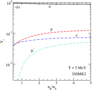
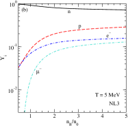
Figure 1: Particle fractions in finite-temperature $\beta$-equilibrated matter as functions of the baryon density $n_{B}$ (in units of nuclear saturation density $n_{0}$) for models DDME2 (a) and NL3 (b) at fixed temperature $T=5$ MeV.

Figure 2: The sum $p_{Fn}-p_{Fp}-p_{Fl}$, $l=\{e,\mu\}$, in zero-temperature $npe\mu$ matter for DDME2 and NL3 models. At $T=0$ the direct Urca process is only allowed in the regions where $p_{Fn}-p_{Fp}-p_{Fl}\leq 0$. Thus for DDME2 the direct Urca processes on electrons and muons are Boltzmann-suppressed at all the densities plotted, whereas for NL3 the threshold density for electronic and muonic Urca processes are $\approx 1.3n_{0}$ and $\approx 1.6n_{0}$, respectively. Above these the direct Urca processes are unsuppressed at low temperatures.

Particle fractions in $\beta$-equilibrated $npe\mu$ matter for the two parametrizations are shown in Fig. 1. The main difference between these two models is the larger proton and lepton fractions in the NL3 model. As a result, NL3 has direct electronic Urca threshold at $n_{B}\simeq 1.3n_{0}$ and muonic Urca threshold at $n_{B}\simeq 1.6n_{0}$, see Fig. 2, with $n_{0}$ being the nuclear saturation density which has the values $n_{0}=0.152$ fm^-3 for model DDME2 and $n_{0}=0.153$ fm^-3 for model NL3. The model DDME2 instead does not reach the direct Urca thresholds up to baryon density $n_{B}=5n_{0}$. In contrast to the case of neutrino-trapped matter Alford2021c , in the neutrino-transparent matter muons appear only above a certain baryon density $n_{B}\gtrsim n_{0}$, where the condition $\mu_{e}\geq m_{\mu}\simeq 106$ MeV is satisfied.

IV.1 Beta-equilibration rates

IV.1.1 Urca process rates

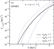
Figure 3: The rates for (a) neutron decay to an electron and (b) electron capture direct Urca processes as functions of the temperature for various densities for the DDME2 model. The dotted lines show the Urca process rates computed in Ref. Alford2019b within the approximation of nonrelativistic nucleons.

The direct Urca neutron-to-electron decay and electron-capture rates are shown in Figs. 3 and 4 as functions of the temperature for models DDME2 and NL3, respectively. The modified Urca contribution is discussed at the end of Sec. IV.2.

In the DDME2 model, the densities we study are all below the direct Urca threshold, so direct Urca rates are Boltzmann-suppressed at low temperatures. We see this in the rapid dropping off of both the neutron decay and electron capture rates as $T$ decreases. In fact, for densities $3n_{0}$ and $5n_{0}$ the suppression of the neutron decay rate is so strong that those curves are not visible on the plot.

Comparing panels (a) and (b) of Fig. 3 we see that the electron capture rate, although Boltzmann suppressed, is much faster than the neutron decay rate, and much less dependent on density. At saturation density, it is about three orders of magnitude faster than neutron decay and remains about the same as the density increases. Similar behavior of neutron decay rate was also found and discussed in Ref. Alford2021b .

Figure 3 shows in addition the neutron decay and electron capture rates computed in Ref. Alford2019b in the approximation of nonrelativistic nucleons. We see that the electron capture rates for nonrelativistic nucleons are smaller than the relativistic ones, the difference being as large as an order of magnitude at $n_{B}=5n_{0}$. The non-relativistic treatment of the neutron decay process, instead, strongly overestimates the rates above the saturation density, as the relativistic rates are strongly damped in this regime, as already mentioned above.

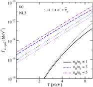
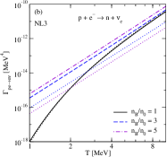
Figure 4: The rates for (a) neutron-to-electron decay and (b) electron capture direct Urca processes as functions of the temperature for various densities for the NL3 model. The dotted lines show the Urca process rates computed in Ref. Alford2019b within the approximation of nonrelativistic nucleons.

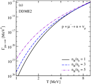
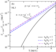
Figure 5: The muonic direct Urca processes rates for the DDME2 model (a) and the NL3 model (b). The neutron-to-muon decay is allowed only for the NL3 model above the direct Urca threshold (dotted lines).

Turning to the NL3 model, we see that at density $n_{B}=n_{0}$, which is below the direct Urca threshold, both neutron decay and electron capture rates show the expected Boltzmann suppression at low $T$, but the rates for NL3 are significantly faster than for DDME2. At higher densities, the direct Urca channel is open for NL3 where the neutron decay and the electron capture are almost equal and closely follow their low-temperature scaling $\Gamma_{n\to pe\bar{\nu}}=\Gamma_{pe\to n\nu}\propto T^{5}$ given by Eq. (12). The discrepancy between the relativistic and nonrelativistic calculations is within an order of magnitude also in this case. Note that the Urca process rates increase with the density in the case of NL3 model, but are non-monotonic in the case of DDME2.

The rates of muonic direct Urca processes are shown in Fig. 5. Panel (a) shows the results for muon capture for the model DDME2. The general behavior of the muon capture rates is similar to electron capture rates; however, quantitatively the muon capture rate is much smaller at low temperatures and becomes comparable to the electron capture above $T\geq 5$ MeV. The neutron-to-muon decay is strongly suppressed in the whole density range for the DDME2 model.

The muon capture rates for the NL3 model are shown in Fig. 5 (b). As in the case of DDME2, the muon capture rate is much slower than the electron capture rate at low temperatures $T\leq 5$ MeV below the direct Urca threshold, i.e., at $n_{B}=n_{0}$, whereas the electron and muon capture rates are almost equal above the threshold at all temperatures. We see also that the neutron-to-muon decay rate is nonvanishing only above the threshold where it is close to the muon capture rate. The difference between these rates increases with the temperature.

IV.1.2 Muon decay rate

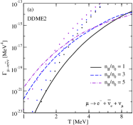
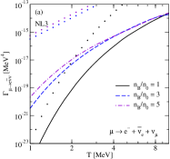
Figure 6: The muon decay rates as functions of the temperature for different densities for (a) the DDME2 model; (b) the NL3 model. The muon capture ($p\ +\mu^{-}\to n\ +\nu_{\mu})$ rates are shown by the dotted lines for comparison.

Figure 6 shows the muon decay rates given by Eq. (17). Muon decay is Boltzmann suppressed at low temperatures because, like neutron decay in the DDME2 model, at all densities, it is Pauli blocked for particles on their Fermi surfaces. A muon on its Fermi surface has just enough energy but insufficient momentum to create a final state electron on its Fermi surface, so it lacks the extra energy to create neutrinos to help with momentum conservation.

To decide whether we are in the slow lepton equilibration limit or the slow muon equilibration limit (29) we compare the muonic Urca rate to the electronic Urca and muon decay rates. The electron capture rates are always found to exceed the muon decay rates at least by an order of magnitude. In Fig. 6 where the Urca muon capture rates are shown by dotted lines, we see that the Urca muon capture rate is comparable to the muon decay rate only in the low temperature domain $T\lesssim 2$ MeV in the case of DDME2 model, indicating that the matter is in the slow-muon-equilibration regime, where the muonic component can be simply neglected when computing the bulk viscosity, as discussed in Sec. III. At higher temperatures $T\geq 3$ MeV the system is in the limit of slow lepton equilibration $\Gamma_{pe\to n\nu}\geq\Gamma_{p\mu\to n\nu}\gg\Gamma_{\mu\to e\bar{\nu}\nu}$. (Note that if one includes the modified Urca processes, then the muon decay rate will be always smaller than the sum of the direct and modified Urca rates.)

In the case of NL3 model, the lepton capture rates are always larger than the muon decay rates; they differ at least by an order of magnitude below the direct Urca threshold and at least three orders of magnitude above the threshold. Thus, the bulk viscosity of $npe\mu$ matter for the NL3 model should be computed under the slow-lepton-equilibration assumption in the whole temperature-density range of interest.

IV.2 Bulk viscosities

IV.2.1 Bulk viscosity of relativistic $npe$ matter

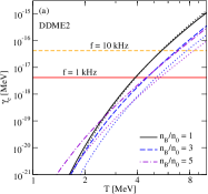
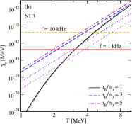
Figure 7: The $\beta$-relaxation rate $\gamma_{e}$ as a function of the temperature for fixed values of the density for (a) the DDME2 model; (b) the NL3 model. The dotted lines show the relaxation rates computed in Ref. Alford2019b within the approximation of nonrelativistic nucleons. The horizontal lines show where $\gamma_{e}=2\pi f$ for selected values of oscillation frequency $f=1$ kHz (solid lines) and $f=10$ kHz (dashed lines).

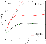
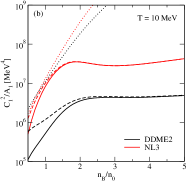
Figure 8: The susceptibility $C^{2}_{1}/A_{1}$ of $npe$ matter as a function of the baryon density for the DDME2 and NL3 models and fixed temperature (a) $T=1$ MeV and (b) $T=10$ MeV. The solid lines show the isothermal susceptibilities of relativistic matter, and the dotted lines show the isothermal susceptibilities computed in Ref. Alford2019b within the approximation of nonrelativistic nucleons. The green triangles in panel (a) show the result of Ref. Alford2019a for adiabatic susceptibility for the model DD2 at $T=1$ MeV. The dashed lines in panel (b) show the adiabatic susceptibilities at $T=10\,\text{MeV}$ as computed in Appendix B.2. At $T=1\,\text{MeV}$ (panel (a)) the difference between the isothermal and adiabatic susceptibilities is very small and is invisible in the plot.

In this subsection, we will assume that muons are absent and discuss the bulk viscosity of relativistic $npe$ matter given by Eq. (51). This improves on our previous treatments in Refs. Alford2019a ; Alford2019b where we used non-relativistic dispersion relations for nucleons in computing the rates of processes (but not in computing the background nuclear equilibrium) and on Ref. Alford2022 by showing the results for the NL3 density functional. For parallel developments which also used relativistic dispersion relations for nucleons with alternative background nuclear models see Ref. Alford:2023gxq .

The coefficients $\lambda_{l}$, defined by Eqs. (13), were computed by taking numerical derivatives of off-equilibrium Urca process rates. At densities $n_{B}\geq n_{0}$ we find approximately $\lambda_{l}\simeq c\Gamma_{pl\to n\nu}/T$, where the number $c$ varies in the range $0.3\leq c\leq 2$ (in the low-temperature limit $c\simeq 1.34$, see Eqs. (66) and (70)).

The susceptibility $A_{1}$ given by Eq. (37) is insensitive both to the temperature and the density, therefore the relaxation rate $\gamma_{e}=\lambda_{e}A_{1}$ scales as $\gamma_{e}\propto\Gamma_{pe\to n\nu}/T$, see Fig. 7. The relaxation rate $\gamma_{e}$ crosses the line of the constant angular frequency $\omega=2\pi\times 1\,\text{kHz}=4.14\cdot 10^{-18}$ MeV at temperatures $3\div 4$ MeV if the density is below the direct Urca threshold and around $T=2$ MeV for densities above the threshold, where $\gamma_{e}\propto T^{4}$. Consequently, the bulk viscosity attains its maximum at the temperature defined by the crossing. Compared to the nonrelativistic treatment, the full relativistic calculation predicts the point of the maximum of the bulk viscosity at lower temperatures, because it predicts faster equilibration rates.

Figure 8 shows the combination of (isothermal) susceptibilities $C_{1}^{2}/A_{1}$ relevant to the bulk viscosity (which in $npe$ matter takes the form of Eq. (51)) at two fixed temperatures $T=1$ MeV and $T=10$ MeV (panels (a) and (b), respectively). In full relativistic calculation $C_{1}^{2}/A_{1}$ is almost density-independent above $n_{B}=2n_{0}$ in contrast to its nonrelativistic counterpart which monotonically increases and strongly overestimates the bulk viscosity already at density $n_{B}=2n_{0}$. The temperature dependence of isothermal susceptibility $C_{1}^{2}/A_{1}$ is very weak in the range $1\leq T\leq 10$ MeV almost at all densities. The only exception is the density range below the nuclear saturation density. The green triangles in panel (a) show the results of Ref. Alford2019a for the DD2 model at $T=1$ MeV which were obtained by direct numerical differentiation of chemical imbalance $\mu_{\Delta}$. (Note that Refs. Alford2019a ; Alford2019b define the susceptibilities $A_{1}$ and $C_{1}$ via alternative expressions $A_{1}=-n_{B}^{-1}(\partial\mu_{\Delta}/\partial Y_{p})_{n_{B}}$, $C_{1}=n_{B}(\partial\mu_{\Delta}/\partial n_{B})_{Y_{p}}$). It is seen that the results of our analytic expressions for relativistic susceptibilities agree quite well with the results of Ref. Alford2019a .

For the sake of completeness, we compute also the adiabatic susceptibilities in addition to the isothermal ones. The dashed lines in panel (b) show the adiabatic susceptibilities as computed in Appendix B.2. (Note that, at low temperatures $T\simeq 1$ MeV the difference between the isothermal and adiabatic susceptibilities is very small and so is not visible on the left panel of the plot). We see that at high temperatures the adiabaticity enhances the susceptibility $C_{1}^{2}/A_{1}$ by a factor of a few at low densities $n_{B}\leq 2n_{0}$. Comparing the two panels of Fig. 8, we see also that the adiabatic susceptibilities are practically temperature-independent in the whole range of densities $0.5n_{0}\leq n_{B}\leq 5n_{0}$.

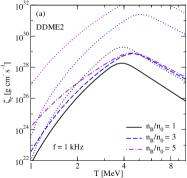
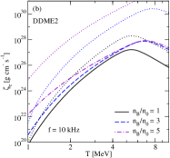
Figure 9: Each panel shows the bulk viscosity of relativistic $npe$ matter as a function of temperature for three values of baryon density for DDME2 model. The left panel is for oscillations of frequency $f=1$ kHz; the right panel is for $f=10$ kHz. The dotted lines show the results of Ref. Alford2019b obtained within the approximation of nonrelativistic nucleons.

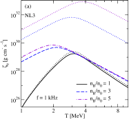
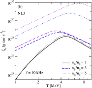
Figure 10: The bulk viscosity of relativistic $npe$ matter as a function of temperature for three values of baryon density for the NL3 model at (a) $f=1$ kHz; (b) $f=10$ kHz. The dotted lines show the results of Ref. Alford2019b obtained within the approximation of nonrelativistic nucleons.

Figures 9 and 10 show the temperature dependence of the bulk viscosity of $npe$ matter for DDME2 and NL3 models, respectively, computed according to Eq. (51). The results for the bulk viscosity in the isothermal case are shown for two frequencies $f=1$ kHz and $f=10$ kHz which bracket the typical range of frequencies of density oscillations in BNS mergers. As discussed above, for any given frequency $\zeta_{e}$ has a maximum at the temperature where $\omega=\gamma_{e}(T_{\rm max})$, and $T_{\rm max}$ increases with the frequency. The maximum value of the bulk viscosity for the given density decreases with the frequency as $\zeta_{e\rm max}=C_{1}^{2}/(A_{1}\omega)$. At temperatures below the resonant maximum, chemical equilibration is slower than density oscillations, i.e., $\gamma_{e}\ll\omega$, and the bulk viscosity drops rapidly as frequency rises $\zeta_{e}\propto\omega^{-2}$. At temperatures above the resonant maximum, chemical equilibration is faster than the oscillations and we have $\zeta_{e}=C_{1}^{2}/(A_{1}\gamma_{e})$, which is independent of the frequency.

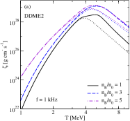
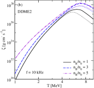
Figure 11: The bulk viscosity of relativistic $npe\mu$ matter as a function of temperature for three values of baryon density for the DDME2 model at (a) $f=1$ kHz; (b) $f=10$ kHz. The dotted lines show the bulk viscosities of relativistic $npe$ matter.

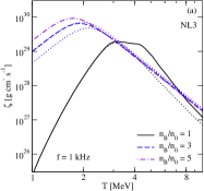
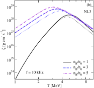
Figure 12: The bulk viscosity of relativistic $npe\mu$ matter as a function of temperature for three values of baryon density for the NL3 model at (a) $f=1$ kHz; (b) $f=10$ kHz. The dotted lines show the bulk viscosities of relativistic $npe$ matter.

In the case of the DDME2 model, in which direct Urca processes are kinematically forbidden at low temperatures (i.e., the relevant densities are always below the threshold density) the maximum of the bulk viscosity moves to a higher temperature as density increases from $n_{0}$ to $3n_{0}$. This is consistent with Fig. 7 where we see that for DDME2 $\gamma_{e}$ drops as density rises from $n_{0}$ to $3n_{0}$ at fixed $T$. In general, one expects Urca rates to increase with density (as seen for NL3) but this can be offset by other factors such as changes in the dispersion relations that affect the density of states at the Fermi surface. We already know from Fig. 3 that for DDME2 the Urca rates drop slightly with increasing density at $T\gtrsim 3$ MeV.

The NL3 model, in which particles near the Fermi surfaces can undergo direct Urca, shows the opposite behavior: the maximum is shifted to lower temperatures once the direct Urca threshold is achieved. This is expected since the rates rise with density because of increasing phase space at the Fermi surfaces, so $\gamma=1$ kHz is achieved at lower temperatures. Comparing these results with the ones obtained within the nonrelativistic approximation for nucleons we observe two characteristic features: (i) the maximum is shifted to lower temperatures in the relativistic calculation, the shift being larger above the direct Urca threshold; (ii) the approximation of nonrelativistic nucleons overestimates the bulk viscosity by orders of magnitude for DDME2 models and by an order of magnitude for NL3 model.

Note that, according to the susceptibilities shown in Fig. 8, the bulk viscosities computed in the adiabatic and isothermal cases will differ appreciably only below the saturation density.

IV.2.2 Bulk viscosity of relativistic $npe\mu$ matter

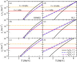
Figure 13: The quantities $n_{1}/n_{2}$, $d_{1}$ and $d_{2}$ entering in the expression of the bulk viscosity (46) as functions of the temperature for fixed values of density for the DDME2 model (left panels) and the NL3 model (right panels). The horizontal lines correspond to the squares of the oscillation frequencies fixed at $f=1$ kHz (solid lines) and $f=10$ kHz (dashed lines).

The bulk viscosity of relativistic $npe\mu$ matter computed in the slow-lepton equilibration limit (46) is shown in Figs. 11 and 12, for models DDME2 and NL3, respectively. The bulk viscosity of $npe$ matter $\zeta_{e}$ is shown for comparison by dotted lines. The qualitative behavior of $\zeta$ is similar to that of $\zeta_{e}$.

In the following, we first focus on the DDME2 density functional model (which does not reach the low-temperature Urca threshold at any density) and discuss first the low-temperature regime which is followed by a discussion of the high-temperature regime. At low temperatures, where $\lambda_{i}A_{j}\ll\omega$, we have $n_{1}/n_{2},d_{1},d_{2}\sim\lambda_{i}A_{j}\ll\omega^{2}$, and the bulk viscosity is given by $\zeta\simeq n_{2}/\omega^{2}=(\lambda_{e}C_{1}^{2}+\lambda_{\mu}C_{2}^{2})/\omega^{2}=\zeta_{e}+\zeta_{\mu}$ Haensel2000 . In this regime $\zeta_{\mu}$ is much smaller than $\zeta_{e}$, therefore the bulk viscosity of $npe\mu$ matter practically coincides with that of $npe$ matter. As shown above, in the case of DDME2 model the muons should be neglected in the evaluation of the bulk viscosity in the low-temperature sector, where all muonic processes are suppressed compared to the electronic Urca processes. However, because $\zeta_{\mu}\ll\zeta_{e}$ in this regime, the muonic contribution automatically drops, therefore the bulk viscosity of $npe\mu$ matter in the whole regime can be computed from Eq. (46).

At high temperatures, where equilibration is fast compared to the oscillation frequency, $\lambda_{i}A_{j}\gg\omega$, we approach the low-frequency limit where the bulk viscosity becomes frequency-independent and is equal to $\zeta=n_{1}/d_{1}^{2}\sim 1/\lambda_{i}$ which decreases with the temperature. In this regime, the bulk viscosity of $npe\mu$ matter exceeds the bulk viscosity of $npe$ matter by factors between 2.5 and 8 for the model DDME2. At intermediate temperatures, where $\lambda_{i}A_{j}\approx T$, the bulk viscosity obtains a maximum. However, as the quantities $n_{1}/n_{2},d_{1}$ and $d_{2}$ reach their maxima at slightly different temperatures, see Fig. 13, there is a broadened maximum or a “flattened” structure in the temperature dependence of $\zeta$, which is clearly pronounced at density $n_{B}=n_{0}$, see left panels of Figs. 11 and 12. The maximum of the bulk viscosity of $npe\mu$ matter is located at a slightly higher temperature as compared to the bulk viscosity of $npe$ matter.

In the case of NL3 model, the effect of the inclusion of muons on the bulk viscosity below the direct Urca threshold is the same as in the case of DDME2 model: muons enhance $\zeta$ by up to a factor of 3 at temperatures above the maximum, whereas they almost do not affect the bulk viscosity below the maximum. At densities $n_{B}=3n_{0}$ and $n_{B}=5n_{0}$, which are above the threshold, the electronic and muonic Urca rates are almost equal, see Figs. 4 and 5, resulting in almost equal contributions of electrons and muons to the bulk viscosity. Thus, to the left side of the maximum, where the bulk viscosity is proportional to the reaction rates, see Eq. (52), we have $\zeta\simeq\zeta_{e}+\zeta_{\mu}\simeq 2\zeta_{e}$. At higher temperatures, the total bulk viscosity is slightly smaller than that of $npe$ matter. Note also that above the direct Urca threshold, the inclusion of muons moves the location of the resonant maximum to smaller temperatures, whereas below the threshold the location of the maximum remains nearly unchanged.

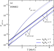
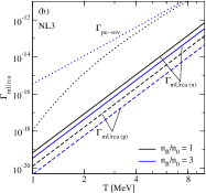
Figure 14: The rates of modified Urca process involving electrons at two fixed densities and for (a) DDME2 and (b) NL3 model. The direct Urca electron capture rates are shown by the dotted lines for comparison.

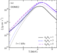
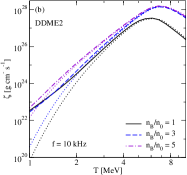
Figure 15: The bulk viscosity of relativistic $npe\mu$ matter with the inclusion of modified Urca processes for the DDME2 model at (a) $f=1$ kHz; (b) $f=10$ kHz. The dotted lines reproduce the bulk viscosities shown in Fig. 11 which were obtained neglected modified Urca processes.

For the sake of completeness, we also investigate how the modified Urca processes $N+n\rightarrow N+p+l^{-}+\bar{\nu}_{l}$ and $N+p+l^{-}\rightarrow N+n+{\nu}_{l}$, $N\in n,p$, affect the bulk viscosity (Fig. 15). For that purpose, we use the low-temperature modified Urca rates from Ref. Alford2019a . Note that there is no threshold for these processes.

The modified Urca rates for electronic processes for two models are shown in Fig. 14. Note that the low-temperature modified Urca rates are equal for neutron decay and electron capture processes when $\mu_{n}=\mu_{p}+\mu_{e}$. The rates of the muonic-modified Urca processes are very close to these and are not shown. The dotted lines show the rates of the direct Urca electron capture rates for comparison. Because the direct Urca neutron decay is strongly damped at densities below the direct Urca threshold, its rate is much smaller than that of the summed modified Urca rate at those densities. Below the direct Urca threshold and at moderate temperatures $T\geq 3$ MeV, the direct Urca lepton capture rates exceed the modified Urca rates by at least an order of magnitude. The modified Urca process rates become comparable to the direct Urca electron capture rates at $T\simeq 1.5$ MeV and the direct Urca muon capture rates at $T\simeq 3$ MeV for the model DDME2. Above the direct Urca threshold which is realized only in the case of NL3 model at densities $n_{B}\geq 1.5n_{0}$ both direct Urca rates are higher than the modified Urca rates by at least an order of magnitude. In the case of the NL3 model, the direct Urca electron capture rate is always at least two orders of magnitude larger than that of the modified Urca, whereas the direct muon capture rate becomes smaller than the modified process rate at $T\leq 2$ MeV below the threshold, e.g., at $n_{B}=n_{0}$. When the modified Urca processes are included, the summed Urca process rates are always much higher than the muon decay rates. Thus, the bulk viscosity of $npe\mu$ matter can be computed according to the slow-lepton-equilibration limit in the whole temperature-density range of interest. Figure 15 shows the bulk viscosity of the $npe\mu$ matter with the inclusion of modified Urca processes for the model DDME2. The bulk viscosity computed only with the direct Urca is shown for comparison with the dotted lines. We see that the inclusion of modified Urca processes becomes important at densities below the direct Urca threshold in the low-temperature regime $T\leq 3$ MeV. For NL3 model, the modified Urca processes do not have any significant impact on the bulk viscosity. Also, note that the modified Urca processes do not change the location of the maximum bulk viscosity.

IV.3 Damping of density oscillations

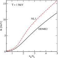
Figure 16: The incompressibility of nuclear matter for the DDME2 and NL3 models. The temperature is fixed at $T=1$ MeV.

Now we estimate the bulk viscous damping timescale in relativistic $npe\mu$ matter. The damping timescale is the decay time for a density oscillation and is given by Alford2018a ; Alford2019a ; Alford2020

$$\tau_{\zeta}=\frac{1}{9}\frac{Kn_{B}}{\omega^{2}\zeta},$$ (55)

where the incompressibility of nuclear matter is

$$K=9n_{B}\frac{\partial^{2}\epsilon}{\partial n_{B}^{2}},$$ (56)

and $\epsilon$ is the energy density. The incompressibility is plotted in Fig. 16. It is not sensitive to the temperature in the range $1\leq T\leq 10$ MeV, therefore the damping timescale shows temperature dependence inverse to that of the bulk viscosity and attains its minimum value at the temperature where the bulk viscosity has a maximum, see Figs. 17 and 18. The damping timescale is frequency-independent in the low-temperature regime, but is inversely proportional to $\omega^{2}$ in the high-temperature regime above the minimum. For the minimal value, we have $\tau_{\zeta}\propto 1/\omega$.

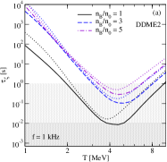
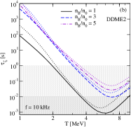
Figure 17: The damping timescale of oscillations as a function of temperature for various densities for the DDME2 model for (a) $f=1$ kHz and (b) $f=10$ kHz. The dotted lines show the damping timescales in $npe$ matter.

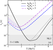
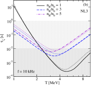
Figure 18: The damping timescale of oscillations as a function of temperature for various densities for the NL3 model for (a) $f=1$ kHz and (b) $f=10$ kHz. The dotted lines show the damping timescales for $npe$ matter.

As seen from Eq. (55), the dependence of $\tau_{\zeta}$ on the density arises from three factors: nuclear incompressibility, the baryon density, and the inverse bulk viscosity. Here we will use the bulk viscosities (plotted in Fig. 15 for the model DDME2) which include both direct and modified Urca processes. We see that the density dependence of the maximum bulk viscosity roughly follows $\zeta\propto n_{B}$, therefore the density dependence of minimal $\tau_{\zeta}$ just follows that of nuclear incompressibility. Thus, the damping timescales are smaller, and, therefore, the bulk viscous dissipation is more efficient at lower densities. This result is in contrast to our previous nonrelativistic treatment Alford2020 , where the damping timescale showed a decreasing behavior with the density as a result of the overestimation of the bulk viscosity at high densities.

The shaded regions in Figs. 17 and 18 show where the damping timescale becomes smaller than the short-term ($\simeq$10 ms, dark shaded areas) and long-term ($\simeq$1 s, lightly shaded areas) evolution timescales of a BNS merger remnant object. For a typical oscillation frequency $f=1$ kHz, the model DDME2 predicts that the bulk viscous damping would be marginally relevant in the short term, and noticeable for long-living remnants with $\tau_{\zeta}\geq 10$ ms at any density and in the temperature range $2\leq T\leq 10$ MeV. The damping timescale reaches its minimum at $n_{B}\leq n_{0}$ and $T\simeq 5$ MeV, where the damping time $\tau_{\zeta}$ reaches the short-term ($10\,$ms) evolution timescale. For higher frequencies, there is already a window of densities and temperatures where the damping timescales are shorter than the short-term evolution timescale of BNS mergers. For $f=10$ kHz the short-term damping is noticeable at densities $n_{B}\geq 3n_{0}$ and for temperatures between $4\leq T\leq 10$ MeV.

In the case of NL3 model, there is always a range of densities and temperatures where the bulk viscous damping time is comparable to the short-term evolution timescale. For oscillations of frequency $f=1$ kHz, the relevant parameter range is $n_{B}\lesssim 2n_{0}$ and 2 $\lesssim T\lesssim$ 5 MeV. The high-density region above the direct Urca threshold does not have a significant impact on the damping of density oscillations because the Urca processes are so fast that the system is not driven far from equilibrium. This result again differs from those of Ref. Alford2020 . At $f=10$ kHz, the damping timescale reaches down to the ms range also at high densities. On the long-term evolution timescale, the damping is efficient at all densities. Correspondingly, the range of temperatures where the bulk viscosity would play a role is larger than in the case of DDME2 model.

A comparison of Figs. 17 and 18 shows that the damping timescale is a few times shorter for model NL3 although the bulk viscosity for NL3 is larger by an order of magnitude. This is because NL3 matter is stiffer and has larger incompressibility, so density oscillations store more energy and this outweighs the larger bulk viscosity (see Eq. (55)).

The damping times shown in Figs. 17 and 18 are for isothermal oscillations. We have also performed calculations for adiabatic oscillations, and we find that at low densities $n_{B}\leq 2n_{0}$ and sufficiently high temperatures $T\geq 5$ MeV the adiabatic density oscillations have slightly shorter damping timescales. The maximal difference between adiabatic and isothermal nuclear incompressibilities is about 15% for DDME2 and 7% for NL3 models at $T=10$ MeV, see also Ref. Alford2019a .

V Conclusions

We studied the Urca-process-driven bulk viscosity of neutrino-transparent, relativistic $npe\mu$ matter in the temperature range $1\leq T\leq 10$ MeV and density range $0.5n_{0}\leq n_{B}\leq 5n_{0}$ which is relevant for BNS mergers. This parallels (and complements) our recent work Alford2021c where similar calculations were performed for relativistic neutrino-trapped $npe\mu$ matter. Using the analytic expressions for the relativistic beta-equilibration rates derived in Ref. Alford2021c we compute numerically the direct Urca neutron decay and lepton capture process rates with two (DDME2 and NL3) EoS models within the relativistic density functional theory for nuclear matter.

Imposing the $\beta$-equilibrium conditions $\mu_{n}=\mu_{p}+\mu_{l}$, strictly valid at low temperatures, we find that in the case of DDME2 model, which does not allow for a low-temperature direct Urca process (as the proton fraction stays always below the threshold), the neutron decay rate is strongly suppressed as compared to the lepton capture rate in the whole temperature-density range of interest and is completely damped at high densities. The qualitative picture is similar in the case of NL3 model at densities below the direct Urca threshold, whereas at higher densities above the threshold the neutron decay and the lepton capture rates are almost equal. We also find that the previous nonrelativistic approximation Alford2019b underestimates the relativistic electron capture rates by factors from 1 to 10 depending on the density.

In contrast to the neutrino-trapped matter, where the beta-relaxation rates $\gamma_{e}$ were always higher than the typical frequencies of density oscillations, in the neutrino-transparent matter the relaxation rate resonates with the typical frequencies $1\leq f\leq 10$ kHz at a temperature that lies in the range $4\leq T\leq 7$ MeV for DDME2 and $2\leq T\leq 5$ MeV for NL3, the exact value depending on the density and oscillation frequency. As a result, the bulk viscosity reaches a resonant maximum at that temperature. As compared to the non-relativistic case, the location of the maximum is shifted to lower temperatures, the shift being larger at densities above the direct Urca threshold. We also find that, as noted in Ref. Alford2021c , the nonrelativistic treatment of nucleons strongly overestimates the maximal values of the bulk viscosity because of an overestimate of susceptibilities in the nonrelativistic approximation.

Another way in which this computation adds to earlier treatments is the proper inclusion of muonic weak-equilibrium reactions in the bulk viscosity. As in Ref. Alford2021c , we analyze the relative rates of electronic and muonic Urca processes as well as the rates of pure leptonic processes, which is the muon decay in this case. The muon decay rates are found to be smaller than the Urca process rates almost in the whole temperature-density range, therefore, the bulk viscosity of $npe\mu$ matter can be computed neglecting the muon decay process. Thus, the bulk viscosity arises from two independent equilibration channels (i.e., electronic and muonic Urca channels), which results in a “flattened” structure in the temperature dependence of the bulk viscosity, which is in contrast to the bulk viscosity of $npe$ matter with a single peak at low densities. The “flattened” structure is clearly seen in the left panels of Figs. 11, and 12, the relevant bulk viscosity being shown by solid lines corresponding to $n_{B}/n_{0}=1$. The bulk viscosity of $npe\mu$ matter is higher than that of $npe$ matter by factors from 2.5 to 8 above the maximum temperature if the density is below the direct Urca threshold. Above the threshold, we find $\zeta\simeq 2\zeta_{e}$ below the maximum and $\zeta\lesssim\zeta_{e}$ above the maximum.

Using the results of the bulk viscosity we estimate the bulk viscous damping times of density oscillations for frequencies $f=1$ kHz and $f=10$ kHz. The damping timescale has a minimum as a function of temperature between $5\leq T\leq 7$ MeV (DDME2 model) and $2\leq T\leq 5$ MeV (NL3 model) for various densities.

For a typical frequency $f=1$ kHz, the DDME2 model predicts that the bulk viscous damping would be efficient only for long-living remnants with $\tau_{\zeta}\geq 10$ ms at any density and in the temperature range $2\leq T\leq 10$ MeV. The damping timescale reaches its minimum at $n_{B}\leq n_{0}$ and $T\simeq 5$ MeV, where $\tau\simeq 10$ ms reaches the short-term evolution timescale. For higher frequencies, there is already a window of densities and temperatures where the damping timescales are shorter than the short-term evolution timescale of mergers. For $f=10$ kHz the short-term damping is efficient at densities $n_{B}\geq 3n_{0}$ and for temperatures between $4\leq T\leq 10$ MeV.

In the case of NL3 model there is always a range of densities and temperatures where the bulk viscous damping is efficient within the short-term evolution timescale. At $f=1$ kHz the relevant parameter range is $n_{B}\leq 2n_{0}$ and 2 $\leq T\leq$ 5 MeV. The high-density region above the direct Urca threshold does not have a significant impact on the damping of density oscillations (in contrast to findings of Ref. Alford2020 ). At $f=10$ kHz the damping timescale reaches down to the ms range also at high densities. On the long-term evolution timescale, the damping is efficient at all densities. Correspondingly, the range of temperatures where the bulk viscosity would play a role is larger.

Our results for the bulk viscosity are most useful for estimating the damping of small-amplitude post-merger oscillations, see, e.g., Ref. Alford2020 . These results show the likely importance of bulk viscous damping arising from beta equilibration via weak interactions, and provide motivation for this physics to be included in simulations. Merger simulation groups are already exploring different approaches to the inclusion of beta equilibration, for example using the framework of the second-order Israel-Stewart relativistic hydrodynamics Camelio2023a ; Camelio2023b ; its relation to the one defined within the approach of Ref. Sawyer1989 and used here is discussed in Ref. Gavassino2021CQGra . Another possibility is to use an equation of state that includes the dependence on the particle fractions, and evolve those quantities, using the relevant reaction rates, in the simulation Most2022 .

It should be noted that complete second-order multi-fluid formulations of relativistic hydrodynamics will contain additional transport coefficients describing the relaxation of dissipative fluxes, in particular, the bulk-viscous flux; for review and references see Ref. Harutyunyan2023Symm .

Appendix A Low-temperature limit of Urca process rates

Here we present the details of the calculation of $\beta$-equilibration rates given by Eqs. (4) and (5). Writing the energy conservation in the form $\delta(k_{0}+p_{0}\pm k^{\prime}_{0}-p^{\prime}_{0})=\delta(\epsilon_{l}+\epsilon_{p}-\epsilon_{n}\pm\epsilon_{\bar{\nu}_{l}/\nu_{l}}-\mu_{\Delta_{l}})$, where $\epsilon_{i}$ are the energies of the particles computed from their (effective) chemical potentials (e.g., $\epsilon_{p}=\sqrt{p^{2}+m^{*2}_{p}}-\mu_{p}^{*}$), and substituting Eq. (6) into Eqs. (4) and (5) we obtain [$G=G_{F}\cos\theta_{c}(1+g_{A})$]

$$\Gamma_{n\to pl\bar{\nu}}(\mu_{\Delta_{l}}) = 2G^{2}\int d^{4}q\int\!\!\frac{d^{3}p}{(2\pi)^{3}p_{0}}\int\!\!\frac{d^{3}p^{\prime}}{(2\pi)^{3}p^{\prime}_{0}}\int\!\!\frac{d^{3}k}{(2\pi)^{3}k_{0}}\int\!\!\frac{d^{3}k^{\prime}}{(2\pi)^{3}k^{\prime}_{0}}(k\cdot p)(k^{\prime}\cdot p^{\prime})$$ (57)

$$\times \bar{f}(k)\bar{f}(p)\bar{f}(k^{\prime})f(p^{\prime})(2\pi)^{4}\delta^{(4)}(k+p-q)\delta^{(4)}(k^{\prime}-p^{\prime}+q)=2{G}^{2}\int d^{4}q\,I_{1}(q)\,I_{2}(q),$$

$$\Gamma_{pl\to n\nu}(\mu_{\Delta_{l}}) = 2G^{2}\int d^{4}q\int\!\!\frac{d^{3}p}{(2\pi)^{3}p_{0}}\int\!\!\frac{d^{3}p^{\prime}}{(2\pi)^{3}p^{\prime}_{0}}\int\!\!\frac{d^{3}k}{(2\pi)^{3}k_{0}}\int\!\!\frac{d^{3}k^{\prime}}{(2\pi)^{3}k^{\prime}_{0}}(k\cdot p)(k^{\prime}\cdot p^{\prime})$$ (58)

$$\times {f}(k){f}(p)\bar{f}(k^{\prime})\bar{f}(p^{\prime})(2\pi)^{4}\delta^{(4)}(k+p-q)\delta^{(4)}(-k^{\prime}-p^{\prime}+q)=2{G}^{2}\int d^{4}q\,\bar{I}_{1}(q)\,\bar{I}_{3}(q),$$

where

$$I_{1}(q) = \int\!\!\frac{d^{3}p}{(2\pi)^{3}p_{0}}\int\!\!\frac{d^{3}k}{(2\pi)^{3}k_{0}}\bar{f}(k)\bar{f}(p)\,(k\cdot p)\,(2\pi)^{4}\,\delta^{(4)}(k+p-q),$$ (59)

$$I_{2}(q) = \int\!\!\frac{d^{3}p^{\prime}}{(2\pi)^{3}p^{\prime}_{0}}\int\!\!\frac{d^{3}k^{\prime}}{(2\pi)^{3}k^{\prime}_{0}}\bar{f}(k^{\prime})f(p^{\prime})\,(k^{\prime}\cdot p^{\prime})\,\delta^{(4)}(k^{\prime}-p^{\prime}+q),$$ (60)

$$\bar{I}_{3}(q) = \int\!\!\frac{d^{3}p^{\prime}}{(2\pi)^{3}p^{\prime}_{0}}\int\!\!\frac{d^{3}k^{\prime}}{(2\pi)^{3}k^{\prime}_{0}}\bar{f}(k^{\prime})\bar{f}(p^{\prime})\,(k^{\prime}\cdot p^{\prime})\,\delta^{(4)}(-k^{\prime}-p^{\prime}+q),$$ (61)

and $\bar{I}_{1}$ is obtained from $I_{1}$ by replacing $\bar{f}(k)\bar{f}(p)\to{f}(k){f}(p)$. Here $\delta^{(4)}(k+p-q)=\delta({\bm{k}}+{\bm{p}}-{\bm{q}})\delta(\epsilon_{k}+\epsilon_{p}-\omega-\mu_{\Delta_{l}})$, and $\delta^{(4)}(\pm k^{\prime}-p^{\prime}+q)=\delta(\pm{\bm{k}}^{\prime}-{\bm{p}}^{\prime}+{\bm{q}})\delta(\pm\epsilon_{k^{\prime}}-\epsilon_{p^{\prime}}+\omega)$. The calculation of integrals (59)–(61) at finite temperatures was detailed in Ref. Alford2021b . Here we will derive only their low-temperature limit for the neutrino-transparent matter. In this limit, the antineutrino and neutrino distributions are zero in integrals $I_{2}$ and $\bar{I}_{3}$, respectively, the neutrino momentum in $\delta$-functions can be dropped and the magnitude of neutron momentum can be fixed to its value at the Fermi surface$p^{\prime}=p_{Fn}$. We then find

$$I_{2}(q) = (2\pi)^{-6}\int_{0}^{\infty}\!\!\frac{dp^{\prime}}{p^{\prime}_{0}}\int_{0}^{\infty}\!\!\frac{k^{\prime 2}dk^{\prime}}{k^{\prime}_{0}}\int d\Omega_{k^{\prime}}f(\epsilon_{p^{\prime}})\,(p^{\prime}_{0}k^{\prime}_{0}-{\bm{q}}\cdot{\bm{k}}^{\prime})\delta(\epsilon_{k^{\prime}}-\epsilon_{p^{\prime}}+\omega)\delta(q-p_{Fn})$$ (62)

$$= \frac{1}{(2\pi)^{5}}\delta(q-p_{Fn})\int_{0}^{\infty}\!\!k^{\prime 2}dk^{\prime}\,f(k^{\prime}+\omega)\frac{1}{p^{\prime}}\int_{-1}^{1}dy\,(p^{\prime}_{0}-qy)$$

$$= \frac{2}{(2\pi)^{5}}\delta(q-p_{Fn})\frac{\mu_{n}^{*}}{p_{Fn}}\int_{0}^{\infty}\!\!dk^{\prime}\,k^{\prime 2}f(k^{\prime}+\omega),$$

$$\bar{I}_{3}(q) = (2\pi)^{-6}\int_{0}^{\infty}\!\!\frac{dp^{\prime}}{p^{\prime}_{0}}\int_{0}^{\infty}\!\!\frac{k^{\prime 2}k^{\prime}}{k^{\prime}_{0}}\int d\Omega_{k^{\prime}}\bar{f}(\epsilon_{p^{\prime}})\,(p^{\prime}_{0}k^{\prime}_{0}-{\bm{q}}\cdot{\bm{k}}^{\prime})\delta(-\epsilon_{k^{\prime}}-\epsilon_{p^{\prime}}+\omega)\delta(q-p_{Fn})$$ (63)

$$= \frac{1}{(2\pi)^{5}}\delta(q-p_{Fn})\int_{0}^{\infty}\!\!k^{\prime 2}dk^{\prime}\bar{f}(\omega-\epsilon_{k^{\prime}})\frac{1}{p^{\prime}}\int_{-1}^{1}dy\,(p^{\prime}_{0}-qy)$$

$$= \frac{2}{(2\pi)^{5}}\delta(q-p_{Fn})\frac{\mu_{n}^{*}}{p_{Fn}}\int_{0}^{\infty}\!\!dk^{\prime}\,k^{\prime 2}{f}(k^{\prime}-\omega),$$

where $y$ is the cosine of the angle between $\bm{q}$ and $\bm{k}^{\prime}$, and we used $\epsilon_{k^{\prime}}=k^{\prime}_{0}=k^{\prime}$, as $m_{\nu}=\mu_{\nu}=0$. The low-$T$ limits of the integrals $I_{1}$ and $\bar{I}_{1}$ are given by Alford2021b

$$I_{1}(q) \simeq -\frac{{\omega}g(-{\omega})}{4\pi q}\,\theta(p_{Fl}+{p}_{Fp}-q)\theta(q-|p_{Fl}-{p}_{Fp}|)\,({p}_{Fp}^{2}+p_{Fl}^{2}+2\mu_{l}\mu_{p}^{*}-q^{2}),$$ (64)

$$\bar{I}_{1}(q) \simeq \frac{{\omega}g({\omega})}{4\pi q}\,\theta(p_{Fl}+{p}_{Fp}-q)\theta(q-|p_{Fl}-{p}_{Fp}|)\,({p}_{Fp}^{2}+p_{Fl}^{2}+2\mu_{l}\mu_{p}^{*}-q^{2}).$$ (65)

Then for the rates (57) and (58) we obtain

$$\Gamma_{n\to pl\bar{\nu}/pl\to n\nu} = 2{G}^{2}4\pi\frac{\mu_{n}^{*}}{p_{Fn}}\int_{-\infty}^{\infty}\!\!\!d\omega\int_{0}^{\infty}\!\!\!q^{2}dq\,\frac{\mp\omega g(\mp{\omega})}{4\pi q}\theta(p_{Fl}+{p}_{Fp}-q)\theta(q-|p_{Fl}-{p}_{Fp}|)$$ (66)

$$\times({p}_{Fp}^{2}+p_{Fl}^{2}+2\mu_{l}\mu_{p}^{*}-q^{2})\frac{2}{(2\pi)^{5}}\delta(q-p_{Fn})\int_{0}^{\infty}\!\!dk^{\prime}\,k^{\prime 2}f(k^{\prime}\pm\omega)$$

$$= \frac{{G}^{2}T^{5}}{8\pi^{5}}\mu_{n}^{*}\theta(p_{Fl}+{p}_{Fp}-p_{Fn})({p}_{Fp}^{2}+p_{Fl}^{2}+2\mu_{l}\mu_{p}^{*}-p_{Fn}^{2})\int_{-\infty}^{\infty}\!\!\!dy\,(\mp y)g(\mp{y})\int_{0}^{\infty}\!\!dx\,x^{2}f(x\pm y)$$

$$= \frac{\alpha}{2}{G}^{2}T^{5}\mu_{n}^{*}\theta(p_{Fl}+{p}_{Fp}-p_{Fn})({p}_{Fp}^{2}+p_{Fl}^{2}+2\mu_{l}\mu_{p}^{*}-p_{Fn}^{2}),$$

where $\alpha=3\left[\pi^{2}\zeta(3)+15\zeta(5)\right]/16\pi^{5}\simeq 0.0168$. In the limit of nonrelativistic nucleons we keep only the term $2\mu_{l}\mu_{p}^{*}$ in the brackets and, approximating $\mu_{N}^{*}\approx m_{N}^{*}$, we obtain

$$\Gamma_{n\to pl\bar{\nu}}=\Gamma_{pl\to n\nu}=\alpha m_{n}^{*}m_{p}^{*}\mu_{l}{G}^{2}T^{5}\theta(p_{Fl}+{p}_{Fp}-p_{Fn}),$$ (67)

which coincides with the results of Refs. Haensel2000 ; Yakovlev2001 ; Alford2018b ; Alford2019a ; Alford2019b if the lepton mass is neglected, i.e., $\mu_{l}=p_{Fl}$.

If matter is out of chemical equilibrium, i.e., $\mu_{\Delta_{l}}\neq 0$, one should replace $\omega\to\omega+\mu_{\Delta_{l}}$ in Eq. (64) and (65) as implied by the energy $\delta$-function after Eq. (61). Then the derivatives of (66) with respect to $\mu_{\Delta_{l}}$ at $\mu_{\Delta_{l}}=0$ are given by

$$\frac{\partial\Gamma_{n\to pl\bar{\nu}}}{\partial\mu_{\Delta_{l}}}\bigg{|}_{\mu_{\Delta_{l}}=0} = \frac{{G}^{2}T^{5}}{8\pi^{5}}\mu_{n}^{*}\theta(p_{Fl}+{p}_{Fp}-p_{Fn})({p}_{Fp}^{2}+p_{Fl}^{2}+2\mu_{l}\mu_{p}^{*}-p_{Fn}^{2})$$ (68)

$$\times\frac{\partial}{\partial\mu_{\Delta_{l}}}\int_{-\infty}^{\infty}\!\!\!dy\,(-\bar{y})g(-\bar{y})\int_{0}^{\infty}\!\!dx\,x^{2}f(x+y)$$

$$= \frac{{G}^{2}T^{4}}{8\pi^{5}}\mu_{n}^{*}\theta(p_{Fl}+{p}_{Fp}-p_{Fn})({p}_{Fp}^{2}+p_{Fl}^{2}+2\mu_{l}\mu_{p}^{*}-p_{Fn}^{2})$$

$$\times\int_{-\infty}^{\infty}\!\!\!dy\,[1+g({y})][1-{y}g({y})]\int_{0}^{\infty}\!\!dx\,x^{2}f(x+y),$$

$$-\frac{\partial\Gamma_{pl\to n\nu}}{\partial\mu_{\Delta_{l}}}\bigg{|}_{\mu_{\Delta_{l}}=0} = -\frac{{G}^{2}T^{5}}{8\pi^{5}}\mu_{n}^{*}\theta(p_{Fl}+{p}_{Fp}-p_{Fn})({p}_{Fp}^{2}+p_{Fl}^{2}+2\mu_{l}\mu_{p}^{*}-p_{Fn}^{2})$$ (69)

$$\times\frac{\partial}{\partial\mu_{\Delta_{l}}}\int_{-\infty}^{\infty}\!\!\!dy\,\bar{y}g(\bar{y})\int_{0}^{\infty}\!\!dx\,x^{2}f(x-y)$$

$$= \frac{{G}^{2}T^{4}}{8\pi^{5}}\mu_{n}^{*}\theta(p_{Fl}+{p}_{Fp}-p_{Fn})({p}_{Fp}^{2}+p_{Fl}^{2}+2\mu_{l}\mu_{p}^{*}-p_{Fn}^{2})$$

$$\times\int_{-\infty}^{\infty}\!\!\!dy\,g({y})[{y}(1+g({y}))-1]\int_{0}^{\infty}\!\!dx\,x^{2}f(x-y),$$

where $\bar{y}=y+\mu_{\Delta_{l}}/T$. The two-dimensional integrals in these expressions are the same and are equal to $17\pi^{4}/120$, therefore

$$\lambda_{l}=\left(\frac{\partial\Gamma_{n\to pl\bar{\nu}}}{\partial\mu_{\Delta_{l}}}-\frac{\partial\Gamma_{pl\to n\nu}}{\partial\mu_{\Delta_{l}}}\right)\bigg{|}_{\mu_{\Delta_{l}}=0}=\frac{17}{480\pi}{G}^{2}T^{4}\mu_{n}^{*}\theta(p_{Fl}+{p}_{Fp}-p_{Fn})({p}_{Fp}^{2}+p_{Fl}^{2}+2\mu_{l}\mu_{p}^{*}-p_{Fn}^{2}).$$ (70)

In the limit $\mu_{N}^{*}\simeq m_{N}^{*}\gg p_{FN}$, these results lead to

$$\lambda_{l}=\frac{17}{240\pi}m_{n}^{*}m_{p}^{*}\mu_{l}{G}^{2}T^{4}\theta(p_{Fl}+{p}_{Fp}-p_{Fn}),$$ (71)

which is consistent with previous nonrelativistic calculations of Refs. Haensel1992PhRvD ; Haensel2000 ; Alford2019a ; Alford2019b .

Appendix B Computation of susceptibilities

B.1 Isothermal susceptibilities

To compute the isothermal susceptibilities $A_{ij}^{T}=\frac{\partial\mu_{i}}{\partial n_{j}}\big{|}_{T}$ we use the following formula for the particle densities

$$n_{i}=\frac{1}{\pi^{2}}\int_{0}^{\infty}\!p^{2}dp\,[f_{i}(p)-f^{*}_{i}(p)],$$ (72)

where $f_{i}(p)$ and ${f}^{*}_{i}(p)$ are the distribution functions for particles and antiparticles, respectively. To compute first the nucleon susceptibilities we differentiate the left and right sides of Eq. (72) with respect to $n_{j}$ at constant temperature and use the relations

$$\frac{\partial f_{i}}{\partial n_{j}}\bigg{|}_{T} = -f_{i}(1-f_{i})\frac{1}{T}\left(\frac{m^{*}}{E_{p}}\frac{\partial m^{*}}{\partial n_{j}}-\frac{\partial\mu^{*}_{i}}{\partial n_{j}}\right),$$ (73)

$$\frac{\partial{f}^{*}_{i}}{\partial n_{j}}\bigg{|}_{T} = -{f}^{*}_{i}(1-{f}^{*}_{i})\frac{1}{T}\left(\frac{m^{*}}{E_{p}}\frac{\partial m^{*}}{\partial n_{j}}+\frac{\partial\mu^{*}_{i}}{\partial n_{j}}\right),$$ (74)

to obtain

$$\delta_{ij}=-\left(\frac{\partial m^{*}}{\partial n_{j}}\right){I}_{i}^{1,0}+\left(\frac{\partial\mu^{*}_{i}}{\partial n_{j}}\right){I}_{i}^{0,0},$$ (75)

where $m^{*}\equiv m_{n}^{*}=m_{p}^{*}$ is a short-hand notation for effective nucleon mass, $E_{p}=\sqrt{m^{*2}+p^{2}}$, and

$$I^{q,s}_{i}=\frac{1}{\pi^{2}T}\int_{0}^{\infty}\!p^{2}dp\left(\frac{m^{*}}{E_{p}}\right)^{q}\Big{[}z_{pi}^{s}\,f_{i}(1-f_{i})+(-1)^{q+s}\,{z}_{pi}^{*s}\,{f}^{*}_{i}(1-\bar{f}_{i})\Big{]},$$ (76)

with $z_{pi}=(E_{p}-\mu^{*}_{i})/T$, ${z}^{*}_{pi}=(E_{p}+\mu^{*}_{i})/T$ (the integrals with $s\neq 0$ will be used in the next subsection). Recall that all derivatives above are computed at $T={\rm const}$. Using the relation $\mu^{*}_{i}=\mu_{i}-g_{\omega}\omega_{0}-g_{\rho}\rho_{03}I_{3i}-\Sigma_{r}$ and the equations for vector meson mean fields

$$g_{\omega}\omega_{0}=\left(\frac{g_{\omega}}{m_{\omega}}\right)^{2}(n_{n}+n_{p}),\qquad g_{\rho}\rho_{03}=\frac{1}{2}\left(\frac{g_{\rho}}{m_{\rho}}\right)^{2}(n_{p}-n_{n}),$$ (77)

we obtain

$$B_{ij}\equiv\frac{\partial\mu^{*}_{i}}{\partial n_{j}}\bigg{|}_{T}=A_{ij}^{T}-\left(\frac{g_{\omega}}{m_{\omega}}\right)^{2}\left[1+\frac{2n_{B}}{g_{\omega}}\frac{\partial g_{\omega}}{\partial n_{B}}\right]-I_{3i}\left(\frac{g_{\rho}}{m_{\rho}}\right)^{2}\left[I_{3j}+\frac{n_{n}-n_{p}}{n_{0}}a_{\rho}\right]-\frac{\partial\Sigma_{r}}{\partial n_{j}}.$$ (78)

Next, we use the following equation for the scalar mean field

$$g_{\sigma}\sigma=m-m^{*}=-\frac{g_{\sigma}}{m_{\sigma}^{2}}\frac{\partial U(\sigma)}{\partial\sigma}+\frac{1}{\pi^{2}}\left(\frac{g_{\sigma}}{m_{\sigma}}\right)^{2}\sum_{i=n,p}\int_{0}^{\infty}p^{2}dp\,\frac{m^{*}}{E_{p}}\!\left[f_{i}(p)+{f}^{*}_{i}(p)\right],$$ (79)

to obtain (up to terms $\partial g_{\sigma}/\partial n_{B}$ which are small in the regime of interest and can be neglected)

$$\frac{\partial m^{*}}{\partial n_{j}}=-\frac{1}{m_{\sigma}^{2}}\frac{\partial^{2}U(\sigma)}{\partial\sigma^{2}}\frac{\partial m^{*}}{\partial n_{j}}+\left(\frac{g_{\sigma}}{m_{\sigma}}\right)^{2}\left(\frac{\partial m^{*}}{\partial n_{j}}\right)\left({I}_{n}^{2,0}+{I}_{p}^{2,0}\right)-\left(\frac{g_{\sigma}}{m_{\sigma}}\right)^{2}\left(B_{nj}{I}_{n}^{1,0}+B_{pj}{I}_{p}^{1,0}\right)$$

$$-\left(\frac{g_{\sigma}}{m_{\sigma}}\right)^{2}\left(\frac{\partial m^{*}}{\partial n_{j}}\right)\sum_{i=n,p}\frac{1}{\pi^{2}}\int_{0}^{\infty}\!\!dp\,\frac{p^{4}}{E_{p}^{3}}\!\left[f_{i}(p)+{f}^{*}_{i}(p)\right].$$ (80)

Introducing the short-hand notations

$$\tilde{I}_{i}={I}_{i}^{2,0}-\frac{1}{\pi^{2}}\int_{0}^{\infty}\!\!dp\,\frac{p^{4}}{E_{p}^{3}}\!\left[f_{i}(p)+{f}^{*}_{i}(p)\right],\qquad I_{\sigma}=\left(\frac{m_{\sigma}}{g_{\sigma}}\right)^{2}\left(1+\frac{1}{m_{\sigma}^{2}}\frac{\partial^{2}U}{\partial\sigma^{2}}\right),$$ (81)

and

$$\gamma=\frac{1}{\tilde{I}_{n}+\tilde{I}_{p}-I_{\sigma}},$$ (82)

we obtain

$$\frac{\partial m^{*}}{\partial n_{j}}=\gamma(B_{nj}{I}_{n}^{1,0}+B_{pj}{I}_{p}^{1,0}).$$ (83)

Substituting this into Eq. (75) we obtain the following equations for coefficients $B_{ij}$

$$B_{ij}{I}_{i}^{0,0}-\gamma\left(B_{nj}{I}_{n}^{1,0}+B_{pj}{I}_{p}^{1,0}\right){I}_{i}^{1,0}=\delta_{ij}.$$ (84)

In the case of $i\neq j$ we find from Eq. (84)

$$B_{np}=\gamma B_{pp}\frac{I_{p}^{1,0}I_{n}^{1,0}}{I_{n}^{0,0}-\gamma\left(I_{n}^{1,0}\right)^{2}},\qquad B_{pn}=\gamma B_{nn}\frac{I_{n}^{1,0}I_{p}^{1,0}}{I_{p}^{0,0}-\gamma\left(I_{p}^{1,0}\right)^{2}}.$$ (85)

Substituting these expressions into Eq. (84) for $i=j$ we obtain

$$B_{nn}=\frac{I_{p}^{0,0}-\gamma\left(I_{p}^{1,0}\right)^{2}}{I_{n}^{0,0}I_{p}^{0,0}-\gamma I_{p}^{0,0}\left(I_{n}^{1,0}\right)^{2}-\gamma I_{n}^{0,0}\left(I_{p}^{1,0}\right)^{2}},\qquad B_{pp}=\frac{I_{n}^{0,0}-\gamma\left(I_{n}^{1,0}\right)^{2}}{I_{n}^{0,0}I_{p}^{0,0}-\gamma I_{p}^{0,0}\left(I_{n}^{1,0}\right)^{2}-\gamma I_{n}^{0,0}\left(I_{p}^{1,0}\right)^{2}},$$ (86)

and

$$B_{np}=B_{pn}=\frac{\gamma I_{p}^{1,0}I_{n}^{1,0}}{I_{n}^{0,0}I_{p}^{0,0}-\gamma I_{p}^{0,0}\left(I_{n}^{1,0}\right)^{2}-\gamma I_{n}^{0,0}\left(I_{p}^{1,0}\right)^{2}}.$$ (87)

Finally, substituting Eqs. (86) and (87) in Eq. (78) and recalling the definitions $A_{n}=A_{nn}-A_{pn}$, $A_{p}=A_{pp}-A_{np}$ we obtain for isothermal susceptibilites

$$A_{n}^{T}=\frac{I_{p}^{0,0}-\gamma I_{p}^{1,0}\left(I_{n}^{1,0}+I_{p}^{1,0}\right)}{I_{n}^{0,0}I_{p}^{0,0}-\gamma I_{p}^{0,0}\left(I_{n}^{1,0}\right)^{2}-\gamma I_{n}^{0,0}\left(I_{p}^{1,0}\right)^{2}}+\left(\frac{g_{\rho}}{m_{\rho}}\right)^{2}\left(\frac{1}{2}-\frac{n_{n}-n_{p}}{n_{0}}a_{\rho}\right),$$ (88)

$$A_{p}^{T}=\frac{I_{n}^{0,0}-\gamma I_{n}^{1,0}\left(I_{n}^{1,0}+I_{p}^{1,0}\right)}{I_{n}^{0,0}I_{p}^{0,0}-\gamma I_{p}^{0,0}\left(I_{n}^{1,0}\right)^{2}-\gamma I_{n}^{0,0}\left(I_{p}^{1,0}\right)^{2}}+\left(\frac{g_{\rho}}{m_{\rho}}\right)^{2}\left(\frac{1}{2}+\frac{n_{n}-n_{p}}{n_{0}}a_{\rho}\right).$$ (89)

For lepton susceptibilities we have simply $A_{l}^{T}=1/{I}_{l}^{0,0}$, $l=\{e,\mu\}$.

B.2 Adiabatic susceptibilities

The adiabatic susceptibilities can be obtained by using the following chain rule for partial derivatives

$$A_{ij}^{s}\equiv\frac{\partial\mu_{i}}{\partial n_{j}}\bigg{|}_{s}=\frac{\partial\mu_{i}}{\partial n_{j}}\bigg{|}_{T}+\frac{\partial\mu_{i}}{\partial T}\,\frac{\partial T}{\partial n_{j}}\bigg{|}_{s}=A_{ij}^{T}-\frac{\partial\mu_{i}}{\partial T}\left(\frac{\partial s}{\partial T}\right)^{-1}\frac{\partial s}{\partial n_{j}}\bigg{|}_{T},$$ (90)

where $s$ is the entropy per baryon

$$s=-\sum_{i}\frac{1}{\pi^{2}n_{B}}\int_{0}^{\infty}\!p^{2}dp\Big{[}f_{i}\ln f_{i}+(1-f_{i})\ln(1-f_{i})+{f}^{*}_{i}\ln{f}^{*}_{i}+(1-{f}^{*}_{i})\ln(1-{f}^{*}_{i})\Big{]},$$ (91)

where the summation goes over all particle species, i.e., nucleons, and leptons. In the second step in Eq. (90) we used the relation

$$\frac{\partial s}{\partial n_{j}}\bigg{|}_{T}=-\frac{\partial s}{\partial T}\,\frac{\partial T}{\partial n_{j}}\bigg{|}_{s},$$ (92)

which can be obtained if one applies an analogous to Eq. (90) chain rule to $s$. Note that all particle densities are assumed to be kept constant in the partial derivatives with respect to $T$ in Eq. (90).

From Eq. (91) we obtain

$$n_{B}\frac{\partial s}{\partial n_{j}}\bigg{|}_{T} = \sum_{i}\frac{1}{\pi^{2}}\int_{0}^{\infty}\!p^{2}dp\left[\frac{\partial f_{i}}{\partial n_{j}}\ln\frac{1-f_{i}}{f_{i}}+\frac{\partial{f}^{*}_{i}}{\partial n_{j}}\ln\frac{1-{f}^{*}_{i}}{{f}^{*}_{i}}\right]-s\frac{\partial n_{B}}{\partial n_{j}}\bigg{|}_{T}.$$ (93)

Substituting here Eqs. (73) and (83) for nucleons we obtain

$$n_{B}\frac{\partial s}{\partial n_{j}}\bigg{|}_{T} = -s+\sum_{N}\frac{1}{\pi^{2}T}\int_{0}^{\infty}\!p^{2}dp\,\biggl{\{}B_{ij}\left[z_{pi}\,f_{i}(1-f_{i})-{z}^{*}_{pi}\,{f}^{*}_{i}(1-{f}^{*}_{i})\right]$$ (94)

$$-\gamma\left(B_{nj}{I}_{n}^{1,0}+B_{pj}{I}_{p}^{1,0}\right)\frac{m^{*}}{E_{p}}\!\left[z_{pi}\,f_{i}(1-f_{i})+{z}^{*}_{pi}\,{f}^{*}_{i}(1-{f}^{*}_{i})\right]\biggr{\}}$$

$$= -s+\left(B_{nj}{I}^{0,1}_{n}+B_{pj}{I}^{0,1}_{p}\right)-\gamma\left(B_{nj}{I}_{n}^{1,0}+B_{pj}{I}_{p}^{1,0}\right)\left({I}^{1,1}_{n}+{I}^{1,1}_{p}\right),$$

where we used the identities $\ln(1-f_{i})/f_{i}=z_{pi}$, $\ln(1-{f}^{*}_{i})/{f}^{*}_{i}={z}^{*}_{pi}$, and recalled the definitions (76).

Substitutuing now $B_{ij}$ from Eqs. (86) and (87) in Eq. (94) we find

$$n_{B}\frac{\partial s}{\partial n_{n}}\bigg{|}_{T} = -s+\left(B_{nn}{I}^{0,1}_{n}+B_{pn}{I}^{0,1}_{p}\right)-\gamma\left(B_{nn}{I}_{n}^{1,0}+B_{pn}{I}_{p}^{1,0}\right)\left({I}^{1,1}_{n}+{I}^{1,1}_{p}\right)$$ (95)

$$= -s+\frac{I_{p}^{0,0}{I}^{0,1}_{n}-\gamma I_{p}^{1,0}\left(I_{p}^{1,0}{I}^{0,1}_{n}-I_{n}^{1,0}{I}^{0,1}_{p}\right)-\gamma I_{p}^{0,0}{I}_{n}^{1,0}\left({I}^{1,1}_{n}+{I}^{1,1}_{p}\right)}{I_{n}^{0,0}I_{p}^{0,0}-\gamma I_{p}^{0,0}\left(I_{n}^{1,0}\right)^{2}-\gamma I_{n}^{0,0}\left(I_{p}^{1,0}\right)^{2}},$$

$$n_{B}\frac{\partial s}{\partial n_{p}}\bigg{|}_{T} = -s+\frac{I_{n}^{0,0}{I}^{0,1}_{p}-\gamma I_{n}^{1,0}\left(I_{n}^{1,0}{I}^{0,1}_{p}-I_{p}^{1,0}{I}^{0,1}_{n}\right)-\gamma I_{n}^{0,0}{I}_{p}^{1,0}\left({I}^{1,1}_{n}+{I}^{1,1}_{p}\right)}{I_{n}^{0,0}I_{p}^{0,0}-\gamma I_{p}^{0,0}\left(I_{n}^{1,0}\right)^{2}-\gamma I_{n}^{0,0}\left(I_{p}^{1,0}\right)^{2}}.$$ (96)

For leptons we have

$$\frac{\partial f_{l}}{\partial n_{l}}\bigg{|}_{T}=\frac{f_{l}(1-f_{l})}{T{I}_{l}^{0,0}},\qquad\frac{\partial{f}^{*}_{l}}{\partial n_{l}}\bigg{|}_{T}=-\frac{{f}^{*}_{l}(1-{f}^{*}_{l})}{T{I}_{l}^{0,0}},$$ (97)

and

$$n_{B}\frac{\partial s}{\partial n_{l}}\bigg{|}_{T} = \frac{1}{\pi^{2}}\int_{0}^{\infty}\!p^{2}dp\left[\frac{\partial f_{l}}{\partial n_{l}}\ln\frac{1-f_{l}}{f_{l}}+\frac{\partial{f}^{*}_{l}}{\partial n_{l}}\ln\frac{1-{f}^{*}_{l}}{{f}^{*}_{l}}\right]\bigg{|}_{T}$$ (98)

$$= \frac{1}{\pi^{2}T{I}_{l}^{0,0}}\int_{0}^{\infty}\!p^{2}dp\left[z_{pl}\,f_{l}(1-f_{l})-{z}^{*}_{pl}\,{f}^{*}_{l}(1-{f}^{*}_{l})\right]=\frac{I^{0,1}_{l}}{{I}_{l}^{0,0}}.$$

Next, we compute the temperature derivatives. Differentiating the left and right sides of Eq. (72) with respect to $T$ at constant $n_{j}$ and exploiting the expressions

$$\frac{\partial f_{i}}{\partial T}=f_{i}(1-f_{i})\frac{1}{T}\left(z_{pi}+\frac{\partial\mu^{*}_{i}}{\partial T}\right),\qquad\frac{\partial{f}^{*}_{i}}{\partial T}={f}^{*}_{i}(1-{f}^{*}_{i})\frac{1}{T}\left({z}^{*}_{pi}-\frac{\partial\mu^{*}_{i}}{\partial T}\right),$$ (99)

we obtain

$$\frac{\partial\mu_{i}}{\partial T}\simeq\frac{\partial\mu^{*}_{i}}{\partial T}=-\frac{{I}_{i}^{0,1}}{{I}_{i}^{0,0}},$$ (100)

where we took into account that the nucleon masses and mesonic mean fields are almost independent of the temperature. Then from Eqs. (91), (99) and (100) we find

$$n_{B}\frac{\partial s}{\partial T} = \sum_{i}\frac{1}{\pi^{2}}\int_{0}^{\infty}\!p^{2}dp\left[\frac{\partial f_{i}}{\partial T}\ln\frac{1-f_{i}}{f_{i}}+\frac{\partial\bar{f}_{i}}{\partial T}\ln\frac{1-\bar{f}_{i}}{\bar{f}_{i}}\right]$$ (101)

$$= \sum_{i}\frac{1}{\pi^{2}T}\frac{\partial\mu^{*}_{i}}{\partial T}\int_{0}^{\infty}\!p^{2}dp\left[z_{pi}\,f_{i}(1-f_{i})-\bar{z}_{pi}\,\bar{f}_{i}(1-\bar{f}_{i})\right]$$

$$+ \sum_{i}\frac{1}{\pi^{2}T}\int_{0}^{\infty}\!p^{2}dp\left[z_{pi}^{2}\,f_{i}(1-f_{i})+\bar{z}_{pi}^{2}\,\bar{f}_{i}(1-\bar{f}_{i})\right]$$

$$= \sum_{k}\left[I^{0,2}_{k}-\frac{\left({I}_{k}^{0,1}\right)^{2}}{{I}_{k}^{0,0}}\right]\equiv S.$$

Then from Eqs. (90), (100) and (101) we find

$$A_{ij}^{s}=A_{ij}^{T}+\frac{n_{B}}{S}\frac{{I}_{i}^{0,1}}{{I}_{i}^{0,0}}\frac{\partial s}{\partial n_{j}}\bigg{|}_{T},$$ (102)

which leads to

$$A_{n}^{s} = A_{n}^{T}+\frac{n_{B}}{S}\left(\frac{{I}_{n}^{0,1}}{{I}_{n}^{0,0}}-\frac{{I}_{p}^{0,1}}{{I}_{p}^{0,0}}\right)\frac{\partial s}{\partial n_{n}}\bigg{|}_{T},$$ (103)

$$A_{p}^{s} = A_{p}^{T}-\frac{n_{B}}{S}\left(\frac{{I}_{n}^{0,1}}{{I}_{n}^{0,0}}-\frac{{I}_{p}^{0,1}}{{I}_{p}^{0,0}}\right)\frac{\partial s}{\partial n_{p}}\bigg{|}_{T},$$ (104)

$$A_{l}^{s} = A_{l}^{T}+\frac{1}{S}\left(\frac{I_{l}^{0,1}}{I_{l}^{0,0}}\right)^{2}.$$ (105)

Note that due to the second term in Eq. (90) there are additional cross-terms between different particle species, e.g., between baryons and leptons for adiabatic susceptibilities. However, these terms are found to be smaller than the diagonal terms in the whole regime of interest and can be neglected.

References

- (1) M. Oertel, M. Hempel, T. Klähn and S. Typel, Equations of state for supernovae and compact stars, Reviews of Modern Physics 89 (2017) 015007, [1610.03361].
- (2) A. Lovato, T. Dore, R. D. Pisarski, B. Schenke, K. Chatziioannou, J. S. Read et al., Long Range Plan: Dense matter theory for heavy-ion collisions and neutron stars, arXiv e-prints (2022) arXiv:2211.02224, [2211.02224].
- (3) A. Sedrakian, J. J. Li and F. Weber, Heavy baryons in compact stars, Progress in Particle and Nuclear Physics 131 (2023) 104041, [2212.01086].
- (4) V. Dexheimer, M. Mancini, M. Oertel, C. Providência, L. Tolos and S. Typel, Quick Guides for Use of the CompOSE Data Base, Particles 5 (2022) 346–360.
- (5) A. Perego, S. Bernuzzi and D. Radice, Thermodynamics conditions of matter in neutron star mergers, Eur. Phys. J. A 55 (2019) 124, [1903.07898].
- (6) M. Hanauske, J. Steinheimer, A. Motornenko, V. Vovchenko, L. Bovard, E. R. Most et al., Neutron Star Mergers: Probing the EoS of Hot, Dense Matter by Gravitational Waves, Particles 2 (2019) 44–56.
- (7) W. Kastaun, R. Ciolfi, A. Endrizzi and B. Giacomazzo, Structure of Stable Binary Neutron Star Merger Remnants: Role of Initial Spin, Phys. Rev. D96 (2017) 043019, [1612.03671].
- (8) S. Bernuzzi, D. Radice, C. D. Ott, L. F. Roberts, P. Moesta and F. Galeazzi, How loud are neutron star mergers?, Phys. Rev. D94 (2016) 024023, [1512.06397].
- (9) F. Foucart, R. Haas, M. D. Duez, E. O’Connor, C. D. Ott, L. Roberts et al., Low mass binary neutron star mergers: gravitational waves and neutrino emission, Phys. Rev. D93 (2016) 044019, [1510.06398].
- (10) K. Kiuchi, Y. Sekiguchi, K. Kyutoku and M. Shibata, Gravitational waves, neutrino emissions, and effects of hyperons in binary neutron star mergers, Class. Quant. Grav. 29 (2012) 124003, [1206.0509].
- (11) Y. Sekiguchi, K. Kiuchi, K. Kyutoku and M. Shibata, Gravitational waves and neutrino emission from the merger of binary neutron stars, Phys. Rev. Lett. 107 (2011) 051102, [1105.2125].
- (12) M. Ruiz, R. N. Lang, V. Paschalidis and S. L. Shapiro, Binary Neutron Star Mergers: A Jet Engine for Short Gamma-Ray Bursts, Astrophys. J. Lett. 824 (2016) L6, [1604.02455].
- (13) W. E. East, V. Paschalidis, F. Pretorius and S. L. Shapiro, Relativistic simulations of eccentric binary neutron star mergers: One-arm spir al instability and effects of neutron star spin, Phys. Rev. D 93 (2016) 024011, [1511.01093].
- (14) E. R. Most, L. J. Papenfort and L. Rezzolla, Beyond second-order convergence in simulations of magnetized binary neutron stars with realistic microphysics, Mon. Not. RAS 490 (2019) 3588–3600, [1907.10328].
- (15) A. Bauswein, N.-U. F. Bastian, D. B. Blaschke, K. Chatziioannou, J. A. Clark, T. Fischer et al., Identifying a First-Order Phase Transition in Neutron-Star Mergers through Gravitational Waves, Phys. Rev. Lett. 122 (2019) 061102, [1809.01116].
- (16) A. Endrizzi, D. Logoteta, B. Giacomazzo, I. Bombaci, W. Kastaun and R. Ciolfi, Effects of chiral effective field theory equation of state on binary neutron star mergers, Phys. Rev. D 98 (2018) 043015, [1806.09832].
- (17) R. Ciolfi, W. Kastaun, J. V. Kalinani and B. Giacomazzo, First 100 ms of a long-lived magnetized neutron star formed in a binary neutron star merger, Phys. Rev. D 100 (2019) 023005, [1904.10222].
- (18) A. Tsokaros, M. Ruiz, V. Paschalidis, S. L. Shapiro and K. Uryū, Effect of spin on the inspiral of binary neutron stars, Phys. Rev. D 100 (2019) 024061, [1906.00011].
- (19) L. Baiotti and L. Rezzolla, Binary neutron star mergers: a review of Einstein’s richest laboratory, Rept. Prog. Phys. 80 (2017) 096901, [1607.03540].
- (20) L. Baiotti, Gravitational waves from neutron star mergers and their relation to the nuclear equation of state, Progress in Particle and Nuclear Physics 109 (2019) 103714, [1907.08534].
- (21) J. A. Faber and F. A. Rasio, Binary Neutron Star Mergers, Living Reviews in Relativity 15 (2012) 8, [1204.3858].
- (22) M. G. Alford, L. Bovard, M. Hanauske, L. Rezzolla and K. Schwenzer, Viscous Dissipation and Heat Conduction in Binary Neutron-Star Mergers, Phys. Rev. Lett. 120 (2018) 041101, [1707.09475].
- (23) T. Celora, I. Hawke, P. C. Hammond, N. Andersson and G. L. Comer, Formulating bulk viscosity for neutron star simulations, Phys. Rev. D 105 (2022) 103016, [2202.01576].
- (24) E. R. Most, A. Haber, S. P. Harris, Z. Zhang, M. G. Alford and J. Noronha, Emergence of microphysical viscosity in binary neutron star post-merger dynamics, arXiv e-prints (2022) arXiv:2207.00442, [2207.00442].
- (25) G. Camelio, L. Gavassino, M. Antonelli, S. Bernuzzi and B. Haskell, Simulating bulk viscosity in neutron stars. I. Formalism, Phys. Rev. D 107 (2023) 103031, [2204.11809].
- (26) G. Camelio, L. Gavassino, M. Antonelli, S. Bernuzzi and B. Haskell, Simulating bulk viscosity in neutron stars. II. Evolution in spherical symmetry, Phys. Rev. D 107 (2023) 103032, [2204.11810].
- (27) P. Hammond, I. Hawke and N. Andersson, Impact of nuclear reactions on gravitational waves from neutron star mergers, Phys. Rev. D 107 (2023) 043023.
- (28) R. F. Sawyer, Bulk viscosity of hot neutron-star matter and the maximum rotation rates of neutron stars, Phys. Rev. D 39 (1989) 3804–3806.
- (29) M. G. Alford and S. P. Harris, Damping of density oscillations in neutrino-transparent nuclear matter, Phys. Rev. C 100 (2019) 035803, [1907.03795].
- (30) M. Alford, A. Harutyunyan and A. Sedrakian, Bulk viscosity of baryonic matter with trapped neutrinos, Phys. Rev. D 100 (2019) 103021, [1907.04192].
- (31) M. G. Alford and A. Haber, Strangeness-changing rates and hyperonic bulk viscosity in neutron star mergers, Phys. Rev. C 103 (2021) 045810, [2009.05181].
- (32) M. Alford, A. Harutyunyan and A. Sedrakian, Bulk viscosity from Urca processes: n p e matter in the neutrino-trapped regime, Phys. Rev. D 104 (2021) 103027, [2108.07523].
- (33) M. Alford, A. Harutyunyan and A. Sedrakian, Bulk Viscosity of Relativistic npe Matter in Neutron-Star Mergers, Particles 5 (2022) 361–376, [2209.04717].
- (34) M. G. Alford, A. Haber and Z. Zhang, Isospin Equilibration in Neutron Star Mergers, 2306.06180.
- (35) M. Alford, A. Harutyunyan and A. Sedrakian, Bulk Viscous Damping of Density Oscillations in Neutron Star Mergers, Particles 3 (2020) 500–517, [2006.07975].
- (36) S. L. Shapiro and S. A. Teukolsky, Black holes, white dwarfs and neutron stars. The physics of compact objects. WILEY‐VCH Verlag GmbH, 1983.
- (37) W. Greiner and B. Müller, Gauge Theory of Weak Interactions. Physics and Astronomy Online Library. Springer, 2000, pp. 30, 260.
- (38) M. G. Alford and S. P. Harris, equilibrium in neutron-star mergers, Phys. Rev. C 98 (2018) 065806, [1803.00662].
- (39) G. Guo, G. Martínez-Pinedo, A. Lohs and T. Fischer, Charged-Current Muonic Reactions in Core-Collapse Supernovae, Phys. Rev. D 102 (2020) 023037, [2006.12051].
- (40) M. G. Alford and G. Good, Leptonic contribution to the bulk viscosity of nuclear matter, Phys. Rev. C82 (2010) 055805, [1003.1093].
- (41) G. A. Lalazissis, T. Nikšić, D. Vretenar and P. Ring, New relativistic mean-field interaction with density-dependent meson-nucleon couplings, Phys. Rev. C 71 (2005) 024312.
- (42) G. A. Lalazissis, J. König and P. Ring, New parametrization for the Lagrangian density of relativistic mean field theory, Phys. Rev. C 55 (1997) 540–543, [nucl-th/9607039].
- (43) N. K. Glendenning, Compact stars: nuclear physics, particle physics, and general relativity. Springer, New York, N.Y., 2000.
- (44) S. Typel and H. H. Wolter, Relativistic mean field calculations with density-dependent meson-nucleon coupling, Nucl. Phys. A 656 (1999) 331–364.
- (45) M. G. Alford, A. Haber, S. P. Harris and Z. Zhang, Beta Equilibrium Under Neutron Star Merger Conditions, Universe 7 (2021) 399, [2108.03324].
- (46) P. Haensel, K. P. Levenfish and D. G. Yakovlev, Bulk viscosity in superfluid neutron star cores. I. Direct Urca processes in npemu matter, Astron.& Astrophys. 357 (2000) 1157–1169, [astro-ph/0004183].
- (47) L. Gavassino, M. Antonelli and B. Haskell, Bulk viscosity in relativistic fluids: from thermodynamics to hydrodynamics, Classical and Quantum Gravity 38 (2021) 075001, [2003.04609].
- (48) A. Harutyunyan and A. Sedrakian, Phenomenological Relativistic Second-Order Hydrodynamics for Multiflavor Fluids, Symmetry 15 (2023) 494, [2302.09596].
- (49) D. G. Yakovlev, A. D. Kaminker, O. Y. Gnedin and P. Haensel, Neutrino emission from neutron stars, Physics Reports 354 (2001) 1–155, [astro-ph/0012122].
- (50) P. Haensel and R. Schaeffer, Bulk viscosity of hot-neutron-star matter from direct URCA processes, Phys. Rev. D 45 (1992) 4708–4712.