Amplification in parametrically-driven resonators near instability based on Floquet theory and Green’s functions

Abstract

Here we use Floquet theory to calculate the response of parametrically-driven time-periodic systems near the onset of parametric instability to an added external ac signal or white noise. We provide new estimates, based on the Green’s function method, for the response of the system in the frequency domain. Furthermore, we write novel expressions for the power and the noise spectral densities. We validate our theoretical results by comparing our predictions for the specific cases of a single degree of freedom parametric amplifier and of the parametric amplifier coupled to a harmonic oscillator with the numerical integration results and with analytical approximate results obtained via the averaging method up to second order.

I Introduction

Amplification near bifurcation points has been studied since at least the 80’s with the publication of a seminal paper by Wiesenfeld and McNamara on small ac signal amplification near period-doubling bifurcations in nonlinear continuous dynamical systems Wiesenfeld and McNamara (1985). This work was later extended to account also for saddle-node, transcritical, pitchfork, and Hopf bifurcations Wiesenfeld and McNamara (1986). In these systems, a small ac signal is added to a nonlinear dynamical system that is on the verge of a local codimention-1 bifurcation. In their model a stable limit cycle solution of a nonlinear dynamical system is perturbed by the addition of a small ac signal. The dynamics of the response of the nonlinear system to this perturbation is equivalent to the dynamics of a parametric amplifier, i.e. of a linear parametrically driven system with an added ac drive. Hence, Floquet theory can be used to calculate the gain of the amplification. What they found is that the closer one is to the bifurcation point the greater the response of the nonlinear system. The complexity of the response is simplified by the fact that the gain becomes dominated by the contribution of a single Floquet exponent. This occurs because one of the Floquet exponents becomes zero or crosses the imaginary axis at the bifurcation point. The generic analytical framework they developed to estimate this response is based on this fact. In addition to the response to a small added ac perturbation, Wiesenfeld also analyzed the effect of noise near bifurcations in a paper with Jeffries Jeffries and Wiesenfeld (1985) and explained the effect of noisy precursors of bifurcation in a periodically driven p-n junction. In a subsequent paper, Ref. Wiesenfeld (1985a), he calculated estimates for the noise spectral density (NSD). Near the bifurcation point, he found that the NSD peak has a Lorentzian shape.

This concept of amplification near bifurcation points was very fruitful and spurred many applications and new ideas in very diverse fields such as Josephson bifurcation amplifiers Vijay et al. (2009), bifurcation-topology amplifiers Karabalin et al. (2011), tipping points in climate science Lenton (2011), and ultra-sensitive nanoresonator charge detectors Dash et al. (2021). To the author’s knowledge, however, quantitative applications of the theory have not been many.

Here we improve upon previous models so as to be able to predict quantitatively the peak values of the power spectrum density (PSD) or the NSD, without the need for rescaling the Lorenzian lineshape to fit experimental data near the onset of parametric instability. Furthermore, if one is not very close to the instability threshold, the Floquet exponents could be a complex conjugate pair in the case of a one-degree-of-freedom parametric amplifier as one can verify from the Liouville’s formula Wiesenfeld (1985b). This fact results in split peaks such as predicted theoretically and observed experimentally in Ref. Batista et al. (2022). These split peaks have also been observed in parametric resonators with very high quality factors J. M. L. Miller et al. (2020). As it is, Wiesenfeld et al theory cannot predict correctly these peak values and likely they cannot be normalized to fit the data. Here, we turn it more quantitative, with no need for rescaling the response to an ac drive when the dynamics is known. We point out that the main general assertions of their model remain intact, the only improvement lies on the quantitative estimates for the gain of the amplifier.

We believe that our theoretical contribution will make the generic model of amplification near bifurcation points proposed by Wiesenfeld et al more accurate and, thus, likely to be even more useful and more widely used than it presently is. In addition to this, we provide an expression for the Green’s function that is not present in their papers or elsewhere to the author’s knowledge. We already used approximate expressions for the time-domain Green’s function of the classical parametric resonator in Refs. Batista and R. S. N. Moreira (2011); Batista (2012), in which it was divided in two parts: a translationally invariant in time part and another that is not translationally invariant in time. We used this fact to obtain a more intuitive expression for the response of the parametric resonator to an added ac signal or white noise. Here, we extended our Fourier analysis as presented in Ref. Batista et al. (2022), based on the approximate averaging method, to the, in principle, exact Floquet theory result. Furthermore, the results for the response of the resonator to the drive and the NSD seem more intuitive physically than the ones provided in the literature. The response of the resonator is similar to a combination of Rayleigh and Raman scattering processes.

This paper is organized as follows: In Sec. II, we develop the theory. In subsection II.1, we present the basic facts about the time-evolution operator or the fundamental matrix of linear dynamical systems. In subsection II.2, we present our results on parametric amplification based on Floquet theory. In subsection II.3, we show our main results on the generalized Green’s functions of time-periodic non-autonomous dynamical systems. We also apply this method to obtain the PSD or the NSD when an external signal, an ac drive or a white noise, is added to the unperturbed parametrically-driven dynamical system. In Sec. III, we present and discuss our results. In Sec. IV, we draw our conclusions. In the Appendix, we present a proof of Floquet’s theorem just for completeness of this paper.

II Theory

II.1 Preliminary: The Fundamental matrix

Given the linear non-autonomous ordinary differential equation (ODE) system

$$\dot{x}=A(t)x,$$ (1)

in which $x\in\mathbb{R}^{N}$ and $A(t)$ is a $N\times N$ real matrix. The solution to this ODE system can be written as $x(t)=\Phi(t)x_{0}$, where $x(0)=x_{0}$ and $\Phi(0)=\mathbb{1}$. The $N\times N$ matrix $\Phi(t)$ obeys

$$\dot{\Phi}(t)=A(t)\Phi(t).$$

This time-evolution operator is known as the fundamental or monodromy matrix. It can be written as

$$\Phi(t)=\left[\bm{\phi_{1}(t)\;\phi_{2}(t)\;...\phi_{N}(t)}\right]$$ (2)

in which $\bm{\phi}_{k}$ is the $k$-th column. With this notation $\Phi_{jk}=\bm{\phi}_{kj}$ is the $j$-th element of column $\bm{\phi}_{k}$. Since the time evolution of $x(t)$ is unique, $\Phi(t)$ is always non-singular (i.e. invertible), therefore $\bm{\phi}_{k}$’s are linearly independent.

According to Floquet’s theorem (see the Appendix for the proof) if $A(t)$ is time periodic with period $T$, the fundamental matrix can be written as $\Phi(t)=P(t)e^{Bt}$, where $P(t+T)=P(t)$ is a periodic matrix. The eigenvalues $\Phi(T)=e^{BT}$ are called Floquet multipliers, while the eigenvalues of $B$ are usually called Floquet exponents. If $|v_{k}\rangle$ is a column eigenvector of $B$ with eigenvalue $\rho_{k}$, then $e^{BT}|v_{k}\rangle=e^{\rho_{k}T}|v_{k}\rangle$. Note that the Floquet multipliers $e^{\rho_{k}T}$ remain the same if $\rho_{k}$ is replaced by $\rho_{k}+2i\pi n/T$. To avoid uncertainty regarding this, we choose $\rho_{k}$ to be in the first Floquet zone, that is $-\pi/T<Im\rho_{k}\leq\pi/T$. Here, the eigenvectors $|v_{j}\rangle$ are columns and $\langle v_{k}|$ are rows. They are not just the transpose of one another, rather, they are dual to each other, in such a way that $\langle v_{k}|v_{j}\rangle=\delta_{ij}$. In general, the eigenvectors of the matrix $B$ are not orthogonal, so the relation of the vector basis, generated by $|v_{j}\rangle$’s, and the dual vector basis, generated by $\langle v_{k}|$, is similar to the relation between a lattice basis vectors and its reciprocal lattice basis vectors. In three dimensions, it is easy to construct the reciprocal lattice basis vectors from the lattice basis vectors. In higher dimensions, one can see that if the columns of a given matrix are the eigenvectors $|v_{j}\rangle$, the dual basis vectors are the rows of the inverse of this matrix. One should not confuse this notation with the one used in Eq. (2). From linear algebra, one knows that the $|v_{k}\rangle$’s form a complete basis set, i.e. $\sum_{k}|v_{k}\rangle\langle v_{k}|=\mathbb{1}$. Therefore,

$$\Phi(t) =P(t)e^{Bt}=\sum_{j}|v_{j}\rangle\langle v_{j}|P(t)\sum_{k}e^{\rho_{k}t}|v_{k}\rangle\langle v_{k}|=\sum_{j,k}e^{\rho_{k}t}\tilde{P}_{jk}(t)|v_{j}\rangle\langle v_{k}|,$$ (3)

where $\tilde{P}_{jk}(t)=\langle v_{j}|P(t)|v_{k}\rangle$. Hence, one obtains $\tilde{\Phi}_{jk}(t)\doteq\langle v_{j}|\Phi(t)|v_{k}\rangle=e^{\rho_{k}t}\tilde{P}_{jk}(t)$ , where the canonical basis vector $|n\rangle$ is a vector with 1 at the $n$-th position and zero elsewhere. On the other hand, we have $\Phi_{jk}=\langle j|\Phi(t)|k\rangle=\sum_{l,m}e^{\rho_{m}t}\tilde{P}_{lm}(t)\langle j|v_{l}\rangle\langle v_{m}|k\rangle$. Here, we used the tilde to differentiate from the canonical basis elements $\Phi_{jk}(t)\neq\tilde{\Phi}_{jk}(t)$. Similarly, we have

$$\Phi^{-1}(t) =e^{-Bt}P^{-1}(t)\doteq e^{-Bt}Q(t)=\sum_{j,k}e^{-\rho_{j}t}\tilde{Q}_{jk}(t)|v_{j}\rangle\langle v_{k}|$$ (4)

and $\tilde{\Phi}^{-1}_{jk}(t)=\langle v_{j}|\Phi^{-1}(t)|v_{k}\rangle=e^{-\rho_{j}t}\tilde{Q}_{jk}(t)$. Notice that the columns of the fundamental matrix can be written as

$$\bm{\phi}_{n}(t)=\Phi(t)|n\rangle=\sum_{j,k}e^{\rho_{k}t}\tilde{P}_{jk}(t)|v_{j}\rangle\langle v_{k}|n\rangle,$$ (5)

which is more complicated than the expression for $\bm{\phi}_{k}(t)$ given in references Wiesenfeld (1985a); Wiesenfeld and McNamara (1986).

II.2 Amplification near the onset of parametric instability

The solution of the inhomogeneous real $n$-dimensional ODE system

$$\dot{x}=A(t)x+f(t),$$ (6)

can be related to the solution of the homogeneous system of Eq. (39). Applying the transformation, $x(t)=\Phi_{0}(t)y(t)$, where $\dot{\Phi}_{0}(t)=A(t)\Phi_{0}(t)$, with initial conditions $\Phi_{0}(t_{0})=\mathbb{1}$. We obtain then

$$\Phi_{0}(t)\dot{y}=f(t).$$

Hence, we find

$$y(t)=y(t_{0})+\int_{t_{0}}^{t}\Phi_{0}^{-1}(t^{\prime})f(t^{\prime})dt^{\prime}$$

The solution $x(t)$ is given by

$$x(t)=\Phi_{0}(t)x(t_{0})+\Phi_{0}(t)\int_{t_{0}}^{t}\Phi_{0}^{-1}(t^{\prime})f(t^{\prime})dt^{\prime}$$ (7)

If the quiescent solution of Eq. (39) is stable, then for sufficiently large, that is $t>>t_{0}$, $\Phi_{0}(t)x(t_{0})\rightarrow 0$, and we can write

$$x(t)=\int_{t_{0}}^{t}\Phi_{0}(t)\Phi_{0}^{-1}(t^{\prime})f(t^{\prime})dt^{\prime}=\int_{t_{0}}^{t}P(t)e^{B(t-t^{\prime})}P^{-1}(t^{\prime})f(t^{\prime})dt^{\prime}=\int_{t_{0}}^{t}P(t)e^{B(t-t^{\prime})}Q(t^{\prime})f(t^{\prime})dt^{\prime}.$$ (8)

Hence, $G(t,t^{\prime})=\Phi_{0}(t)\Phi_{0}^{-1}(t^{\prime})=P(t)e^{B(t-t^{\prime})}Q(t^{\prime})$ is a generalization of a Green’s function. The $n$-th component of the vector $x(t)$ is given by

$$x_{n}(t) =\sum_{m}\int_{-\infty}^{t}G_{nm}(t,t^{\prime})f_{m}(t^{\prime})dt^{\prime}$$ (9)

$$=\sum_{jklm}\langle j|v_{k}\rangle\langle v_{k}|l\rangle P_{nj}(t)\int_{-\infty}^{t}e^{\rho_{k}(t-t^{\prime})}Q_{lm}(t^{\prime})f_{m}(t^{\prime})dt^{\prime},$$

where we chose $t_{0}=-\infty$. With this choice, we get rid of transients. We point out that the expression in Eq. (9) is different from the equivalent representation given in Ref. Wiesenfeld and McNamara (1986), specifically in Eq. (2.22) therein. It seems there was a confusion between the basis of Floquet eigenvectors, i.e. the eigenvectors of $B$ ($\{|v_{k}\rangle|\;k=1,2,...,N\}$) and the canonical basis ($\{|k\rangle|\;k=1,2,...,N\}$). Hence, the elements of the time domain Green’s function can be written as

$$G_{nm}(t,t^{\prime})=\sum_{jkl}\langle j|v_{k}\rangle\langle v_{k}|l\rangle P_{nj}(t)e^{\rho_{k}(t-t^{\prime})}Q_{lm}(t^{\prime}).$$ (10)

In what follows, we will focus on a special case of Eq. (6), the case in which $x(t)\in\mathbb{R}^{2}$ and $f_{1}(t)=0$ and $f_{2}(t)=F_{0}\cos(\omega_{s}t)$. We restrict our attention to the time evolution of

$$x_{1}(t)=\sum_{jkl}\langle j|v_{k}\rangle\langle v_{k}|l\rangle P_{1j}(t)\int_{-\infty}^{t}e^{\rho_{k}(t-t^{\prime})}Q_{l2}(t^{\prime})f_{2}(t^{\prime})dt^{\prime}=\sum_{jkl}\langle j|v_{k}\rangle\langle v_{k}|l\rangle P_{1j}(t)I_{kl}(t),$$ (11)

where

$$I_{kl}(t)=\int_{-\infty}^{t}e^{\rho_{k}(t-t^{\prime})}Q_{l2}(t^{\prime})f_{2}(t^{\prime})dt^{\prime}.$$ (12)

From the Floquet theorem, $P(t)=P(t+T)$ and $Q(t)=Q(t+T)$. Also, we assume that we are near (in parameter space) the first parametric instability region where $T=2\pi/\omega$. Therefore, we can write the Fourier series expansions of the periodic matrices

$$P(t)=\sum_{n=-\infty}^{\infty}p_{n}e^{in\omega t},$$ (13)

$$Q(t)=\sum_{n=-\infty}^{\infty}q_{n}e^{in\omega t}.$$

We notice that if the elements of the matrix $A(t)$ are real, then all the elements of $\Phi(t)$ are also real. Since $\Phi(T)=e^{BT}$, this implies that if $e^{BT}|v_{k}\rangle=\mu_{k}|v_{k}\rangle$, then we also have $e^{BT}|v_{k}\rangle^{*}=\mu_{k}^{*}|v_{k}\rangle^{*}$. Furthermore, we have $B|v_{k}\rangle=\rho_{k}|v_{k}\rangle$, where $\rho_{k}=T^{-1}\ln\mu_{k}$ and $B=\sum_{k}\rho_{k}|v_{k}\rangle\langle v_{k}|$ is a real matrix too. Hence, $e^{-Bt}$ is real as well. Therefore, $P(t)=\Phi(t)e^{-Bt}$ is real. In addition to that, $Q(t)=e^{Bt}\Phi^{-1}(t)$ is also a real matrix. Consequently, we find that $p_{-n}=p_{n}^{*}$ and $q_{-n}=q_{n}^{*}$. Using this last Fourier expansion, we can calculate the integral and find analytical expressions for the matrix elements $I_{kl}(t)$,

$$I_{kl}(t) =F_{0}\sum_{n=-\infty}^{\infty}q_{n,l2}\int_{-\infty}^{t}e^{\rho_{k}(t-t^{\prime})}e^{in\omega t^{\prime}}\cos(\omega_{s}t^{\prime})dt^{\prime}$$ (14)

$$=F_{0}\sum_{n=-\infty}^{\infty}\frac{q_{n,l2}e^{\rho_{k}t}}{2}\left[\dfrac{e^{[-\rho_{k}+i((n+1)\omega+\Delta\omega)]t}}{-\rho_{k}+i((n+1)\omega+\Delta\omega)}-\dfrac{e^{-[\rho_{k}+i((1-n)\omega+\Delta\omega)]t}}{\rho_{k}+i((1-n)\omega+\Delta\omega)}\right]$$

$$=F_{0}\sum_{n=-\infty}^{\infty}\frac{q_{n,l2}}{2}\left[\dfrac{e^{[i((n+1)\omega+\Delta\omega)]t}}{-\rho_{k}+i((n+1)\omega+\Delta\omega)}-\dfrac{e^{-i[(1-n)\omega+\Delta\omega]t}}{\rho_{k}+i((1-n)\omega+\Delta\omega)}\right],$$

where $\Delta\omega=\omega_{s}-\omega$. We are interested in studying the response near the onset of the parametric instability. This occurs when one of the Floquet exponents has a zero real part. In the special case of the parametrically-driven resonator both Floquet exponents are real. We obtain approximately

$$I_{kl}(t)\approx\frac{F_{0}}{2}\left[\dfrac{q_{1,l2}^{*}e^{i\Delta\omega t}}{-\rho_{k}+i\Delta\omega}-\dfrac{q_{1,l2}e^{-i\Delta\omega t}}{\rho_{k}+i\Delta\omega}\right]=-F_{0}Re\left\{\dfrac{q_{1,l2}e^{-i\Delta\omega t}}{\rho_{k}+i\Delta\omega}\right\}.$$ (15)

If we have $\rho_{2}<<\rho_{1}<0$, the terms with the Floquet exponent $\rho_{2}$ decay much faster. Hence, we find approximately

$$x_{1}(t) =-\frac{F_{0}}{2}\sum_{jkl}\langle j|v_{k}\rangle\langle v_{k}|l\rangle P_{1j}(t)\left[\dfrac{q_{1,l2}^{*}e^{i\Delta\omega t}}{\rho_{k}-i\Delta\omega}+\dfrac{q_{1,l2}e^{-i\Delta\omega t}}{\rho_{k}+i\Delta\omega}\right]$$ (16)

$$\approx a_{s}\cos[(\omega+\Delta\omega)t+\varphi_{s}]+a_{i}\cos[(\omega-\Delta\omega)t+\varphi_{i}]$$

From Eq. (13), we have $P_{1j}(t)\approx p_{1,1j}e^{i\omega t}+p_{-1,1j}e^{-i\omega t}$. Hence, we find the complex coefficients $\tilde{a}_{s}=a_{s}e^{i\varphi_{s}}$ and $\tilde{a}_{i}=a_{i}e^{i\varphi_{i}}$ to be given by

$$\tilde{a}_{s}= -F_{0}\sum_{jkl}\langle j|v_{k}\rangle\langle v_{k}|l\rangle\frac{p_{1,1j}q^{*}_{1,l2}}{\rho_{k}-i\Delta\omega}=-F_{0}\langle 1|p_{1}\sum_{k}\frac{|v_{k}\rangle\langle v_{k}|}{\rho_{k}-i\Delta\omega}q^{*}_{1}|2\rangle=-F_{0}\langle 1|p_{1}\left(B-i\Delta\omega\right)^{-1}q^{*}_{1}|2\rangle,$$ (17)

$$\tilde{a}_{i}= -F_{0}\sum_{jkl}\langle j|v_{k}\rangle\langle v_{k}|l\rangle\frac{p_{1,1j}q_{1,l2}}{\rho_{k}+i\Delta\omega}=-F_{0}\langle 1|p_{1}\sum_{k}\frac{|v_{k}\rangle\langle v_{k}|}{\rho_{k}+i\Delta\omega}q_{1}|2\rangle=-F_{0}\langle 1|p_{1}\left(B+i\Delta\omega\right)^{-1}q_{1}|2\rangle.$$

From this, we can find the amplitudes of the signal and idler peaks. The approximate amplitudes of the signal and idler peaks are, respectively,

$$a_{s}= F_{0}\left|\sum_{jkl}\langle j|v_{k}\rangle\langle v_{k}|l\rangle\frac{p_{1,1j}q^{*}_{1,l2}}{\rho_{k}-i\Delta\omega}\right|\approx\frac{F_{0}\left|\sum_{jl}\langle j|v_{1}\rangle\langle v_{1}|l\rangle p_{1,1j}q^{*}_{1,l2}\right|}{\sqrt{\rho_{1}^{2}+\Delta\omega^{2}}},$$ (18)

$$a_{i}= F_{0}\left|\sum_{jkl}\langle j|v_{k}\rangle\langle v_{k}|l\rangle\frac{p_{1,1j}q_{1,l2}}{\rho_{k}+i\Delta\omega}\right|\approx\frac{F_{0}\left|\sum_{jl}\langle j|v_{1}\rangle\langle v_{1}|l\rangle p_{1,1j}q_{1,l2}\right|}{\sqrt{\rho_{1}^{2}+\Delta\omega^{2}}}.$$

The envelope is given by

$$r(t) =\pm\sqrt{u(t)^{2}+v(t)^{2}},\mbox{ where}$$ (19)

$$u(t) =a_{s}\cos(\Delta\omega t+\varphi_{s})+a_{i}\cos(\Delta\omega t+\varphi_{i}),$$

$$v(t) =a_{s}\sin(\Delta\omega t+\varphi_{s})-a_{i}\sin(\Delta\omega t+\varphi_{i}).$$

II.3 The Green’s function and the noise spectral density

In this subsection we develop an alternative method to obtain the response of the non-autonomous system to an added signal that we believe is simpler than the method we used above. Using the Fourier series of Eq. (13), we can write the time-domain generalized Green’s function as

$$G(t,t^{\prime})=P(t)e^{B(t-t^{\prime})}Q(t^{\prime})=\sum_{n=-\infty}^{\infty}\sum_{m=-\infty}^{\infty}p_{n}e^{B(t-t^{\prime})}e^{i(nt+mt^{\prime})\omega}q_{m}.$$ (20)

We notice that it can be split in two parts

$$G(t,t^{\prime})=G_{0}(t-t^{\prime})+G_{p}(t,t^{\prime}),$$ (21)

a translationally invariant in time part, function of $t-t^{\prime}$, given by

$$G_{0}(t-t^{\prime})=\sum_{n=-\infty}^{\infty}p_{n}e^{B(t-t^{\prime})}e^{in\omega(t-t^{\prime})}q_{-n}=\sum_{n=-\infty}^{\infty}p_{n}\sum_{k}|v_{k}\rangle\langle v_{k}|q_{-n}e^{(\rho_{k}+in\omega)(t-t^{\prime})},$$ (22)

and another part, which is a function of both $t$ and $t^{\prime}$, given by

$$G_{p}(t,t^{\prime})=\sum_{n=-\infty}^{\infty}p_{n}\sum_{m=-\infty}^{\infty}{\!\!\!\!}^{{}^{\prime}}e^{B(t-t^{\prime})}e^{i\omega(nt+mt^{\prime})}q_{m}=\sum_{n=-\infty}^{\infty}p_{n}\sum_{m=-\infty}^{\infty}{\!\!\!\!}^{{}^{\prime}}\sum_{k}|v_{k}\rangle\langle v_{k}|q_{m}e^{\rho_{k}(t-t^{\prime})+i\omega(nt+mt^{\prime})},$$ (23)

where $\sum^{\prime}$ indicates that the summation omits $m=-n$. The Fourier transform of $G_{0}(t-t^{\prime})$ is

$$\tilde{G}_{0}(\nu) =\int_{-\infty}^{\infty}e^{i\nu\tau}G_{0}(\tau)d\tau=\int_{0}^{\infty}e^{i\nu\tau}G_{0}(\tau)d\tau=-\sum_{n=-\infty}^{\infty}p_{n}\left[B+i(\nu+n\omega)I\right]^{-1}q_{-n}$$ (24)

$$=-\sum_{n=-\infty}^{\infty}\sum_{k}\frac{p_{n}|v_{k}\rangle\langle v_{k}|q_{n}^{*}}{\rho_{k}+i(\nu+n\omega)},$$

where $\tau=t-t^{\prime}$. To lowest order approximation, it can be written as

$$\tilde{G}_{0}(\nu) \approx-p_{1}^{*}\left[B+i(\nu-\omega)I\right]^{-1}q_{1}-p_{1}\left[B+i(\nu+\omega)I\right]^{-1}q_{1}^{*}$$ (25)

$$=-\sum_{k}\frac{p_{1}^{*}|v_{k}\rangle\langle v_{k}|q_{1}}{\rho_{k}+i(\nu-\omega)}-\sum_{k}\frac{p_{1}|v_{k}\rangle\langle v_{k}|q_{1}^{*}}{\rho_{k}+i(\nu+\omega)}.$$

Below, we can write the Fourier transform of $x(t)$ given in Eq. (8), with $t_{0}=-\infty$, as

$$\tilde{x}(\nu) =\int_{-\infty}^{\infty}e^{i\nu t}\int_{-\infty}^{t}G_{0}(t-t^{\prime})f(t^{\prime})dt^{\prime}dt+\int_{-\infty}^{\infty}e^{i\nu t}\int_{-\infty}^{t}G_{p}(t,t^{\prime})f(t^{\prime})dt^{\prime}dt$$ (26)

$$=\tilde{G}_{0}(\nu)\tilde{f}(\nu)-\sum_{n=-\infty}^{\infty}p_{n}\sum_{m=-\infty}^{\infty}{\!\!\!\!}^{{}^{\prime}}\left[B+i(\nu+n\omega)I\right]^{-1}q_{m}\tilde{f}(\nu+(n+m)\omega)$$

$$=\tilde{G}_{0}(\nu)\tilde{f}(\nu)-\sum_{n=-\infty}^{\infty}p_{n}\sum_{m=-\infty}^{\infty}{\!\!\!\!}^{{}^{\prime}}\sum_{k}|v_{k}\rangle\langle v_{k}|q_{m}\frac{\tilde{f}(\nu+(n+m)\omega)}{\rho_{k}+i(\nu+n\omega)},$$

where we used the relation

$$\int_{-\infty}^{\infty}e^{i\nu t}\int_{-\infty}^{t}e^{\rho_{k}(t-t^{\prime})+i\omega(nt+mt^{\prime})}f(t^{\prime})dt^{\prime}dt=-\frac{\tilde{f}(\nu+(n+m)\omega)}{\rho_{k}+i(\nu+n\omega)}.$$ (27)

The dynamical system response with lowest order corrections due to parametric pumping is given by

$$\tilde{x}(\nu)\approx\tilde{G}_{0}(\nu)\tilde{f}(\nu)+\tilde{A}(\nu)\tilde{f}(\nu-2\omega)+\tilde{B}(\nu)\tilde{f}(\nu+2\omega),$$ (28)

where the coefficients are

$$\tilde{A}(\nu) =-p_{1}^{*}\left[B+i(\nu-\omega)I\right]^{-1}q_{1}^{*}=-\sum_{k}\frac{p_{1}^{*}|v_{k}\rangle\langle v_{k}|q_{1}^{*}}{\rho_{k}+i(\nu-\omega)},$$ (29)

$$\tilde{B}(\nu) =-p_{1}\left[B+i(\nu+\omega)I\right]^{-1}q_{1}=-\sum_{k}\frac{p_{1}|v_{k}\rangle\langle v_{k}|q_{1}}{\rho_{k}+i(\nu+\omega)}.$$

Note that, since $B$ is a real matrix, we have $\tilde{A}(-\nu)=\tilde{B}^{*}(\nu)$. The expression given in Eq. (26) is equivalent to the one obtained in Ref. Batista et al. (2022). While the previous expression is approximate, based on the 1st-order averaging method, and specific to the one-degree-of-freedom parametric resonator with added noise, the one proposed here is more general and exact, since it is a direct application of Floquet theory. The expression given in Eq. (28) is an approximation to Eq. (26) in which we throw out the higher harmonic terms. Even this approximation, as we shall see, is considerably more accurate than the equivalent averaging results. It is noteworthy to mention that the matrix format of equations (29) is more compact, easier, and faster to deal numerically than the equivalent ones with summations. The expressions in matrix format are better suited for modern programming languages with builtin vectorization such as Python with the Numpy library. Notice that the expression for $\tilde{x}(\nu)$ in Eq. (26) with $\tilde{G}_{0}(\nu)$ given by Eq. (24) remain invariant when $\rho_{k}$ is replaced by $\rho_{k}+in\omega$. On the other hand, the approximate expression given in Eq. (28) is not invariant under this transformation. In this approximation, one has to choose $\rho_{k}$ in the first Floquet zone.

For the case in which $N=2$ and the only nonzero term of $f(t)$ is $f_{2}(t)$, the response $\tilde{x}_{1}(\nu)$ is given by

$$\tilde{x}_{1}(\nu)=\tilde{G}_{0,12}(\nu)\tilde{f}_{2}(\nu)+\tilde{A}_{12}(\nu)\tilde{f}_{2}(\nu-2\omega)+\tilde{B}_{12}(\nu)\tilde{f}_{2}(\nu+2\omega),$$ (30)

where $\tilde{G}_{0,12}(\nu)=\langle 1|\tilde{G}_{0}(\nu)|2\rangle$, $\tilde{A}_{12}(\nu)=\langle 1|\tilde{A}(\nu)|2\rangle$, and $\tilde{B}_{12}(\nu)=\langle 1|\tilde{B}(\nu)|2\rangle$. In the case in which $f_{2}(t)=F_{0}\cos(\omega_{s}t+\varphi_{0})$, we obtain $\tilde{f}_{2}(\nu)=\pi F_{0}\left[\delta(\nu+\omega_{s})+\delta(\nu-\omega_{s})\right]$. Hence, we obtain

$$\tilde{x}_{1}(\nu) =\pi F_{0}\left\{\tilde{G}_{0,12}(\nu)\left[\delta(\nu+\omega_{s})+\delta(\nu-\omega_{s})\right]+\tilde{A}_{12}(\nu)\left[\delta(\nu-\omega+\Delta\omega)+\delta(\nu-2\omega-\omega_{s})\right]\right.$$ (31)

$$\left.+\tilde{B}_{12}(\nu)\left[\delta(\nu+2\omega+\omega_{s})+\delta(\nu+\omega-\Delta\omega)\right]\right\}.$$

From this, we obtain that the signal and idler amplitudes are given by

$$a_{s}=F_{0}\left|\tilde{G}_{0,12}(\omega_{s})\right|\mbox{ and }a_{i}=F_{0}\left|\tilde{A}_{12}(\omega_{i})\right|.$$ (32)

One can make the following analogy of the above process with scattering Huber et al. (2020). In Eq. (31), the first term on the right side corresponds to Rayleigh scattering, in which the scattering occured without exchange of energy. The other terms correspond to Raman scattering where the incoming photon scattered inelastically. When $\omega_{s}<\omega$, the photon scatters and gains energy from the pump corresponding to a Stokes Raman scattering process. When $\omega_{s}>\omega$, the photon scatters and loses energy to the pump what corresponds to a anti-Stokes Raman scattering process. Here we neglect the superharmonic terms.

The PSD, when $\Delta\omega\neq 0$, is given by

$$S_{x_{1}}(\nu)=\lim_{\Delta\nu\rightarrow 0^{+}}\int^{\nu+\Delta\nu}_{\nu-\Delta\nu}\dfrac{\langle\tilde{x}_{1}(-\nu)\tilde{x}_{1}(\nu^{\prime})\rangle}{2\pi}\;d\nu^{\prime}$$ (33)

$$\approx\frac{\pi F_{0}^{2}}{2}\left\{\left|\tilde{G}_{0,12}(\nu)\right|^{2}\left[\delta(\nu+\omega_{s})+\delta(\nu-\omega_{s})\right]+\left|\tilde{A}_{12}(\nu)\right|^{2}\delta(\nu-\omega_{i})+\left|\tilde{B}_{12}(\nu)\right|^{2}\delta(\nu+\omega_{i})\right\}$$

$$\approx\frac{\pi F_{0}^{2}}{2}\left\{\left|\tilde{G}_{0,12}(\omega_{s})\right|^{2}\left[\delta(\nu+\omega_{s})+\delta(\nu-\omega_{s})\right]+\left|\tilde{A}_{12}(\omega_{i})\right|^{2}\left[\delta(\nu-\omega_{i})+\delta(\nu+\omega_{i})\right]\right\},$$

where $\omega_{i}=\omega-\Delta\omega$ is the idler angular frequency. When $\Delta\omega=0$, $\tilde{x}_{1}(\nu)$ is given by

$$\tilde{x}_{1}(\nu)\approx\pi F_{0}\left\{\left[\tilde{G}_{0,12}(\omega)+A_{12}(\omega)\right]\delta(\nu-\omega)+\left[\tilde{G}_{0,12}(\omega)+A_{12}^{*}(\omega)\right]\delta(\nu+\omega)\right\}.$$ (34)

From this, we find that the PSD at degenerate parametric amplification can be written as

$$S_{x_{1}}(\nu) =\lim_{\Delta\nu\rightarrow 0^{+}}\int^{\nu+\Delta\nu}_{\nu-\Delta\nu}\dfrac{\langle\tilde{x}_{1}(-\nu)\tilde{x}_{1}(\nu^{\prime})\rangle}{2\pi}\;d\nu^{\prime}$$ (35)

$$\approx\frac{\pi F_{0}^{2}}{2}\left\{\left|\tilde{G}_{0,12}(\nu)+\tilde{A}_{12}(\omega)\right|^{2}\delta(\nu-\omega)+\left|\tilde{G}_{0,12}(\nu)+\tilde{A}_{12}^{*}(\omega)\right|^{2}\delta(\nu+\omega)\right\}.$$

In the case in which $\tilde{f}_{2}(\nu)=\tilde{r}(\nu)$, where $\tilde{r}(\nu)$ is a white noise with zero mean and the statistical average $\langle\tilde{r}(\nu)\tilde{r}(\nu^{\prime})\rangle=4\pi D\delta(\nu+\nu^{\prime})$, where $D$ is the noise level. We find that the NSD, as defined in Ref. Batista et al. (2022), is given by

$$S_{N}(\nu)=\lim_{\Delta\nu\rightarrow 0^{+}}\int^{\nu+\Delta\nu}_{\nu-\Delta\nu}\dfrac{\langle\tilde{x}_{1}(-\nu)\tilde{x}_{1}(\nu^{\prime})\rangle}{2\pi}\;d\nu^{\prime}=2D\left(\left|\tilde{G}_{0,12}(\nu)\right|^{2}+\left|\tilde{A}_{12}(\nu)\right|^{2}+\left|\tilde{B}_{12}(\nu)\right|^{2}\right).$$ (36)

III Numerical results and discussion

Here we apply the general theory developed in the previous section to two specific dynamical systems. The first one is a single parametric amplifier, whose equation of motion is given by

$$\ddot{x}=-x-\gamma\dot{x}+F_{p}\cos(2\omega t)x+F_{0}\cos(\omega_{s}t+\phi_{0}).$$ (37)

The second system is a parametric amplifier coupled to a harmonic oscillator with the following equations of motion

$$\ddot{x} =-\gamma_{1}\dot{x}-[1-F_{p}\cos(2\omega t)]x-\beta_{1}y+F_{0}\cos(\omega_{s}t+\phi_{0}),$$ (38)

$$\ddot{y} =-\gamma_{2}\dot{y}-\omega_{2}^{2}y-\beta_{2}x.$$

This model is the linearized version of the model proposed by Singh et al Singh et al. (2020) to study frequency-comb spectrum generation in parametrically-driven coupled mode resonators.

In Fig. 1, we show cyclostationary time series of the numerical integration of Eq. (37) compared with the predictions of Floquet theory given by the first term of Eq. (16), while the envelopes are given by Eq. (19). In these examples only the harmonics with $n=\pm 1$ are enough to give a very accurate description of the dynamics. We needed contributions from the both Floquet exponent terms to reach this very high agreement especially in the results of frames (a) and (c) which present larger detunings and one is not as close to the threshold of instability.

In Fig. 2, we show Floquet theory and numerical results of the signal and idler gains, based on Eq. (17), as a function of $\omega_{s}$ for the single parametric amplifier of Eq. (37). We point out that only the lowest terms of the Floquet theory expansion are enough to give a very accurate representation of the response of the parametric amplifier. There are only two slight disagreements on the far left side of frame (a) and on the far right side of frame (c) for the signal response. We show that this discrepancy disappears when we take into account the off-resonance terms in the Floquet theory expansion for $a_{s}$ and $a_{i}$ using the Green’s method given in Eq. (32).

In Fig. 3, we show Floquet theory and numerical results of the signal and idler gains, given by Eq. (17), as a function of $\omega_{s}$ for the coupled parametric amplifier model of Eq. (38). Again only the lowest terms of the Floquet theory expansion are enough to give a very accurate representation of the response of the parametric amplifier.

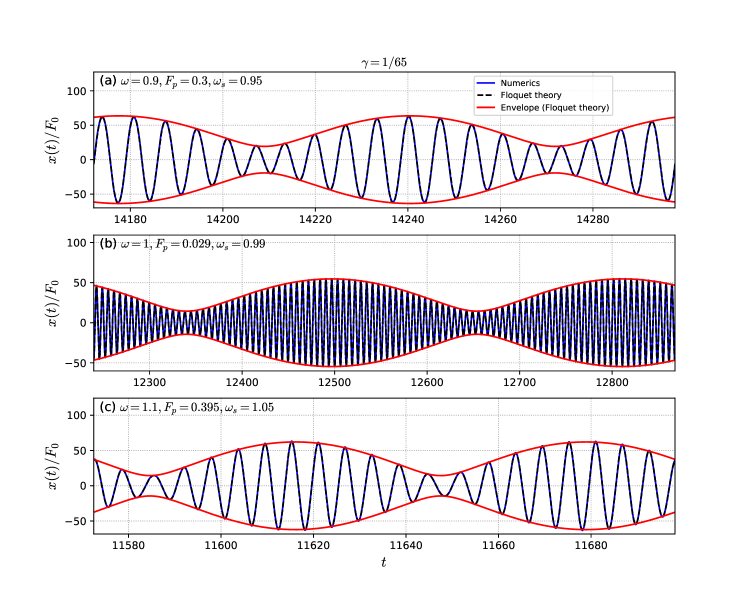
Figure 1: Single parametric amplifier model defined in Eq. (37). Comparison between a numerical time series and the corresponding envelope obtained from Floquet theory in Eq. (19). The amplification here is set in quasi-degenerate mode with all parameters indicated in the figure.

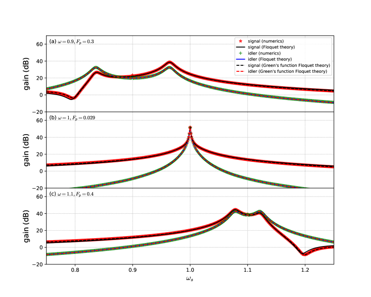
Figure 2: Floquet theory and numerical signal and idler response gains as a function of the ac drive angular frequency for the single parametric amplifier model defined in Eq. (37). The signal gain in dB scale is given by $20\log_{10}(a_{s}/F_{0})$ and the idler gain in dB is given by $20\log_{10}(a_{i}/F_{0})$. The amplitudes $a_{s}$ and $a_{i}$ obtained from Eq. (17) are represented by the full lines, while $a_{s}$ and $a_{i}$ obtained from Eq. (32) are shown by the dashed lines. In frames a) and c) the Floquet exponents are complex, what causes the split peaks in the signal and idler responses, whereas in frame b) they are real. In all frames $\gamma=1/65$.

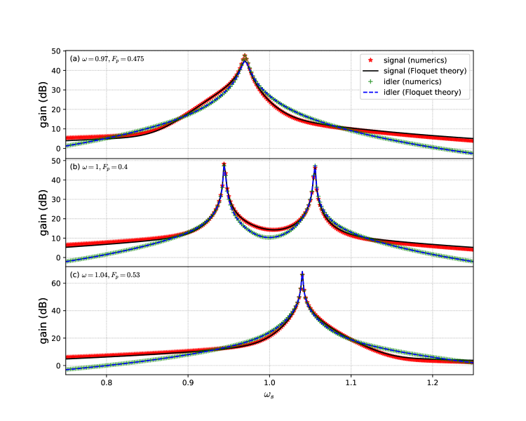
Figure 3: Coupled parametric amplifier model defined in Eq. (38). Theoretical signal and idler response gains for the two coupled resonators, one parametrically driven and the other harmonic. In frames a) and c) the Floquet exponents are real, whereas in frame b) they are complex, what causes the split peaks in the signal and idler responses. Common parameters used and not indicated in the figure are: $\gamma_{1}=\gamma_{2}=0.1$, $\omega_{2}=1.01$, $\beta_{1}=\beta_{2}=0.15$, and $\phi_{0}=0$.

In Fig. 4, we show the averaging method (first and second order approximations) and the Floquet theory results for the NSD $S_{N}$ of the parametric resonator with added noise given by the Eq. (36). Here we used the noise level $D=3.08\times 10^{-8}$ (in dimensionless units) and the quality factor $Q=65$. These values were obtained from the electronic circuit implementation of a parametric oscillator given in Ref. Batista et al. (2022). In this case, $x(t)$ has dimensions of voltage (measured in units of $V$) and the noise level has dimensions of squared voltage over frequency (measured in units of $V^{2}/Hz$). To transform our dimensionless $D$ to the experimental noise level, we divide it by $\omega_{0}$ the natural angular frequency of the resonator in units of $\mathrm{r}\mathrm{a}\mathrm{d}\mathrm{/}\mathrm{s}$ and multiply it by $\mathrm{V}^{2}$. The averaging method results are obtained from the approximations to the Green’s functions Fourier transforms. The first-order approximation to the frequency-domain response is given in Ref. Batista et al. (2022). The second-order approximation to the frequency-domain response is obtained from the time-domain GF given in Ref. Batista (2012). In this approximation, the functional form of the GF’s remains the same as in the first-order approximation, except that the parameters of the 2nd-order GF are obtained from a renormalization of the parameters of the 1st-order GF. We clearly see that the second-order averaging method results are substantially closer to the Floquet theory results of $S_{N}$. In frame (a), first-order averaging already gives a fairly accurate result with discrepancy of about 1 to 2 dBs, while in frame (c) first-order averaging is off by as far as about 6dB around $\nu=1.1$. There is a huge improvement when one goes to second-order averaging, where the error becomes lower that 1dB at the worst case. In frame(b), both averaging methods yield excellent agreements with the Floquet theory results.

By obtaining the NSD by independent methods, their mutual agreement indicates that the Floquet theory results proposed here are correct. Further improvement in the agreement could be obtained by going to higher orders of the averaging method, but the cost is high to justify the marginal improvement beyond second-order approximation. Another approach to verify our results is to use numerical integration of stochastic differential equations. But they are time consuming with very long time series and many integrations (over 1000) to yield satisfactory results, especially near narrow peaks due to resolution bandwidth limitations. On the other hand, the Floquet theory method proposed here for calculating $S_{N}$ could be used as a nontrivial benchmark to test stochastic differential equation integration methods of cyclostationary processes.

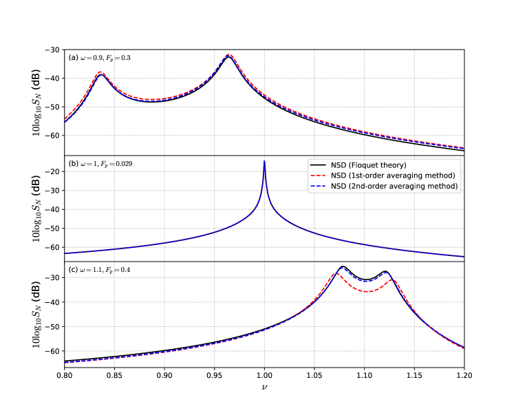
Figure 4: The parametrically-driven resonator NSD $S_{N}$ in dB. Comparison between Floquet theory predictions (dashed line), given by Eq. (36) and the approximate first-order averaging method (solid red line) for the NSD of a parametrically-driven resonator with added white noise. In frames a) and c), we have a parametric amplification of noise in which the Floquet exponents are a complex-conjugate pair, whereas in frame b), we have a parametric amplification in which the Floquet exponents are real. In all frames $\gamma=1/65$.

IV Conclusion

Here, we obtained the frequency-domain Green’s functions of parametrically-driven periodic dynamical systems using Floquet theory. From this, we wrote the Fourier transform of the response of the parametric amplifier to an added external drive. Near the parametric instability threshold, this response can be simplified to include only the contribution of a single real Floquet exponent that is closest to zero or of a complex conjugate pair of Floquet exponents whose real part is closest to zero. In this limit, the resulting expression for the response is thus considerably simplified. The calculated response of the parametrically-driven system to an added ac drive or to noise, as can be seen in Eq. (28), is more intuitive and simpler than equivalent ones in the literature. We achieved this by splitting the time-domain Green’s function in two pieces: one that is translationally invariant in time, i.e. dependent only on $t-t^{\prime}$ and the other that is independently a function of $t$ and $t^{\prime}$. This simple observation led to a better understanding of the frequency-domain behavior of the response of the parametrically excited dynamical system. Furthermore, we also provide an expression for the NSD (Eq. (36)) in parametrically-driven systems that is very accurate and extends our previous work Batista et al. (2022). To validate our model, we compared our results on PSD with numerical integration results for signal and idler gain and on NSD with the equivalent results based on the averaging method in the first and second order approximations. We obtained considerably better agreement of the excited system frequency-domain response between the second-order approximation and the Floquet theory results.

In addition to these results, we improved upon previous models by Wiesenfeld et al on amplification of small signals near bifurcation points and also on noisy precursors of bifurcations by making them more quantitative. Although, we did not investigate the effect of the several types of bifurcations on amplification, the results presented here are general enough to be able to apply to all of them. Furthermore, we believe that our contribution may help the development of amplifiers and sensors near bifurcation points such as parametrically-driven nano-mechanical resonators Lee et al. (2022) and Josephson parametric amplifiers Yamamoto et al. (2008).

We believe that in addition to the small signal amplification application, the theory developed here is also relevant to explaining the generation of frequency combs in parametrically-driven nonlinear dynamical systems Batista and Lisboa de Souza (2020). In several of these systems, the frequency-comb spectrum was experimentally observed to occur near bifurcation points Ganesan et al. (2018); Czaplewski et al. (2018). Hence, a better understanding of the linear behavior of these dynamical systems provided by the Green’s function method based on Floquet theory that we developed here may be relevant in guiding future developments in this field. This method may also be extended to investigate the linear response of limit cycles in nonlinear dynamical systems to added small ac perturbations or noise. In this way, one could calculate the amplification gain near several types of bifurcation points.

Appendix

For completeness, we present Floquet’s theorem adapted from Ref. Verhulst (1996).

Theorem (Floquet’s theorem).

Given the linear ODE system

$$\dot{x}=A(t)x,$$ (39)

in which $A(t)$ is a continuous periodic $n\times n$ matrix such that $A(t+T)=A(t)$. The fundamental matrix $\Phi(t)$ of this ODE system can be written as the matrix product

$$\Phi(t)=P(t)e^{Bt},$$ (40)

in which $P(t+T)=P(t)$ is periodic and $B$ is a constant $n\times n$ matrix.

Proof.

Since the Eq. (39) has a unique solution for any initial conditions, the fundamental matrix has an inverse. By differentiating the operator $\Phi(t)\Phi^{-1}(t)=\mathbb{1}$, we obtain

$$\frac{d\Phi^{-1}}{dt}=-\Phi^{-1}\frac{d\Phi}{dt}\Phi^{-1}=-\Phi^{-1}A(t)\Phi\Phi^{-1}=-\Phi^{-1}A(t).$$ (41)

Differentiating the operator $\Phi^{-1}(t)\Phi(t+T)$, we find

$$\frac{d}{dt}[\Phi^{-1}(t)\Phi(t+T)] = -\Phi^{-1}(t)A(t)\Phi(t+T)+\Phi^{-1}(t)A(t+T)\Phi(t+T)$$

$$= -\Phi^{-1}(t)A(t)\Phi(t+T)+\Phi^{-1}(t)A(t)\Phi(t+T)=0,$$

hence $\Phi^{-1}(t)\Phi(t+T)$ is a constant in time. This can be written as $\Phi^{-1}(t)\Phi(t+T)=\Phi(T)=C$, since $\Phi(0)=\mathbb{1}$. This implies that $\Phi(t+T)=\Phi(t)C$.

As we can always find a matrix $B$ such that $C=e^{BT}$ (see Lemma 7.1 of Ref. Hale (1969)), we find that

$$\Phi(t+T)e^{-B(t+T)}=\Phi(t)e^{BT}e^{-B(t+T)}=\Phi(t)e^{-Bt}.$$

This means that $P(t)\doteq\Phi(t)e^{-Bt}=P(t+T)$ is periodic. Hence, $\Phi(t)=P(t)e^{Bt}$. ∎