Ultrametric identities in glassy models of Natural Evolution

Abstract

Spin-glasses constitute a well-grounded framework for evolutionary models. Of particular interest for (some of) these models is the lack of self-averaging of their order parameters (e.g. the Hamming distance between the genomes of two individuals), even in asymptotic limits, much as like the behavior of the overlap between the configurations of two replica in mean-field spin-glasses. In the latter, this lack of self-averaging is related to peculiar fluctuations of the overlap, known as Ghirlanda-Guerra identities and Aizenman-Contucci polynomials, that cover a pivotal role in describing the ultrametric structure of the spin-glass landscape. As for evolutionary models, such identities may therefore be related to a taxonomic classification of individuals, yet a full investigation on their validity is missing. In this paper, we study ultrametric identities in simple cases where solely random mutations take place, while selective pressure is absent, namely in flat landscape models. In particular, we study three paradigmatic models in this setting: the one parent model (which, by construction, is ultrametric at the level of single individuals), the homogeneous population model (which is replica symmetric), and the species formation model (where a broken-replica scenario emerges at the level of species). We find analytical and numerical evidence that in the first and in the third model nor the Ghirlanda-Guerra neither the Aizenman-Contucci constraints hold, rather a new class of ultrametric identities is satisfied; in the second model all these constraints hold trivially. Very preliminary results on a real biological human genome derived by The 1000 Genome Project Consortium and on two artificial human genomes (generated by two different types neural networks) seem in better agreement with these new identities rather than the classic ones.

1 Introduction

1.1 The evolutionary interpretation of spin glasses

Spin glasses constitute a paradigmatic example of complex system Parisi1 ; Parisi2 ; TonRSB and their peculiar behavior is often evoked when describing some non-trivial phenomenologies occurring in disparate areas of Science, from several branches of Biology (e.g. neurology Amit ; Neuro2 ; Neuro3 , genomics Genomics1 ; Genomics2 , immunology Immunology1 ; Immunology2 ; BillPnas , ecology Ecology1 ; Ecology2 ; Sole ) to Sociology Social1 ; Social2 , Economics Economics1 ; Economics2 , Computer Science ComputerScience1 ; ComputerScience2 and more.

Here we will focus on the framework provided by spin-glass theory to Natural Evolution, which has attracted much interest in the past decades and nowadays represents an insightful and solid branch of modern disordered statistical mechanics. In this picture genomic randomness plays a crucial role; take for instance the adaptive walks approach, where Natural Evolution is modelled as a two-step stochastic process: $i.$ the genotype of a species undergoes random mutations, $ii.$ its newborns with higher fitness are preserved (see e.g. Kauffman ). Then, as pointed out by Eigen, the compromise between replication efficiency and frequency of mutations in evolutionary dynamics is conceptually close to the compromise between energy minimization and entropy maximization in statistical mechanics, moreover, the error threshold in the mutation rate in the former mimics the thermal noise of the latter Franz ; Tarazona . Also, to quantify the genetic variability within a population, we can introduce a proximity measure $q$ between pairs of individuals that plays like an order parameter (mirroring the replica overlap) and, just like in disordered systems, two distinct averages can be implemented, namely the population average (mirroring the thermal average) and the process average (mirroring the quenched average) DP1 . Therefore, one can consider the population-average of $q$, which in general depends on time, and inspect whether its average over a long time stretch exhibits vanishing fluctuations. If this is the case we have a self-averaging structure of the model (in such a way that its main features could be captured by the quasi-species limiting description), and, if not, we have a non-self-averaging structure, that is a hallmark of complex systems.

In this context it is also worth recalling Wright’s Adaptive Landscape (see e.g. 1932 ), Fisher’s Fundamental Theorem of Natural Selection and Kimura’s Neutral Theory Kimura which constitute fundamental steps Frank . Along these lines, the development of a disordered statistical mechanical theory for Natural Evolution was started by Leuthäusser Lede and Tarazona Tarazona and a spin-glass setting was pursued by Derrida, Higgs, Franz, Peliti, Sellitto, and Serva, just to name a few (see e.g. DP1 ; Franz ; Derrida2 ; Derrida3 ; Peliti2 ; Peliti-Darwin and references therein). More specifically, we recognize two classes of models: those where both random mutations and selective pressure are involved (also referred to as rugged landscape models) and those where evolution is driven only by random mutations (also referred to as flat landscape models). Reference models for the former are the P-spin-glass Kauffman , the random energy model (REM) Franz and the Hopfield model Tarazona , while for the latter we mention the One Parent Model (OPM) DP1 , the Homogeneous Population Model (HPM) Peliti2 , and the Specie Formation Model (SFM) Derrida2 ; Derrida3 . The OPM is asexuated and its order parameter lacks self-averaging, while its sexuated counterpart, the HPM, is self-averaging, unless a threshold in the similarity between the two genomes that are matching to reproduce is introduced and this case corresponds to the SFM. Notably, in the latter, the presence of a similarity threshold yields a persistent, spontaneous formation and extinction process at the level of species with consequent breakdown of self-averaging.

The behaviour of the order-parameter fluctuations in spin-glass models has been extensively studied, starting from the fully-connected Sherrington-Kirkpatrick (SK) model AC1 ; Barra0 ; CG1 ; GG1 , to its generalizations (see e.g., Barra2 ; DeSanctisFranz ; FranzLeone ; Burioni ; PCbook ; Dmitry0 ; ASS1 ; ASS2 ; Sollich ; Barra3 ; Bovier1 ; Bovier2 ; CG2 ; CG3 ; Chatter ; More1 ; More2 ; Tala and Sec. 1.2 for more details), including the rugged landscape models mentioned above. There, the order parameters are proved to be non-self-averaging and their momenta satisfy a class of non-trivial identities known as Ghirlanda-Guerra and Aizenman-Contucci (the latter are actually a family of identities that is a subset of the Ghirlanda-Guerra ones). Thus, in the context of Natural Evolution, the presence of both random mutation and selective pressure seems to be associated to the break-down of self-averaging with the momenta of the order parameter obeying some constraints. The validity of such constraints in the case of flat landscape models is still an open question that deserves attention. In fact, we recall that Ghirlanda-Guerra identities played a pivotal role in Panchenko’s proof of Parisi ultrametricity in the SK model Dmitry1 ; Dmitry2 ; Dmitry3 and ultrametricity, in turns, covers a key role in Natural Evolution (think for instance at the taxonomic classification in Biology). In this work we prove analytically for the OPM the validity of a new class of identities and find numerical evidence for their validity also for the SFM for which, instead, classic identities seem to be violated.

1.2 The harmonic oscillator of spin glasses: Sherrington-Kirkpatrick model

The SK model Parisi1 ; Parisi2 ; SK0 ; Dotsenko is defined in terms of the pairwise Hamiltonian

$$\mathcal{H}_{N}(\boldsymbol{S}|\boldsymbol{J})=\frac{1}{\sqrt{N}}\sum_{i<j}^{N,N}J_{ij}S_{i}S_{j},$$ (1)

where the symmetric couplings $\boldsymbol{J}=\{J_{ij}\}_{i<j}^{N,N}$ are $\frac{1}{2}N(N-1)$ i.i.d. random variables sampled from $\mathbb{P}(J_{ij})=\mathcal{N}(0,1)$ and the interacting units are $N$ Ising spins $\boldsymbol{S}=\{S_{1},...,S_{N}\}\in\{-1,+1\}^{N}$.
For a given inverse temperature $\beta\in\mathbb{R}^{+}$ and for a quenched coupling setting $\boldsymbol{J}$, we introduce the Boltzmann-Gibbs measure $\mathcal{P}_{N,\beta}(\boldsymbol{S}|\boldsymbol{J})$, the partition function $\mathcal{Z}_{N,\beta}(\boldsymbol{J})$, and the quenched free-energy $\mathcal{F}_{N,\beta}$ that read as

$$\mathcal{P}_{N,\beta}(\boldsymbol{S}|\boldsymbol{J}) = \frac{\exp\left(-\beta\mathcal{H}_{N}(\boldsymbol{S}|\boldsymbol{J})\right)}{\mathcal{Z}_{N,\beta}(\boldsymbol{J})},$$ (2)

$$\mathcal{Z}_{N,\beta}(\boldsymbol{J}) = \sum_{\{\boldsymbol{S}\}}^{2^{N}}\exp\left(-\beta\mathcal{H}_{N}(\boldsymbol{S}|\boldsymbol{J})\right),$$ (3)

$$\mathcal{F}_{N,\beta} = \frac{1}{N}\mathbb{E}\ln\mathcal{Z}_{N,\beta}(\boldsymbol{J}),$$ (4)

where the expectation $\mathbb{E}$ is over the possibile realizations of $\boldsymbol{J}$ drawn from $\mathbb{P}$. Next, for a generic observable $O(\boldsymbol{S})$, we define the following averages

$$\omega_{N,\beta,\boldsymbol{J}}(O) := \sum_{\{\boldsymbol{S}\}}^{2^{N}}O(\boldsymbol{S})\mathcal{P}_{N,\beta}(\boldsymbol{S}|\boldsymbol{J})$$ (5)

$$\langle O\rangle_{N,\beta} := \mathbb{E}[\omega_{N,\beta,\boldsymbol{J}}(O)].$$ (6)

Due to frustration among the spins in the network, once the temperature is lowered beyond a critical one $1/\beta_{c}$, the free-energy landscape of this system gets spontaneously rugged and minima hierarchically split one into another recursively; consequently, spins tend to freeze in configurations displaying no long-range ferromagnetic-like order. Then, a natural measure of (any) internal organization of the system is a similarity measure between the spin configurations obtained for two replicas of the system characterized by the same realization of disorder $\boldsymbol{J}$, namely two configurations sampled from the same distribution $\mathcal{P}_{N,\beta}(\boldsymbol{S}|\boldsymbol{J})$. In particular, the (simplest) order parameter is the two-replica overlap

$$q_{ab}:=\frac{1}{N}\sum_{i}S_{i}^{a}S_{i}^{b},$$ (7)

that is nothing but the normalized scalar product between the configurations, corresponding to two replicas labelled as $a$, $b$, and denoted as $\boldsymbol{S}^{a}$ and $\boldsymbol{S}^{b}$. In the high-temperature region, spins behave independently of each other, replica configurations are uncorrelated and the overlap distribution is a Dirac delta peaked at zero, however, beyond $\beta_{c}$ and in the thermodynamic limit $N\to\infty$, there emerge non-zero values for $q_{ab}$, such that the overlap distribution is a (possibly infinite) sum of Dirac’s deltas at these values (i.e. the so-called Parisi plateau), and the whole distribution $\mathcal{P}_{\beta}(q)$ is retained as order parameter.

Thus, as ergodicity breaks down, this model breaks also the permutational invariance among its replicas giving rise to the well-known phenomenon of replica symmetry breaking (RSB): this was suggested as an ansatz by Giorgio Parisi in the eighties Parisi1 ; Parisi2 and then mathematically proved twenty years laters by Francesco Guerra Broken and Michel Talagrand Tale for the expression of free energy and by Dmitry Panchenko Dmitry1 ; Dmitry2 ; Dmitry3 for the hierarchical organization of its valleys, i.e. ultrametricity. Remarkably, Panchenko’s proof is significantly based on the peculiar fluctuations of the overlap as summarized by the Ghirlanda-Guerra identities GG1 , vide infra. Indeed among the most striking features of the emergent order of the SK model at low temperature lies the spontaneous ultrametric organization of its pure states, resembling taxonomic ordering in Natural Evolution, as for instance captured by the 3-replicas and 4-replicas overlap joint distributions $\mathcal{P}_{\beta}(q_{12},q_{13})$ and $\mathcal{P}_{\beta}(q_{12},q_{34})$ that read as

$$\mathcal{P}_{\beta}(q_{12},q_{13})=\frac{1}{2}\mathcal{P}_{\beta}(q_{12})\mathcal{P}_{\beta}(q_{13})+\frac{1}{2}\mathcal{P}_{\beta}(q_{12})\delta\left(q_{12}-q_{13}\right),$$ (8)

$$\mathcal{P}_{\beta}(q_{12},q_{34})=\frac{2}{3}\mathcal{P}_{\beta}(q_{12})\mathcal{P}_{\beta}(q_{34})+\frac{1}{3}\mathcal{P}_{\beta}(q_{12})\delta\left(q_{12}-q_{34}\right).$$ (9)

The first expression highlights that, when considering three replicas of the system, it turns out that either two of their overlaps are independent, or they are identical and these two outcomes happen with the same probability; the second expression confirms that, even when looking at overlaps between two distinct couples of replicas, hence considering four replicas, such a correlation remains strong.
As a consequence of ultrametricity, along the past two decades a number of constraints on overlap fluctuations in the low temperature regime of spin glasses have been obtained in a mathematically controllable settings and, among these ensembles of families, the most famous ones are certainly the Ghirlanda-Guerra identities GG1 , whose simplest expressions read as

$$\langle q_{12}^{4}\rangle-2\langle q_{12}^{2}q_{13}^{2}\rangle+\langle q_{12}^{2}\rangle^{2}=0,$$ (10)

$$\langle q_{12}^{4}\rangle-3\langle q_{12}^{2}q_{34}^{2}\rangle+2\langle q_{12}^{2}\rangle^{2}=0,$$ (11)

as well as their linear counterpart (where we get rid of $\langle q_{12}^{2}\rangle^{2}$ by substitution in the two equations above), obtained independently by Aizenman and Contucci AC1 via stochastic stability (and later with several other techniques More1 ; More2 ; Barra0 ; CG1 ), whence the first identity of the family reads as

$$\langle q_{12}^{4}\rangle-4\langle q_{12}^{2}q_{23}^{2}\rangle+3\langle q_{12}^{2}q_{34}^{2}\rangle=0.$$ (12)

Although the SK model remains the archetype of spin glasses, several variations on theme have appeared in the Literature, possibly relaxing its mean-field fully-connected nature. For instance, its version on random graphs (known as Viana-Bray model VianaBray ; Barra2 ; DeSanctisFranz ; FranzLeone ) was studied finding ultrametric fluctuations, that naturally generalize Ghirlanda-Guerra and Aizenman-Contucci identities (and reduce to the latter whenever the coordination number of the graph approached the network size). and P-spin models Burioni ; PCbook ; Dmitry0 The same holds for models with higher-order interactions (known as P-spin models Burioni ; PCbook ; Dmitry0 ), even in the diverging number of interactions (known as random energy model, REM PCbook ), up to extensions as neural networks (e.g., the Hopfield model) Barra3 , and beyond Giorgio ; CG2 ; CG3 ; Chatter ; More1 ; More2 ; Tala . Further, more abstract representations of the SK model, as for instance the Random Overlap Structures (ROSt) by Aizenman, Sims and Starr ASS1 ; ASS2 and its diluted RaMOSt counterpart, also exhibit Ghirlanda-Guerra fluctuations Barra1 ; Sollich . It is thus rather natural to further inspect the validity of these ultrametric constraints in glassy models of Natural Evolution.

2 Ultrametric fluctuations in glassy evolutionary models without selective pressure

Models such as Gardner’s P-spin glass Gardner , Derrida’s REM REM or Hopfield’s associative memory Tarazona have been shown to be plausible models for Natural Evolution under random mutations and selective pressure (see e.g. Franz ; Kauffman ; Luca ), also, they are well-known to exhibit overlap fluctuations that respect both the Ghirlanda-Guerra and the Aizenman-Contucci identities. However, moving to models of Natural Evolution taking place in flat landscapes nothing has been said so far on the validity of these ultrametric constraints, a possible difficulty in answering this question possibly lays in the absence of an Hamiltonian representation for these models. In the following we inspect the three best-known models in this context, that is the One Parent Model (OPM, that is a model for asexual reproduction exhibiting, by construction, RSB on the scale of single progenies), the Homogeneous Population Model (HPM, that is a basic model for sexual reproduction, where reproduction may involve two parents regardless their genetic distance and it is replica-symmetric) and the Species Formation Model (SFM, that is much as the previous model where, crucially, a threshold in string similarity for dating is introduced and the latter turns the evolution of the model to be RSB and at the level of species rather than single genomes).
We will show that for the OPM both the Ghirlanda-Guerra and the Aizenman-Contucci identities are violated and we prove the existence of another family of identities that is instead respected. Extending the same analysis on the HPM returns a rather simple scenario where all the identities are trivially respected (as anticipated since the model is replica-symmetric). Next, we tested (numerically) all the three families of ultrametric constraints on the SFM: a finite-size-scaling analysis suggests that they are expected to hold in the suitable limits (i.e., the infinite genome limit and large population limit), with the new class of identities being the ones minimally violated by the finite size effects. Driven by this last finding, we close this section by inspecting whether these constraints are fulfilled on actual genomes, focusing on a sample of the biological human genome and two artificial genomes and we find that the scenario depicted for the SFM is preserved also in these realistic settings.

The simplifying assumptions that we preserve along the paper are those of the original manuscripts (see e.g., DP1 ), namely

• while Evolution takes place the population size is preserved and set equal to $M$;

• each individual $a\in\{1,...,M\}$ is represented by a string of $N$ bits $\{S_{1}^{a},\ S_{2}^{a},\ ...,S_{N}^{a}\}$, with $N$ constant during the evolutionary process, which can be interpreted as the genome of the individual $a$;

• the genome are subjected to mutations and we will focus on point-mutations that happen at constant mutation rate (among different generations) and independently of a given locus (i.e., the unit of the genome that mutates): we thus associate one-to-one to each genotype a phenotype.

• the dynamics is parallel: at each iteration all the individuals in the populations are removed and replaced by their offsprings.

With these simplifications the state of the population at given time $t$ can be described by specifying the genome of all the individuals $\{S_{i}^{a}(t)\}_{i=1}^{N}$. The natural measure of genetic distance between two individuals $a$ and $b$ is the Hamming distance

$$d_{ab}=\frac{1}{2}\sum_{i=1}^{N}|S_{i}^{a}-S_{i}^{b}|=\frac{N}{2}(1-q_{ab}),$$ (13)

where $q_{ab}$ is the overlap between the genomes of the individuals $a$ and $b$ and mirrors the overlap between the spin configurations of two replicas. Analogously, the $M\times M$ matrix $q$ evaluated at a given time $t$ provides a snapshot of the population structure at that time. Interestingly, it can be proved that, in the $N\to\infty$ limit, the three flat landscape models under consideration can be simulated by directly looking at the evolution of $q$ rather than dealing with the set of genomic sequences Derrida2 ; Derrida3 .

2.1 The One Parent Model (OPM)

In the OPM studied by Derrida and Peliti DP1 we consider a population $\Omega$, made up of a fixed number, $M$, of individuals reproducing synchronously and asexually, whose genome at generation $t$ is encoded by a $N$-bits vector $\boldsymbol{S}^{a}(t)\in\{-1,+1\}^{N}$ for $a=1,...,M$. At each generation $t$, all the individuals are removed, and a new generation is formed by offsprings of the previous individuals. More precisely, each individual $a\in\Omega$ is randomly associated to a parent $G(a)\in\Omega$ and the genome $\boldsymbol{S}^{a}(t)$ is taken identical to that of its parent $\boldsymbol{S}^{G(a)}(t-1)$ at the previous generation $t-1$ except for random mutations, as specified by

$$\mathbb{P}_{1}[S_{i}^{a}(t)=\pm S_{i}^{G(a)}(t-1)]=\frac{1}{2}(1\pm e^{-2\mu}),$$ (14)

where $\mu\in\mathbb{R}^{+}$ tunes the mutation probability; the subscript highlights “1” that we are comparing individuals separated by one generation and, in the following, the expectation related to $\mathbb{P}_{1}$ shall be referred to as $\mathbb{E}_{1}$. As for the mapping $a\to G(a)$, it is assumed that $G(a)$ is chosen independently and uniformly in $\Omega$ for each individual and at each generation. Therefore, for any individual $a\in\Omega$, its ancestors over the previous $t$ generations are given by the sequence $\{G(a),G^{2}(a),...,G^{t}(a)\}=\Gamma_{t}(a)$.

As remarked in Sec. 1, analogously to spin glasses, we have two averages: at each generation $t$ we can take the average of any quantity involving the individual of the whole population $\Omega$ (population average $\langle\cdot\rangle$) but, as this quantity may fluctuate even for an infinitely large population $\Omega$ according to the particular mapping sequence $(\Gamma_{t})$ which has taken place, we should consider also the average of these quantities taken over all possible realizations of the reproduction process $(\textit{process average}$ $\overline{\leavevmode\nobreak\ \cdot\leavevmode\nobreak\ }$). Crucially, the process average can be obtained by averaging over the temporal unfolding of the process for a sufficiently long time stretch, since the time sequence ($\Gamma_{t}$) of mappings belonging to different time intervals are independent, but this has to be done with care, properly inspecting the typical decorrelation time of the stochastic process (an analysis that we perform in the next subsection).

Specifically, at generation $t$, the population average, that we denote with $\langle q\rangle_{t}$, can be obtained by means of the following

$$\langle q\rangle_{t}=\int qP(q,t)dq,$$ (15)

where

$$P(q,t)=\frac{1}{\binom{M}{2}}\sum_{a<b}\delta(q_{ab}(t)-q).$$ (16)

Thus, $\langle q\rangle_{t}$ fluctuates in time about a mean value that we denote with $\overline{\langle q\rangle}$ and which can be expressed as

$$\overline{\langle q\rangle}=\int q\bar{P}(q)dq,$$ (17)

where $\bar{P}$ is the overlap distribution averaged over time. It can be proven DP1 that, in the limit $N\gg 1$, the time-averaged overlap distribution depends only on the parameter $\lambda:=\frac{1}{4M\mu}$ and it is

$$\bar{P}(q)=\begin{cases}\lambda q^{\lambda-1}&0<q\leq 1\\ 0&\text{otherwise}\end{cases}$$ (18)

such that

$$\overline{\langle q\rangle}=\int q\bar{P}(q)dq=\frac{\lambda}{\lambda+1}.$$ (19)

Notice that for $\lambda<1$ the distribution is peaked at $q=0$, for $\lambda=1$ the distribution is uniform in the interval $0<q\leq 1$, and as $\lambda$ exceeds $1$ the peaks is at $q=1$. As shown in Figure 1, the agreement between theoretical predictions and simulation outcomes is pretty good already for relatively small sizes and the overlap is better and better as $N$ is made larger. Remarkably, the broad distribution of the overlap $q$ highlights the non-self-averaging nature of the order parameter in the OPM. Indeed, even in the infinite genome-size limit, one has DP1

$$\overline{\langle q\rangle^{2}}-\overline{\langle q\rangle}^{2}\neq 0.$$ (20)

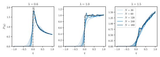
Figure 1: Numerical estimate for the overlap probability density function $\bar{P}(q)$ for a population of $M=50$ individuals averaged over $10^{5}$ generations. Several genome sizes are tested and depicted in different colors as explained in the legend, while the dashed curve corresponds to the theoretical probability distribution given by (18). As expected, if $\lambda<1$ mutations are likely and the overlap concentrates on values $q\approx 0$, if $\lambda>1$ mutations are rare and the overlap concentrates on values $q\approx 1$, while if $\lambda=1$ the probability distribution becomes uniform.

2.1.1 Exponential decay of correlations for efficient sampling

If we let the system evolve for a time $t\gg 1$, the last generation will be made up of individuals with a unique common ancestor with probability one in the asymptotic limit DP1 , hence it is possible to find an expression for the decay of genome-correlations between individuals at a given time and their common ancestor, as a function of time. Let us start evaluating the expectation value of the overlap between a parent $S^{G(a)}(t)$ and the corresponding offspring at $t+1$:

$$q_{\Delta t=1} = \mathbb{E}_{1}[\frac{\boldsymbol{S}^{G(a)}(t)\cdot\boldsymbol{S}^{a}(t+1)}{N}]=\frac{1}{N}\sum_{i=1}^{N}\mathbb{E}_{1}[S_{i}^{G(a)}(t)S_{i}^{a}(t+1)]$$ (21)

$$= \frac{1}{N}\sum_{i=1}^{N}\{1-2\mathbb{P}_{1}[S_{i}^{a}(t+1)=-S_{i}^{G(a)}(t)]\}$$ (22)

$$= 1-2\mathbb{P}_{1}[S_{i}^{a}(t+1)=-S_{i}^{G(a)}(t)]=e^{-2\mu},$$ (23)

where in the last line we exploited the fact that loci are independent. We can demonstrate that the expectation value of the overlap between a parent and the corresponding offspring at $t+\Delta t$ is

$$q_{\Delta t}=\mathbb{E}_{\Delta t}[\frac{S^{G^{\Delta t}(a)}(t)\cdot S^{a}(t+\Delta t)}{N}]=e^{-2\mu\Delta t},$$ (24)

where the average $\mathbb{E}_{\Delta t}$ is performed over the distribution $\mathbb{P}_{\Delta t}$ which generalizes (14). We prove this by induction: first we observe that $q_{\Delta t=1}=e^{-2\mu}$ is true, next we assume that $q_{\Delta t}=e^{-2\mu\Delta t}$ is true for any $\Delta t$ and we check that this is sufficient to ensure that also $q_{\Delta t+1}=e^{-2\mu(\Delta t+1)}$ is true. In the following, in order to lighten the notation, we shall we set $t=0$ without loss of generality and we shall drop the superscript labelling the individual without any loss of information: the individual we are referring to is $a$ or its ancestor at the generation specified by time dependence of $\boldsymbol{S}$.

Let use observe that $q_{\Delta t}$ can be written as

$$q_{\Delta t}=\frac{1}{N}\sum_{i=1}\{1-2\mathbb{P}_{\Delta t}[S_{i}(\Delta t)=-S_{i}(0)]\}$$ (25)

and, analogously, $q_{\Delta t+1}$ can be written as

$$q_{\Delta t+1}=\frac{1}{N}\sum_{i=1}\left\{1-2\mathbb{P}_{\Delta t+1}[S_{i}(\Delta t+1)=-S_{i}(0)]\right\}.$$ (26)

By the law of total probability we can write

$$\mathbb{P}_{\Delta t+1}[S_{i}(\Delta t+1) = -S_{i}(0)]=\mathbb{P}_{\Delta t}[S_{i}(\Delta t)=S_{i}(0)]\leavevmode\nobreak\ \mathbb{P}_{1}[S_{i}(\Delta t+1)=-S_{i}(\Delta t)]$$ (27)

$$+ \mathbb{P}_{\Delta t}[S_{i}(\Delta t)=-S_{i}(0)]\mathbb{P}_{1}[S_{i}(\Delta t+1)=S_{i}(\Delta t)].$$

Recalling that

$$\mathbb{P}_{1}[S_{i}(\Delta t+1)=-S_{i}(\Delta t)]=\frac{1-e^{-2\mu}}{2}$$ (28)

we reach

$$\mathbb{P}_{\Delta t+1}[S_{i}(\Delta t+1)=-S_{i}(0)]=\frac{1-e^{-2\mu}}{2}+e^{-2\mu}\mathbb{P}_{\Delta t}[S_{i}(\Delta t)=-S_{i}(0)].$$ (29)

By direct substitution of the last equation into (26) we get

$$q_{\Delta t+1}=\frac{e^{-2\mu}}{N}\sum_{i=1}\left\{1-2\mathbb{P}_{\Delta t}[S_{i}(\Delta t)=-S_{i}(0)]\right\}.$$ (30)

and, recalling the definition of $q_{\Delta t}$ given in (25), the last equation gets

$$q_{\Delta t+1}=\frac{e^{-2\mu}}{N}\sum_{i=1}\left[1-2\mathbb{P}_{\Delta t}(S_{i}(\Delta t)=-S_{i}(0))\right]=e^{-2\mu}q_{\Delta t}=e^{-2\mu(\Delta t+1)}.$$ (31)

In figure 2, the exponential decay of the overlap between the ancestor and its offsprings as a function of time is shown along with the related family tree.

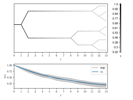
Figure 2: Upper panel: number of individuals generated by the ancestor as a function of the generation; in this particular evolution, all the individuals present at time $t=13$ turn out to stem from the same common ancestor and other branches that have not survived are omitted in this plot. The colormap highlights the overlap between the various individuals and the ancestor. Lower panel: time decay of the overlap between the ancestor and its offsprings; the numerical estimate (solid line) is consistent with the theoretical estimate $e^{-2\mu t}$ (dashed line); the shadow represents three standard deviations evaluated by repeating the process 100 times.

2.1.2 A new class of ultrametric identities

As stressed in Sec. 2.1, in the OPM the genome overlap is non self-averaging and $\overline{\langle q^{2}\rangle}-\overline{\langle q\rangle}^{2}\neq 0$. However, following spin-glass theory, one may wonder whether other kinds of relation hold among overlap momenta. As recalled in Sec. 2, in the SK and many variations of its, the Ghirlanda-Guerra and Aizenman-Contucci identities are preserved even under replica-symmetry-breaking. Here, to inspect the validity of these identities we study numerically the following quantities

$$\varepsilon_{\textrm{GG}}=\overline{\langle q_{12}^{4}\rangle}-2\overline{\langle(q_{12}q_{13})^{2}\rangle}+\mkern 1.5mu\overline{\mkern-1.5mu\langle q_{12}^{2}\rangle^{2}\mkern-1.5mu}\mkern 1.5mu$$ (32)

$$\varepsilon_{\textrm{AC}}=\mkern 1.5mu\overline{\mkern-1.5mu\langle q_{12}^{4}\rangle\mkern-1.5mu}\mkern 1.5mu-4\mkern 1.5mu\overline{\mkern-1.5mu\langle(q_{12}q_{13})^{2}\rangle\mkern-1.5mu}\mkern 1.5mu+3\mkern 1.5mu\overline{\mkern-1.5mu\langle q_{12}^{2}q_{34}^{2}\rangle\mkern-1.5mu}\mkern 1.5mu$$ (33)

$$\varepsilon_{\textrm{SA}}=\overline{\langle q_{12}^{4}\rangle}-\overline{\langle q_{12}^{2}\rangle^{2}},$$ (34)

where $\varepsilon_{\textrm{GG},\textrm{AC},\textrm{SA}}$ are interpreted as a measure of possible violation. Remarkably, since our inspection is only based on numerics, at finite population size and along a finite time span, in order to verify if non-null values of $\varepsilon_{\textrm{GG},\textrm{AC},\textrm{SA}}$ are intrinsic or, rather, stem from finite-size effects, we will perform a finite-size-scaling: if the extent of $\varepsilon$ is non-decreasing by increasing the system size, we will have a signature for the breakdown of the related identity.

Beyond these quantities, we can inspect the time-averaged joint probability density $\bar{P}(q_{12},q_{23},q_{13})$ of the overlaps $q$, in the infinite genome limit $N\to\infty$, that is known DP1 and reads as,

$$\begin{cases}\bar{P}(q_{12},q_{23},q_{13})=\frac{\lambda^{2}}{2}\theta(q_{23}-q_{12})\delta(q_{12}-q_{13})q_{12}^{\lambda-1}q_{23}^{2\lambda-1}+\text{Perm}(1,2,3)&q_{12},q_{13},q_{23}\in(0,1]\\ 0&\text{otherwise}\end{cases}$$ (35)

looking for possible relations among overlap momenta. In particular, we find that in the thermodynamic limit $N\to\infty$

$$\overline{\left\langle q_{12}^{K}\right\rangle}=\frac{\overline{\left\langle q_{12}\right\rangle}}{K+\overline{\left\langle q_{12}\right\rangle}(1-K)}=\frac{\lambda}{\lambda+K},\leavevmode\nobreak\ \forall K\in\mathbb{N},$$ (36)

which generalizes (19) and, by a direct calculation, we also find

$$\overline{\left\langle q_{12}^{\alpha}q_{13}^{\alpha}\right\rangle}=\frac{\lambda^{2}\left(5\alpha^{2}+8\alpha\lambda+3\lambda^{2}\right)}{(\alpha+\lambda)^{2}(2\alpha+\lambda)(2\alpha+3\lambda)},\leavevmode\nobreak\ \forall\alpha\in\mathbb{R}^{+}.$$ (37)

Now, by merging (36) and (37), we obtain the following relation, that plays as a new generator of overlap constraints for this model

$$\overline{\langle q_{12}^{2\alpha}\rangle}+\beta\overline{\langle q_{12}^{\alpha}q_{13}^{\alpha}\rangle}-(1+\beta)\frac{\overline{\langle q_{12}^{\alpha}\rangle}\,\overline{\langle q_{12}^{2\alpha}\rangle}\,\overline{\langle q_{12}^{2\alpha/3}\rangle}}{\overline{\langle q_{12}^{\frac{\alpha}{6}\left(5+\sqrt{\frac{25\beta+1}{\beta+1}}\right)}\rangle}\,\overline{\langle q_{12}^{\frac{\alpha}{6}\left(5-\sqrt{\frac{25\beta+1}{\beta+1}}\right)}\rangle}}=0.$$ (38)

Indeed, the above equation constitutes an infinite family of relations which hold for the OPM. In particular, due to the non-integrability of the overlap momenta with negative power, we must have $\beta\geq-1/25,\alpha\geq 0$ which fulfils the condition $5-\sqrt{\frac{25\beta+1}{\beta+1}}\geq 0$ ensuring that the moments of the overlap are well defined.
As an example, if we set $\alpha=2$ and $\beta=1/7$ in equation (38) we get

$$\overline{\langle q_{12}^{4}\rangle}+\frac{1}{7}\overline{\langle q_{12}^{2}q_{13}^{2}\rangle}-\frac{8}{7}\frac{\overline{\langle q_{12}^{2}\rangle}\,\overline{\langle q_{12}^{4}\rangle}\overline{\langle q_{12}^{4/3}\rangle}}{\overline{\langle q_{12}^{7/3}\rangle}\overline{\langle q_{12}\rangle}}=:\varepsilon_{1},$$ (39)

then, if we set $\alpha=2$ and $\beta=1/2$ in equation (38), we get

$$\overline{\langle q_{12}^{4}\rangle}+\frac{1}{2}\overline{\langle q_{12}^{2}q_{13}^{2}\rangle}-\frac{3}{2}\frac{\overline{\langle q_{12}^{2}\rangle}\,\overline{\langle q_{12}^{4}\rangle}\overline{\langle q_{12}^{4/3}\rangle}}{\overline{\langle q_{12}^{8/3}\rangle}\overline{\langle q_{12}^{\frac{2}{3}}\rangle}}=:\varepsilon_{2}$$ (40)

where we introduced $\varepsilon_{1}$ and $\varepsilon_{2}$ to measure possible failures of these relations. As shown in figure 3, both $\varepsilon_{1}$ and $\varepsilon_{1}$ are numerically found to vanish for the OPM. However, we stress that equations (39) and (40) are just two examples of equalities since there is an infinite family of relationships which are satisfied by the OPM and that can be obtained by varying $\alpha\in[0,+\infty)$ and $\beta\in[-1/25,+\infty)$ in equation (38). In Figure 3 we also show numerical evidence that self-averaging is broken (as expected by construction) and that nor the Ghirlanda-Guerra identities neither the Aizenman-Contucci polynomials seem to hold.

Figure 3: Errors measured for the various ultrametric identities as a function of the mean overlap for the OPM and for different values of $M$; the process average is taken over a run of $10^{2}\times M$ generations. Note that, as $M$ (and the time span, accordingly) grows, the error on self-averaging ($\varepsilon_{\textrm{SA}}$), on Ghirlanda-Guerra identities ($\varepsilon_{\textrm{GG}}$) and on Aizenman-Contucci polynomials ($\varepsilon_{\textrm{AC}}$) does not decrease, while the errors $\varepsilon_{1},\ \varepsilon_{2}$ are robustly vanishing.

2.2 The Homogeneous Population Model (HPM)

Serva and Peliti Peliti2 investigated a natural extension of the OPM, namely a two-parents model where parents can mate regardless their genome proximity; as a result of this feature, the long-time limit population is homogeneous (whence the name given to model) and, consequently, the model exhibits replica-symmetry in such a way that all the ultrametric constraints become trivial identities.

Figure 4: Distribution of the overlap $P(q,t)$ of the HPM at $\lambda=1.0$ and for different values of $M$ as shown in the legend. As $M$ is made larger and larger $P(q,t)$ gets monomodal and peaked at $\langle q\rangle_{t}=1/2$, thus highlighting a replica symmetric behavior of the specie evolution in the HPM.

In the HPM, at each generation $t$, each individual $a$ has two distinct parents $G_{1}(a)$ and $G_{2}(a)$ chosen at random from the previous generation. Each spin $S_{i}^{a}$ is inherited from either $G_{1}(a)$ or $G_{2}(a)$ with equal probability, with the same probability of faithful copy or mutation as in equation (14). In the OPM model if the overlap between the parents $G(a)$ and $G(b)$ of two individuals, $a$ and $b$, is $q_{G(a)G(b)}$ then the expectation value of the overlap of $a$ and $b$ is

$$q_{ab}=e^{-4\mu}q_{G(a)G(b)}.$$ (41)

If $N$ is infinite this becomes a deterministic rule for updating the overlap matrix. There is an equivalent rule for updating the overlap matrix for the HPM in the limit $N\to\infty$. The pair of spins $S_{i}^{a}S_{i}^{b}$ is inherited from one of the four combinations of parents of the two individuals with equal probability, therefore

$$q_{ab}=\frac{e^{-4\mu}}{4}(q_{G_{1}(a)G_{1}(b)}+q_{G_{2}(a)G_{1}(b)}+q_{G_{1}(a)G_{2}(b)}+q_{G_{2}(a)G_{2}(b)})$$ (42)

with $q_{aa}=1$ always. It can be proven that the variance of $\langle q\rangle_{t}$ vanishes in the limit $M\to\infty$, thus $\langle q\rangle_{t}$ is self-averaging in the HPM, in particular $\lim_{M\to\infty}\mkern 1.5mu\overline{\mkern-1.5mu\langle q\rangle\mkern-1.5mu}\mkern 1.5mu=\frac{\lambda}{1+\lambda}$.

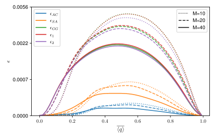
Figure 5: Errors measured for the various ultrametric identities as a function of the mean overlap for the HPM and for different values of $M$; the process average is taken over a run of $10^{2}\times M$ generations Note that, as $M$ grows, all the errors depicted tend to approach the horizontal axes as expected since the overlap is self-averaging in this model.

Figure 4 shows results about the overlap distribution for long simulations of the HPM model with $\lambda=1$ and, accordingly, $\lim_{M\to\infty}\overline{\langle q\rangle}=1/2$: the various rows show the overlap distribution $P(q,t)$ sampled at different times and by inspecting its variance as a function of $M$ it can be shown that it scales as $1/M$ hence it is expected to disappear for large population size $M$ such that $P(q,t)$ gets concentrated around $q=1/2$, showing that self-averaging of the overlap is respected hence proving that the model behaves in a replica symmetric manner. Consistently, in figure 5 we show that the errors on the ultrametric identities approaches zero as $M$ is made larger and larger.

Figure 6: Distribution of the overlap $P(q,t)$ of the SFM for $\lambda=1.0,q_{min}=0.65,M=2000$. Note that, at difference w.r.t. the previous replica-symmetric HPM, here there actually are new specie formation and extinction as the presence of several peaks in the $P(q,t)$ evidences. Further, beyond the big one on the left (that is exponentially collapsing toward zero as time goes on), the erratic presence of these small peaks confirms that the SFM gives rise to an evolutive scenario strongly resembling the paining by replica-symmetry-breaking of the low temperature spin glasses.

2.3 The Specie Formation Model (SFM)

The SFM introduced by Higgs and Derrida Derrida2 ; Derrida3 is nothing but the two-parents model of Serva and Peliti with a threshold for mating $q_{min}$. Specifically, it is defined in the same ways as the HPM earlier, except that the first parent $G_{1}(a)$ of individual $a$ is chosen randomly from the previous generation whereas the second $G_{2}(a)$ is chosen only from those individuals having an overlap $q_{G_{1}(a)G_{2}(a)}$ greater than a cutoff value $q_{min}$. In the absence of a cutoff, thus in the case of HPM, there is a natural mean value of the overlap $\mkern 1.5mu\overline{\mkern-1.5mu\langle q\rangle\mkern-1.5mu}\mkern 1.5mu=\lambda/(1+\lambda)$, in such a way that, if the SFM $q_{min}>\lambda/(1+\lambda)$, the system is highly perturbed by the introduction of the threshold and it can never reach its natural equilibrium state: $\pi\acute{\alpha}\nu\tau\alpha\;\grave{\rho}\varepsilon\widetilde{\iota}$ as in the low temperature regime of spin glasses.
A corroboration of this picture appears in figure 6 where we show the distribution of the overlap $P(q,t)$ at different times: the peaks appearing above the threshold $q_{min}>0.65$ correspond to the overlaps of the new species that have formed (and their disappearance to their extinction) while the large peak below the threshold exponentially collapses toward zero (since such values of the overlap are lower than $q_{min}$ no interbreeding is possibile between them and, consequently, the peak must be vanishing).

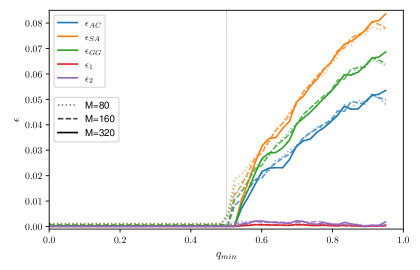
Figure 7: Errors measured for the various ultrametric identities as a function of the mating threshold $q_{min}$ for the SFM and for different values of $M$; the process average is taken over a run of $10^{2}\times M$ generations. At the numerical level, the new set of identities keep holding also for the SFM, while all the other constraints seem to be violated.

2.3.1 Numerical inspection of ultrametric constraint’s violation in the SFM

We now study numerically the validity of all the ultrametric identities as well as of the self-averaging, by measuring the related errors $\varepsilon$. Specifically, we set $\lambda=1$ in such a way that the expected value in the HPM is $\overline{\langle q\rangle}=\frac{1}{2}$ and we vary $q_{min}\in[0,1]$. We simulate the evolution over a population of size $M$ and a time span $10^{2}\times M$, and we collect data for $\varepsilon_{1},\ \varepsilon_{2},\ \varepsilon_{\textrm{GG}},\ \varepsilon_{\textrm{SA}},\ \varepsilon_{\textrm{AC}}$ that are plotted in Figure 7 versus $q_{min}$. As expected, when $q_{min}<\frac{1}{2}$, the threshold does not involve significant effects with respect to the HPM and a replica-symmetric scenario is recovered with errors $\varepsilon$ close to zero. Conversely, the region $q_{min}>\frac{1}{2}$ is non-trivial and there emerge differences between the errors. As for the classical identities and for the variance, the related errors ($\varepsilon_{\textrm{SA},\textrm{GG},\textrm{AC}}$) are non-vanishing, and their values grows with $q_{min}$ without any robust trend with respect to the size $M$; as for the new identities, the related errors ($\varepsilon_{1,2}$) remain close to zero.

2.3.2 Numerical inspection of ultrametric constraint’s violation in biological and artificial human genomes

In this Section we look for any evidence of the relations discussed before in actual genomic datasets. To this aim we tested all the ultrametric identities and the self-averaging property on the biological genome collected by The 1000 Genomes Project Consortium Dati1 and on artificial genomes generated by two neural neworks (a Generativa Adversarial network and a Restricted Boltzmann machine) Dati2 ; notably, the latter have already proved to reproduce correctly allele frequencies, linkage disquilibrium, pairwise haplotype distances and population structure.

As in Dati2 ; Dati3 , we consider a population of $M=2504$ individuals ($\sim 5\cdot 10^{3}$ haplotypes) spanning $N=805$ Single Nucleotide Polymorphism (SNPs) from Dati1 , which reflect a high proportion of the population structure present in the whole dataset Dati2 ; 25 . The various fluctuation relations are evaluated by splitting the dataset of $M$ individuals into $\sqrt{M}$ groups: the population average $\langle\>\cdot\>\rangle$ is carried out by identifying distinct replica indices with distinct individuals within the same group. In contrast, the process average $\overline{\>\cdot\>}$ is carried out by performing an arithmetic mean over the different evaluations of each group. Regarding the finite size scaling in $N$ it has been carried out by selecting a common subset of size $N$ of the genome variable $(-1,+1)$ for each individual.

Results are collected in Figure 8 and show that also in these structured datasets the new set of identities is better respected w.r.t. the classical ones (despite the violation of the latter is minimal in these settings).

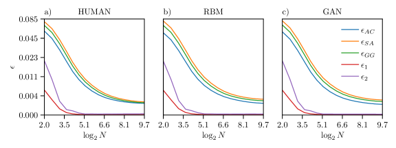
Figure 8: Finite-size-scaling on genome length testing the various ultrametric identities for the real human genome (HUMAN, taken from Dati1 ) and two artificial genomes (taken from Dati2 ) generated rispectively with a Generative Adversarial Network (GAN) and a Restricted Botlzmann machine (RBM). In these settings still our new family of identities seems to be respected, while mild violations of the others persist (despite their violation is minimal, i.e. $\varepsilon_{\textrm{AC}}\sim\varepsilon_{\textrm{GG}}\sim O(10^{-3})$).

3 Conclusions

The non-self-averaging behavior of the order parameter in spin-glass models is a peculiar, intensively-studied feature which can be described in terms of a set of relations connecting the fluctuations of the order parameter. Driven by strong analogies between Natural Evolution and statistical mechanics of disordered systems, we investigated the validity of these ultrametric relations and the existence of other kinds of relations focusing on three stochastic models of evolving populations in flat landscapes. These models are the fairly standard ones in the Literature on Natural Evolution without selective pressure, that is (i) the One Parent Model (OPM) – where reproduction is asexual and the distribution of genetic distances lacks self-averaging – (ii) the Homogeneous Population Model (HPM) – where reproduction is sexual and with random mating (i.e., regardless the genetic distance) and thus results in a replica symmetric picture where the genetic distance between pairs of individuals has vanishing fluctuations in the thermodynamic lmiit (hence the adjective homogeneous in the model’s name) – and (iii) the Specie Formation model (SFM) where reproduction is still sexual but with a threshold on the required similarity among mating genomes before duplication. The latter represents the most interesting case as it is the closest to biology and it spontaneously gives rise to a complex dynamics reaching a steady state with new species that are continuously and spontaneously generated and suppressed during the evolutionary process. Further, while in the first model the evolutionary tree is assumed and it is related to single descendants from common ancestors, in the latter the evolutionary tree emerges and it works at the level of species rather than single elements.
Focusing on fluctuations in the genetic distances between individuals, as far as the OPM is concerned, after checking that self-averaging is absent in this model statistics, we have shown by a finite-size-scaling argument that nor the Ghirlanda-Guerra identities neither the Aizenman-Contucci polynomials are respected. On the other hand, we were able to prove a new class of identities that are indeed respected also in our finite-size numerical checks. For HPM, as it is replica symmetric, all these constraints are equally guarantee to converge to zero in the asymptotic limit but they do not convey actual information. Then, dealing with the SFM, our identities continue to hold, being only mildly affected by finite-size effects.

As a final test we focused on human gemomes: we considered the real biological dataset taken from the 1000 genome project consortium and two synthetic datasets on artificial genomes generated by neural networks and, for all these three cases the scenario depicted by the SFM seems to be confirmed here as well: the new set of ultrametric identities is sharply respected while mild violations affect both Ghirlanda-Guerra identities as well as Aizenman-Contucci polynomials.

As models of Natural Evolution under selective pressure, namely Darwinian Evolution, are known to display standard Ghirlanda-Guerra fluctuations (from the Franz-Peliti-Sellitto model, i.e., the $P\to\infty$ limit of the Kauffman-Levin P-spin-glass model, or the REM in a spin-glass jargon to the equal-trap model analyzed by Leuthäusser and Tarazona the Hopfield model in spin glass jargon), a similar analysis to the present one should be conducted also in these settings to better infer the role covered by Natural Selection (beyond random mutation) in shaping evolutionary taxonomies because, at present, these new findings seem to be in better agreement with Kimura Theory of Neutral Evolution: we plan to report soon on this topic.

References

- [1] G. Parisi, A sequence of approximated solutions to the SK model for spin glasses, J. Phys. A 13.4: L115, (1980).
- [2] G. Parisi, The order parameter for spin glasses: a function on the interval 0-1, J. Phys. A 13.3: 1101, (1980).
- [3] J. Van Mourik, A. C. C. Coolen, Cluster derivation of Parisi’s RSB solution for disordered systems, J. Phys. A 34.10:L111, (2001).
- [4] D.J. Amit, Modeling brain function: the world of attractor neural networks, Cambridge University press, (1989).
- [5] G. Tkacik, et al., The simplest maximum entropy model for collective behavior in a neural network, J. Stat. Mech. 2013.03: P03011, (2013).
- [6] H. Huang, Statistical mechanics of neural networks, Springer Press, (2021).
- [7] A. Braunstein, et al., Inference algorithms for gene networks: a statistical mechanics analysis, J. Stat. Mech. 2008.12: P12001, (2008).
- [8] G. Torrisi, R. Kuehn, A. Annibale, Percolation on the gene regulatory network, J. Stat.l Mech. 2020.8: 083501, (2020).
- [9] T. Mora, et al., Maximum entropy models for antibody diversity, Proc. Natl. Acad. Sci. 107.12:5405-5410, (2010).
- [10] E. Agliari, et al., Anergy in self-directed B lymphocytes: a statistical mechanics perspective, J. Theor. Biol. 375:21-31, (2015).
- [11] A. Murugan, et al., Statistical inference of the generation probability of T-cell receptors from sequence repertoires, Proc. Natl. Acad. Sci. 109.40:16161-16166, (2012).
- [12] W. Bialek, et al., Statistical mechanics for natural flocks of birds, Proc. Natl. Acad. Sci. USA 109.13: 4786-4791, (2012).
- [13] R.V. Solé, J. Bascompte, Self-Organization in Complex Ecosystems, Princeton Univ. Press (2006).
- [14] R.V. Solé, S.C. Manrubia, M. Benton, S. Kauffman, P. Bak, Criticality and scaling in evolutionary ecology, Trends in Ecol. Evol. 14(4):156-160, (1999).
- [15] A. Barra, P. Contucci, R. Sandell, C. Vernia, An analysis of a large dataset on immigrant integration in Spain: the statistical mechanics perspective on social action, Nature Sci. Rep. 4(1), 1-7 (2014).
- [16] S.N. Durlauf, How can statistical mechanics contribute to social science?, Proc. Natl. Acad. Sci. USA 96.19:10582-10584, (1999).
- [17] A.C.C. Coolen, The mathematical theory of minority games: statistical mechanics of interacting agents, Oxford Univ. Press (2005).
- [18] M. Cristelli, et al., Measuring the intangibles: a metrics for the economic complexity of countries and products, PloS one 8.8: e70726, (2013).
- [19] M. Mézard, G. Parisi, R. Zecchina, Analytic and algorithmic solution of random satisfiability problems, Science 297.5582: 812-815, (2002).
- [20] M. Mézard, A. Montanari, Information, physics, and computation, Oxford Univ. Press (2009).
- [21] S. Kauffman, S. Levin, Towards a general theory of adaptive walks on rugged landscapes, J. Theor. Biol. 128.1:11-45, (1987).
- [22] S. Franz, L. Peliti, M. Sellitto, An evolutionary version of the random energy model, J. Phys. A 26.23: L1195, (1993).
- [23] P. Tarazona, Error thresholds for molecular quasispecies as phase transitions: from simple landscapes to spin-glass models, Phys. Rev. A 45.8:6038, (1992).
- [24] B. Derrida, L. Peliti, Evolution in a flat fitness landscape, Bull. Math. Biol. 53.3:355-382, (1991).
- [25] M. Eigen, Viral quasispecies, Sci. Amer. 269.1: 42-49, (1993).
- [26] M. Nowak, R.M. May, Virus dynamics: mathematical principles of immunology and virology, Oxford University Press, UK, (2000).
- [27] E. Agliari, A. Barra, R. Burioni, A. Di Biasio, G. Uguzzoni, Collective Behaviours: from biochemical kinetics to electronic circuits, Sci. Rep. 3, 3458, (2013).
- [28] E. Agliari, M. Altavilla, A. Barra, L. Dello Schiavo, E. Katz, Notes on stochastic (bio)-logical gates: computing with allosteric cooperativity, Sci. Rep. 5, 9415, (2015).
- [29] E. Agliari, A. Barra, L. Dello Schiavo, A. Moro, Complete integrability of information processing by biochemical reactions, Sci. Rep. 6, 36314 (2016).
- [30] I. Leuthäusser, Statistical mechanics of Eigen’s evolution model, J. Stat. Phys. 48:343-360, (1987).
- [31] P. Higgs, B. Derrida, Stochastic models for species formation in evolving populations, J. Phys. A 24.17: L985, (1991).
- [32] P. Higgs, B. Derrida, Genetic distance and species formation in evolving populations, J. Mol. Evol. 35.5:454-465, (1992).
- [33] M. Serva, L. Peliti, A statistical model of an evolving population with sexual reproduction, J. Phys. A 24.13: L705, (1991).
- [34] L. Peliti, Introduction to the statistical theory of Darwinian evolution, arXiv preprint cond-mat/9712027, (1997).
- [35] E. Svensson, R. Calsbeek (eds.), The adaptive landscape in evolutionary biology, Oxford Univ. Press, Oxford, (2012).
- [36] M. Kimura, The neutral theory of molecular evolution, Cambridge University Press, (1983).
- [37] S.A. Frank, M. Slatkin, Fisher’s fundamental theorem of natural selection, Trends in Ecol. Evol. 7.3:92-95, (1992).
- [38] M. Aizenman, P. Contucci, On the stability of the quenched state in mean-field spin-glass models, J. Stat. Phys. 92.5:765-783, (1998).
- [39] A. Barra, Irreducible free energy expansion and overlaps locking in mean field spin glasses, J. Stat. Phys. 123.3:601-614, (2006).
- [40] P. Contucci, C. Giardiná, The Ghirlanda-Guerra identities, arXiv preprint math-ph/0505055 (2005).
- [41] S. Ghirlanda, F. Guerra, General properties of overlap probability distributions in disordered spin systems. Towards Parisi ultrametricity, J. Phys. A 31.46, 9149, (1998).
- [42] L. Viana, A.J. Bray, Phase diagrams for dilute spin glasses, J. Phys. C 18.15:3037, (1985).
- [43] A. Barra, L. De Sanctis, Stability properties and probability distributions of multi-overlaps in dilute spin glasses, JSTAT 2007.08:P08025, (2007).
- [44] L. De Sanctis, S. Franz, Self-averaging identities for random spin systems, Spin Glasses: Statics and Dynamics: Summer School, Paris 2007.
- [45] S. Franz, M. Leone, Replica bounds for optimization problems and diluted spin systems, J. Stat. Phys. 111:535-564, (2003).
- [46] R. Burioni, et al., Notes on the p-spin glass studied via Hamilton-Jacobi and smooth-cavity techniques, J. Math. Phys. 53.6: 063304, (2012).
- [47] P. Contucci, C. Giardiná, Perspectives on spin glasses, Cambridge Univ. Press, (2013).
- [48] D. Panchenko, The Ghirlanda Guerra identities for mixed p-spin model, Comp. Ren. Math. 348.3-4: 189-192, (2010).
- [49] M. Aizenman, M. R. Sims, S. L. Starr, Extended variational principle for the Sherrington-Kirkpatrick spin-glass model, Physical Review B 68.21 (2003): 214403.
- [50] W.K. Chen, The Aizenman-Sims-Starr scheme and Parisi formula for mixed p-spin spherical models Electr. Journ. Prob. 18:94, 1-14, (2013).
- [51] P. Sollich, A. Barra, Spin glass polynomial identities from entropic constraints, J. Phys. A 45.48:485001, (2012).
- [52] A. Barra, F. Guerra, Constraints for the order parameters in analogical neural networks, arXiv preprint arXiv:0911.3113, (2009).
- [53] A. Bovier, I. Kurkova, Derrida’s Generalized Random Energy models 2: models with continuous hierarchies, Ann. H.P. Prob. Stat. 40.4, (2004).
- [54] A. Bovier, I. Kurkova, Derrida’s generalized random energy models 4: continuous state branching and coalescents, No. MP-ARC-2003-247. WIAS, (2003).
- [55] P. Contucci, C. Giardiná, Spin-glass stochastic stability: a rigorous proof, Ann. H. Poincare 6, 5, (2005).
- [56] P. Contucci, C. Giardiná, C. Giberti, Interaction-flip identities in spin glasses, J. Stat. Phys. 135.5:1181-1203, (2009).
- [57] S. Chatterjee, The Ghirlanda-Guerra identities without averaging, arXiv preprint arXiv:0911.4520, (2009).
- [58] L.P. Arguin, Competing particle systems and the Ghirlanda-Guerra identities arXiv: 2101-2117, (2018).
- [59] Y.T. Chen, Universality of Ghirlanda Guerra identities and spin distributions in mixed p-spin models , Ann. H.P. Prob. Stat. 55: 528-550, (2019).
- [60] M. Talagrand, The Ghirlanda-Guerra Identities, Mean Field Models for Spin Glasses II:287-311, (2011).
- [61] D. Panchenko, A connection between the Ghirlanda Guerra identities and ultrametricity, Ann. Prob. 38.1:327-347, (2010).
- [62] D. Panchenko, Ghirldanda Guerra identities and ultrametricity: an elementary proof in the discrete case, Compt. Ren. Math. 349.13-14:813-816, (2011).
- [63] D. Panchenko, The Parisi ultrametricity conjecture, Ann. Math. 383-393, (2013).
- [64] D. Sherrington, S. Kirkpatrick, Solvable model of a spin-glass, Phys. Rev. Lett. 35.26: 1792, (1975).
- [65] V.S. Dotsenko, Physics of the spin-glass state, Physics-Uspekhi 36.6:455, (1993).
- [66] F. Guerra, Broken replica symmetry bounds in the mean field spin glass model, Comm. Math. Phys. 233: 1-12, (2003).
- [67] M. Talagrand, The parisi formula, Ann. Math. 221-263, (2006).
- [68] P. Contucci, C. Giardiná, C. Giberti, G. Parisi, C. Vernia, Ultrametricity in the Edwards-Anderson model, Phys. Rev. Lett. 99(5), 057206, (2007).
- [69] A. Barra, L. De Sanctis, Overlap fluctuations from the Boltzmann random overlap structure, J. Math. Phys. 47.10:103305, (2006).
- [70] E. Gardner, Spin glasses with p-spin interactions, Nucl. Phys. B 257: 747-765, (1985).
- [71] B. Derrida, Random-energy model: limit of a family of disordered models, Phys. Rev. Lett. 45, 79-82, (1980.
- [72] L. Peliti, Quasispecies evolution in general mean-field landscapes, Europhys. Lett. 57.5: 745, (2002).
- [73] The 1000 Genomes Project Consortium, A global reference for human genetic variation, Nature 526, 68-74, (2015).
- [74] B. Yelmen, et al., Creating artificial human genomes using generative neural networks, PLoS Gen. 17(2):e1009303, (2021).
- [75] A. Decelle, L. Rosset, B. Seoane, Unsupervised hierarchical clustering using the learning dynamics of RBMs, arXiv:2302.01851v2, (2022).
- [76] V. Colonna, et al., Human genomic regions with exceptionally high levels of population differentiation identified from 911 whole-genome sequences, Genome Biol. 15:R88, (2014)