Depinning free of the elastic approximation

Abstract

We model the isotropic depinning transition of a domain-wall using a two dimensional Ginzburg-Landau scalar field instead of a directed elastic string in a random media. An exact algorithm accurately targets both the critical depinning field and the critical configuration for each sample. For random bond disorder of weak strength $\Delta$, the critical field scales as $\Delta^{4/3}$ in agreement with the predictions for the quenched Edwards-Wilkinson elastic model. However, critical configurations display overhangs beyond a characteristic length $l_{\tt 0}\sim\Delta^{-\alpha}$, with $\alpha\approx 2.2$, indicating a finite-size crossover. At the large scales, overhangs recover the orientational symmetry which is broken by directed elastic interfaces. We obtain quenched Edwards-Wilkinson exponents below $l_{\tt 0}$ and invasion percolation depinning exponents above $l_{\tt 0}$. A full picture of domain wall isotropic depinning in two dimensions is hence proposed.

In recent decades, significant progress has been made in understanding a paradigmatic example of out-of-equilibrium critical phenomena: the depinning transition of elastic interfaces in random media [1, 2, 3, 4]. Depinning is relevant in various extended physical systems, such as ferromagnetic [5] and ferroelectric [6, 7] driven domain walls (DWs), tensioned cracks in hard and soft matter [8, 9, 10], the displacement of contact lines of liquid menisci [11, 12, 13], or even stressed tectonic plates and earthquakes [14, 15]. The common basic phenomenology of the depinning transition is well-captured by the simple model of a driven overdamped elastic interface coupled to a quenched disordered energy landscape that tends to trap the interface in configurations in which the potential energy is locally minimized. Under the application of a uniform external driving force $f$ the energy potential tilts. The interface might move slightly, but if the amplitude of the driving force is below a well defined threshold $f_{c}$, it eventually pins and remains immobile. Instead, it sets into a steady-state motion, with an average velocity $v>0$, if the driving force is above $f_{c}$. Exactly at $f_{c}$, the interface accommodates in a critical depinning configuration, exhibiting interesting universal geometrical properties.

Most progress in the field has been made by approximating the interface as univalued and using smooth scalar displacement fields for its dynamics, modeling it with overdamped equations like the driven quenched-Edwards-Wilkinson (qEW) model. Through powerful analytical and numerical techniques, researchers have found that the depinning transition at $f_{c}$ is continuous, non-hysteretic, and occurs at a well-defined characteristic threshold force $f_{c}$ [16]. At $f_{c}$ the interface is marginally blocked, and the instability is described by a localized soft spot or eigenvector [17]. Just above the threshold, the mean velocity $v$ follows the depinning law $v\sim(f-f_{c})^{\beta}$, with $\beta$ being a non-trivial critical exponent [18]. A divergent correlation length $l\sim(f-f_{c})^{-\nu}$ and a divergent correlation time $\tau\sim l^{z}$ characterize the jerky motion as $f_{c}$ is approached from above. Below the length-scale $l$, the rough geometry of the interface becomes self-affine (SA), with the displacement field growing as $u\sim x^{\zeta}$ for length-scales $x$ below $l$. Hence $v\sim l^{\zeta-z}$ and $\beta=\nu(z-\zeta)$. Depinning critical exponents have been studied both analytically [19, 20] and numerically [21, 22, 23, 24, 25, 26, 27]. Different universality classes are determined by the dimension of the interface $d$, the range [28, 29, 30, 31, 32] or nature [33] of the elastic interactions, the anisotropic [34] or isotropic correlations of the pinning forces [35, 36], and by the presence of additional non-linear terms [37, 34, 38, 39, 40, 41, 42, 43]. If the so-called statistical tilt symmetry holds, only two exponents are needed to fully characterize the depinning universality class. At large velocities, the effect of disorder mimic thermal fluctuations, and $v\sim f$. For $f<f_{c}$, motion is only possible through thermal activation at a finite temperature $T$. Particularly, for $f\ll f_{c}$ and relatively small temperatures, the universal creep-law [44, 45, 46] $\ln v(f)\sim-f^{-\mu}/T$ holds, with $\mu$ being a critical exponent related to dimension and the roughness exponent of the SA interface at thermal equilibrium ($f=0$). Remarkably, in this ultra-slow creep regime, a depinning criticality emerges at large scales, as observed both in the steady-state geometry and in the spatio-temporal fluctuations [47, 48, 49, 50, 51]. Furthermore, several of these qEW predictions are quantitatively confirmed by experiments conducted on ultra-thin ferromagnetic films with perpendicular anisotropy [52, 5, 53, 54, 51, 55].

However, the success of the elastic theory conflicts with the observation that, in the same experimental systems, domain wall configurations often exhibit overhangs and pinch-off loops, which, in fact, challenge the assumptions of the elastic theory. The natural question that arises is: Why, then, does the theoretically minimalist approach of a purely elastic interface work so well?

It is a common experimental practice to focus the analysis in a region displaying a “well behaved” univalued DW segment far from the nucleation centers and “rare defects” to test the theory. However, it is not clear whether overhangs are generated solely by rare strong pinning centers or extrinsic defects, as suggested by Ferre et al. [5], or whether they are generated by intrinsic defects that act cooperatively. This type of intrinsic disorder is characterized by statistically uniform weak disorder with short-range correlations, as assumed in the elastic theory. In other words, overhangs, fingers, and bubbles might be part of the solution of the actual critical interface in weak disorder and not an issue to be avoided. Understanding why and to what extent the elastic theory applies is an important open question to gain a full understanding of the domain wall dynamics.

In this work, using a disordered scalar Ginzburg-Landau (GL) model [56, 57, 58, 59], which does not break isotropy, we free ourselves from the elastic approximation, allowing for plasticity and realistic deformations of the interface. With the help of an accurate algorithm, the critical fields and interface configurations can be solved at depinning for different realizations of the disorder. Our analysis ultimately provides a comprehensive picture of DW depinning in two-dimensional isotropic media with short-range correlated disorder. Critical configurations always display overhangs beyond a characteristic length $l_{\tt 0}$ that depends on the disorder strength $\Delta$, indicating a finite-size crossover. Below $l_{\tt 0}$, we obtain quenched Edwards-Wilkinson exponents, and above $l_{\tt 0}$, we observe invasion percolation depinning exponents.

It’s worth mentioning that other approaches to the isotropic depinning transition have been pursued. Numerical simulations of the random-field Ising model (RFIM) suggest that in two dimensions, the DW critical configurations at the depinning threshold should be either faceted or self-similar (SS), instead of the self-affine (SA) geometry predicted by the elastic theory [60, 61]. However, these simulations are unable to address the isotropic depinning transition in the relevant weak disorder case due to the coupling of their thin domain walls to the underlying periodic lattice [61], which breaks isotropy.

The paper is organized as follows: Sec.I introduces the model. Sec. II presents the algorithm that we developed to target the critical configurations at depinning. In Sec.III, we describe and discuss our numerical results: first, the critical field (Sec. III.1) and then the geometry of the critical configurations (Sec.III.2). In Sec. IV, we summarize our conclusions. The appendix contains further details of the numerical computations.

I Model

We consider the following time-dependent Ginzburg-Landau equation for a scalar order parameter field $\phi(x,y)$, describing approximately the zero-temperature evolution of the out of plane magnetization in a ferromagnetic film with perpendicular anisotropy [56, 57, 58, 59],

$$\gamma\partial_{t}\phi=c\nabla^{2}\phi+\epsilon_{0}[(1+r(x,y))\phi-\phi^{3}]+{h}.$$ (1)

Here, the elastic constant $c$, $\epsilon_{0}$ and the friction $\gamma$ are positive constants, $h$ is the constant and uniform magnetic field, and $r(x,y)$ is a quenched random bond disorder specified by

$$\overline{r(x,y)} = 0,$$

$$\overline{r(x^{\prime},y^{\prime})r(x,y)} = \frac{2}{3}\Delta^{2}\delta(x-x^{\prime})\delta(y-y^{\prime}),$$ (2)

We denoted $\overline{(...)}$ the average over disorder realizations and $\Delta$ the disorder strength. We are interested in the limit of small disorder where the ground state at zero field is ferromagnetic (i.e. either $\phi\approx 1$ or $\phi\approx-1$).

We prepare the system with a small positive domain, namely $\phi\approx 1$ for $y<y_{0}$ and $\phi=-1$ for $y>y_{0}$. After an initial transient at $h=0$ we observe a well defined domain wall of width $\delta\approx\sqrt{c/\epsilon_{0}}$ and surface tension (DW energy per unit length) $\sigma\approx\sqrt{c\epsilon_{0}}$. The location of the wall is defined as the level zero set of the magnetization, i.e. the set of points $(x^{*},y^{*})$ where $\phi(x^{*},y^{*})=0$. Upon the application of a magnetic field $h$ (that favors the positive $\phi$ phase) the domain wall would acquire a steady velocity $v(h)=mh$, with $m\approx\delta/\gamma$ the mobility of the wall; but in the presence of disorder, the velocity-field characteristics becomes non-linear and displays a depinning transition: above a threshold field $h_{\tt d}$ the DW slides at a finite velocity, while below it the wall gets trapped into one of many metastable states. This has been clearly observed and quantified even in these scalar GL models where interfaces are not forced to be univalued [56]. Our goal is to determine $h_{\tt d}$, and the last metastable state or critical configuration $\phi_{d}(x,y)$, as $h\to h_{\tt d}$ from below.

II Algorithm

Eq.(1) is discretized with a regular $L\times L$ grid with coordinates $(i,j)$.

$$\partial_{t}\phi_{i,j} = c[\phi_{i+1,j}+\phi_{i+1,j}+\phi_{i,j+1}+\phi_{i,j-1}-4\phi_{i,j}]$$ (3)

$$+ \epsilon_{0}[(1+r_{i,j})\phi_{i,j}-\phi_{i,j}^{3}]+{h}=0,$$

Here, $r_{i,j}$ are uncorrelated random numbers sampled from a uniform distribution in $[-\Delta,\Delta]$. Setting $0<\Delta<1$, the term proportional to $\epsilon_{0}$ in Eq.(3) admits always three zeros for $|\phi_{i,j}|<1$. We apply periodic boundary conditions in the $x$ direction $\phi_{i+L,j}=\phi_{i,j}$, but anti-periodic boundary conditions in the $y$ direction, $\phi_{i,L}=-\phi_{i,0}$ to ensure that the evolution affect a single domain wall.

Starting from an arbitrary initial configuration (typically with a flat interface), we evolve the scalar field $\phi_{i,j}$ according to the so-called “variant Monte Carlo” method [38, 24, 62]. An elementary move updates $\phi_{i,j}$ by replacing it to one of the roots of Eq.(3) with $\partial_{t}\phi_{i,j}=0$. Using the François Viète formula for the cubic equation we find at most three real roots. The root that we select is the closer to the initial position $\phi_{i,j}$. The elementary steps are repeated consistently over the sites $(i,j)$, until the (positive) mean velocity of the order parameter is smaller than a small cutoff $\epsilon=10^{-4}$, signaling the proximity to a metastable state.

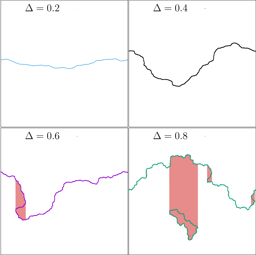
Figure 1: Typical critical configurations of the domain wall for different values of the disorder strength $\Delta$. System size is ${L=4096}$ (the aspect ratio is one). Red shaded regions highlight overhangs and/or pinch-off loops

This strategy relies on the Middleton theorems The “no-passing theorem” assures that the algorithm connects an arbitrary initial state with the critical configuration, whereas the “forward-moving theorem” justifies the approach of making only forward directed elementary moves [62]. This allows us to use the same technique developed in Refs. [38, 24, 62] for the elastic interface. The novelty of our implementation is that instead of applying it to the 1D DW displacement field, we apply it directly to the 2D order-parameter $\phi_{i,j}$. The order parameter is always univalued and bounded and has a convex elastic energy, though it can nucleate the multivalued critical DW we are more generally interested in. The algorithm proposed is, for a given accuracy, faster than the actual dynamics of Eq.(1); because elementary moves are not proportional to any numerical integration time-step, but instead controlled by a root finding method . We thus alleviate the critical-slowing down near all metastable states.

Furthermore, many of the computations involved in the implementation of the algorithm can be performed simultaneously, thus offering a valuable opportunity for an optimization via parallelization. These computations, such as elementary moves using the checkerboard decomposition, DW detection and other image processing like routines and reductions to obtain properties are accelerated using graphics processors. To apply the algorithm we discretize the two dimensional space and use finite differences to evaluate the derivatives. We consider square systems of size $L\times L$. Without loss of generality we choose $\epsilon_{0}=1$, $c=1$, $\gamma=1$, and for each disorder realization we drew $L\times L$ uncorrelated numbers $r(x,y)$ from a uniform distribution. The correlation length of the disorder $r_{\tt f}$ is thus of the order of the discretization itself and smaller than the DW width which then becomes the correlation length of the pinning force on DWs.

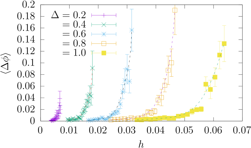
Figure 2: Magnetization jump per site $\langle\phi\rangle$ as a function of $h$, for different values of the disorder strength $\Delta$. Data correspond to averages over 50 samples, $L=256$. Dashed-lines are guides to the eye.

We build a sequence of metastable states as a function of $h$ until we localize $h_{\tt d}$, above which no metastable state can be found in the sample. Typical critical configurations for different values of $\Delta$ are shown in Fig.1. Overhangs can be clearly identified in the shaded-areas (defined as the regions where the interface adopts more than one value in the advancement direction) and they are more frequent for large disorder. Interestingly, for the largest disorder we can also see isolated pinned pinch-off loops signaling domains that were not flipped.

The process of searching the root can be accelerated by a bisection method in the variable $h$. The critical field $h_{\tt d}$ can be thus obtained with the desired precision but with a price: the closer $h_{\tt d}$ the larger the average simulation time due to occurrence of large avalanches [64]. To illustrate this we computed the magnetization jumps

$$\langle\Delta\phi\rangle:=\overline{\frac{1}{L^{2}}\sum_{i,j}\left[\tilde{\phi}_{i,j}(h+\delta h)-\tilde{\phi}_{i,j}(h)\right].}$$ (4)

where $\tilde{\phi}_{i,j}(h)$ refers to the metastable configuration obtained at a given $h<h_{d}$.

In Fig. 2 the divergences for different values of $\Delta\phi$ are signatures of the $h_{\tt d}$. The increase of $h_{\tt d}$ with increasing $\Delta$ can be appreciated. Notice that one could divide Eq.4 by $\delta h$ and interpret it as a generalized susceptibility $\chi\equiv\frac{\Delta\phi}{\delta h}$. Yet, its quantitative comparison with a true susceptibility in experiments would be meaningless at this point.

III Results

Depending on the system size $L=128,256,\dots,8192$, we obtain from hundreds to thousands critical configurations of the DW, each one with their respective critical field $h_{\tt d}$ with an accuracy of $\Delta h_{\tt d}=10^{-4}$. This sampling allow us to perform statistics and analyze several properties. In Sec.III.1 we discuss the average over disorder of the critical field $h_{\tt d}$ for different values of the disorder $\Delta$. In Sec.III.2 we discuss the geometry of the obtained critical configurations.

III.1 Critical Field

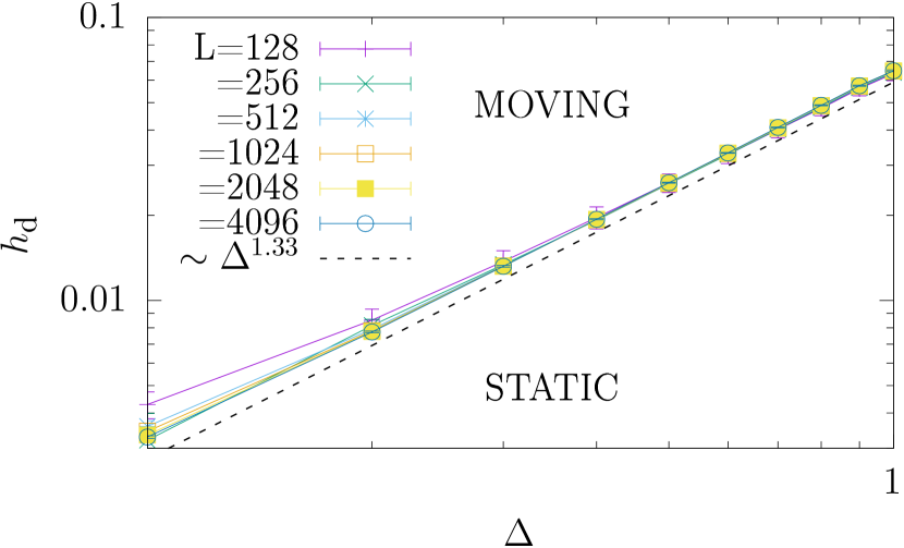
Figure 3: Phase diagram of the domain wall dynamics. A critical field $h_{\tt d}$ as a function of disorder strength $\Delta$ separates the ‘static’ and ‘moving’ phases. It displays a $h_{\tt d}\sim\Delta^{1.33}$ in agreement with the predicted behavior $h_{\tt d}\sim\Delta^{4/(4-d)}(\sigma\delta)^{-d/(4-d)}$ of weak collective pinning theory (dotted line). We display it for different system sizes $L$, finite-size effects are only observed for very small $\Delta$.

We compute the average critical field $h_{\tt d}$ as a function of $\Delta$ for different sizes $L$. Fig.3 shows the power law dependence $h_{\tt d}\sim\Delta^{4/3}$. This result is consistent with Larkin’s prediction for weak collective pinning where $h_{\tt d}\sim{\sigma\delta l_{\tt c}^{-2}}$, with the Larkin length $l_{\tt c}\approx\left({\sigma\delta/\Delta}\right)^{2/(4-d)}$ (note that the microscopic pinning correlation length is the DW width $\delta$). Finally we have [65]:

$$h_{\tt d}\sim\Delta^{4/(4-d)}(\sigma\delta)^{-d/(4-d)},$$ (5)

with $d=1$ in our case. The deviations observed for small $\Delta$ and $L$ can also be explained from the Larkin theory, since for small $\Delta$, $l_{\tt c}$ becomes of the order of $L$. In this case, $l_{\tt c}$ is replaced by $L$, and thus $h_{\tt d}\sim{\sigma\delta L^{-2}}>{\sigma\delta l_{\tt c}^{-2}}$. The fact that the weak collective pinning theory is applicable shows that, at least up to the scale $l_{\tt c}$, the DWs can successfully be described as a smooth elastic interface with univalued displacement field. It also shows that grid-pinning effects are negligible and that depinning is isotropic for the whole $\Delta$ range analyzed (see a detailed discussion in Appendix A).

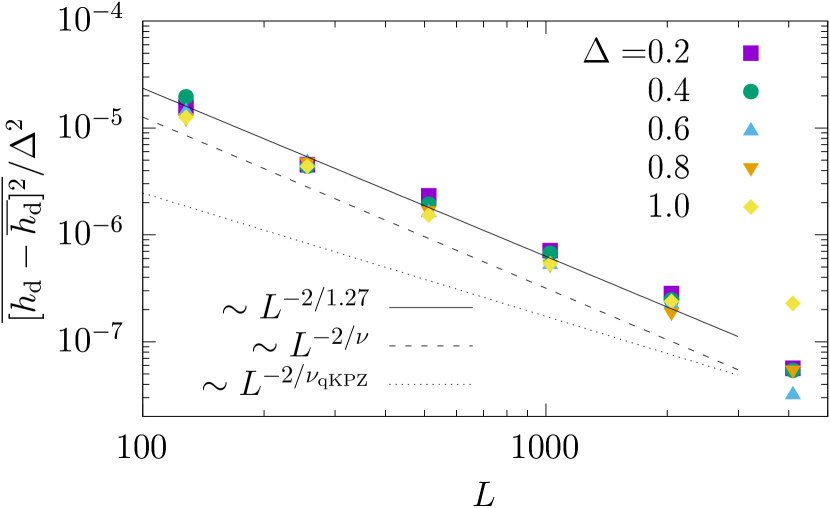
Figure 4: Size dependence of the sample to sample fluctuations of the critical field for different disorder strengths $\Delta$. Data is fairly described $\overline{[h_{\tt d}-\overline{h_{\tt d}}]^{2}}\sim\Delta^{2}L^{1/1.27}$ (solid line), as can be appreciated by fitting the rescaled data. For comparison we plot the scaling expected for the qEW model (dashed-line) and for the qKPZ model (dotted-line).

We have also analyzed the sample to sample fluctuations of the depinning field $h_{\tt d}$. These fluctuations are expected to scale with the size $L$ of the interface as

$$\overline{[h_{\tt d}-\overline{h_{\tt d}}]^{2}}\sim L^{-2/\nu},$$ (6)

For the 1d-qEW model of a SA interface we expect $\nu\approx 4/3$. Quite surprisingly (or maybe not), the same exponent is expected for invasion percolation $\nu^{\tt IP}\approx 4/3$. In Fig.4 we plot the critical field fluctuations as a function of $L$ for different values of $\Delta$. The best fit (solid-line) yields $\overline{[h_{\tt d}-\overline{h_{\tt d}}]^{2}}\sim\Delta^{2}L^{-2/(1.27\pm 0.1)}$, fairly close to $\nu\approx 4/3$ (dashed-line) expected for the 1d-qEW model [26], the invasion percolation model [66] and also to the one observed in 2D-RFIM simulations with strong disorder [60]. In fact, we will argue that this is not just a coincidence.

III.2 Critical Configurations

We now describe the geometrical properties of the configurations corresponding to the critical fields discussed in the previous section.

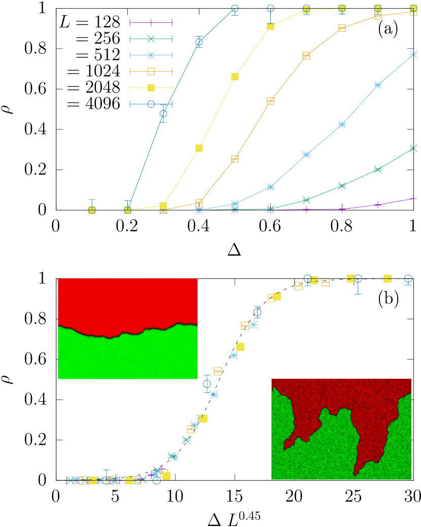
Figure 5: Fraction $\rho$ of multivalued domain walls at the depinning transition. (a) Raw data as a function of disorder strength $\Delta$ and transverse size $L$. (b) Scaled data, showing that $\rho(\Delta,L)\approx\tilde{\rho}(L/l_{\tt o})$ with $l_{\tt o}\sim\Delta^{-1/0.45}$. The inset shows typical domain walls for $L<l_{\tt o}$ (left) and $L>l_{\tt o}$ (right).

III.2.1 Overhangs

For a fixed $L$, depending on $\Delta$, we find that there is a finite probability that the critical configuration presents overhangs (see insets of Fig.5), and also pinch-off loops (see Fig.1). These are detected as multivalued DW displacements with respect to the reference flat initial configuration. We define the overhang probability $\rho$ by counting, for a fixed $L$ and $\Delta$, the fraction of critical DW that presents overhangs for many randomness realizations. In Fig.5(a) we see that always $\rho\to 1$ for large $\Delta$, and $\rho\to 0$ for small $\Delta$. Interestingly, the crossover depends on $L$, and the empiric scaling law $\rho(\Delta,L)\approx\tilde{\rho}(L/l_{\tt o})$, with

$$l_{\tt o}\sim\Delta^{-1/0.45},$$ (7)

decently fits the data for all the $L$ and $\Delta$ values considered, as shown in Fig.5(a). The success of this fit indicates that there exists a crossover length associated to the average overhang size, $l_{\tt o}\sim\Delta^{-1/0.45}$. Since $l_{\tt o}$ diverges when $\Delta\to 0$ and not in a finite value of $\Delta$, our results indicate that there is no transition to a phase of univalued interfaces but a disorder-driven crossover instead, and that DWs are always expected to present overhangs in the thermodynamic limit.

A simple heuristic argument can be used to relate the super-roughness predicted for the qEW model and the occurrence of overhangs. If we assume overhangs appear at the scale $l$ where the extrinsic DW width or “global roughness” $w$ satisfy $dw/dl\sim 1$ with $w\approx\delta(l/l_{\tt c})^{\zeta}$ and $\zeta$ the roughness exponent at that scale, we get

$$l_{\tt o}\sim(l_{\tt c}^{\zeta}/\delta)^{1/(\zeta-1)}\sim\Delta^{-\frac{2\zeta}{(4-d)(\zeta-1)}}$$ (8)

Using that in $d=1$ $l_{\tt c}\sim\Delta^{-2/3}$ we need $\zeta\approx 1.43$ to obtain the observed exponent of $-1/0.45\sim-2.2$ in the scaling of $l_{\tt o}$ with $\Delta$. The value for this effective $\zeta$ remains to be explained, but lies in between the $d=1$ Larkin exponent $\zeta_{\tt L}=3/2$ and the $d=1$ depinning exponent $\zeta\approx 5/4$. More importantly, we note that, to obtain a finite $l_{\tt o}>l_{\tt c}$, the argument requires super-roughening ($\zeta>1$) above $l_{\tt c}$, and suggests that overhangs may not affect the SA geometry if $\zeta<1$ (and for moderate $\Delta$). This may explain why SA two-dimensional interfaces are observed in a three dimensional space at depinning [67], using that $\zeta\approx 0.75$ for the 2d-qEW [24]. The argument then predicts one dimensional SA critical interfaces in the long-range elasticity isotropic depinning case for which $\zeta\approx 0.39$ [30, 31]. In order to test the scaling argument it would be interesting to address these predictions directly in future work.

III.2.2 Roughness exponent

In the previous sections we have shown that DWs at the isotropic depinning transition have always overhangs in the thermodynamic limit. The existence of a large crossover length $l_{\tt o}\sim\Delta^{-2.2}\gg l_{\tt c}$ at weak disorder suggests that the random-manifold regime of the elastic-theory may nevertheless exist at intermediate scales, where the probability of having one or more overhangs in a configuration is low. To test such an hypothesis we next focus on the roughness of the critical configurations.

Standard methods to estimate the roughness exponent $\zeta$ of an interface rely on the existence of a univalued displacement field $u(x)$. We have shown however the interface at a given $x$ can be multievaluated, $\{u_{n}(x)\}_{n=1}^{n=m(x)}$, with $m(x)=1,3,5,\dots$. Hence we define a univalued displacement field

$${\tilde{u}}(x):=\frac{1}{m(x)}\sum_{n=1}^{m(x)}u_{n}(x).$$ (9)

This particular choice coincides with the usual univalued interface if $m(x)=1\;\forall x$, but in the presence of overhangs it introduces artificial discontinuities in ${\tilde{u}}(x)$. Besides this warning, it is an operationally well defined regularization, not only for simulation but also for experiments. A convenient way to obtain the roughness exponent at different length scales is through the structure factor

$$S(q):=\overline{\left|\sum_{x=1}^{L}e^{iqx}{\tilde{u}}(x)\right|^{2}}\sim\frac{1}{q^{1+2\zeta}}.$$ (10)

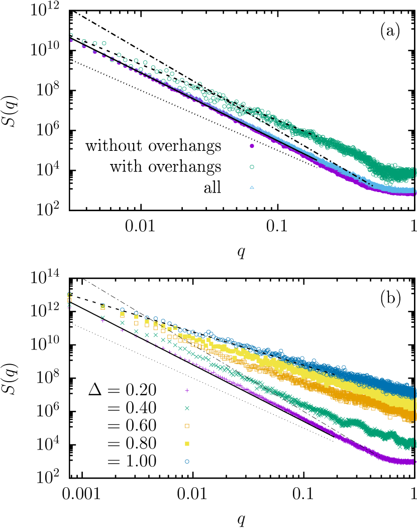
Figure 6: Disorder averaged structure factor $S(q)$ of domain wall critical configurations. Data obtained for a system size $L=8192$ (corresponding to a grid of ${8192^{2}\simeq 6.7\times 10^{7}}$ sites). (a) $S(q)$ averaged over configurations with overhangs, without overhangs, and averaged over all configurations (180 samples), for a fixed disorder strength $\Delta=0.2$. Lines are guides to the eye and display pure power-laws for $\zeta=1.2$ (solid-line) $\zeta=1$ (dotted-line), and $\zeta=0.9$ (dashed-line). (b) $S(q)$ averaged over all sampled critical configurations for increasing values of disorder strength $\Delta$ (180 samples for $\Delta=0.2$, 50 samples for $\Delta\!>\!0.2$). Guides-to-the-eye lines display pure power-laws for $\zeta\!=\!1.2$ (solid-line) and $\zeta\!=\!0.5$ (dashed-line).

In Fig.6(a) we show $S(q)$ for $\Delta=0.2$ and $L=8192$. For these parameters $\rho\approx 0.2$, so -on average- one over five critical configurations is expected to have one or more overhangs. If we separate the contributions from interfaces with and without overhangs we can observe marked differences. For low $q$, in the case without overhangs, we can very accurately fit an exponent $\zeta\approx 1.2$ (solid-line) which is compatible with the reported values $\zeta\approx 1.25$ for the 1d-qEW at depinning [5]. In the case with overhangs we can reasonably fit (dashed-line) an effective exponent $\zeta_{\tt eff}=0.9$ over the low-$q$ region, even if overhangs have an important effect for the whole range of $q$. For the chosen value $\Delta=0.2$, the average over all configurations (with and without overhangs) is dominated by the ones without overhangs. Nevertheless, as we increase $\Delta$ (or increase $L$) the configurations with overhangs dominate the average. In Fig.6(b) we show the results for increasing values of $\Delta$, the value of $\zeta_{\tt eff}$ decreases with increasing $\Delta$ and tends to an exponent $\zeta_{\tt eff}\approx 0.5$ .

The results of Fig.6 support the applicability of the 1d-qEW model to describe DW at depinning to scales below $l_{\tt o}$, where overhangs are rare. On the other hand, overhangs produce lower effective roughness exponents. These must be interpreted carefully because they depend on our particular way to define ${\tilde{u}}$ in Eq.(9). This result thus stresses the importance of a conscious interpretation of experimental data when $L>l_{\tt o}$. More importantly, it stresses the importance of estimating quantitatively the crossover length $l_{\tt o}$, both in experiments and simulations at the isotropic depinning transition.

III.2.3 Overhangs size scaling

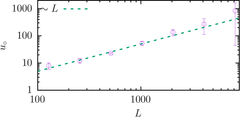
Figure 7: Typical linear size of overhangs $u_{\tt o}$ (Eq.(11)) in the displacement direction as a function of the system size $L$ for $\Delta=1$. The dashed-line is a guide to the eye with slope $\propto L$.

In Fig.6(b) we can see that for strong disorder $\zeta_{\tt eff}\approx 0.5$, compatible with simple thermal roughening. One can interrogate whether this result is an artifact introduced by the regularization of Eq.(9) or rather an indication that a SA interface is emerging in spite of the presence of overhangs. In order to answer this question, with our model we analyze how the typical size of overhangs scales with the system linear size $L$. To do this we first define

$$u_{\tt o}^{2}:=\overline{\frac{1}{L}\sum_{x=1}^{L}\left[\sum_{n=1}^{m(x)}\frac{u_{n}(x)^{2}}{m(x)}-\left(\sum_{n=1}^{m(x)}\frac{u_{n}(x)}{m(x)}\right)^{2}\right]}.$$ (11)

The quantity between brackets $[\dots]$ is identically zero if there is no overhang at $x$ (since in that case $m(x)=1$), and it is of the order of the overhang size squared otherwise (i.e. the variance of the multiple values of $u(x)$). Therefore, $u_{\tt o}$ gives the typical size of the overhangs in a given configuration (note that for a univalued function $u_{\tt o}=0$ regardless of its roughness).

In Fig. 7 we show that for $\Delta=1$, $u_{\tt o}$ scales approximately linearly with $L$. This demonstrates that overhangs are relevant in the thermodynamic limit and can not be eliminated by coarse-graining. The snapshot shown in the right side inset of Fig.5 illustrates this result for a particular critical configuration. Therefore, the roughness exponent $\zeta_{\tt eff}$ cannot be related to any emerging SA scale invariant. On the other hand, this suggests that overhangs allow to recover the rotational symmetry, as they promote wandering of the local orientation of the DW. So that the final picture for the roughness of the DW is: SA qEW $\to$ finite size crossover $\to$ SS (invasion percolation depinning), as larger length scales are tested.

IV Conclusions

In summary, using an accurate algorithm we showed that critical configurations at the isotropic depinning transition of one dimensional DWs always present thermodynamically large overhangs in the thermodynamic limit. Rotational invariance is thus not broken at the isotropic depinning transition of $d=1$ dimensional DWs in $d=2$ random media. We find nevertheless a crossover length below which the predictions of the elastic theory of univalued interfaces predictions are well satisfied, including the qEW super-roughness. This extends the current theoretical understanding of depinning and reconciles it with many experimental observations where compatibility with the predictions for the 1d-qEW depinning universality class is found. We thus propose a full picture for the DW depinning in isotropic two dimensional media which we hope will motivate further experimental and theoretical research on the depinning transition.

Our results could be relevant for experiments. While so far they can only compare at a qualitative level, the long standing statistical physics questions addressed in our work are important even for the experimental protocol conception and data analysis. For instance, work on magnetic DWs in the lab sometimes avoid including in the analysis non-univalued pieces of interface and/or disregard pinch-offs as rare impurities related occurrences. We could now argue that those are not things to avoid, that they make part of the isotropic depinning theory and play a role in preserving the DW characteristics. We then hope that our work could motivate a new look to experimental data (even the already existent one), perhaps not only in magnetic domain walls but also on different experimental realizations of 1D DWs in 2D random media.

Appendix A Control of lattice effects

In order to solve Eq.(1) numerically, a finite difference scheme based on an anisotropic regular lattice is typically used. If one wants to simulate isotropic depinning, it is important to assure that the effect of the discretization is negligible. This effect can be greatly reduced and put under control by choosing the DW width $\delta$ large enough. The smoother is the interface, the weaker is the effect of the mesh. Yet, a very wide domain wall requires larger systems to study the critical behaviour. To choose a reasonable value of $\delta\approx\sqrt{c/\epsilon_{0}}$, we perform two numerical experiments.

Figure 8: Blowing an initially circular domain with a constant field $h=0.1$, for $\epsilon_{0}=1$ and different values of $c$ as indicated, corresponding to different values of the DW width $\delta\approx\sqrt{c/\epsilon_{0}}$. Lines of different colors corresponds to DW configurations at regularly distributed times.

First, we test the relevance of the anisotropic effect induced by the mesh by blowing an initially circular domain in the absence of disorder. We seed a circular domain at the center of the system and directly solve the dynamics of Eq.(1) at a constant field $h=0.1$, for different DW widths by fixing $\epsilon_{0}=1$ and varying $c$. In Fig.8 we observe that small values of $c$ ($c=0.2$ and $c=0.5$) lead to an anisotropic growth that deviates from the circular shape. Further, one can see that the growth mean velocity is changing due to the mesh effect, since concentric lines correspond to regularly distributed times and they come closer to each other. For $c=0.2$ the artificial periodic pinning is even able to pin the interface into a square metastable configuration. Fortunately, at larger values of $c$ the undesired anisotropic effect rapidly vanishes ($c=0.75$ displays circular configurations and for $c=1$ we cannot detect any sign of anisotropy). Note that in the latter case, $\delta\approx 1$, a width comparable with the lattice spacing. The uncorrelated disorder increases system isotropy because rough DWs cannot coherently couple to the underlying periodic potential.

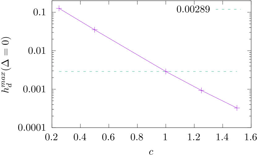
Figure 9: Maximum depinning field $h_{\tt d}^{max}$ in the absence of disorder ($\Delta=0$) due to the effect of the square numerical mesh, vs the order parameter elastic constant $c$. The dashed-line indicates $h_{\tt d}^{max}$ for the parameters used to obtain our results in the main text.

To go further, we also compute the pinning field $h_{\tt d}$ induced purely from the mesh in the absence of disorder ($\Delta=0$) and compare it with the whole range of $h_{\tt d}$ values that we analyzed in Fig.3 for different disorder strengths $\Delta$. As for the case $c=0.2$, $h=0.1$, the maximum pinning field $h_{\tt d}^{\max}(\Delta=0)$ is associated to a square DW. In Fig.9 we show $h_{\tt d}^{\max}(\Delta=0)$, computed using our exact algorithm, as a function of the elastic constant $c$. We can observe that it decreases approximately exponentially with increasing $c$, (i.e increasing the DW width). In particular, for the choice $c=1$ that we adopted to obtain most of the results in our work, we get $h_{\tt d}^{max}(\Delta=0)\approx 0.00289$, much smaller than the critical field obtained for the weakest disordered considered ($\Delta=0.1$). Therefore, we conclude the mesh pinning does not affect our results. For even smaller $\Delta$ values, it may be necessary to increase the DW’s intrinsic width $\delta\sim\sqrt{c/\epsilon_{0}}$, either increasing $c$ or decreasing $\epsilon_{0}$. Fig.9 can be used as a general guide for that.

In summary, we find that anisotropic effects can be kept under control for any disorder strength. Our method thus constitutes an essential improvement over models of discrete scalar fields: In the 2D-RFIM DWs are always sharp. In particular, in the limit of weak disorder, square domains are not avoidable already at $\Delta\sim 1$ [60, 61]. Fig.3 shows that these kind of effects are absent in our simulations. Therefore, our approach allows to test the prediction of the elastic theory in isotropic depinning.

References

- Kardar [1998] M. Kardar, Physics Reports 301, 85 (1998).
- Nattermann and Scheidl [2000] T. Nattermann and S. Scheidl, Advances in Physics 49, 607 (2000).
- Fisher [1998] D. S. Fisher, Physics Reports 301, 113 (1998).
- Wiese [2022] K. J. Wiese, Reports on Progress in Physics 85, 086502 (2022).
- Ferré et al. [2013] J. Ferré, P. J. Metaxas, A. Mougin, J.-P. Jamet, J. Gorchon, and V. Jeudy, Comptes Rendus Physique 14, 651 (2013), disordered systems / Systèmes désordonnés.
- Kleemann et al. [2007] W. Kleemann, J. Rhensius, O. Petracic, J. Ferré, J. P. Jamet, and H. Bernas, Phys. Rev. Lett. 99, 097203 (2007).
- Paruch and Guyonnet [2013] P. Paruch and J. Guyonnet, Comptes Rendus Physique 14, 667 (2013), disordered systems / Systèmes désordonnés.
- Bonamy et al. [2008] D. Bonamy, S. Santucci, and L. Ponson, Phys. Rev. Lett. 101, 045501 (2008).
- Ponson [2009] L. Ponson, Phys. Rev. Lett. 103, 055501 (2009).
- Le Priol et al. [2020] C. Le Priol, J. Chopin, P. Le Doussal, L. Ponson, and A. Rosso, Phys. Rev. Lett. 124, 065501 (2020).
- Joanny and de Gennes [1984] J. F. Joanny and P. G. de Gennes, The Journal of Chemical Physics 81, 552 (1984).
- Moulinet et al. [2004] S. Moulinet, A. Rosso, W. Krauth, and E. Rolley, Phys. Rev. E 69, 035103 (2004).
- Doussal et al. [2009] P. L. Doussal, K. J. Wiese, S. Moulinet, and E. Rolley, Europhysics Letters 87, 56001 (2009).
- Jagla and Kolton [2010] E. A. Jagla and A. B. Kolton, Journal of Geophysical Research: Solid Earth 115 (2010).
- Jagla et al. [2014] E. A. Jagla, F. m. c. P. Landes, and A. Rosso, Phys. Rev. Lett. 112, 174301 (2014).
- Kolton et al. [2013] A. B. Kolton, S. Bustingorry, E. E. Ferrero, and A. Rosso, Journal of Statistical Mechanics: Theory and Experiment 2013, P12004 (2013).
- Cao et al. [2018] X. Cao, S. Bouzat, A. B. Kolton, and A. Rosso, Phys. Rev. E 97, 022118 (2018).
- Ferrero et al. [2013a] E. E. Ferrero, S. Bustingorry, A. B. Kolton, and A. Rosso, Comptes Rendus Physique 14, 641 (2013a).
- Le Doussal et al. [2002] P. Le Doussal, K. J. Wiese, and P. Chauve, Phys. Rev. B 66, 174201 (2002).
- Fedorenko and Stepanow [2003] A. A. Fedorenko and S. Stepanow, Phys. Rev. E 67, 057104 (2003).
- Leschhorn [1993] H. Leschhorn, Physica A: Statistical Mechanics and its Applications 195, 324 (1993).
- Leschhorn et al. [1997] H. Leschhorn, T. Nattermann, S. Stepanow, and L.-H. Tang, Annalen der Physik 509, 1 (1997).
- Roters et al. [1999] L. Roters, A. Hucht, S. Lübeck, U. Nowak, and K. D. Usadel, Phys. Rev. E 60, 5202 (1999).
- Rosso et al. [2003] A. Rosso, A. K. Hartmann, and W. Krauth, Phys. Rev. E 67, 021602 (2003).
- Rosso et al. [2007] A. Rosso, P. Le Doussal, and K. J. Wiese, Phys. Rev. B 75, 220201 (2007).
- Ferrero et al. [2013b] E. E. Ferrero, S. Bustingorry, and A. B. Kolton, Phys. Rev. E 87, 032122 (2013b).
- Ferrero et al. [2013c] E. E. Ferrero, S. Bustingorry, and A. B. Kolton, Phys. Rev. E 87, 069901 (2013c).
- Ramanathan and Fisher [1998] S. Ramanathan and D. S. Fisher, Phys. Rev. B 58, 6026 (1998).
- Zapperi et al. [1998] S. Zapperi, P. Cizeau, G. Durin, and H. E. Stanley, Phys. Rev. B 58, 6353 (1998).
- Rosso and Krauth [2002] A. Rosso and W. Krauth, Phys. Rev. E 65, 025101 (2002).
- Duemmer and Krauth [2007] O. Duemmer and W. Krauth, Journal of Statistical Mechanics: Theory and Experiment 2007, P01019 (2007).
- Laurson et al. [2013] L. Laurson, X. Illa, S. Santucci, K. Tore Tallakstad, K. J. Måløy, and M. J. Alava, Nature Communications 4, 2927 (2013).
- Boltz and Kierfeld [2014] H.-H. Boltz and J. Kierfeld, Phys. Rev. E 90, 012101 (2014).
- Tang et al. [1995] L.-H. Tang, M. Kardar, and D. Dhar, Phys. Rev. Lett. 74, 920 (1995).
- Fedorenko et al. [2006] A. A. Fedorenko, P. Le Doussal, and K. J. Wiese, Phys. Rev. E 74, 041110 (2006).
- Bustingorry et al. [2010] S. Bustingorry, A. B. Kolton, and T. Giamarchi, Phys. Rev. B 82, 094202 (2010).
- Amaral et al. [1994] L. A. N. Amaral, A.-L. Barabási, and H. E. Stanley, Phys. Rev. Lett. 73, 62 (1994).
- Rosso and Krauth [2001] A. Rosso and W. Krauth, Phys. Rev. Lett. 87, 187002 (2001).
- Goodman and Teitel [2004] T. Goodman and S. Teitel, Phys. Rev. E 69, 062105 (2004).
- Le Doussal and Wiese [2003] P. Le Doussal and K. J. Wiese, Phys. Rev. E 67, 016121 (2003).
- Chen et al. [2015] Y. J. Chen, S. Zapperi, and J. P. Sethna, Phys. Rev. E 92, 022146 (2015).
- Mukerjee and Wiese [2023] G. Mukerjee and K. J. Wiese, Phys. Rev. E 107, 054137 (2023).
- Mukerjee et al. [2023] G. Mukerjee, J. A. Bonachela, M. A. Muñoz, and K. J. Wiese, Phys. Rev. E 107, 054136 (2023).
- Ioffe and Vinokur [1987] L. B. Ioffe and V. M. Vinokur, Journal of Physics C: Solid State Physics 20, 6149 (1987).
- Nattermann [1990] T. Nattermann, Phys. Rev. Lett. 64, 2454 (1990).
- Chauve et al. [2000] P. Chauve, T. Giamarchi, and P. Le Doussal, Phys. Rev. B 62, 6241 (2000).
- Kolton et al. [2006a] A. B. Kolton, A. Rosso, T. Giamarchi, and W. Krauth, Phys. Rev. Lett. 97, 057001 (2006a).
- Kolton et al. [2009] A. B. Kolton, A. Rosso, T. Giamarchi, and W. Krauth, Phys. Rev. B 79, 184207 (2009).
- Ferrero et al. [2017] E. E. Ferrero, L. Foini, T. Giamarchi, A. B. Kolton, and A. Rosso, Phys. Rev. Lett. 118, 147208 (2017).
- Ferrero et al. [2021] E. E. Ferrero, L. Foini, T. Giamarchi, A. B. Kolton, and A. Rosso, Annual Review of Condensed Matter Physics 12, 111 (2021).
- Grassi et al. [2018] M. P. Grassi, A. B. Kolton, V. Jeudy, A. Mougin, S. Bustingorry, and J. Curiale, Phys. Rev. B 98, 224201 (2018).
- Lemerle et al. [1998] S. Lemerle, J. Ferré, C. Chappert, V. Mathet, T. Giamarchi, and P. Le Doussal, Phys. Rev. Lett. 80, 849 (1998).
- Jeudy et al. [2018] V. Jeudy, R. Díaz Pardo, W. Savero Torres, S. Bustingorry, and A. B. Kolton, Phys. Rev. B 98, 054406 (2018).
- Jeudy et al. [2016] V. Jeudy, A. Mougin, S. Bustingorry, W. Savero Torres, J. Gorchon, A. B. Kolton, A. Lemaître, and J.-P. Jamet, Phys. Rev. Lett. 117, 057201 (2016).
- Albornoz et al. [2021] L. J. Albornoz, E. E. Ferrero, A. B. Kolton, V. Jeudy, S. Bustingorry, and J. Curiale, Phys. Rev. B 104, L060404 (2021).
- Caballero et al. [2018] N. B. Caballero, E. E. Ferrero, A. B. Kolton, J. Curiale, V. Jeudy, and S. Bustingorry, Phys. Rev. E 97, 062122 (2018).
- Caballero et al. [2020] N. Caballero, E. Agoritsas, V. Lecomte, and T. Giamarchi, Phys. Rev. B 102, 104204 (2020).
- Guruciaga et al. [2021] P. C. Guruciaga, N. Caballero, V. Jeudy, J. Curiale, and S. Bustingorry, Journal of Statistical Mechanics: Theory and Experiment 2021, 033211 (2021).
- Caballero [2021] N. Caballero, Journal of Statistical Mechanics: Theory and Experiment 2021, 103207 (2021).
- Ji and Robbins [1991] H. Ji and M. O. Robbins, Phys. Rev. A 44, 2538 (1991).
- Koiller et al. [1992] B. Koiller, H. Ji, and M. O. Robbins, Phys. Rev. B 46, 5258 (1992).
- Rosso and Krauth [2005] A. Rosso and W. Krauth, Computer Physics Communications 169, 188 (2005), proceedings of the Europhysics Conference on Computational Physics 2004.
- Note [1] The computational cost of the present algorithm is equivalent to the one applied to two-dimensional univalued interfaces (only the nonlinear force changes). We refer the reader to Ref. [24] for a discussion about its performance compared with the direct integration of the equation of motion of the 2d interface (i.e. the equivalent to Eq.(1)).
- Kolton et al. [2006b] A. B. Kolton, A. Rosso, E. V. Albano, and T. Giamarchi, Phys. Rev. B 74, 140201 (2006b).
- Blatter et al. [1994] G. Blatter, M. V. Feigel’man, V. B. Geshkenbein, A. I. Larkin, and V. M. Vinokur, Rev. Mod. Phys. 66, 1125 (1994).
- Maslov [1995] S. Maslov, Phys. Rev. Lett. 74, 562 (1995).
- Clemmer and Robbins [2019] J. T. Clemmer and M. O. Robbins, Phys. Rev. E 100, 042121 (2019).
- Note [2] It is worth noting that the decrease of with increasing is similar to the behavior reported in [69] for the spectral roughness exponent in the 2D-RFIM using the Monte Carlo method.
- Qin et al. [2012] X. P. Qin, B. Zheng, and N. J. Zhou, Journal of Physics A: Mathematical and Theoretical 45, 115001 (2012).