Explicit Solutions in Isotropic Planar Elastostatics

Abstract.

Addressing the intricate challenges in plane elasticity, especially with non-vanishing traction and complex geometries, requires innovative methods. This paper offers a novel approach, drawing inspiration from the Neumann problem for the inhomogeneous Cauchy-Riemann problem. Our method caters to domains that are conformally equivalent to a unit disk or annulus and emphasizes deriving explicit solutions for the displacement field rather than the stress tensor, differentiating it from most traditional methods. We explore solutions for specific traditional cases to demonstrate its efficacy, such as a cardioid domain, a ring domain with a shifted hole, and a gear-like structure. This work augments the existing toolbox for researchers and practitioners addressing isotropic planar elastostatics challenges, presenting a unified and flexible approach.

1. Introduction

The study of plane elasticity in a domain $\Omega$ has a vibrant history in the engineering and physical sciences. The domain $\Omega$ symbolizes a symmetric, isotropic, and linear material whose associated elastic behavior is traditionally captured by two equations:

$$-\nabla\cdot\sigma(\boldsymbol{u}) =\boldsymbol{f}\text{ in }\Omega,$$ (1.1)

$$\sigma(\boldsymbol{u})\cdot\boldsymbol{\hat{n}} =\boldsymbol{g}\text{ on }\partial\Omega.$$

In these equations, $\sigma(\boldsymbol{u})$ refers to the stress tensor and $\boldsymbol{f}$ denotes the force. The stress tensor $\sigma(\boldsymbol{u})$ is then described by $\sigma(\boldsymbol{u})=2\mu\varepsilon(\boldsymbol{u})+\lambda(\nabla\cdot\boldsymbol{u})\boldsymbol{1}$ with $\boldsymbol{1}$ being the $2\times 2$ identity matrix, and $\varepsilon(\boldsymbol{u})$ is the strain tensor given as the symmetric part of the Jacobian of $\boldsymbol{u}$. Furthermore, $\mu,\lambda$ are the associated Lamé parameters and the force $\boldsymbol{f}$ can also be rewritten in terms of a specific force $\boldsymbol{F}$ as $\boldsymbol{f}=\rho\boldsymbol{F}$ using the density $\rho$ of the material.

These equations are typically addressed using numerical solutions like finite element or boundary element methods, especially in applications. However, complexities in geometric properties often pose substantial difficulties. Hence, the derivation of explicitly represented solutions has been an area of considerable focus.

The use of complex functions in plane elastic problems was initiated in the work of Kolosov in 1909 [15] following the method of Kirsch, which focused on the solution around a circular hole [14]. Several authors have extended this work, most famously Mushkelishvili [20] to more general domains and Westergaard [25] to crack problems. Both of these methods build on representing the stress tensor in terms of Airy potential functions, allowing the stresses to be solved. It is then possible, in some instances, to solve for the displacement via these stresses. It was also shown by Yun [27] in the 90s that it is possible to obtain potential-based solutions to the elasticity problem starting with the Navier equation.

However, these approaches do come with their drawbacks. In this work, we have demonstrated a novel method for solving a broad class of problems in plane elasticity. In particular, we have shown a clear correspondence between the well-studied Cauchy-Riemann problem and the problem of linear elasticity in bounded plane domains, which are conformally equivalent to either the disk or an annulus. Although reminiscent of other complex methods, such as the ones in [7, 15, 20, 21], our method yields a more direct approach as well as an explicit formula for the displacement field rather than the stress tensor.

An additional area for improvement that has emerged with this method pertains to the challenges that arise when considering ring-shaped domains. These structures are common in many engineering constructions, such as, e.g., gears and ring bearings. To study the deformation and internal stress distribution in these, one often resorts to using bipolar coordinates, as done by, e.g., Chen et al. in [5, 6] or Alaci, Ciornei, and Romanu in [1]. We shall also consider a simple notch problem that has turned out to pose a problem historically when using Airy potentials due to singularities at the corner [12, 26].

Motivated by these challenges, this paper outlines a new method for obtaining integral representations of the solution to (1.1) in domains which can be obtained as the image of conformal maps from either a unit disk or an annulus. We accomplish this by leveraging the established knowledge of the Neumann problem for the inhomogeneous Cauchy-Riemann problem and the known representations of its solutions due to Begehr and Vaitekhovich [3, 24].

Our main results, encapsulated in Theorem 3.4 for simply connected domains $\Omega$ that are conformally equivalent to the unit disk $\mathbb{D}$ and Theorem  4.3 for domains $\Omega$ that are conformally equivalent to the annulus $\mathbb{A}_{r}=\{z\in\mathbb{C}:r<|z|<1\}$, provide advancements in solving plane elasticity problems. In Section 5, we further illustrate the applicability of our method by demonstrating solutions to a notch problem in a cardioid domain, a ring domain with a shifted hole, and a gear-like domain, underscoring the wide-ranging potential of our approach.

When analyzing the method presented in this paper, it is crucial to contextualize it within the broader landscape of existing techniques. A natural point of comparison is the classical method, commonly referred to as Kolosov’s method or the classical complex method [20]. This method boasts the ability to explicitly determine stress values across diverse domains. A disadvantage of Kolosov’s method is that it demands the conformal map to be rational. Although attempts have been made to dispense with this necessity by seeking approximations through rational functions, these endeavors have proven cumbersome and not particularly fruitful, as Neuber [21] pointed out. Moreover, the classical method often necessitates deriving the primary ingredients for individual problems since a comprehensive framework for general force classes or domains is absent. This contrasts with our method, which sets conditions on general classes of both loads and domains. Finally, when comparing with the real integral equation method [7] and the Somigliana method [22], a distinct advantage of our approach becomes evident as it sidesteps the need to introduce intermediary entities like integral operators or layer potentials.

2. Notation and preliminaries

In this section, we introduce several essential concepts and notation used throughout the paper. Our focus is on the elastostatic equation in a bounded planar domain $\Omega$ consisting of a specific material with associated Lamé parameters $\mu,\lambda$, which describe the elastic properties of the material. The problem is typically presented in its divergence form (1.1). The displacement field $\boldsymbol{u}$ describes the deformation of the domain, $\boldsymbol{f}$ denotes a body force acting on the domain, and $\boldsymbol{g}$ represents the boundary traction on $\partial\Omega$. The force $\boldsymbol{f}$ can also be rewritten in terms of a specific force $\boldsymbol{F}$ as $\boldsymbol{f}=\rho\boldsymbol{F}$. The representation of the force will turn out to be important, hence we shall consider the standard representation $\boldsymbol{F}=\nabla\phi+\nabla\times\boldsymbol{A}$.

If $\Omega$ has multiple boundaries, $\boldsymbol{g}$ is a piecewise-defined function. The stress-tensor $\sigma(\boldsymbol{u})$ is a matrix derived from the displacement field $\boldsymbol{u}$, defined as $\sigma(\boldsymbol{u})=2\mu\varepsilon(\boldsymbol{u})+\lambda(\nabla\cdot\boldsymbol{u})\boldsymbol{1}$ with $\boldsymbol{1}$ being the 2-by-2 identity matrix, and $\varepsilon(\boldsymbol{u})$ representing the strain tensor. The strain tensor is the symmetric part of the Jacobian of $\boldsymbol{u}$, or equivalently $\varepsilon(\boldsymbol{u})=\frac{\nabla\boldsymbol{u}+(\nabla\boldsymbol{u})^{T}}{2}$. For an in-depth introduction to this problem and its generalizations, we refer the reader to Chapter 7 in [19].

The divergence form, although compact, can be challenging to work with. Thus, it is common to recast the problem into an explicit second-order form, known as the Navier equation or the Navier-Cauchy equation:

$$(\mu+\lambda)\nabla(\nabla\cdot\boldsymbol{u})+\mu\nabla^{2}\boldsymbol{u}+\rho\boldsymbol{F}=0.$$

Here, $\nabla^{2}$ denotes the Laplacian, and the body force $\boldsymbol{f}$ has been rewritten in terms of a specific force $\boldsymbol{F}$ using the material density $\rho$. This conversion is carried out in the proof of Theorem 3.2 and will be needed to link the above problem with the Cauchy-Riemann problem.

It is worth noting the relationship between the above equation and dynamical systems. This equation can be regarded as the steady-state equation for elastodynamics. Adding the term $\rho\frac{\partial^{2}\boldsymbol{u}}{\partial t^{2}}$ to the right-hand side yields the standard equation describing the dynamical behavior of elastic solids. Therefore, if the equation is separable, the results in this paper may facilitate the construction of dynamical solutions.

Next, we recall the notation for the classical Wirtinger derivatives:

$$\partial_{\overline{z}}=(\partial_{x}+i\partial_{y})/2\quad\text{ and }\quad\partial_{z}=(\partial_{x}-i\partial_{y})/2.$$

For a planar set $E$, we denote by $\mathcal{C}(E;\mathbb{C})$ the space of continuous complex-valued functions defined on $E$. For a real number $\alpha$ such that $0<\alpha<1$, the notation $\mathcal{C}^{\alpha}(E;\mathbb{C})$ denotes the space of $\alpha$-Hölder continuous functions. These are functions $\psi$ that satisfy

$$|\psi(z)-\psi(\zeta)|\leq C|z-\zeta|^{\alpha},$$

for some $C>0$. For positive integer values of $k$, $\mathcal{C}^{k}(E;\mathbb{C})$ denotes functions whose partial derivatives up to order $k$ are continuous in $E$ and $\mathcal{C}^{k}(\overline{E},\mathbb{C})$ if they are $\mathcal{C}^{k}$ in a neighbourhood around $E$. Lastly, the notation $\mathcal{C}^{1,\alpha}(E;\mathbb{C})$ denotes functions whose first partial derivatives belong to the space $\mathcal{C}^{\alpha}(E;\mathbb{C})$.

3. The case of simply connected domains

In this section, we will demonstrate that the plane elasticity problem, as shown in (1.1), considered in a simply connected domain, can be understood as an equivalent Neumann problem for the inhomogeneous Cauchy-Riemann equations within the same domain as viewed in $\mathbb{C}$. First, we need to recall the following result.

Theorem 3.1.

Let $\psi\in\mathcal{C}^{\alpha}(\overline{\mathbb{D}};\mathbb{C})$, $0<\alpha<1$, $\gamma\in\mathcal{C}(\partial\mathbb{D};\mathbb{C})$, $c\in\mathbb{C}$. The Neumann problem for the inhomogeneous Cauchy-Riemann equation in the unit disc

$$\partial_{\overline{z}}w =\psi\text{ in }\mathbb{D},$$

$$\partial_{\nu}w =\gamma\text{ on }\partial\mathbb{D}$$

$$w(0) =c$$

is solvable if and only if for $|z|<1$

$$\frac{1}{2\pi i}\int_{|\zeta|=1}\gamma(\zeta)\frac{d\zeta}{(1-\overline{z}\zeta)\zeta}+\frac{1}{2\pi i}\int_{|\zeta|=1}\psi(\zeta)\frac{d\overline{\zeta}}{1-\overline{z}\zeta}+\frac{1}{\pi}\int_{|\zeta|<1}\frac{\overline{z}\psi(\zeta)}{(1-\overline{z}\zeta)^{2}}d\xi d\eta=0.$$

The unique solution is then given by

$$w=c-\frac{1}{2\pi i}\int_{|\zeta|=1}\big{(}\gamma(\zeta)-\overline{\zeta}\psi(\zeta)\big{)}\log(1-z\overline{\zeta})\frac{d\zeta}{\zeta}-\frac{1}{\pi}\int_{|\zeta|<1}\frac{z\psi(\zeta)}{\zeta(\zeta-z)}d\xi d\eta.$$

Proof.

See Theorem 11 in [3]. ∎

Next, we turn to the first contribution of this paper.

Theorem 3.2.

Let $\mathbb{D}$ denote the unit disk and $\mu,\lambda$ its associated Lamé parameters. Let $\phi,\boldsymbol{A}=A\boldsymbol{\hat{z}}$, where $\phi,A$, are $\mathcal{C}^{2}$ in a neighborhood of $\mathbb{D}$, be potentials and $\boldsymbol{F}=\leavevmode\nobreak\ \nabla\phi+\nabla\times\boldsymbol{A}$ denote the associated specific loading force. Then, the existence of a displacement field $\boldsymbol{u}$ to the following problem

$$- \nabla\cdot\sigma(\boldsymbol{u})=\rho\boldsymbol{F}\text{ in }\mathbb{D}$$

$$\sigma(\boldsymbol{u})\cdot\boldsymbol{\hat{n}}=\boldsymbol{g}\text{ on }\partial\mathbb{D}$$ (3.1)

$$\boldsymbol{u}(0)=\boldsymbol{0}$$

is equivalent to the function $w=u_{1}-iu_{2}$ solving the following Neumann problem for the inhomogeneous Cauchy-Riemann equation

$$\partial_{\overline{z}}w =\frac{\psi}{2}\text{ in }\mathbb{D}$$

$$\partial_{\nu}w =\gamma\text{ on }\partial\mathbb{D}$$ (3.2)

$$w(0) =0,$$

where $\psi=-\frac{\rho}{2\mu+\lambda}\phi-i\frac{\rho}{\mu}A$, $\gamma=\frac{1}{2\mu}(g_{1}-ig_{2})+\frac{\rho}{2\mu}\overline{\zeta}\big{(}\nu\phi-iA\big{)}$, and $\nu=\frac{\lambda}{\lambda+2\mu}$ is the Poisson ratio.

Proof.

We show that (3.1) implies (3.2). The reverse implication is shown similarly. Assume (3.1) holds. By the definition of the stress tensor $\sigma(\boldsymbol{u})$, $\boldsymbol{u}$ also satisfies

$$(\mu+\lambda)\nabla(\nabla\cdot\boldsymbol{u})+\mu\nabla^{2}\boldsymbol{u}+\rho\boldsymbol{F}=0.$$ (3.3)

This follows from explicitly writing out the components of $\varepsilon(\boldsymbol{u})$ and $\nabla\cdot\boldsymbol{u}$. Assuming planarity, i.e., $\boldsymbol{u}=\boldsymbol{u}(x,y)$ and $\boldsymbol{u}\cdot\boldsymbol{\hat{z}}=0$, we use the identity $\nabla^{2}\boldsymbol{u}=\nabla(\nabla\cdot\boldsymbol{u})-\nabla\times(\nabla\times\boldsymbol{u})$ to arrive at

$$(\mu+\lambda)\nabla(\nabla\cdot\boldsymbol{u})+\mu\nabla^{2}\boldsymbol{u}+\rho\boldsymbol{F}=(2\mu+\lambda)\nabla(\nabla\cdot\boldsymbol{u})-\mu\nabla\times(\nabla\times\boldsymbol{u})+\rho\boldsymbol{F}=0\,,$$

which allows us to make the associations

$$\rho\phi=-(2\mu+\lambda)\nabla\cdot\boldsymbol{u}\quad\text{ and }\quad\rho\boldsymbol{A}=\mu(\nabla\times\boldsymbol{u})$$

within the disk. Note that this association is possible, and it is unique since the data is assumed to be $\mathcal{C}^{2}$ in a neighborhood around the closed disk. Hence, there exists boundary values $\phi^{*}=\phi|_{\partial\mathbb{D}},\boldsymbol{A}^{*}=\boldsymbol{A}|_{\partial\mathbb{D}}$ fixing the Helmholtz decomposition. Expanding these equalities in terms of components and making substitutions $u_{1}=w_{1},u_{2}=-w_{2}$ in the second equation yields

$$\partial_{x}u_{1}+\partial_{y}u_{2}=-\frac{\rho}{2\mu+\lambda}\phi,$$

$$\partial_{x}u_{2}-\partial_{y}u_{1}=\frac{\rho}{\mu}A.$$

Multiplying the second equation with the imaginary unit and summing, we get

$$(\partial_{x}w_{1}-\partial_{y}w_{2})+i(\partial_{x}w_{2}+\partial_{y}w_{1})=2\partial_{\overline{z}}w=-\frac{\rho}{2\mu+\lambda}\phi-i\frac{\rho}{\mu}A,$$

which can be rewritten as

$$\partial_{\overline{z}}w=-\frac{\rho}{2}\bigg{(}\frac{1}{2\mu+\lambda}\phi+\frac{i}{\mu}A\bigg{)}=\frac{\psi}{2}.$$

For the normal derivative, straightforward calculations give

$$\sigma(\boldsymbol{u})\cdot\boldsymbol{\hat{n}}=\mu(\nabla\boldsymbol{u}+\nabla\boldsymbol{u}^{T})\cdot\boldsymbol{\hat{n}}+\lambda(\nabla\cdot\boldsymbol{u})\boldsymbol{1}\cdot\boldsymbol{\hat{n}}\\ =\bigg{[}\begin{pmatrix}2\mu\partial_{x}u_{1}&\mu(\partial_{y}u_{1}+\partial_{x}u_{2})\\ \mu(\partial_{y}u_{1}+\partial_{x}u_{2})&2\mu\partial_{y}u_{2}\end{pmatrix}+\begin{pmatrix}\lambda(\partial_{x}u_{1}+\partial_{y}u_{2})&0\\ 0&\lambda(\partial_{x}u_{1}+\partial_{y}u_{2})\end{pmatrix}\bigg{]}\cdot\boldsymbol{\hat{n}}\\ =\bigg{[}\begin{pmatrix}2\mu\partial_{x}u_{1}&2\mu\partial_{y}u_{1}-\mu\psi_{2}\\ 2\mu\partial_{x}u_{2}+\mu\psi_{2}&2\mu\partial_{y}u_{2}\end{pmatrix}+\begin{pmatrix}\lambda\psi_{1}&0\\ 0&\lambda\psi_{1}\end{pmatrix}\bigg{]}\cdot\boldsymbol{\hat{n}}\\ =2\mu\nabla\boldsymbol{u}\cdot\boldsymbol{\hat{n}}+\begin{pmatrix}\lambda\psi_{1}&-\mu\psi_{2}\\ \mu\psi_{2}&\lambda\psi_{1}\end{pmatrix}\cdot\boldsymbol{\hat{n}}=2\mu\nabla\boldsymbol{w}^{*}\cdot\boldsymbol{\hat{n}}+\boldsymbol{\tilde{M}}\cdot\boldsymbol{\hat{n}}=g,$$

where $\boldsymbol{w}^{*}=[w_{1},-w_{2}]^{T}$ and $\boldsymbol{\tilde{M}}$ is introduced such that $\boldsymbol{\tilde{M}}_{11}=\boldsymbol{\tilde{M}}_{22}=-\rho\nu\phi$ and $\boldsymbol{\tilde{M}}_{12}=-\boldsymbol{\tilde{M}}_{21}=\rho A$. From the boundary condition on $w$, we find

$$\gamma=\gamma_{1}+i\gamma_{2}=\frac{1}{2\mu}(g_{1}-ig_{2})+\frac{\rho\overline{\zeta}}{2\mu}\left(\nu\phi-iA\right),$$

as required. ∎

We can utilize biholomorphic mappings to extend the solution from the unit disk to more general, simply connected domains. The Riemann mapping theorem establishes that any simply connected domain is biholomorphically equivalent to the unit disk with boundary regularity for smooth Jordan domains. Therefore, by leveraging this theorem, the solutions can be readily extended (Theorem 3.4). However, we need the following result before generalizing the equivalence of problems to any such domain.

Lemma 3.3.

Let $\Omega$ be a simply connected domain with $\partial\Omega$ being a smooth Jordan curve, $\varphi$ a biholomorphic mapping from a neighborhood of $\overline{\mathbb{D}}$ to a neighborhood of $\overline{\Omega}$, such that $\varphi(\mathbb{D})=\Omega$ and $\varphi(\partial\mathbb{D})=\partial\Omega$, $\psi,\gamma\in\mathcal{C}^{2}(\overline{\Omega};\mathbb{C})$. Moreover, assume there is a function $v\in\mathcal{C}^{2}(\overline{\mathbb{D}};\mathbb{C})$ that solves

$$\partial_{\overline{z}}v =\frac{1}{2}\big{(}\psi\circ\varphi\big{)}\overline{\partial_{z}\varphi}\quad\text{ in }\mathbb{D},$$

$$\partial_{\nu}v =|\varphi_{z}|(\gamma\circ\varphi)\text{ on }\partial\mathbb{D}.$$

Then $u=v\circ\varphi^{-1}\in\mathcal{C}^{2}(\overline{\Omega};\mathbb{C})$ solves

$$\partial_{\bar{w}}u =\frac{\psi}{2}\text{ in }\Omega,$$

$$\partial_{\nu}u =\gamma\text{ on }\partial\Omega.$$

Proof.

We begin by defining $u=v\circ\varphi^{-1}$. From this definition, it follows that

$$\partial_{\overline{w}}u=(v_{\overline{z}}\circ\varphi^{-1})\overline{\varphi_{w}^{-1}(w)}=\frac{1}{2}\psi(w)(\overline{\varphi_{z}}\circ\varphi^{-1})\overline{\varphi_{w}^{-1}}=\frac{1}{2}\psi(w),$$

as desired. Next, let $\beta(w,\overline{w})=\varphi^{-1}(w)\overline{\varphi^{-1}(w)}-1$ be the function defining the boundary of the unit disk. Then, the outward unit normal on the boundary of $\Omega$ is given by

$$\partial_{\nu}u=\frac{\beta_{\overline{w}}}{|\beta_{\overline{w}}|}\partial_{w}u+\frac{\beta_{w}}{|\beta_{w}|}\partial_{\overline{w}}u\quad\text{ on }\partial\Omega.$$ (3.4)

By substituting $w=\varphi(z)$ in (3.4) we arrive at

$$\partial_{\nu}v=z\partial_{z}v+\overline{z}\partial_{\overline{z}}v=|\varphi_{z}|(\gamma\circ\varphi)\quad\text{ on }\partial\mathbb{D},$$

and by employing the chain rule it then follows

$$\begin{split}\partial_{\nu}u&=\frac{\beta_{\overline{w}}}{|\beta_{\overline{w}}|}(v_{z}\circ\varphi^{-1})\varphi_{w}^{-1}+\frac{\beta_{w}}{|\beta_{w}|}\frac{\psi}{2}\\ &=\frac{\beta_{\overline{w}}}{|\beta_{\overline{w}}|}\bigg{(}\frac{|\varphi_{z}|\circ\varphi^{-1}}{\varphi^{-1}}\gamma-\frac{\overline{\varphi^{-1}}}{\varphi^{-1}}(\overline{\varphi_{z}\circ\varphi^{-1}})\frac{\psi}{2}\bigg{)}\varphi^{-1}_{w}+\frac{\beta_{w}}{|\beta_{w}|}\frac{\psi}{2}\\ &=\frac{\beta_{\overline{w}}}{|\beta_{\overline{w}}|}\frac{\varphi^{-1}_{w}}{|\varphi^{-1}_{w}|\varphi^{-1}}\gamma-\frac{\beta_{\overline{w}}}{|\beta_{\overline{w}}|}\frac{\overline{\varphi^{-1}}\varphi^{-1}_{w}}{\overline{\varphi^{-1}_{w}}\varphi^{-1}}\frac{\psi}{2}+\frac{\beta_{w}}{|\beta_{w}|}\frac{\psi}{2}=\gamma(w).\end{split}$$ (3.5)

Here, it was used that $\beta_{w}=\varphi^{-1}_{w}\overline{\varphi^{-1}}$, $\beta_{\overline{w}}=\overline{\varphi^{-1}_{w}}\varphi^{-1}$ and $|\beta_{w}|=|\beta_{\overline{w}}|=|\varphi^{-1}_{w}|$. Thus, the proof is completed. ∎

With the help of Theorem 3.2 and Lemma 3.3 we shall now finalize the proof of the main result of this section.

Theorem 3.4.

Let $\Omega$ be a simply connected domain with $\partial\Omega$ being a smooth Jordan curve, $\varphi$ a biholomorphic mapping from a neighborhood of $\overline{\mathbb{D}}$ to a neighborhood $\overline{\Omega}$, such that $\varphi(\mathbb{D})=\Omega$ and $\varphi(\partial\mathbb{D})=\partial\Omega$, and with associated Lamé parameters $\mu,\lambda$. Furthermore, let $\phi,\boldsymbol{A}=A\boldsymbol{\hat{z}}$ be potentials, where $\phi,A$, are $\mathcal{C}^{2}$ in a neighborhood of $\Omega$ and $\boldsymbol{F}=\leavevmode\nobreak\ \nabla\phi+\nabla\times\boldsymbol{A}$ denote the associated specific loading force. Then, there exists a unique solution to the plane elasticity problem

$$-\nabla\cdot\sigma(\boldsymbol{u}) =\boldsymbol{f}\text{ in }\Omega$$

$$\sigma(\boldsymbol{u})\cdot\boldsymbol{\hat{n}} =\boldsymbol{g}\text{ on }\partial\Omega$$

$$\boldsymbol{u}(\boldsymbol{0}) =\boldsymbol{0}.$$

Moreover, the solution is given by $\boldsymbol{u}=[v_{1},-v_{2}]^{T}$, where $v_{1},v_{2}$ are the real and imaginary parts respectively of the function given by

$$v=-\frac{1}{2\pi i}\int_{|\zeta|=1}(\gamma(\zeta)-\overline{\zeta}\psi(\zeta))\log(1-z\overline{\zeta})\frac{d\zeta}{\zeta}-\frac{1}{\pi}\int_{|\zeta|<1}\frac{z\psi(\zeta)}{\zeta(\zeta-z)}d\xi d\eta,$$

with $\gamma=\frac{1}{2\mu}(g_{1}-ig_{2})+\frac{\rho\overline{\zeta}}{2\mu}\left(\nu\phi-iA\right)$ and $\psi=-\rho(\frac{1}{2\mu+\lambda}\phi+\frac{i}{\mu}A)$.

Proof.

We need to verify that the conditions for solvability stated in Theorem 3.1 are fullfilled for this class of data. This is shown by a straightforward calculation

$$I_{1} =\frac{1}{2\pi i}\int_{|\zeta|=1}(\gamma\circ\varphi(\zeta))\left|\varphi_{\zeta}(\zeta)\right|\frac{d\zeta}{(1-\overline{z}\zeta)\zeta}-\frac{1}{4\pi i}\int_{|\zeta|=1}\overline{\zeta}\big{(}\psi\circ\varphi(\zeta)\big{)}\overline{\varphi_{\zeta}}\frac{d\zeta}{\zeta(1-\overline{z}\zeta)}$$

$$=\frac{1}{2\pi i}\int_{|\zeta|=1}\left((\gamma\circ\varphi(\zeta))|\varphi_{\zeta}(\zeta)|-\frac{\overline{\zeta}}{2}(\psi\circ\varphi(\zeta))\overline{\varphi_{\zeta}}\right)\frac{d\zeta}{\zeta(1-\overline{z}\zeta)}$$

$$=\frac{1}{2\pi i}\int_{|\zeta|=1}\left(\zeta v_{\zeta}+\overline{\zeta}v_{\overline{\zeta}}-\frac{\overline{\zeta}}{2}(\psi\circ\varphi(\zeta))\overline{\varphi_{\zeta}}\right)\frac{d\zeta}{\zeta(1-\overline{z}\zeta)}$$

$$=\frac{1}{2\pi i}\int_{|\zeta|=1}\frac{v_{\zeta}}{1-\overline{z}\zeta}d\zeta,$$ (3.6)

and analogously

$$I_{2} =\frac{1}{2\pi}\int_{|\zeta|<1}\frac{\overline{z}(\psi\circ\varphi(\zeta))\overline{\varphi_{\zeta}}}{(1-\overline{z}\zeta)^{2}}d\xi d\eta$$

$$=\frac{1}{\pi}\int_{|\zeta|<1}\frac{\overline{z}v_{\overline{\zeta}}}{(1-\overline{z}\zeta)^{2}}d\xi d\eta=\frac{1}{2\pi i}\int_{|\zeta|=1}\frac{\overline{z}v}{(1-\overline{z}\zeta)^{2}}d\zeta,$$ (3.7)

where the last equality follows from the complex version of the Green theorem [3], which is applicable from the regularity assumptions in the statement of this theorem. Set $I_{3}=I_{1}+I_{2}$. Then by (3.6) and (3.7) we get

$$I_{3} =\frac{1}{2\pi i}\int_{|\zeta|=1}\bigg{(}\frac{v_{\zeta}}{1-\overline{z}\zeta}+\frac{\overline{z}v}{(1-\overline{z}\zeta)^{2}}\bigg{)}d\zeta=\frac{1}{2\pi i}\int_{|\zeta|=1}\partial_{\zeta}\bigg{(}\frac{v}{1-\overline{z}\zeta}\bigg{)}d\zeta=0,$$

and then this proof is completed by using Theorem 3.2 and Lemma 3.3. ∎

4. The case of annular domains

Let us now consider the case where our physical domain $\Omega$ is biholomorphically equivalent to the annulus $\mathbb{A}_{r}=\{z\in\mathbb{C}:r<|z|<1\}$ rather than the unit disk, as discussed in the previous section. This shift to the annulus domain signifies that we are no longer in the simply connected case, and therefore, we cannot apply the Riemann mapping theorem. Despite the absence of an equivalent theorem for the annulus, thanks to Vaitekovich’s work [24], we do have a guarantee for the existence of a solution to the Neumann problem for the inhomogeneous Cauchy-Riemann problem on $\mathbb{A}_{r}$. This result corresponds to Theorem 3.1 in the previous section.

Before we state the following theorem, it is worth recalling that the notation $W^{\alpha+1,\alpha}_{\overline{z}}$ represents the set of Hölder continuous functions defined on the annulus that possess a continuous weak first-order $\overline{z}$-derivative.

Theorem 4.1.

Let $\psi\in\mathcal{C}^{\alpha+1}(\mathbb{A}_{r};\mathbb{C}),0<\alpha<1$, $\gamma\in\mathcal{C}(\partial\mathbb{A}_{r};\mathbb{C})$, and assume that $\kappa=1$ on $|z|=1$, $\kappa=-1$ on $|z|=r$ and $c\in\mathbb{C}$ and $z_{0}\in\mathbb{A}_{r}$. The Neumann problem for the inhomogeneous Cauchy-Riemann equation in the annulus $\mathbb{A}_{r}$

$$\partial_{\overline{z}}w=\psi\text{ in }\mathbb{A}_{r}$$

$$\kappa|z|\partial_{\nu_{z}}w=\gamma\text{ on }\partial\mathbb{A}_{r}$$

$$w(z_{0})=c$$

is solvable if and only if for $z\in\mathbb{A}_{r}$

$$\frac{1}{2\pi i}\int_{\partial\mathbb{A}_{r}}\gamma(\zeta)\frac{d\zeta}{1-\overline{z}\zeta}-\frac{1}{2\pi i}\int_{\partial\mathbb{A}_{r}}\psi(\zeta)\frac{\overline{\zeta}d\zeta}{1-\overline{z}\zeta}+\frac{1}{\pi}\int_{\mathbb{A}_{r}}\psi(\zeta)\frac{d\xi d\eta}{(1-\overline{z}\zeta)^{2}}=0$$

$$\frac{1}{2\pi i}\int_{\partial\mathbb{A}_{r}}\gamma(\zeta)\frac{d\zeta}{r^{2}-\overline{z}\zeta}-\frac{1}{2\pi i}\int_{\partial\mathbb{A}_{r}}\psi(\zeta)\frac{\overline{\zeta}d\zeta}{r^{2}-\overline{z}\zeta}+\frac{r^{2}}{\pi}\int_{\mathbb{A}_{r}}\psi(\zeta)\frac{d\xi d\eta}{(r^{2}-\overline{z}\zeta)^{2}}=0.$$

Moreover, if $\gamma$ and $\psi$ satisfies the condition

$$\frac{1}{2\pi i}\int_{\partial\mathbb{A}_{r}}[\gamma(\zeta)-\overline{\zeta}\psi(\zeta)]\frac{d\zeta}{\zeta}=0,$$

then the solution is unique, single-valued and represented by

$$w(z)= c-\frac{1}{2\pi i}\int_{|\zeta|=1}[\gamma(\zeta)-\overline{\zeta}\psi(\zeta)]\log\left(\frac{1-z\overline{\zeta}}{1-z_{0}\overline{\zeta}}\right)\frac{d\zeta}{\zeta}$$

$$+\frac{1}{2\pi i}\int_{|\zeta|=r}[\gamma(\zeta)-\overline{\zeta}\psi(\zeta)]\log\left(\frac{z\overline{\zeta}-r^{2}}{z_{0}\overline{\zeta}-r^{2}}\right)\frac{d\zeta}{\zeta}$$

$$-\frac{1}{\pi}\int_{\mathbb{A}_{r}}\psi(\zeta)\frac{z-z_{0}}{(\zeta-z_{0})(\zeta-z)}d\xi d\eta.$$

Proof.

See [24, Theorem 4.4]. ∎

Theorem 4.2.

Let $\mathbb{A}_{r}$ denote the unit annulus with inner radius $r$ and $\mu,\lambda$ its associated Lamé parameters. Furthermore, let $\phi,\boldsymbol{A}=A\boldsymbol{\hat{z}}$ be potentials, where $\phi,A$, are $\mathcal{C}^{2}$ in a neighborhood of $\mathbb{A}_{r}$ and $\boldsymbol{F}=\leavevmode\nobreak\ \nabla\phi+\nabla\times\boldsymbol{A}$ denote the associated specific loading force.. Then the existence of a displacement field $\boldsymbol{u}$ to the following problem

$$- \nabla\cdot\sigma(\boldsymbol{u})=\rho\boldsymbol{F}\text{ in }\mathbb{A}_{r}$$

$$\sigma(\boldsymbol{u})\cdot\boldsymbol{\hat{n}}=\boldsymbol{g}\text{ on }\partial\mathbb{A}_{r}$$

$$\boldsymbol{u}(p_{0})=\boldsymbol{0}\,,$$

where $p_{0}\in A_{r}$ is equivalent to the function $v=u_{1}-iu_{2}$ solving

$$\partial_{\overline{z}}v =\frac{\psi}{2}\text{ in }\mathbb{A}_{r}$$

$$\partial_{\nu}v =\gamma\text{ on }\partial\mathbb{A}_{r}$$

$$v(z_{0}) =0,$$

where $\psi=-\frac{\phi}{2\mu+\lambda}-i\frac{A}{\mu}$ and $\gamma=\frac{1}{2\mu}(g_{1}-ig_{2})+\frac{\rho}{2\mu}\overline{z}\big{(}\nu\phi-iA\big{)}$ and $\nu=\frac{\lambda}{\lambda+2\mu}$ is the Poisson ratio.

Proof.

The proof follows the arguments of Theorem 3.2, but we need to use Theorem 4.1 instead of Theorem 3.1. ∎

Similarly, as in the proof of Theorem 3.4 one can show that one can employ Theorem 4.2 and therefore we can establish the existence of a unique solution to the Neumann problem for the plane elasticity equations (1.1) in domains that are biholomorphically equivalent to $\mathbb{A}_{r}$. This insight leads to the main result of this section, Theorem 4.3.

Theorem 4.3.

Let $\varphi$ be a biholomorphic mapping from a neighborhood of $\overline{\mathbb{A}_{r}}$ into a neighborhood of $\overline{\Omega}$, such that $\varphi(\mathbb{A}_{r})=\Omega$ and $\varphi(\partial\mathbb{A}_{r})=\partial\Omega$, where $\partial\Omega$ is a Jordan curve. Furthermore, $\Omega$ has associated Lamé parameters $\mu,\lambda$. Furthermore, let $\phi,\boldsymbol{A}=A\boldsymbol{\hat{z}}$ be potentials, where $\phi,A$, are $\mathcal{C}^{2}$ in a neighborhood of $\Omega$ and $\boldsymbol{F}=\leavevmode\nobreak\ \nabla\phi+\nabla\times\boldsymbol{A}$ denote the associated specific loading force. Then, a unique solution exists to the plane elasticity problem

$$-\nabla\cdot\sigma(\boldsymbol{u}) =\rho\boldsymbol{F}\text{ in }\Omega$$

$$\sigma(\boldsymbol{u})\cdot\boldsymbol{\hat{n}} =\boldsymbol{h}\text{ on }\partial\Omega$$

$$\boldsymbol{u}(\boldsymbol{p_{0}}) =\boldsymbol{0}$$

where $p_{0}\in\partial\Omega$. Moreover, the solution is given by $\boldsymbol{u}=[v_{1},-v_{2}]^{T}$, where $v_{1},v_{2}$ are the real and imaginary parts respectively of the function

$$v= c-\frac{1}{2\pi i}\int_{|\zeta|=1}[\gamma(\zeta)-\overline{\zeta}\psi(\zeta)]\log\left(\frac{1-z\overline{\zeta}}{1-z_{0}\overline{\zeta}}\right)\frac{d\zeta}{\zeta}$$

$$+\frac{1}{2\pi i}\int_{|\zeta|=r}[\gamma(\zeta)-\overline{\zeta}\psi(\zeta)]\log\left(\frac{z\overline{\zeta}-r^{2}}{z_{0}\overline{\zeta}-r^{2}}\right)\frac{d\zeta}{\zeta}$$

$$-\frac{1}{\pi}\int_{\mathbb{A}_{r}}\psi(\zeta)\frac{z-z_{0}}{(\zeta-z_{0})(\zeta-z)}d\xi d\eta,$$

where $\psi=-\frac{\phi}{2\mu+\lambda}-i\frac{A}{\mu}$ and $\gamma=\frac{1}{2\mu}(g_{1}-ig_{2})+\frac{\rho}{2\mu}\overline{z}\big{(}\nu\phi-iA\big{)}$.

5. Applying the new method to classic cases

In this section, we demonstrate the efficacy of Theorem 3.4 and 4.3 by exploring its application to specific traditional cases in plane elasticity. These cases have been carefully selected, representing scenarios where geometric complexities and applied forces present distinct challenges. By providing explicit solutions for the displacement field in cases such as a notch problem in a cardioid domain, a ring domain with a shifted hole, and a gear-like structure, we aim to highlight the advantages and versatility of our method in contrast to traditional approaches.

Across all these examples, we maintain the same material, Titanium–$\beta$–C, due to its wide industrial use in sectors such as aerospace, automotive, and medical technology, given its high strength-to-weight ratio, excellent corrosion resistance, and biocompatibility. This alloy is characterized by Lamé parameters $\mu=34375$ MPa and $\lambda=43750$ MPa, and density $\rho=4820\text{kgm}^{-3}$. We employ a scaling constant $c$ to modulate the applied body force and select the functions $\gamma$ and $\psi$ to enhance the comprehensibility of the solutions.

We start in a cardioid domain, often encountered in contexts where structural weakening and maximum load before fracturing are of interest. A practical example includes the construction of micromechanical components in silica, which contain near-atomic notches inherent in their crystalline structure [4]. However, the sharp corner introduces problematic behavior of stress fields in the Airy or biharmonic framework, a recognized issue for over half a century [26]. While specialized plate-theories and methods have found some success with specific boundary conditions and loads, a common approach is to consider a simplified or non-existent traction force in a biharmonic equation, as solved by Williams in the referenced paper, leading to the so-called Williams expansion [12]. However, this approach can be cumbersome and tends to diverge from the physical problem. Here, we demonstrate an example using our method, leveraging only the force potentials and boundary traction to directly evaluate the displacement field.

Another example covers domains of rings with eccentric or shifted holes. This has been a longstanding topic of interest due to its applicability in engineering. Most authors consider the application of constant forces, either applied pointwise to the outer or inner circle [10, 11] or diametrically and normally applied pressure [2, 8, 23]. Unlike these studies, our method applies to continuous forces, not point-wise ones. Here, we illustrate its usage on continuous force distributions in an eccentric ring. The outlined method’s simplicity compared to common bipolar coordinates application [16] is another advantage, as it directly utilizes the problem’s physical data and an integral representation instead of the power-series method.

Example 5.1.

In this example, we consider the physical domain $\Omega$ as a cardioid, namely a domain with a single inward corner where we expect to observe a stress concentration. Given the anticipated singularity in the solution at this corner, we initially take the domain $\Omega_{a}$ as the image of $\mathbb{D}$ under the transformation $\varphi_{a}(\zeta)=\frac{a}{2}\zeta^{2}+\zeta$ with $0<a<1$. The canonical solution is then given by $v(\zeta)=\lim_{a\rightarrow 1^{-}}v_{a}(\zeta)$.

The force is characterized by the potentials:

$$\phi =-\frac{(2\mu+\lambda)c}{\rho}(x^{3}-3xy^{2}),$$

$$\boldsymbol{A} =-\frac{\mu c}{\rho}(3x^{2}y-y^{3}),$$

leading to $\psi=c\zeta^{3}$. The complex traction potential is assumed as:

$$\gamma_{a}(w)=\frac{\varphi_{a}^{-1}(w)}{|\varphi^{\prime}_{a}(\varphi_{a}^{-1}(w))|}=\frac{1}{a}\,\frac{-1+\sqrt{1+2aw}}{\sqrt{|1+2aw|}},$$

where $\sqrt{\cdot}$ denotes the complex branch of square root satisfying $\sqrt{1}=1$.The solution in the domain $\Omega_{a}$ is then given by:

$$v_{a}(z)=\frac{c}{2}\bigg{(}\frac{a}{2}z^{2}+z\bigg{)}^{3}\bigg{(}\frac{a}{2}\bar{z}^{2}+\bar{z}\bigg{)}+cz\\ -\frac{c}{16}\bigg{(}\frac{7}{5}a^{3}z^{5}+\big{(}a^{4}+9a^{2}\big{)}z^{4}+(7a^{3}+20a)z^{3}+(18a^{2}+16)z^{2}+20az\bigg{)}$$

As $a\to 1^{-}$, the physical domain $\Omega$ takes on the shape of a cardioid. In this case, a normal vector cannot be defined at the cardioid’s cusp, creating a problem for our plane elasticity problem as laid out in Theorem 3.4. While our theorem holds true for all other points in a neighborhood of $\Omega$, it falls apart at the cardioid’s cusp.

Nevertheless, if one insists on mathematically extending the model to the cardioid’s cusp, the optimal method would be to interpret it as follows: In $\Omega_{1}$, for the data $\gamma_{1}(w)=\frac{-1+\sqrt{1+2w}}{\sqrt{|1+2w|}}$ the solution is given by

$$v(z)=\lim_{a\rightarrow 1^{-}}v_{a}(z)=\frac{c}{2}\left(\frac{1}{2}z^{2}+z\right)^{3}\left(\frac{1}{2}\bar{z}^{2}+\bar{z}\right)\\ +cz-\frac{c}{16}\left(\frac{7}{5}z^{5}+10z^{4}+27z^{3}+34z^{2}+20z\right).$$

From an applied perspective, this problem is less significant, since one can simply choose an $a$ value sufficiently close to 1. In Fig. 1 we selected $a=0.99$.

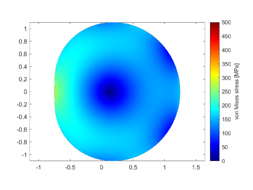
(a) $a=0.5$ and $c=10^{-3}$

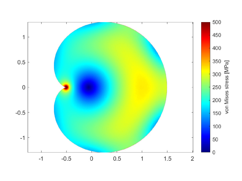
(b) $a=0.99$ and $c=10^{-3}$

Figure 1. Internal distribution of von Mises stress for different values of $a$

$\Box$

Example 5.2.

In this example, we shall consider an eccentric annulus. Let $\Omega_{b}$ be the image of the annulus $\mathbb{A}_{\frac{1}{2}}$ under the mapping $\varphi_{b}=\frac{z-b}{1-bz}$ where $0<b<1$. The new domain $\Omega_{b}$ is then defined as $\Omega_{b}=B(0,1)\setminus\overline{B(z_{b},r_{b})}$, with center $z_{b}=\frac{3b}{b^{2}-4}$ and radius $r_{b}=\frac{2(1-b^{2})}{4-b^{2}}$. Assume the potentials of the force acting on the domain are given by:

$$\phi(z) =-\frac{(2\mu+\lambda)}{\rho}c(x^{2}-y^{2})$$

$$\boldsymbol{A} =-\frac{2\mu}{\rho}xy,$$

which implies that $\psi=c\zeta^{2}$. Let us also consider the case when the complex traction potential is given by

$$\gamma(w)=\frac{c(1-b^{2})(w+b)}{|1+bw|^{2}(1+bw)}+\frac{c|w|^{2}(w+b)}{1+b\overline{w}}+\frac{cw^{2}(\overline{w}+b)}{2(1+bw)}.$$

It can then readily be shown that the conditions for solvability are satisfied and we obtain a canonical solution as:

$$v(z)=\frac{c}{2}\frac{(z-b)|z-b|^{2}}{(1-bz)|1-bz|^{2}}+c(z-b),$$

which yields to $v(b)=0$.

Setting $b=0.5$ and $c=10^{-3}$ gives us the internal distribution of von Mises stress as shown in Fig. 2.

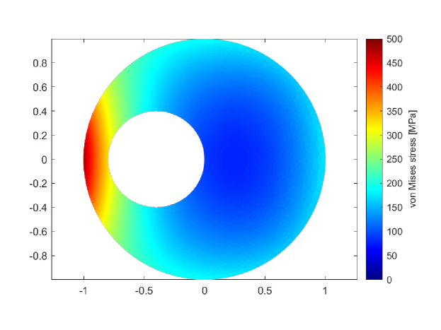
Figure 2. Internal distribution of von Mises stress due to a linear load with scaling constant $c=10^{-3}$.

$\Box$

Example 5.3.

Consider the gear-like domain $\Omega_{a}$, defined as the image of an annulus $\mathbb{A}_{r}$ with inner radius $r=1/2$ under the map $\varphi_{a}=\frac{a\zeta^{4}}{4}+\zeta$ with $0<a<1$. This domain represents a epitrochoid. We assume that the complex boundary traction potential, $\gamma_{a}(w)$, is given by the formula:

$$\gamma_{a}(w)=\\ \frac{2c\varphi_{a}^{-1}(w)+2c|w|^{2}\varphi_{a}^{-1}(w)(a(\varphi_{a}^{-1}(w))^{3}+1)+cw^{2}\overline{\varphi_{a}^{-1}(w)}(a\overline{(\varphi_{a}^{-1}(w))}^{3}+1)}{2|a(\varphi_{a}^{-1}(w))^{3}+1|},$$

where $\varphi_{a}^{-1}(w)$ is defined as:

$$\varphi_{a}^{-1}(w)=\frac{1}{2}\left(-\sqrt{Y(w)}+\sqrt{-2Y(w)+\frac{8}{a\sqrt{2Y(w)}}}\right),$$

and $Y(w)$ and $X(w)$ are given by:

$$Y(w)=X(w)-\frac{4w}{3aX(w)},\ \ X(w)=a^{-\frac{2}{3}}\root 3 \of{1+\sqrt{1+\frac{64aw^{3}}{27}}}.$$

We consider the action of a constant force, with potentials $\phi(z)$ and $\boldsymbol{A}$ defined as:

$$\phi(z) =-\frac{(2\mu+\lambda)}{\rho}c(x^{2}-y^{2}),$$

$$\boldsymbol{A} =-\frac{2\mu}{\rho}xy,$$

yielding $\psi=c\zeta^{2}$. The canonical solution is then given by:

$$v_{a}(z)=\frac{c}{2}\left|\frac{a}{4}z^{4}+z\right|^{2}\left(\frac{a}{4}z^{4}+z\right)+cz.$$

Here we face a situation similar to Application 5.1. The same reasoning applies, but we forego the details to avoid repetition and suggest revisiting Application 5.1 for understanding.

The resulting internal distribution of von Mises stress with $c=10^{-3}$ and the choices $a=0.5$ and $a=0.99$ are shown in Fig. 3.

(a) $a=0.5$ and $c=10^{-3}$

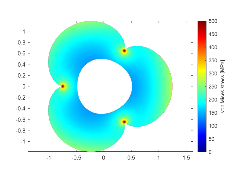
(b) $a=0.99$ and $c=10^{-3}$

Figure 3. Internal distribution of von Mises stress for different values of $a$

$\Box$

6. Conclusion

In this paper, we presented a methodology that seeks to address challenges in isotropic planar elastostatics based on the Neumann problem for the inhomogeneous Cauchy-Riemann problem. Our approach is tailored for domains conformally equivalent to the unit disk or an annulus.

Features of our method

• Direct Correspondence: Our method explores a connection between the plane elasticity problem described in (1.1) and the Neumann problem for the inhomogeneous Cauchy-Riemann problem domains.

• Flexibility and Scope: While many techniques are designed for specific force classes or domains, our method aims to provide a broader perspective by setting conditions on a wider range of domains and data smoothness criteria.

• Focus on the Displacement Field: Instead of prioritizing the stress tensor, which is common in many established methods, our approach attempts to provide an explicit formula for the displacement field.

• Simpler Approach: Avoiding the need for a rational conformal map, our methodology offers a wider perspective. This is further accentuated by minimizing intermediary constructs, which are prominent in methods such as the real integral equation and the Somigliana methods.

• Range of Applicability: Our method has been tested on a variety of domains, including cardioid structures and gear-like configurations, showcasing its potential applications.

In conclusion, our research introduces an approach that, while new, draws from existing concepts in isotropic planar elastostatics and offers potential avenues for broader applications.

Declaration of competing interest

The authors declare that they have no known competing financial interests or personal relationships that could have appeared to influence the work reported in this paper.

Data availability

No data was used for the research described in the article.

References

- [1] Alaci, S., Ciornei, F.-C., Romanu, I.-C.: Stress state in an eccentric elastic ring loaded symmetrically by concentrated forces. Mathematics (Basel) 10(8), 1314– (2022).
- [2] Alaci, S., Ciornei, F.-C., Filote, C.: Theoretical and experimental stress states in diametrically loaded eccentric rings. J. Balk. Tribol. Assoc. 22, 2959–2979 (2016).
- [3] Begehr, H.: Boundary value problems in complex analysis I. Boletín AMV 12(1), 65–86 (2005).
- [4] Busch, M., Heinzelmann, M., Maschke, H.G.: A cohesive zone model for the failure assessment of V-notches in micromechanical components. Int. J. Fract. 69(1), R15–R21 (1995).
- [5] Chen, J., Tsai, M.-H., Liu, C.-S.: Conformal mapping and bipolar coordinate for eccentric Laplace problems. Comput. Appl. Eng. Educ. 17(3), 314–322 (2009).
- [6] Chen, J., Shieh, H., Lee, Y.D., Lee, J.: Bipolar coordinates, image method and the method of fundamental solutions for Green’s functions of Laplace problems containing circular boundaries. Eng. Anal. Bound. Elem. 35(2), 236–243 (2011).
- [7] Constanda, C. The Boundary Integral Equation Method in Plane Elasticity. Proceedings of the American Mathematical Society. 123(11), pp.3385–3396 (1995).
- [8] Desai, P., Pandya, V.: Airy’s stress solution for isotropic rings with eccentric hole subjected to pressure. Int. J. Mech. Solids 12, 211–233 (2017).
- [9] England, A.H.: Complex variable methods in elasticity. Dover Publications, New York (2003).
- [10] Sen Gupta, A.M.: Stresses due to diametral forces on a circular disk with an eccentric hole. J. Appl. Mech. 22(2), 263–266 (1955).
- [11] Gupta, D.P.: Stresses due to diametral forces in tension on an eccentric hole of a circular disc. Z. Angew. Math. Mech. 40(5-6), 246–252 (1960).
- [12] Helsing, J., Jonsson, A.: On the computation of stress fields on polygonal domains with V-notches. Int. J. Numer. Methods Eng. 53(2), 433-453 (2002).
- [13] Inglis, C.E.: Stresses in a plate due to the presence of cracks and sharp corners. Trans. Inst. Naval Arch. 55, 219–230 (1913).
- [14] Kirsch, G.: Die Theorie der Elastizität und die Bedürfnisse der Festigkeitslehre. Zantralblatt Verlin Dtsch. Ing. 42, 797–807 (1898).
- [15] Kolosov, G.V.: On an application of complex function theory to a problem of the mathematical theory of elasticity. Doctoral Thesis, Yuryev (Tartu or Dorpat) University (1909).
- [16] Khomasuridze, N.: Solution of some elasticity boundary value problems in bipolar coordinates. Acta Mechanica 189(3-4), 207–224 (2007).
- [17] Leitman, M.J., Villaggio, P.: Some ambiguities in the complex variable method in elasticity. J. Elasticity 109(2), 223–234 (2012).
- [18] Leitman, M.J., Villaggio, P.: An extension of the complex variable method in plane elasticity to domains with corners: a notch problem. J. Elasticity 81(2), 205–215 (2005).
- [19] Lurie, A.I., Belyaev, A.: Theory of elasticity. Springer, Berlin Heidelberg (2005).
- [20] Muskhelishvili, N.: Some basic problems of the mathematical theory of elasticity. Springer, Netherlands (2013).
- [21] Neuber, H. Kerbspannungslehre. Springer, Berlin Heidelberg New York (1985).
- [22] Rizzo, F.J. An integral equation approach to boundary value problems of classical elastostatics. Quarterly of applied mathematics. 25(1), pp.83–95 (1967).
- [23] Solov’ev, I.I.: The action of a concentrated force on an eccentric ring. J. Appl. Math. Mech. 22(5), 989–996 (1958).
- [24] Vaitekhovich, T.S.: Boundary value problems to first-order complex partial differential equations in a ring domain. Integral Transforms Spec. Funct. 19(3), 211-233 (2008).
- [25] Westergaard, H.M.: Bearing pressures and cracks. J. Appl. Mech. 6, A49-A53 (1939).
- [26] Williams, M.L.: Stress singularities resulting from various boundary conditions in angular corners of plates in extension. J. Appl. Mech. 19(4), 526–528 (1952).
- [27] Yun, B.I.: An alternative complex variable method in plane elasticity. J. Korean Soc. Ind. Appl. Math. 65–74 (1997).