Solving a class of multi-scale elliptic PDEs by Fourier-based mixed physics informed neural networks

Abstract

Deep neural networks have garnered widespread attention due to their simplicity and flexibility in the fields of engineering and scientific calculation. In this study, we probe into solving a class of elliptic partial differential equations(PDEs) with multiple scales by utilizing Fourier-based mixed physics informed neural networks(dubbed FMPINN), its solver is configured as a multi-scale deep neural network. In contrast to the classical PINN method, a dual (flux) variable about the rough coefficient of PDEs is introduced to avoid the ill-condition of neural tangent kernel matrix caused by the oscillating coefficient of multi-scale PDEs. Therefore, apart from the physical conservation laws, the discrepancy between the auxiliary variables and the gradients of multi-scale coefficients is incorporated into the cost function, then obtaining a satisfactory solution of PDEs by minimizing the defined loss through some optimization methods. Additionally, a trigonometric activation function is introduced for FMPINN, which is suited for representing the derivatives of complex target functions. Handling the input data by Fourier feature mapping will effectively improve the capacity of deep neural networks to solve high-frequency problems. Finally, to validate the efficiency and robustness of the proposed FMPINN algorithm, we present several numerical examples of multi-scale problems in various dimensional Euclidean spaces. These examples cover both low-frequency and high-frequency oscillation cases, demonstrating the effectiveness of our approach. All code and data accompanying this manuscript will be made publicly available at https://github.com/Blue-Giant/FMPINN.

1 Introduction

Multi-scale problems, governed by partial differential equations(PDEs) with multiple scales, are prevalent in diverse scientific and engineering fields like reservoir simulation, high-frequency scattering, and turbulence modeling. This paper focuses on solving the following type of multi-scale problem.

$$\begin{cases}-\textbf{div}\bigg{(}A^{\varepsilon}(\bm{x})\nabla u^{\varepsilon}(\bm{x})\bigg{)}=f(\bm{x}),~{}~{}~{}\bm{x}\in\Omega,\\ ~{}~{}~{}~{}~{}~{}~{}~{}~{}~{}~{}\mathcal{B}u^{\varepsilon}(\bm{x})=g(\bm{x}),~{}~{}~{}~{}~{}~{}~{}~{}~{}~{}~{}~{}\bm{x}\in\partial\Omega.\end{cases}$$ (1.1)

where $\Omega$ is a bounded subset of $\mathbb{R}^{d}(d=1,2,3,\ldots)$ with piecewise Lipschitz boundary and satisfies the interior cone condition, $\varepsilon$ is a small positive parameter that signifies explicitly the multiscale nature of the rough coefficient $A^{\varepsilon}(\bm{x})$. $\mathcal{B}$ is a boundary operator in $\partial\Omega$ that imposes the boundary condition of $u^{\varepsilon}$, such as Dirchlete, Neumman and Robin. $\nabla$ and div are the gradient and divergence operators, respectively. $f(\bm{x})\in L^{2}(\Omega)$ is a given function. In addition, $A^{\varepsilon}(\bm{x})$ is symmetric and uniformly elliptic on $\Omega$. It means that all eigenvalues of $A^{\varepsilon}$ are uniformly bounded by two strictly positive constants $\lambda_{\min}(A^{\varepsilon})$ and $\lambda_{\max}(A^{\varepsilon})$. In other word, for all $\bm{x}\in\Omega$ and $\bm{\xi}\in\mathbb{R}^{d}$, we have

$$\lambda_{\min}(A^{\varepsilon})|\bm{\xi}|^{2}\leqslant\bm{\xi}^{T}A^{\varepsilon}(\bm{x})\bm{\xi}\leqslant\lambda_{\max}(A^{\varepsilon})|\bm{\xi}|^{2}.$$ (1.2)

The multi-scale problem(1.1) frequently arise in the fields of physical simulations and engineering applications, including the study of flow in porous media and the analysis of mechanical properties in composite materials [Ming2006, ming2005analysis, li2012efficient]. Generally, the analytical solutions of (1.1) are seldom available, then solving numerically this problem through approximation methods is necessary. Lots of numerical methods focus on efficient, accurate and stable numerical schemes have gained favorable achievement, such as heterogeneous multi-scale methods [ming2005analysis, li2012efficient, abdulle2014analysis], numerical homogenization [dur91, ab05, hellman2019numerical], variational multi-scale methods [hughes98, larson2007adaptive], multi-scale finite element methods [Arbogast_two_scale_04, eh09, ch03], flux norm homogenization [berlyand2010flux, owhadi2008homogenization], rough polyharmonic splines (RPS)[owhadi2014polyharmonic], generalized multi-scale finite element methods [Efendiev2013, chung2014adaptiveDG, chung2015residual], localized orthogonal decomposition [MalPet:2014, Henning2014], etc. In contrast to standard numerical methods including FEM and FDM, they alleviate substantially the computational complexity in handling all relevant scales, improve the numerical stabilities and expedite the convergence. However, they still will encounter the curse of complex domain and dimensionality in general.

Deep neural networks(DNN), an efficient meshfree method without the discretization for a given interested domain, have drawn more and more attention from researchers to solve numerically the ordinary and partial differential equations as well as the inverse problems for complex geometrical domain and high-dimensional cases [e2018the, sirignano2018dgm, chen2018neural, raissi2019physics, khoo2019switchnet, zang2020weak, lyu2022mim], due to their extraordinary universal approximation capacity[hauptmann2020deep]. Among these methods, the physics-informed neural networks (PINN) dating back to the early 1990s again attracted widespread attention of researchers and have made remarkable achievements for approximating the solution of PDEs by embracing the physical laws with neural networks, on account of the rapid development of computer science and technology[raissi2019physics, dissanayake1994neural]. This method skillfully incorporates the residual of governing equations and the discrepancy of boundary/initial constraints, then formulates a cost function can be optimized easily via the automatic differentiation in DNN. Many efforts have been made to further enhance the performance of PINN are concluded as two aspects: refining the selection of the residual term and designing the manner of initial/boundary constraints. In terms of the residual term, there are XPINN [jagtap2021extended], cPINN [jagtap2020conservative], two-stage PINN [lin2022two] and gPINN [yu2022gradient], and so on. By subtly encoding the I/B constraints into DNN in a hard manner, the PINN can be easy to train with low computational complexity and obtain a high-precision solution of PDEs with complex boundary conditions[berg2018a, sun2020surrogate, lu2021physics]. Motivated by the reduction of order in conventional methods[ch03], some attempts have been made to solve the high-order PDEs by reframing them as some first-order systems, this will overcome the shortcomings of the computational burden for high-order derivatives in DNN. For example, the deep mixed residual method [lyu2022mim], the local deep learning method[zhu2021local] and the deep FOSLS method[cai2020deep, bersetche2023deep].

Many studies and experiments have indicated that the general DNN-based algorithms are commonly used to solve a low-frequency problem in varying dimensional space, but will encounter tremendous challenge for high-frequency problems such as multi-scale PDEs(1.1). The frequency principle[Xu_2020] or spectral bias[rahaman2018spectral] of DNN shows that neural networks are typically efficient for fitting objective functions with low-frequency modes but inefficient for high-frequency functions. Then, a series of multi-scale DNN(MscaleDNN) algorithms were proposed to overcome the shortcomings of normal DNN for high-frequency problems by converting high-frequency contents into low-frequency ones via a radial scale technique [liu2020multi, wang2020multiscale, li2020elliptic, li2023subspace]. After that, some corresponding mechanisms were developed to explain this performance of DNN, such as the Neural Tangent Kernel (NTK)[wang2020eigenvector, jacot2018neural]. Furthermore, many researchers attempted to utilize a Fourier feature mapping consisting of sine and cosine to improve the capacity of MscaleDNN, which will alleviate the pathology of spectral bias and let neural networks capture high frequencies component effectively[wang2020eigenvector, ramabathiran2021spinn, li2023subspace, li2023deep, tancik2020fourier, han2021hierarchical].

Recently, some works[leung2022nh, carney2022physics] have shown that general PINN architecture is unable to capture the multi-scale property of the solution due to the effect of rough coefficient in multi-scale PDEs. In [leung2022nh], Wing Tat Leung et.al proposed a Neural homogenization-based PINN(NH-PINN) method to solve (1.1), it can well overcome the unconvergence of PINN for multi-scale problems. However, NH-PINN also will encounter the dilemma of dimensional and the burden of computation, because it will convert one low-dimensional problem into a high-dimensional case. By carefully analyzing the Neural Tangent Kernel matrix associated with the PINN, Sean P. Carney et. al[carney2022physics] found that the Forbenius norm of the NTK matrix will become unbound as the oscillation factor $\varepsilon$ in $A^{\varepsilon}$ tends to zero. It means that the evolution of residual loss term in PINN will become increasingly stiff as $\varepsilon\rightarrow 0$, then lead to poor training behavior for PINN.

In this paper, a Fourier-based multi-scale mixed PINN(FMPINN) structure is proposed to solve the multi-scale problems (1.1) with rough coefficients. This method consists of the general PINN architecture and the aforementioned MscaleDNN model with subnetworks being used to capture different frequencies component. To overcome the weakness of the normal PINN that failed to capture the jumping gradient information of the oscillating coefficient when tackling the governed equation in multi-scale PDEs(1.1), a (dual)flux variable is introduced to alleviate the adverse effect of the rough coefficient. Meantime, it can also reduce the computational burden of PINN for the second-order derivatives of space variables. In addition, the Fourier feature mapping is used in our model to learn each target frequency efficiently and express the derivatives of multi-frequency functions easily, it will remarkably improve the capacity for our FMPINN model to solve multi-scale problems. In a nutshell, the primary contributions of this paper are summarized as follows:

1. We propose a novel neural networks approach by combining normal PINN and MscaleDNN with subnetworks structure to address multi-scale problems, leveraging the Fourier theorem and the F-principle of DNN.

2. Inspired by the reduced order scheme for high-order PDEs, a dual (flux) variable about the rough coefficient of multi-scale PDEs is introduced to address the gradient leakage about the rough coefficient for PINN.

3. By introducing some numerical experiments, we show that the classical PINN method with MscaleDNN solver is still insufficient in providing accurate solutions for multi-scale equations.

4. We showcase the exceptional performance of FMPINN in solving a class of multi-scale elliptic PDEs with essential boundaries in various dimensional spaces. Our method outperforms existing approaches and demonstrates its superiority in addressing these complex problems.

The remaining parts of our work are organized as follows. In Section 2, we briefly introduce the underlying conceptions and formulations for MscaleDNN and the structure of PINN. Section 3 provides a unified architecture of the FMPINN to solve the elliptic multi-scale problem (1.1) based on its equivalent reduced order scheme, and gives the option of activation function as well as the error analysis of our proppsed method. Section 4 details the FMPINN algorithm for approximating the solution of multi-scale PDEs, then provide the option of activation function and the simple error analysis for FMPINN method. In Section LABEL:sec:04, some scenarios of multi-scale PDEs are performed to evaluate the feasibility and effectiveness of our proposed method. Finally, some conclusions of this paper are made in Section LABEL:sec:05.

2 Multi-scale Physics Informed Neural Networks

2.1 Multi-scale Deep Neural Networks with ResNet technique

The basic concept and formulation of DNN are described briefly in this section, which helps audiences to understand the DNN structure through functional terminology. Mathematically, a deep neural network defines the following mapping

$$\mathcal{F}:\bm{x}\in\mathbb{R}^{d}\Longrightarrow\bm{y}=\mathcal{F}(x)\in\mathbb{R}^{c}$$ (2.1)

with $d$ and $c$ being the dimensions of input and output, respectively. In fact, the DNN functional $\mathcal{F}$ is a nested composition of the following single-layer neural unit:

$$\bm{y}=\{y_{1},y_{2},\cdots,y_{m}\}~{}~{}\textup{and}~{}~{}y_{l}=\sigma\left(\sum_{n=1}^{d}w_{ln}*x_{n}+b_{l}\right)$$ (2.2)

where $w_{ln}$ and $b_{l}$ are called weight and bias of $l_{th}$ neuron, respectively. $\sigma(\cdot)$ is an element-wise non-linear operator, generally referred as the activation function. Then, we have the following formulation of DNN:

$$\bm{y}^{[\ell]}=\sigma\circ(\bm{W}^{[\ell]}\bm{y}^{[\ell-1]}+\bm{b}^{[\ell]}),~{}~{}\text{for}~{}~{}\ell=1,2,3,\cdots\cdots,L$$ (2.3)

and $\bm{y}^{[0]}=\bm{x}$, where $\bm{W}^{[\ell]}\in\mathbb{R}^{n_{\ell+1}\times n_{\ell}},\bm{b}^{[\ell]}\in\mathbb{R}^{n_{\ell+1}}$ stand for the weight matrix and bias vector of $\ell$-th hidden layer, respectively, $n_{0}=d$ and $n_{L+1}$ is the dimension of output, and $``\circ"$ stands for the elementary-wise operation. For convenience, the output of DNN is denoted by $\bm{y}(\bm{x};\bm{\theta})$ with $\bm{\theta}$ standing for its all weights and biases.

Residual neural network (ResNet) [he2016deep] as a common skillful technique by introducing skip connections between adjacent or nonadjacent hidden layers can overcome effectively the vanishing gradient of parameters in the backpropagation for DNN, then make the network much easier to train and improve well the performance of DNN. Many experiment results showed that the ResNet can also improve the performance of DNNs to approximate high-order derivatives and solutions of PDEs [e2018the, lyu2022mim]. We utilize the one-step skip connection scheme of ResNet in this work. Except for the normal data flow, the data will also flow along with the skip connection if the two consecutive layers in DNN have the same number of neurons, otherwise, the data flows directly from one to the next layer. The filtered $\bm{y}^{[\ell+1]}(\bm{x};\bm{\theta})$ produced by the input $\bm{y}^{[\ell]}(\bm{x};\bm{\theta})$ is expressed as

$$\bm{y}^{[\ell+1]}(\bm{x};\bm{\theta})=\bm{y}^{[\ell]}(\bm{x};\bm{\theta})+\sigma\circ\bigg{(}\bm{W}^{[\ell+1]}\bm{y}^{[\ell]}(\bm{x};\bm{\theta})+\bm{b}^{[\ell+1]}\bigg{)}.$$

As we are aware, a normal DNN model is capable of providing a satisfactory solution for general problems. However, it will encounter troublesome difficulty to solve multi-scale problems with high-frequency components. Recently, a MscaleDNN architecture has shown its remarkable performance to deal with high-frequency problems by converting original data to a low-frequency space [liu2020multi, wang2020multiscale, li2020elliptic, wang2020eigenvector]. A schematic diagram of MscaleDNN with $Q$ subnetworks is depicted in Fig. 1.

Figure 1: A schematic diagram of MscaleDNN with $Q$ subnetworks, $\sigma$ stands for the activation function

The detailed procedure of MscaleDNN is described in the following.

1. Generating a scale vector or matrix with $Q$ parts

   $$\Lambda=(\bm{k}_{1},\bm{k}_{2},\bm{k}_{3}\cdots,\bm{k}_{Q-1},\bm{k}_{Q})^{T},$$ (2.4)

   where $\bm{k}_{i}(i=1,2,\ldots,Q)$ is a scalar or matrix (trainable or untrainable).

2. Converting the input data $\bm{x}$ into $\tilde{\bm{x}}=\Lambda\odot\bm{x}$ with $\odot$ being the Hadamard product, then feeding $\tilde{\bm{x}}$ into the pipeline of MscaleDNN. It is

   $$\begin{cases}\hat{\bm{x}}=\bm{k}_{i}\bm{x}\\ \bm{F}_{i}(\bm{x})=\mathcal{FCN}_{i}\left(\hat{\bm{x}}\right)\end{cases}\quad i=1,2,\ldots,Q,$$ (2.5)

   where $\mathcal{FCN}_{i}$ stands for the $i_{th}$ fully connected subnetwork and $\bm{F}_{i}$ is its output.

3. Obtaining the result of MscaleDNN by aggregating linearly the output of all subnetworks, each scale input goes through a subnetwork. It is

   $$\bm{NN}(\bm{x})=\bm{W}_{O}\cdot\left[\bm{F}_{1}(\bm{x}),\bm{F}_{2}(\bm{x}),\cdots,\bm{F}_{Q}(\bm{x})\right]+\bm{b}_{O},$$ (2.6)

   where $\bm{W}_{O}$ and $\bm{b}_{O}$ stand for the weights and biases of the last linear layer, respectively.

From the perspective of Fourier transformation and decomposition, the first layer of the MscaleDNN model will be treated as a series of basis in Fourier space and its output is the combination of basis functions [liu2020multi, li2020elliptic, wang2020eigenvector].

2.2 Overview of Physics-Informed Neural Networks

In the scope of PINN, a type of PDE governed by parameters as the toy to show its implementation, it is

$$\mathcal{N}_{\bm{\lambda}}[\hat{u}(\bm{x})]=\hat{f}(\bm{x}),\quad\bm{x}\in\Omega$$ (2.7)

$$\mathcal{B}\hat{u}\left(\bm{x}\right)=\hat{g}(\bm{x}),\quad\quad\bm{x}\in\partial\Omega$$

in which $\mathcal{N}_{\bm{\lambda}}$ stands for the linear or nonlinear differential operator with parameters $\bm{\lambda}$, $\mathcal{B}$ is the boundary operator, such as Dirichlet, Neumann, periodic boundary conditions, or a mixed form of them. $\Omega$ and $\partial\Omega$ respectively illustrate the zone of interest and its border. For approximating the solution of the multi-scale PDE, a multi-scale deep neural network is used. In classical PINN, the ideal parameters of the DNN can be obtained by minimizing the following composite loss function

$$Loss=Loss_{R}+\gamma Loss_{B}$$ (2.8)

with

$$Loss_{R}=\frac{1}{N_{R}}\sum_{i=1}^{N_{R}}\left\|\mathcal{N}_{\bm{\lambda}}[u_{NN}(\bm{x}^{i}_{I})]-\hat{f}(\bm{x}^{i}_{I})\right\|^{2}$$ (2.9)

$$Loss_{B}=\frac{1}{N_{B}}\sum_{j=1}^{N_{B}}\bigg{\|}\mathcal{B}u_{NN}\left(\bm{x}^{j}_{B}\right)-\hat{g}(\bm{x}^{j}_{B})\bigg{\|}^{2}$$

where $\gamma>0$ is used to control the contribution for the corresponding loss term. $Loss_{R}$ and $Loss_{B}$ depict the residual of the governing equations and the loss on the boundary condition, respectively. If some additional observed data are available inside the interested domain, then a loss term indicating the mismatch between the predictions produced by DNN and the observations can be taken into account

$$Loss_{D}=\frac{1}{N_{D}}\sum_{i=1}^{N_{D}}\bigg{\|}u_{NN}(\bm{x}^{i})-u_{Data}^{i}\bigg{\|}^{2}.$$ (2.10)

3 Fourier-based mixed PINN to solve multi-scale problem

In this section, the unified architecture of FMPINN is proposed to overcome the adverse effect of derivative for rough coefficient $A^{\varepsilon}$ by embracing a multi-output neural network with an equivalent reduced-order formulation of the multi-scale problem (1.1).

3.1 Failure of classical PINN

Despite the success of various PINN models in studying ordinary and partial differential equations, it has been observed in [leung2022nh] that the classical PINN approach fails to provide accurate predictions for multi-scale PDEs(1.1). Furthermore, we find that a direct application of the PINN with multi-scale DNN framework on solving (1.1) still cannot provide a satisfactory solution, because of the ill-posed NTK matrix caused by rough coefficient $A^{\varepsilon}$. For example, let us consider the following one-dimensional elliptic equation with a homogeneous Dirichlet boundary in $\Omega=[0,1]$:

$$\begin{cases}\displaystyle-\frac{d}{dx}\bigg{(}A^{\varepsilon}(x)\frac{d}{dx}u^{\varepsilon}(x)\bigg{)}=5\cos(\pi x)\\ ~{}~{}~{}~{}~{}~{}~{}~{}~{}~{}~{}u^{\varepsilon}(0)=u^{\varepsilon}(1)=0\end{cases},$$

in which $\displaystyle A^{\varepsilon}(x)=\frac{1+x^{2}}{2+\sin(2\pi x/\varepsilon)}$ with $\varepsilon>0$ being a small constant.

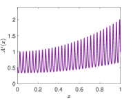
(a) $A^{\varepsilon}$ for $\varepsilon=1/32$

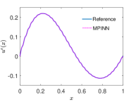
(b) $u^{\varepsilon}$ for $\varepsilon=1/32$

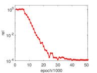
(c) $l^{2}$ relative error for $\varepsilon=1/32$

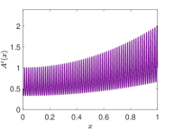
(d) $A^{\varepsilon}$ for $\varepsilon=1/64$

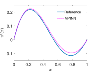
(e) $u^{\varepsilon}$ for $\varepsilon=1/64$

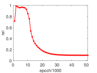
(f) $l^{2}$ relative error for $\varepsilon=1/64$

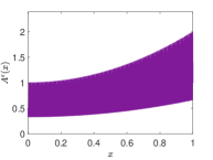
(g) $A^{\varepsilon}$ for $\varepsilon=1/128$

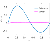
(h) $u^{\varepsilon}$ for $\varepsilon=1/128$

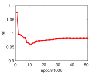
(i) $l^{2}$ relative error for $\varepsilon=1/128$

Figure 2: Left: the rough coefficient $A^{\varepsilon}$. Middle: the MPINN approximated solution vs the reference solution. Right: $l^{2}$ relative error varies with the testing epoch.

We employ the classical PINN method with the MscaleDNN framework(see Fig. 1) to solve (1.1), called this method as MPINN. The scale factors $\Lambda$ for MscaleDNN is set as $(1,2,3,4,5,10,\cdots,90,95,100)$ and the size of each subnetwork is chosen as $(1,30,40,30,30,30,1)$. The activation function of the first hidden layer for all subnetworks is set as Fourier feature mapping(see Section 3.3) and the other activation functions(except for their output layer) are chosen as $\frac{1}{2}\sin(x)+\frac{1}{2}\cos(x)$ [chen2022adaptive], their output layers are all linear. For $\varepsilon=\frac{1}{32},\frac{1}{64}$ and $\frac{1}{128}$,We train the aforementioned MPINN model for 50000 epochs and conduct testing every 1000 epochs within the training cycle. The optimizer is set as Adam with an initial learning rate of 0.01 and the learning rate will decay by $2.5\%$ for every 100 epochs. Finally, the results are demonstrated in Fig. 2.

As $\varepsilon=1/32$, the coefficient $A^{\varepsilon}(x)$ possesses a little multi-scale information, the MPINN performs quite well. However, the permeability $A^{\varepsilon}(x)$ will exhibits various multi-scale properties for $\varepsilon=1/64$, the performance of MPINN deteriorates with a low relative error and the MPINN fails to converge for $\varepsilon=1/128$. In addition, we perform the MPINN with different setups of the hyperparameters such as the learning rate and the $\omega_{B}$ for $Loss_{B}$ in (2.8) as well as the network size, but we still cannot obtain a satisfactory result.

3.2 Unified architecture of FMPINN

Based on the above observation, it is necessary to seek some extra techniques to improve the accuracy of the PINN. Inspired by the mixed finite element method [ch03, araya2013multiscale] and the mixed residual method[lyu2022mim], we can leverage a mixed scheme to solve (1.1) by replacing the flux term $A^{\varepsilon}\nabla u$ in (1.1) with an auxiliary variable. This strategy not only can avoid the unfavorable effect of the oscillating coefficient $A^{\varepsilon}$, but also can reduce the computation burden of second-order derivatives in cost function when utilizing a multi-scale deep neural network to approximate the solution of (1.1). Therefore, we introduce a flux variable $\bm{\phi}(\bm{x})=\big{(}\phi_{1}(\bm{x}),\ldots,\phi_{d}(\bm{x})\big{)}=A^{\varepsilon}(\bm{x})\nabla u^{\varepsilon}(\bm{x})$ and rewrite the first equation in (1.1) as the following expressions:

$$-\mathbf{div}\bm{\phi}(\bm{x})=f(\bm{x})$$ (3.1)

$$\bm{\phi}(\bm{x})-A^{\varepsilon}(\bm{x})\nabla u^{\varepsilon}(\bm{x})=\bm{0}$$

Then we turn to search a couple of functions $(u^{\varepsilon},\bm{\phi})$ in admissible space, rather than approximating a unique solution of the original problem (1.1). Here and thereafter, $(u^{\varepsilon},\bm{\phi})\in\mathcal{A}=\mathcal{H}^{1}(\Omega)\times\mathcal{H}(\mathbf{div};\Omega)$ with $\mathcal{H}^{1}(\Omega)=\big{\{}v\in L^{2}(\Omega):\nabla v\in L^{2}(\Omega)\big{\}}$ and $\mathcal{H}(\mathbf{div};\Omega)=\big{\{}\bm{\psi}\in[L^{2}(\Omega)]^{d}:\mathbf{div}\bm{\psi}\in L^{2}(\Omega)\big{\}}.$

When utilizing numerical solvers to address the equation (3.1), one can obtain the optimum solution by minimizing the following least-squares formula in the domain $\Omega$:

$$u^{*},\bm{\phi}^{*}=\underset{(u,\bm{\phi})\in\mathcal{H}^{1}(\Omega)\times\mathcal{H}(\mathbf{div};\Omega)}{\arg\min}\mathcal{L}(u,\bm{\phi})$$ (3.2)

with

$$\mathcal{L}(u,\bm{\phi})=\int_{\Omega}\big{|}-\mathbf{div}\bm{\phi}(\bm{x})-f(\bm{x})\big{|}^{2}d\bm{x}+\beta\int_{\Omega}\big{|}\bm{\phi}(\bm{x})-A^{\varepsilon}(\bm{x})\nabla u^{\varepsilon}(\bm{x})\big{|}^{2}d\bm{x}$$ (3.3)

where $\beta>0$ is used to adjust the approximation error of the flux variable and flux term.

Generally, two independent neural networks are necessary to approximate the flux variable $\bm{\phi}$ and solution $u$, but $\bm{\phi}$ is unconstrained without any coercive boundary condition. Based on the potentiality of DNN for approximating any linear and non-linear complex functions, we take a DNN with multi outputs to model ansatzes $\bm{\phi}$ and $u$, denoted by $\bm{\phi}_{NN}$ and $u_{NN}$, respectively. Fig. 3 describes the multi-output neural network for input $\bm{x}\in\mathbb{R}^{2}$.

Figure 3: The multi-output neural network for approximating the state and flux variables

Once the expressions of auxiliary functions $\bm{\phi}$ and solution $u$ have been determined, we can discretize (3.3) by the Monte Carlo method [robert1999monte], then employ the PINN conception and obtain the following form

$$\mathscr{L}_{in}(S_{I};\bm{\theta})=\frac{|\Omega|}{N_{in}}\sum_{i=1}^{N_{in}}\bigg{[}\big{|}-\textbf{div}\bm{\phi}_{NN}(\bm{x}_{I}^{i};\bm{\theta})-f(\bm{x}_{I}^{i})\big{|}^{2}+\beta\big{|}\bm{\phi}_{NN}(\bm{x}^{i}_{I},\bm{\theta})-A^{\varepsilon}(\bm{x}^{i}_{I})\nabla u_{NN}(\bm{x}_{I}^{i},\bm{\theta})\big{|}^{2}\bigg{]},$$ (3.4)

for $\bm{x}_{I}^{i}\in S_{I}$, here and hereinafter $S_{I}$ stands for the collection sampled from $\Omega$ with prescribed probability density.

Same to the traditional numerical methods such as FDM and FEM for addressing PDEs, boundary conditions play a crucial role in DNN representation as well. They serve as important constraints that ensure the uniqueness and accuracy of the solution. Consequently, the output $u_{NN}$ of DNN should also satisfy the boundary conditions of (1.1), which means

$$\mathscr{L}_{bd}(S_{B};\bm{\theta})=\frac{1}{N_{bd}}\sum_{j=1}^{N_{bd}}\bigg{[}\mathcal{B}u_{NN}\big{(}\bm{x}_{B}^{j};\bm{\theta}\big{)}-g(\bm{x}_{B}^{j})\bigg{]}^{2}\rightarrow 0~{}~{}\text{for}~{}~{}\bm{x}_{B}^{j}\in S_{B}.$$ (3.5)

here and hereinafter $S_{B}$ represents the collection sampled on $\partial\Omega$ with prescribed probability density.

According to the above results, the weights and biases of the DNN model are updated by optimizing gradually the following cost function:

$$\mathscr{L}({S_{I},S_{B}};\bm{\theta})=\mathscr{L}_{in}(S_{I};\bm{\theta})+\gamma\mathscr{L}_{bd}(S_{B};\bm{\theta})$$ (3.6)

where $S_{I}=\{\bm{x}_{I}^{i}\}_{i=1}^{N_{in}}$ and $S_{B}=\{\bm{x}_{B}^{j}\}_{j=1}^{N_{bd}}$ stand for the train data of $\Omega$ and $\partial\Omega$, respectively. The term of $\mathscr{L}_{in}$ composed of the residual governed by differential equations and the discrepancy with respect to flux, minimizes the residual of the PDE, whereas the term of $\mathscr{L}_{bd}$ pushes the DNN solver to match the given boundary conditions. In addition, a constant parameter $\gamma>0$ is introduced to forces well the $\mathscr{L}_{bd}(S_{B};\bm{\theta})\rightarrow 0$ in the loss function, it is increasing gradually with training process going on.

Based on the analysis in [bersetche2023deep], a nonconstant continuous activation function $\sigma$ can guarantee the mapping $\bm{\theta}\mapsto(u_{NN},\bm{\phi}_{NN})$ is continuous, then the distance between approximation functions $\bm{q}_{NN}=(u_{NN},\bm{\phi}_{NN})$ and exact solution $\bm{q}^{*}=(u^{*},\bm{\phi}^{*})$ will decrease by adjusting gradually the parameters of DNN, i.e.,

$$d(\bm{q}^{*},\mathcal{A}_{k})=\underset{\bm{q}_{NN}\in\mathcal{A}_{k}}{\inf}\|\bm{q}^{*}-\bm{q}_{NN}\|\rightarrow 0~{}~{}\text{as}~{}~{}k\rightarrow\infty.$$

It means the loss function $\mathscr{L}({S_{I},S_{B}};\bm{\theta})$ will attain the corresponding minimum when $d\rightarrow 0$.

Hence, Our purpose is to find an optimal set of parameter $\bm{\theta}^{*}$ such that the approximations $u_{NN}$ and $\bm{\phi}_{NN}$ minimize the loss function $\mathscr{L}({S_{I},S_{B}};\bm{\theta})$. In order to obtain the ideal $\bm{\theta}^{*}$, one can update the weights and biases of DNN through the optimization methods such as gradient descent (GD) or stochastic gradient descent (SGD) during the training process. In this context, the SGD method with a ”mini-batch” of training data is given by:

$$\bm{\theta}^{k+1}=\bm{\theta}^{k}-\alpha^{k}\nabla_{\bm{\theta}^{k}}\mathscr{L}(\bm{x};\bm{\theta}^{k})~{}~{}\text{with}~{}~{}\bm{x}\in S_{I}~{}\text{or}~{}\bm{x}\in S_{B}$$ (3.7)

where the “learning rate” $\alpha^{k}$ decreases with $k$ increasing.

3.3 Option of activation function for FMPINN and its explanation

Choosing a suitable and effective activation function is a critical concern when aiming to enhance the performance of DNN in computer vision, natural language processing, and scientific computation. Generally, an activation function such as rectified linear unit $\text{ReLU}(\bm{z})$ and hyperbolic tangent function $\tanh(\bm{z})$, can obviously improve the capacity and nonlinearity of neural networkS to address various nonlinear problems, such as the solution of various PDEs and classification. Recently, the works [Xu_2020, rahaman2018spectral] manifested that the DNN often captures firstly the low-frequency component for target functions, then match the high-frequency component, they called it as the spectral bias or frequency preference of DNN. Under this phenomenon, many researchers attempt to utilize a Fourier feature mapping consisting of sine and cosine as the activation function to improve the capacity of MscaleDNN, it will mitigate the pathology of spectral bias and enable networks to learn high frequencies more effectively[rahaman2018spectral, wang2020eigenvector, tancik2020fourier, li2023deep]. It is expressed as follows:

$$\zeta(\bm{x})=\left[\begin{array}[]{c}\cos(\bm{\kappa}\bm{x})\\ \sin(\bm{\kappa}\bm{x})\end{array}\right],$$ (3.8)

where $\bm{\kappa}$ is a user-specified vector or matrix (trainable or untrainable) which is consistent with the number of neural units in the first hidden layer for DNNs. Further, the work [li2023subspace] designed a soften Fourier mapping by introducing a relaxing parameter $s\in(0,1]$ in $\zeta(\bm{x})$, numerical results show that this modification will improve the performance of $\zeta(\bm{x})$. Actually, this activation function is used in the first hidden layer of DNN and maps the input data in $\Omega$ into a range of $[-1,1]$, then enhances the ability of DNN and expedites its convergence.

Therefore, a real function $\mathcal{P}(x)$ represented by DNN can be expressed as follows

$$\mathcal{P}(\bm{x})=\sum_{n=0}^{\tilde{N}}\bigg{(}S\left(\cos(\bm{k}_{n}\bm{x});\bm{\bar{\theta}}_{n}\right)+T\left(\sin(\bm{k}_{n}\bm{x});\bm{\tilde{\theta}}_{n}\right)\bigg{)},$$

where $S(\cdot,\bm{\bar{\theta}}),T(\cdot,\bm{\tilde{\theta}})$ are the DNNs or the sub-modules of DNNs, respectively, $\{\bm{k}_{0},\bm{k}_{1},\bm{k}_{2},\cdots\}$ are the frequencies of interest for the objective function. Obviously, the first hidden layer performed by Fourier feature mapping mimics the Fourier basis function, and the remaining blocks with different activation functions are used to learn the coefficients of these functions. After performing the Fourier mapping for input points with a given scale factor, the neural network can well capture the fine varying information for multi-scale problems.

Remark 1.

(Lipschitz continuous) If an activation function $\sigma$ is continuous(i.e., $\sigma\in C^{1}$) and satisfies the following boundedness condition:

$$|\sigma(x)|<1~{}~{}~{}~{}\textup{and}~{}~{}~{}~{}|\sigma^{\prime}(x)|<1$$

for any $x\in\mathbb{R}$. Then, we have

$$|\sigma(x)-\sigma(y)|\leqslant|x-y|~{}~{}~{}~{}\textup{and}~{}~{}~{}~{}|\sigma^{\prime}(x)-\sigma^{\prime}(y)|<|x-y|$$

for any $x,y\in\mathbb{R}$. Obviously, the activation functions $\tanh(x)$, sigmoid(x), Fourier feature mapping $\zeta(a)$ and $\frac{1}{2}sin(x)+\frac{1}{2}cos(x)$ are all satisfy the above condition and have a good regularity, they will overcome the gradient explosion of parameter in the backpropagation for DNN and improve the capacity of DNN.

3.4 Simple error analysis for FMPINN

In recent times, there have been endeavors to rigorously analyze the convergence rate of the deep mixed residual method and compare it with the deep Galerkin method (DGM) and deep Ritz method (DRM) across different scenarios[bersetche2023deep, gu2023error, li2022priori]. In this study, we investigate those results of convergence again, then provide the expression of generalization error for FMPINN and some remarks of errors.

Figure 4: Illustration of the total error for FMPINN.

For convenience, let $\bm{q}^{*}=(u^{*},\bm{\phi}^{*})$ be the exact solution of equation (3.1) or the minimum of cost function (3.2) with (3.3) for coercive boundary constraints. Meantime, the $\bm{q}_{\bm{\theta}^{*}}=(u_{\bm{\theta}^{*}},\bm{\phi}_{\bm{\theta}^{*}})$ stands for the final output of DNN optimized by SGD optimizer(such as Adam or LBFGS) that attains the local minimum of (3.6). Further, we let $\widetilde{\mathscr{L}}(u,\bm{\phi})$ be the cost function evaluated on $N$ points sampled from $\Omega$ and denote the output of DNN as $\bm{q}_{\bm{\theta}}=(u_{\bm{\theta}},\bm{\phi}_{\bm{\theta}})$. Finally, $\mathcal{S}_{NN}$ represents the function space sapnned by the output of DNN. Then, the total error(or generalization error) between the exact solution $\bm{q}^{*}$ and the output of DNN $\bm{q}_{\bm{\theta}}$ can be expressed as

$$\big{\|}u_{\bm{\theta}}-u^{*}\big{\|}_{\mathcal{H}^{1}(\Omega)}+\big{\|}\bm{\phi}_{\bm{\theta}}-\bm{\phi}^{*}\big{\|}_{\mathcal{H}^{1}(\bm{div},\Omega)}\leqslant C(coe)\sqrt{\delta_{app}+\delta_{est}+\delta_{opt}}$$ (3.9)

with

$$\begin{cases}\delta_{app}=\underset{(u,\bm{\phi})\in\mathcal{S}_{NN}}{\inf}\|u-u^{*}\|^{2}_{\mathcal{H}^{1}(\Omega)}+\|\bm{\phi}-\bm{\phi}^{*}\|^{2}_{\mathcal{H}(\bm{div},\Omega)}\\ \delta_{est}=\underset{(u,\bm{\phi})\in\mathcal{S}_{NN}}{\sup}[\mathcal{L}(u,\bm{\phi})-\widetilde{\mathscr{L}}(u,\bm{\phi})]+\underset{(u,\bm{\phi})\in\mathcal{S}_{NN}}{\sup}[\widetilde{\mathscr{L}}(u,\bm{\phi})-\mathcal{L}(u,\bm{\phi})]\\ \delta_{opt}=\widetilde{\mathscr{L}}(u_{\bm{\theta}^{*}},\bm{\phi}_{\bm{\theta}^{*}})-\widetilde{\mathscr{L}}(u_{\bm{\theta}},\bm{\phi}_{\bm{\theta}})\end{cases}$$

In which, the approximated error $\delta_{app}$ indicates the difference between $(u^{*},\bm{\phi}^{*})$ and its projection onto $\mathcal{S}_{NN}$, the estimation error $\delta_{est}$ measures the difference between the continuous cost function $\mathcal{L}$ and discrete cost function $\widetilde{\mathscr{L}}$, the optimization error $\delta_{opt}$ stands for the discrepancy between the output of DNN with optimizing and the output of DNN without optimizing. In Fig. 4, we depict the diagram of error for FMPINN.

Remark 2.

For the approximating error, it is generally dependent on the architectural design of the neural network and the choice of the activation function. Classical radial basis network[orr1996introduction], the vanilla DNN and extreme learning machine(ELM)[ding2014extreme] are the common meshless method for approximating the solution of PDEs. To address the spatio-temporal problems, some hybrid network frameworks have been designed by combining PINN with traditional numerical methods to solve PDE, such as FDM-PINN and Runge-Kutta PINN[raissi2019physics, xiang2022hybrid]. Moreover, instead of soft constraints by a hard manner for the boundary or initial conditions in those methods, the approximation will automatically meet the boundary and initial conditions of PDEs, then reduce the complexity and improve the precision of NN[sun2020surrogate]. On the other hand, a powerful activation function, such as the hyperbolic tangent activation function and Fourier feature mapping, not only enhance the nonlinearity of DNN, but also improve its approximating capacity and accuracy. In addition, some available data are generally considered as a loss term to reduce the approximating error.

Remark 3.

Generally, the proposed FMPINN surrogate can provide more accurate approximations as the number of random collocation points increases. However, it will lead to heavy computational costs for lots of samplings. Then, it is worthwhile to take into account the trade-off between accuracy and computational cost when designing a DNN surrogate and determining its training mode. Alternatively, one can employ some effective low-discrepancy sampling approaches to decrease the statistical error, such as the Latin hypercube sampling method[viana2016tutorial], quasi-random sampling[shaw1988quasirandom] and multilevel Monte Carlo method[giles2015multilevel].

Remark 4.

Since the cost function generally is non-convex and has several local minima, then the gradient-based optimizer will almost certainly become caught in one of them. Therefore, choosing a good optimizer is important to reduce the optimization error and get a better minimum. In many scenarios of optimizing DNN, the Adam optimization method has shown its good performance including efficiency and accuracy, it can dynamically adjust the learning rates of each parameter by using the first and second moments estimation of the gradients[kingma2015adam]. BFGS is a quasi-Newton method and numerically stable, it may provide a higher-precision approximated solution[yuan2011active]. In an implementation, the limited memory version of BFGS(L-BFGS) is the common choice to decrease the optimization error and accelerate convergence for cases with a little amount of training data and/or residual points. Further, by combining the merits of the above two approaches, one can optimize the cost function firstly by the Adam algorithm with a predefined stop criterion, then obtain a better result by the L-BFGS optimizer.

4 FMPINN algorithm

For the FMPINN method with the MscaleDNN model composed of $Q$ subnetworks as in Fig.1 being its solver, the input data for each subnetwork will be transformed by the following operation

$$\widehat{\bm{x}}=a_{i}*\bm{x},\quad i=1,2,\ldots,Q$$

with $a_{i}\geqslant 1$ being a positive scalar factor, it means the scale vector $\Lambda=(a_{1},a_{2},\ldots,a_{Q})$ as in (2.4). Denoting the output of each subnetwork as $\bm{F}_{i}(i=1,2,\ldots,Q)$, then the overall output of the MscaleDNN model is obtained by

$$\bm{y}(\bm{x};\bm{\theta})=\frac{1}{Q}\sum_{i=1}^{Q}\frac{\bm{F}_{i}}{a_{i}}.$$

According to the above discussions, the procedure of the FMPINN algorithm for addressing the multi-scale problem (1.1) in finite-dimensional spaces is described in the following.

Algorithm 1 FMPINN algorithm for solving multi-scale PDEs(1.1)

1. Generating the $k_{th}$ training set $\mathcal{S}^{k}$ includes interior points $S_{I}^{k}=\{\bm{x}^{i}_{I}\}_{i=1}^{N_{in}}$ with $\bm{x}_{I}^{i}\in\mathbb{R}^{d}$ and boundary points $S_{B}^{k}=\{\bm{x}^{j}_{B}\}_{j=1}^{N_{bd}}$ with $\bm{x}_{B}^{j}\in\mathbb{R}^{d}$. Here, we draw the random points $\bm{x}_{I}^{i}$ and $\bm{x}_{B}^{j}$ from $\mathbb{R}^{d}$ with positive probability density $\nu$, such as uniform distribution.

2. Calculating the objective function $\mathscr{L}(\mathcal{S}^{k};\bm{\theta}^{k})$ for train set $\mathcal{S}^{k}$:

$$\mathscr{L}(\mathcal{S}^{k};\bm{\theta}^{k})=\mathscr{L}_{in}(S_{I}^{k};\bm{\theta}^{k})+\gamma\mathscr{L}_{bd}(S_{B}^{k};\bm{\theta}^{k})$$

with $\mathscr{L}_{in}(\cdot;\bm{\theta}^{k})$ being defined in (3.4) and $\mathscr{L}_{bd}(\cdot;\bm{\theta}^{k})$ being defined in (3.5).

3. Take a descent step at the random point of $\bm{x}^{k}$:

$$\bm{\theta}^{k+1}=\bm{\theta}^{k}-\alpha^{k}\nabla_{\bm{\theta}^{k}}\mathscr{L}(\tilde{\bm{x}}^{k};\bm{\theta}^{k})~{}~{}\text{with}~{}~{}\tilde{\bm{x}}^{k}\in\mathcal{S}^{k},$$

where the “learning rate” $\alpha^{k}$ decreases with $k$ increasing.

4. Repeat steps 1-3 until the convergence criterion is satisfied or the objective function tends to be stable.