Two-loop corrections to Lamb shift and hyperfine splitting in hydrogen via multi-loop methods.

Abstract

We revisit the contributions of order $\alpha^{2}(Z\alpha)^{5}m$ and $\alpha^{2}(Z\alpha)E_{F}$, respectively, to the Lamb shift and to the hyperfine splitting from mixed self-energy-vacuum-polarization diagrams, involving fermionic loop. We use modern multi-loop calculation techniques based on IBP reduction and differential equations. We construct the $\epsilon$-regular basis Lee2019_eps and explicitly demonstrate that it is compatible with the renormalization. We obtain analytic results in terms of one-fold integral involving elliptic function and dilogarithm. As a by-product, we obtain the analogous contribution for the limiting cases of heavy and light fermionic loop.

1 Introduction

Hydrogen atom is the simplest atomic system. Traditionally it served as a touchstone for testing the bound-state quantum electrodynamics (QED). At present, the precision of both theory and experiment for the electronic hydrogen has been increased to such an extent that comparison of calculated and measured transition energies can be used for the most accurate determination of the Rydberg constant once the contribution of proton (which is the hydrogen nucleus) structure is established. The latter gets much more pronounced in the (electronic) hydrogen cousin — the muonic hydrogen. In particular, the Lamb shift in the muonic hydrogen provides the most precise value of the proton charge radius.

The calculations of various contributions to the Lamb shift and the hypefine splitting have a long history starting from Refs. karplus1951electrodynamic ; bethe1947electromagnetic ; kroll1951radiative ; karplus1952electrodynamic , see also review Eides:2007exa and references therein. For higher order corrections these calculations often produced only numerical results, which might have insufficient accuracy for future comparison of theory and experiment. Also, despite these efforts, the present theoretical calculations are well behind the experimental measurements for some physical observables. E.g., the $1S-2S$ transition frequency measurements have reached accuracy of a few tens Hz, while the corresponding uncertainty of the available theoretical predictions is only a few tens of kHz. Therefore, new ways of Lamb shift calculations are very much welcome. Recent progress in multi-loop calculations provides an opportunity to apply the developed methods to such calculations.

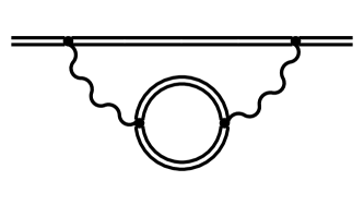
Figure 1: Two-loop self-energy diagram in Furry representation. Double lines denote electron propagators in the external electromagnetic field $A^{\mu}=\left(\,Z|e|/r,\ \boldsymbol{\mu}\times\boldsymbol{r}/r^{3}\,\right)$.

In the present paper we apply the multi-loop methods to the calculation of the contribution to the Lamb shift (LS) and to the hyperfine splitting (HFS) of the diagram, depicted in Fig. 1. The double line denotes the electron propagator in the electromagnetic field of the nucleus $A^{\mu}=\left(\,Z|e|/r,\ \boldsymbol{\mu}\times\boldsymbol{r}/r^{3}\,\right)$. Here $Z|e|$ and $\boldsymbol{\mu}$ is the nucleus charge and magnetic moment, respectively. For LS calculations we neglect the nucleus magnetic field, while for the HFS calculations we consider linear in $\boldsymbol{\mu}$ contributions. Note that the magnetic moment of the nucleus is the vector operator ${\boldsymbol{\mu}}=\mu\boldsymbol{S}/S$. However, since we consider only linear in $\boldsymbol{\mu}$ contributions, we can formally treat it as a numeric vector up to the point where we average the result over the spin wave functions.

The leading in $Z\alpha$ contribution of the diagram in Fig. 1 to LS and HFS is of the order $\mathcal{O}\left(\alpha^{2}(Z\alpha)^{4}m_{e}\right)$ and $\mathcal{O}\left(\alpha^{2}E_{F}\right)$, respectively. This contribution is completely determined by the $\propto n_{f}$ terms in the slope of the Dirac form factor and the value of the Pauli form factor of the electron at zero momentum transfer at two loops calculated long ago in Refs. Petermann:1957hs ; Barbieri:1972as . Therefore, we do not consider these contributions. Here $e$ and $m_{e}$ is the electron charge and mass, respectively,

$$E_{F}=\frac{2S+1}{3S\pi}|e|\mu(Z\alpha)^{3}m_{e}^{2}$$ (1)

is the Fermi energy, $S$ is the nucleus spin, $\alpha=e^{2}/(4\pi)\approx 1/137.036$ is the fine structure constant.

The next order contribution, $\mathcal{O}\left(\alpha^{2}(Z\alpha)^{5}m_{e}\right)$ and $\mathcal{O}\left(\alpha^{2}Z\alpha E_{F}\right)$, respectively, to LS and HFS comes from the diagrams, depicted in Figs. 2 and 3, which we will refer to as light-by-light (LbL) contribution and “free loop” (FL) contribution, respectively.

The light-by-light contributions to LS and HFS were calculated in Refs. PhysRevA.48.2609 ; Eides1994a ; Eides1993a ; Eides1994 and Eides1991 ; Kinoshita1994 , respectively. The result for the Lamb shift was presented in terms of a four-fold integral, while that for the hyperfine splitting was presented in terms of a three-fold integral. These integrals were then treated numerically. The free loop contribution to Lamb shift was obtained in terms of two-fold integrals in Refs. PhysRevA.48.2609 ; Eides1993 , while the corresponding contribution to the hyperfine splitting was obtained in Refs. Eides1990 ; Kinoshita1994 in terms of one-fold integral involving elliptic function and logarithm (or rather, arctangent).

In a sense, the result of the present paper is the representation of all four contributions (LbL and FL to LS and HFS) in the form similar to that of Ref. Eides1990 . We use modern multi-loop methods, namely, the IBP reduction Chetyrkin1981 and the differential equations method Kotikov1991 ; Remiddi1997 . In order to apply the latter, we cosider the diagrams where the mass of the fermion in the loop is different from that of the electron line. As a by-product, we also obtain the contribution of the muon loop for the ordinary hydrogen and that of electron loop for the muonic hydrogen.

2 Calculation

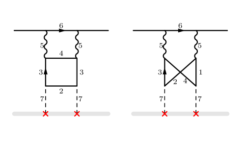
Figure 2: Gauge invariant set of diagrams which corresponds to the light-by-light contribution to the Lamb shift. Numbers correspond to the enumeration of denominators in Eq. (2).

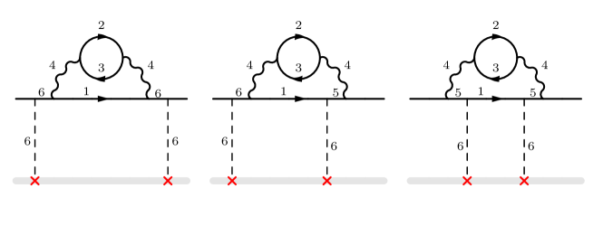
Figure 3: Gauge invariant set of diagrams which corresponds to the free-loop contribution to the Lamb shift. The second line of diagrams is a one-loop counter-terms. Numbers correspond to the enumeration of denominators in Eq. (2).

We consider the diagrams depicted in Figs. 2 and 3. The contribution of each set is gauge invariant and can be calculated independently. Note that for the HFS calculations one should replace one of the two Coulomb exchanges in those diagrams with the magnetic exchange corresponding to the contribution of the nuclear magnetic moment.

The external electron legs on the diagrams denote the bound electron wave function, however, with the precision that we pursue here, the bound-state effect is properly taken into account by the factor $|\psi_{n,l}(0)|^{2}=\delta_{l,0}\frac{(m_{e}Z\alpha)^{3}}{\pi n^{3}}$, where $\delta$ is a Kronecker symbol, $n$ and $l$ are a principal and azimuthal quantum number, correspondingly. Indeed, the characteristic loop momenta in the discussed diagrams are $k_{i}\sim m_{e}$, while that of the wave function $|\boldsymbol{p}|\sim m_{e}Z\alpha\ll m_{e}$. Therefore, we calculate the diagrams in Figs. 2 and 3 for the external electron legs corresponding to free electron with momentum $p=m_{e}\tau$, where $\tau=(1,\boldsymbol{0})$ is the time ort.

The LbL contribution is both UV and IR finite, while the FL contribution is UV and IR divergent. In order to obtain the finite result we add one-loop counter terms, depicted in Fig. 3 (second line). The two-loop counter terms, as well as the IR subtraction are expressed via scaleless integrals which are equal to zero in dimensional regularization. In particular, denoting the momentum of the Coulomb line as $k_{1}=(0,\boldsymbol{k}_{1})$, we see that the two-loop counter terms contain only one scaleless denominator $(p-k_{1})^{2}-m_{e}^{2}=k_{1}^{2}$.

The Lamb shift energy correction can be represented as

$$\delta E_{\text{LS}}=\frac{1}{2m_{e}}\overline{u}\hat{O}u|\psi_{n,l}(0)|^{2}=\frac{1}{4m_{e}}\operatorname{Tr}\left[\hat{O}(\hat{p}+m_{e})\right]|\psi_{n,l}(0)|^{2}\,,$$ (2)

where $\overline{u}\hat{O}u$ corresponds to the diagrams in Figs. 2 and 3 with both incoming and outgoing momenta equal to $p=m_{e}\tau$.

In the case of hyperfine splitting we should replace one Coulomb exchange with the magnetic exchange. Since we use the dimensional regularization, we should avoid using $\gamma^{5}$ and $\varepsilon_{ijk}$ because those objects are poorly generalized to the generic spacetime dimension $d=4-2\epsilon$. Therefore we rewrite all formulas involving vector product $(\boldsymbol{a}\times\boldsymbol{b})_{k}=\varepsilon_{ijk}a_{i}b_{j}$ in terms of antisymmetric tensors $a_{i}b_{j}-a_{j}b_{i}$. We obtain

$$\delta E_{\text{HFS}}=\frac{1}{24m_{e}}\operatorname{Tr}\left[\hat{O}^{i,j}_{\text{HFS}}(\gamma_{i}\gamma_{j}-\gamma_{j}\gamma_{i})(\hat{p}+m_{e})\right]|\psi_{n,l}(0)|^{2}\,,$$ (3)

where $\overline{u}\hat{O}^{i,j}_{\text{HFS}}u$ corresponds to the sum of the diagrams in Figs. 2 and 3 in which one of the two Coulomb exchanges $Z|e|\gamma^{0}/\boldsymbol{k}_{1}^{2}$ is replaced by the “magnetic exchange” $\mu{\gamma^{i}k_{1}^{j}}/{\boldsymbol{k}_{1}^{2}}$.

Differential system and boundary conditions.

In order to apply the differential equations method, we decouple the mass of the bound electron and the mass of the particle in the loop. We put the latter to $1$ while keeping the mass of the bound electron as a free parameter $m$.

For the light-by-light contribution we consider the integral family

$$j_{\text{LbL}}(n_{1},\ldots,n_{9})=\int\frac{dk_{1}dk_{2}dk_{3}}{\pi^{3d/2}}\prod_{k=1}^{8}\left[D_{k}+i0\right]^{-n_{k}}\times\frac{\delta^{(n_{9}-1)}\left(-D_{9}\right)}{(n_{9}-1)!}\,,$$ (4)

where

$$D_{1}=(k_{1}-k_{2}+k_{3})^{2}-1\,,\quad D_{2}=(k_{1}-k_{2})^{2}-1\,,\quad D_{3}=k_{2}^{2}-1\,,$$

$$D_{4}=(k_{2}-k_{3})^{2}-1\,,\quad D_{5}=k_{3}^{2}\,,\quad D_{6}=(k_{3}+p)^{2}-m^{2}\,,\quad D_{7}=k_{1}^{2}$$

$$D_{8}=2k_{2}\cdot p\,,\quad D_{9}=2k_{1}\cdot\tau=2k_{1}^{0}\,.$$ (5)

The $\delta$-function in Eq.(4) corresponds to zero energy transfer on the nucleus. Note that $n_{8}$ is not positive.

For the free-loop contribution we consider the family

$$j_{\text{FL}}(n_{1},\ldots,n_{9})=\int\frac{dk_{1}dk_{2}dk_{3}}{\pi^{3d/2}}\prod_{k=1}^{8}\left[\tilde{D}_{k}+i0\right]^{-n_{k}}\times\frac{\delta^{(n_{9}-1)}\left(-\tilde{D}_{9}\right)}{(n_{9}-1)!}\,,$$ (6)

where

$$\tilde{D}_{1}=(k_{1}-k_{3})^{2}-m^{2}\,,\quad\tilde{D}_{2}=k_{2}^{2}-1\,,\quad\tilde{D}_{3}=(k_{2}-k_{3})^{2}-1\,,$$

$$\tilde{D}_{4}=(k_{3})^{2}\,,\quad\tilde{D}_{5}=(p-k_{3})^{2}-m^{2}\,,\quad\tilde{D}_{6}=k_{1}^{2}\,,\quad\tilde{D}_{7}(k_{1}-k_{2})^{2}-1$$

$$\tilde{D}_{8}=2k_{2}\cdot p\,,\quad\tilde{D}_{9}=D_{9}=2k_{1}\cdot\tau=2k_{1}^{0}\,,$$ (7)

where $n_{7}$ and $n_{8}$ are not positive.

Making the IBP reduction Chetyrkin1981 ; Tkachov1981 with LiteRed Lee2014 , we reveal $14$ master integrals for light-by-light contribution and $8$ master integrals for free-loop contribution. Four master integrals are common for the two bases. Thus in the merged basis we have $14+8-4=18$ master integrals presented in Fig. 4. The first eight graphs correspond to FL basis, while the graphs $3-6$ and $9-18$ correspond to LbL basis.

Using the IBP reduction, we construct the differential equations Kotikov1991 ; Remiddi1997 for the master integrals with respect to $m^{2}$:

$$\partial_{m^{2}}\boldsymbol{j}=M\boldsymbol{j}\,,$$ (8)

where $\boldsymbol{j}=(j_{1},...,j_{18})^{\intercal}$ is a column of master integrals.

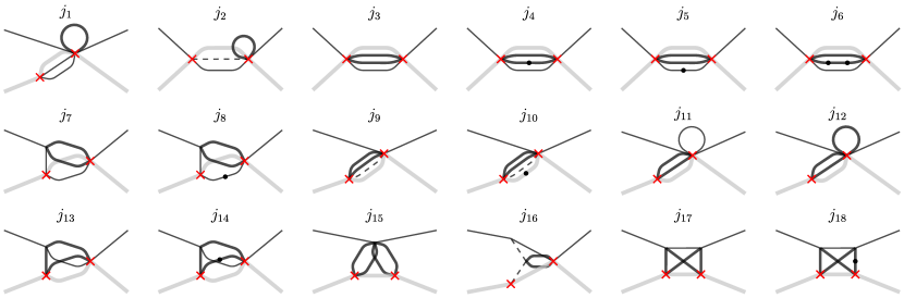
Figure 4: Basis of master integrals. Thick and thin black lines correspond to the denominators with mass $1$ and $m$, respectively. Thick gray line corresponds to $\delta(-D_{9})$, dashed lines correspond to massless denominators.

We use Libra Lee2021 to manipulate the differential system (8). We find it convenient to work with the master integrals in $2-2\epsilon$ dimensions and later express the master integrals in $4-2\epsilon$ dimensions via lowering dimensional recurrence relation Tarasov1996 . Note that the differential system (8) can not be reduced to $\epsilon$-form due to integrals $j_{3-6}$ which appear both in FL and LbL contributions. Those four master integrals can be expressed via hypergeometric functions. In particular,

$$j_{3}^{(2-2\epsilon)}=\tfrac{2^{1-8\epsilon}m^{-2\epsilon}\Gamma(4\epsilon)}{\Gamma(\epsilon+1)}\,_{4}F_{3}\left(\tfrac{1}{4}-\tfrac{\epsilon}{2},\tfrac{3}{4}-\tfrac{\epsilon}{2},\epsilon+\tfrac{1}{2},2\epsilon+\tfrac{1}{2};\tfrac{1}{2}-\epsilon,1-\epsilon,\epsilon+1;m^{2}\right)\\ -\tfrac{2^{-1-6\epsilon}\Gamma\left(2\epsilon+\tfrac{1}{2}\right)\Gamma\left(3\epsilon+\tfrac{1}{2}\right)}{\sin(\pi\epsilon)\Gamma(\epsilon+1)^{2}}\,_{4}F_{3}\left(\tfrac{\epsilon}{2}+\tfrac{1}{4},\tfrac{\epsilon}{2}+\tfrac{3}{4},2\epsilon+\tfrac{1}{2},3\epsilon+\tfrac{1}{2};\tfrac{1}{2},\epsilon+1,2\epsilon+1;m^{2}\right)\,.$$ (9)

Due to this reason the corresponding block of matrix $M$ in Eq. (8) can not be reduced in $\epsilon$-form. All other blocks can be reduced to $\epsilon$-form. With some trial and error method we have succeeded to obtain the $(A+\epsilon B)$-form of the differential equation,

$$\partial_{m^{2}}\boldsymbol{J}=M_{1}\boldsymbol{J}\,,$$ (10)

where $M_{1}(m^{2},\epsilon)=A(m^{2})+\epsilon B(m^{2})$ and the matrix $A$ has nonzero entries only in the columns $3$–$6$. We fix the boundary conditions at the point $m^{2}=0$. The general solution has the form

$$\boldsymbol{J}(m^{2})=U(M_{1}|m^{2},\underline{0})\boldsymbol{C}^{0}\,,$$ (11)

where $\boldsymbol{C}^{0}$ is a column of the boundary constants and

$$U(M|y,\underline{x})=\lim_{x_{0}\to x}\operatorname{Pexp}\left[\intop_{x_{0}}^{y}d\xi M(\xi,\epsilon)\right]x_{0}^{\operatorname*{Res}_{\xi=x}M(\xi,\epsilon)}.$$ (12)

Using Libra, we relate the boundary constants $\boldsymbol{C}^{0}$ to specific asymptotic coefficients of original master integrals $j_{1-18}$ at $m^{2}\to 0$. We compute these coefficients by using expansion-by-regions method Beneke:1997zp and direct integration of Feynman parametrization. We find that the boundary constants $\boldsymbol{C}^{0}$ are expressed in terms of the following 5 nonzero constants:

$$\left[j_{1}\right]_{m^{-1-4\epsilon}} =\left[j_{11}\right]_{m^{-2\epsilon}}=\left[j_{12}\right]_{m^{0}}=\frac{\Gamma\left(\frac{1}{2}+\epsilon\right)\Gamma\left(\frac{1}{2}+2\epsilon\right)}{2^{1+2\epsilon}\pi\epsilon}\,,\ \left[j_{2}\right]_{m^{-1-4\epsilon}}=\frac{\Gamma\left(-\frac{1}{2}-3\epsilon\right)\Gamma(4\epsilon)}{2^{-1+6\epsilon}\sqrt{\pi}\Gamma(-2\epsilon)}\,,$$

$$\left[j_{3}\right]_{m^{0}} =\left[j_{9}\right]_{m^{0}}=\frac{\Gamma\left(\frac{1}{2}+2\epsilon\right)\Gamma\left(\frac{1}{2}+3\epsilon\right)\Gamma(-\epsilon)}{2^{1+6\epsilon}\pi\Gamma(1+\epsilon)}\,,\ \left[j_{3}\right]_{m^{-2\epsilon}}=\frac{2^{1-8\epsilon}\Gamma(4\epsilon)}{\Gamma(1+\epsilon)}\,,$$

$$\left[j_{15}\right]_{m^{0}}=j^{(2-2\epsilon)}_{15}=\frac{2^{1+2\epsilon}\Gamma(-4\epsilon)\Gamma\left(\frac{1}{2}+2\epsilon\right)\Gamma\left(\frac{3}{2}+3\epsilon\right)}{4(1+2\epsilon)\Gamma\left(\frac{1}{2}-\epsilon\right)^{2}\tan(\pi\epsilon)}\\ +\frac{\Gamma\left(\frac{1}{2}+2\epsilon\right)\Gamma\left(\frac{1}{2}+\epsilon\right)}{4^{1+\epsilon}\pi}\bigg{[}\,_{3}F_{2}\left(1,-\epsilon,\epsilon+1;\tfrac{3}{2},\tfrac{1}{2}-2\epsilon;1\right)\\ -\frac{4\epsilon+1}{4\epsilon(\epsilon+1)}\,_{3}F_{2}\left(\tfrac{1}{2},1,2\epsilon+\tfrac{3}{2};1-\epsilon,\epsilon+2;1\right)\bigg{]}\,,$$ (13)

where $[j_{k}]_{m^{\nu}}$ denotes the coefficient in front of ${m^{\nu}}$ in the small-mass asymptotics of $j_{k}^{(2-2\epsilon)}$.

All but the last constant are trivially expressed in terms of alternating multiple zeta values. It is not obvious which transcendental numbers might enter the expansion of the last constant $j_{15}^{(2-2\epsilon)}$. Nevertheless, using the PSLQ and our experience, we have been able to establish that the $\epsilon$-expansion of $j_{15}^{(2-2\epsilon)}$ can be written in terms of Goncharov’s polylogarithms at fourth root of unity. The two first terms of $\epsilon$-expansion read

$$j_{15}^{(2-2\epsilon)}=e^{-3\epsilon\gamma_{E}}\left[\tfrac{1}{2}-\tfrac{\pi}{8}+\left(2G+\tfrac{3}{2}\pi\ln 2-4\ln 2-\tfrac{\pi}{2}-1\right)\epsilon+\mathcal{O}\left(\epsilon^{2}\right)\right]\,,$$ (14)

where $G=\operatorname{Im}{\text{Li}_{2}(i)}=\sum_{k=0}^{\infty}\frac{(-1)^{k}}{(2k+1)^{2}}=0.915965594...$ is the Catalan constant. For our present goal we will need only the leading term of this expansion.

$\epsilon$-regular basis

Since the differential system (8) for the master integrals can not be reduced to $\epsilon$-form, we should rely on the Frobenius method for the calculation of the evolution operator $U(m^{2},\underline{0})$ in Eq. (12). The dependence of this operator on $\epsilon$ constitutes substantial technical difficulties and blocks the way to high-precision numerical calculation suitable for the application of PSLQ algorithm, ferguson1999analysis , for the recognition of the master integrals in the point $m=1$. Thus we choose to switch to the $\epsilon$-regular basis Lee2019_eps . After finding this basis, we simply put $\epsilon=0$.

Note that the counter-term diagrams in the second line of Fig. 3 can also be expressed in terms of the three-loop master integrals in Fig. 4 although they have only two loops. To this end we multiply the corresponding integrals by $1=\frac{-1}{\Gamma[1-d/2]}\int\frac{d^{d}k_{2}}{i\pi^{d/2}D_{2}}$. Then the contribution of counter-terms is expressed via the master integrals with unit mass tadpole loop, namely, via $j_{1},\ j_{2}$. Luckily, $\Gamma[1-d/2]$ in the denominators cancels with the same $\Gamma$ in $\delta Z_{3}^{(1l)}=-\frac{4\Gamma(2-d/2)\alpha}{3(4\pi)^{d/2-1}}=-\frac{4(1-d/2)\Gamma(1-d/2)\alpha}{3(4\pi)^{d/2-1}}$ which stands for the cross in the couter-term diagrams. Therefore, the finite sum of all diagrams in Fig. 3 is expressed via the integrals of the family (6) with rational coefficients. Then we are in position to state the existence of $\epsilon$-regular basis Lee2019_eps .

Let us describe how we construct this $\epsilon$-regular basis.

1. We start from the found $(A+\epsilon B)$-form. Thus, the coefficients of differential equations are regular in the limit $\epsilon\to 0$.

2. We determine the highest leading term $\mathcal{O}(\epsilon^{-n})$ in $\epsilon$-expansion of the boundary constants. We multiply all integrals by $\epsilon^{n}$ to make all new functions $\boldsymbol{J}$ finite. The two next steps are performed in the loop over the row number $i$.

3. Then we use the following rule of thumb: if for, say, $J_{i}$ function both the boundary constant $C_{i}$ and the right-hand side of the equation are zero at $\epsilon=0$ is zero, then the function itself is also zero at $\epsilon=0$. Therefore, we redefine $J_{i}\to\epsilon J_{i}$ and modify respectively the boundary constant $C_{i}\to\epsilon C_{i}$ and the differential system. The latter modification is reduced to the multiplication/division by $\epsilon$ the $i$-th column/row of the matrix $A+\epsilon B$.

4. We also use substitutions of the form $J_{i}\to J_{i}+\sum_{k<i}c_{k}J_{k}$, where the coefficients $c_{k}$ are rational numbers chosen so as to nullify as many entries on the $i$-th row of the matrix $M(m^{2},0)$ as possible.

This approach works perfectly for all rows except for the rows $3-6$ corresponding to the equations irreducible to $\epsilon$-form. For those $4$ master integrals we use the presumable finiteness of the sum of diagrams in Figs. 2,3 as a guiding line for finding the relations between $j_{3-6}$ near $d=2$. We find that

$$Q(m^{2},\epsilon)=\left(1-m^{2}\right)\left(2+m^{2}\epsilon+12\epsilon\right)j_{3}+\left(78m^{4}\epsilon-25m^{4}-72m^{2}\epsilon+36m^{2}-8\right)j_{4}\\ -m^{2}\left(4-m^{2}+6m^{2}\epsilon\right)j_{5}-48\left(1-m^{2}\right)m^{2}(1-4\epsilon)j_{6}=\mathcal{O}(\epsilon^{2})$$ (15)

Thus we choose $J(m^{2},\epsilon)=Q(m^{2},\epsilon)/\epsilon^{2}$ as an element of $\epsilon$-regular basis. Indeed, we see that after this choice both the boundary constants and the matrix $M(m^{2},\epsilon)$ have finite limit $\epsilon\to 0$.

The result of our approach is the differential system in which we can simply put $\epsilon=0$. The higher orders in $\epsilon$ which we miss with putting $\epsilon$ to zero are guaranteed not to appear in our final results, which is the rationale behind the notion of $\epsilon$-regular basis. The resulting system has the form

$$\partial_{m^{2}}\boldsymbol{J}_{\text{reg}}=\overline{M}(m^{2})\boldsymbol{J}_{\text{reg}}\,,$$ (16)

where the matrix $\overline{M}$ is strictly lower triangular except for the diagonal $4\times 4$ block with indices $3$–$6$. It is essential that $\overline{M}$ does not depend on $\epsilon$. The singular points of the differential system are $m^{2}=0,1,\infty$. Again, we write the solution in the form

$$\boldsymbol{J}_{\text{reg}}(m^{2})=U(\overline{M}|m^{2},\underline{0})\boldsymbol{C}^{0}\,.$$ (17)

The almost lower triangular structure of the matrix $M$ allows us to write the general solution in terms of polylogarithms and/or one-fold integrals of $j_{3-6}$ multiplied by polylogarithms. However we choose here to construct the Frobenius expansions near each of the three singular points of the differential system (17), $m^{2}=0,1,\infty$. We match the obtained expansions pairwise in the points which belong to the intersection of convergence regions of the corresponding two expansions. For example the expansions near $m^{2}=0$ and $m^{2}=1$ are connected via the relation

$$\boldsymbol{J}_{\text{reg}}(1/2)=U(\overline{M}|1/2,\underline{0})\boldsymbol{C}^{0}=U(\overline{M}|1/2,\underline{1})\boldsymbol{C}^{1}\,.$$ (18)

Then the boundary constants at $m^{2}=1$ are expressed as $\boldsymbol{C}^{1}=U^{-1}(\overline{M}|\tfrac{1}{2},\underline{1})U(\overline{M}|\tfrac{1}{2},\underline{0})\boldsymbol{C}^{0}$. We calculate $1000$ terms of series of $U(1/2,\underline{1})$ and $U(1/2,\underline{0})$ and compute more than $300$ digits for $\boldsymbol{C}^{1}$. In order to use PSLQ recognition, we need to have a basis of appropriate transcendental numbers and we extract all but one required nontrivial constants from Ref. Eides1990 . Therein the result for the FL contribution to HFS was expressed in terms of the weighted sum of the integrals (cf. Eq. (11) of Ref. Eides1990 )

$$\{c_{1},c_{2},c_{3},c_{4}\}=\intop_{0}^{1}\frac{dq}{q^{2}}[\mathrm{K}(q^{2})-\mathrm{E}(q^{2})]\left\{\frac{\arctan\left(\sqrt{\frac{2q}{1-q}}\right)}{1+q},\,\frac{\sqrt{\frac{2q}{1-q}}}{1+q},\,\sqrt{\frac{2q}{1-q}},\,q\sqrt{\frac{2q}{1-q}}\right\}\,,$$ (19)

where $\mathrm{K}(x)$ and $\mathrm{E}(x)$ are complete elliptic integrals. Moreover, using PSLQ it is easy to establish a relation $6c_{2}-5c_{3}+2c_{4}=0$ overlooked in Ref. Eides1990 . Using some guess work, we find the following basis sufficient for our purpose

$$\boldsymbol{B} =\{1,\pi,\ln 2,\pi^{2},\zeta_{3},e_{0},1/e_{0},e_{1},e_{2}\}\,,$$

$$e_{0} =\frac{3}{4\pi}\intop_{0}^{1}\frac{dq\,\mathrm{K}(q^{2})}{1+q}\sqrt{\frac{2q}{1-q}}=\tfrac{\Gamma(3/8)\Gamma(9/8)}{\Gamma(5/8)\Gamma(7/8)}=1.42812528609616838918477155113\ldots\,,$$

$$e_{1} =\frac{2}{\pi}\intop_{0}^{1}\frac{dq\,\mathrm{K}(q^{2})}{1+q}\arctan\left(\sqrt{\frac{2q}{1-q}}\right)=0.70733097502159315134278673801\ldots\,,$$

$$e_{2} =\frac{2}{\pi}\intop_{0}^{1}\frac{dq\,\mathrm{K}(q^{2})}{1+q}\operatorname{Im}\mathrm{Li}_{2}\left(i\sqrt{\frac{2q}{1-q}}\right)=1.08354966910460443406693681278\ldots\,,$$ (20)

where $\mathrm{Li}_{2}(x)$ is a dilogarithm. The constants $c_{1-4}$ in Eq. (19) are expressed as linear combinations with rational coefficients of $\{1,e_{0},1/e_{0},e_{1}\}$:

$$c_{1}=\tfrac{1}{2e_{0}}-\tfrac{7e_{0}}{6}+e_{1}+1,\quad c_{2}=\tfrac{1}{e_{0}}+\tfrac{e_{0}}{3},\quad c_{3}=\tfrac{1}{e_{0}}+e_{0},\quad c_{4}=\tfrac{3e_{0}}{2}-\tfrac{1}{2e_{0}}\,.$$ (21)

The benefit of using $e_{0},e_{0}^{-1},$ and especially $e_{1}$ instead of $c_{1-4}$ is that their form allowed us to guess the form of the last nonstandard constant $e_{2}$, which was deduced from $e_{1}$ by noting that $\arctan\left(x\right)=\operatorname{Im}\mathrm{Li}_{1}(ix)$ and then replacing $\mathrm{Li}_{1}\to\mathrm{Li}_{2}$. To obtain the contributions to the Lamb shift and the hyperfine splitting we need a few coefficients of the expansion of $J_{\text{reg}}(m^{2})$ near the point $m^{2}=1$. This expansion has the form

$$\boldsymbol{J}_{\text{reg}}(m^{2})=U(\overline{M}|m^{2},\underline{1})\boldsymbol{C}^{1}\,,$$ (22)

where $U(\overline{M}|m^{2},\underline{1})$ has the form of generalized power series in $1-m^{2}$. In particular, $U(m^{2},\underline{1})$ contains $\ln(1-m^{2})$. However, we have checked that these logarithms disappear when $U(m^{2},\underline{1})$ is multiplied by $\boldsymbol{C}^{1}$ so that the specific solution has no branching at the point $m^{2}=1$ as it should be.

The power series (22) converge when $m^{2}\in(0,2)$. To obtain the results for $\boldsymbol{J}_{\text{reg}}(m^{2})$ at $m^{2}>2$ we pass to the variable $z=\frac{m^{2}-1}{m^{2}}$ and again match the power series near $z=0$ ($m^{2}=1$) and $z=1$ ($m^{2}=\infty$) at $z=1/2$. In this way we obtain the high-precision numerical result for the column of boundary constants $\boldsymbol{C}^{\infty}$ which define the coefficients in the asymptotic expansion of $\boldsymbol{J}_{\text{reg}}(m^{2})$ at $m^{2}\to\infty$. In order to define the analytic form of $\boldsymbol{C}^{\infty}$ we again use PSLQ recognition with the following basis:

$$\boldsymbol{B}_{\infty}=(1,\pi,\ln 2,\pi^{2},\ln^{2}2,\zeta_{3},i_{0},1/i_{0})\,,\qquad i_{0}=\tfrac{\Gamma(5/4)^{2}}{\Gamma(3/4)^{2}}\,.$$ (23)

The nontrivial constants $i_{0}$ and $i_{0}^{-1}$ were conjectured by examining the large-mass asymptotics of $j_{3}$ from Eq. (9).

3 Results

The discussed corrections to the Lamb shift and hyperfine splitting have the following form

$$\delta E^{i}_{\text{LS}} =\delta_{l,0}\frac{\alpha^{2}(Z\alpha)^{5}}{\pi n^{3}}m_{e}\left(\frac{m_{r}}{m_{e}}\right)^{3}B_{i}\,,$$

$$\delta E^{i}_{\text{HFS}} =\delta_{l,0}\frac{\alpha^{2}(Z\alpha)}{\pi n^{3}}E_{F}\left(\frac{m_{r}}{m_{e}}\right)^{3}C_{i}\,,$$ (24)

where $i=FL,LbL$ for different contributions and we have recovered the recoil factor $\left(\frac{m_{r}}{m_{e}}\right)^{3}=\left(\frac{M}{M+m_{e}}\right)^{3}$ accounting the main effect of the finite nuclear mass $M$.

For the case of electron loop in electron atom we have the following result:

$$B_{FL} =-\frac{17267}{7560}-\frac{241}{324e_{0}}+\frac{296767e_{0}}{132300}-\frac{2e_{1}}{3}=-0.072909964469261993898\ldots\,,$$

$$B_{LbL} =\frac{21401}{540}-\frac{383}{54e_{0}}-\frac{11e_{0}}{10}+\frac{10e_{1}}{3}+\frac{16e_{2}}{9}+\frac{13\pi}{36}-\frac{\pi^{2}}{12}-\frac{406}{9}\ln{2}-\frac{49}{9}\zeta_{3}$$

$$\mspace{303.0mu}=-0.12291622969679641051\ldots\,,$$

$$C_{FL} =-\frac{59}{270}-\frac{343}{1296e_{0}}-\frac{1079e_{0}}{10800}+\frac{e_{1}}{3}=-0.31074204276601754458\ldots\,,$$

$$C_{LbL} =46-\frac{39}{2e_{0}}-\frac{23e_{0}}{6}+16e_{1}+\frac{40e_{2}}{9}-\frac{\pi^{2}}{2}-32\ln{2}-\frac{245}{18}\zeta_{3}$$

$$\mspace{267.0mu}=-0.47251462820471059187\ldots\,.$$ (25)

Given the representation of Eq. (2) for the constants $e_{0}$, $e_{1}$, $e_{2}$, the above expressions provide a one-fold integral representation for the corresponding contributions to Lamb shift and hyperfine splitting. The numerical values for $B_{FL}$, $B_{LbL}$, $C_{FL}$, $C_{LbL}$ agree with the results of Refs. PhysRevA.48.2609 ; Eides1993 ; Eides1994a ; Eides1994 ; Eides1990 ; Eides1993a ; Kinoshita1994 . For the case of muon loop in electron atom we have the following result:

$$B_{FL} =-\frac{7}{60}\left(\tfrac{m_{e}}{m_{\mu}}\right)+\frac{109}{1512}\left(\tfrac{m_{e}}{m_{\mu}}\right)^{2}-\frac{3}{56}\left(\tfrac{m_{e}}{m_{\mu}}\right)^{3}+\mathcal{O}\left(\left(\tfrac{m_{e}}{m_{\mu}}\right)^{4}\right)\,,$$

$$B_{LbL} =\left[\frac{470561}{21600}-\frac{437\pi}{720}-\frac{27647}{960}\ln{2}+\frac{281}{2304}\ln\left(\tfrac{m_{e}}{m_{\mu}}\right)\right]\left(\tfrac{m_{e}}{m_{\mu}}\right)^{2}+\mathcal{O}\left(\left(\tfrac{m_{e}}{m_{\mu}}\right)^{4}\right)\,,$$

$$C_{FL} =-\frac{1}{3}\left(\tfrac{m_{e}}{m_{\mu}}\right)+\frac{1751}{30240}\left(\tfrac{m_{e}}{m_{\mu}}\right)^{3}+\mathcal{O}\left(\left(\tfrac{m_{e}}{m_{\mu}}\right)^{4}\right)\,,$$

$$C_{LbL} =\left[\frac{5}{24}-2\pi+8\ln{2}\right]\left(\tfrac{m_{e}}{m_{\mu}}\right)$$

$$+\left[\frac{6931861}{552960}-\frac{\pi}{3}-\frac{38107}{2304}\ln{2}-\frac{805}{9216}\ln\left(\tfrac{m_{e}}{m_{\mu}}\right)\right]\left(\tfrac{m_{e}}{m_{\mu}}\right)^{3}+\mathcal{O}\left(\left(\tfrac{m_{e}}{m_{\mu}}\right)^{4}\right)\,.$$ (26)

One is tempted to obtain also the results for the contribution of the electron loop in the muonic hydrogen by making a substitution $m_{e}\to m_{\mu}$ in Eq. (3) and using the large-$m$ asymptotics of $\boldsymbol{J}_{\text{reg}}$. Then the results for functions $B_{i}$ and $C_{i}$ have the following form

$$B_{FL} =-i_{0}\frac{1600}{441}\sqrt{\tfrac{m_{e}}{m_{\mu}}}+\mathcal{O}\left(\tfrac{m_{e}}{m_{\mu}}\right)\,,$$ (27)

$$B_{LbL} =\left(-\frac{139}{18}+\frac{2\pi^{2}}{3}+\frac{4}{3}\ln{2}\right)\tfrac{m_{\mu}}{m_{e}}+\frac{4187}{135}+\frac{7\pi}{36}-\frac{406}{9}\ln{2}+\mathcal{O}\left(\tfrac{m_{e}}{m_{\mu}}\right)\,,$$

$$C_{FL} =\left(-\frac{13}{6}+\frac{2}{3}\ln{2}\right)\ln\left(\tfrac{m_{\mu}}{m_{e}}\right)+\frac{379}{72}-\frac{14}{9}\ln{2}-\frac{\pi^{2}}{18}+\frac{1}{3}\ln^{2}{2}-\frac{72}{25i_{0}}\sqrt{\tfrac{m_{e}}{m_{\mu}}}+\mathcal{O}\left(\tfrac{m_{e}}{m_{\mu}}\right)\,,$$

$$C_{LbL} =\left(12+4\ln{2}-\frac{5\pi^{2}}{3}\right)\ln\left(\tfrac{m_{\mu}}{m_{e}}\right)-13+\frac{5\pi^{2}}{6}+2\ln^{2}{2}+5\zeta_{3}+\mathcal{O}\left(\tfrac{m_{e}}{m_{\mu}}\right)\,.$$

However, for muonic atom the characteristic momenta of bound muon (or the inverse size of its wave funcetion), $m_{\mu}Z\alpha$ is of the same order, or larger, as the characteristic loop momenta $m_{e}$ even for $Z=1$. Therefore, the applicability condition for the approximation used in the present paper is violated and Eq. (27) may be considered at most as an order of magnitude estimate.

4 Conclusion

In the present paper we revisit the contributions of order $\alpha^{2}(Z\alpha)^{5}m$ to the Lamb shift and of the order $\alpha^{2}(Z\alpha)E_{F}$ to the hyperfine splitting from mixed self-energy-vacuum-polarization diagrams depicted in Figs. 2 and 3. We construct the $\epsilon$-regular basis Lee2019_eps and explicitly demonstrate that its elements taken at $\epsilon=0$ are sufficient to express the renormalized results. The results have the form of one-fold integral involving elliptic function and dilogarithm and agree with previously known numerical results. We also obtain the contribution of the same set of diagrams with different mass of the fermion in the loop and in the fermion line, which allows us to determined the corresponding contribution of the muonic loop in the conventional hydrogen as well as the estimate of the electron loop contribution in the muonic hydrogen.

- (1) R. Karplus, A. Klein and J. Schwinger, Electrodynamic displacement of atomic energy levels, Physical Review 84 (1951) 597.
- (2) H. A. Bethe, The electromagnetic shift of energy levels, Physical Review 72 (1947) 339.
- (3) N. M. Kroll and F. Pollock, Radiative corrections to the hyperfine structure and the fine structure constant, Physical Review 84 (1951) 594.
- (4) R. Karplus and A. Klein, Electrodynamic displacement of atomic energy levels. i. hyperfine structure, Physical Review 85 (1952) 972.
- (5) M. I. Eides, H. Grotch and V. A. Shelyuto, Theory of Light Hydrogenic Bound States, vol. 222. Springer-Verlag, Berlin, 2007, 10.1007/3-540-45270-2.
- (6) A. Petermann, Fourth order magnetic moment of the electron, Helv. Phys. Acta 30 (1957) 407.
- (7) R. Barbieri, J. A. Mignaco and E. Remiddi, Electron form-factors up to fourth order. 1., Nuovo Cim. A 11 (1972) 824.
- (8) K. Pachucki, Contributions to the binding, two-loop correction to the lamb shift, Phys. Rev. A 48 (1993) 2609.
- (9) M. I. Eides, H. Grotch and P. Pebler, (zm contribution to the hydrogen lamb shift from virtual light-by-light scattering, Phys. Rev. A 50 (1994) 144.
- (10) M. Eides, S. Karsenboim and V. Shelyuto, Purely radiative contribution to muonium and hydrogen hyperfine splitting induced by light by light scattering insertion in external photons: (phys. lett. b 268 (1991) 433; b 316 (1993) 631 (e)), Physics Letters B 319 (1993) 545.
- (11) M. I. Eides, H. Grotch and P. Pebler, Light by light scattering contribution to lamb shift in hydrogen, Physics Letters B 326 (1994) 197.
- (12) M. I. Eides, S. G. Karshenboim and V. A. Shelyuto, Purely radiative contribution to muonium and hydrogen hyperfine splitting induced by light by light scattering insertion in external photons, Physics Letters B 268 (1991) 433.
- (13) T. Kinoshita and M. Nio, Improved theory of the muonium hyperfine structure, Phys. Rev. Lett. 72 (1994) 3803.
- (14) M. I. Eides and H. Grotch, New correction to lamb shift induced by one-loop polarization insertions in the radiative electron factor, Physics Letters B 308 (1993) 389.
- (15) M. I. Eides, S. G. Karshenboim and V. A. Shelyuto, Last vacuum polarization contribution of order to muonium and hydrogen hyperfine splitting, Physics Letters B 249 (1990) 519.
- (16) K. Chetyrkin and F. Tkachov, Integration by parts: The algorithm to calculate -functions in 4 loops, Nuclear Physics B 192 (1981) 159.
- (17) A. Kotikov, Differential equations method. new technique for massive feynman diagram calculation, Physics Letters B 254 (1991) 158.
- (18) E. Remiddi, Differential equations for feynman graph amplitudes, Il Nuovo Cimento A (1971-1996) 110 (1997) 1435.
- (19) F. Tkachov, A theorem on analytical calculability of 4-loop renormalization group functions, Physics Letters B 100 (1981) 65.
- (20) R. N. Lee, Litered 1.4: a powerful tool for reduction of multiloop integrals, Journal of Physics: Conference Series 523 (2014) 012059.
- (21) R. N. Lee, Libra: A package for transformation of differential systems for multiloop integrals, Computer Physics Communications 267 (2021) 108058.
- (22) O. V. Tarasov, Connection between feynman integrals having different values of the space-time dimension, Phys. Rev. D 54 (1996) 6479 [hep-th/9606018].
- (23) M. Beneke and V. A. Smirnov, Asymptotic expansion of Feynman integrals near threshold, Nucl. Phys. B 522 (1998) 321 [hep-ph/9711391].
- (24) H. Ferguson, D. Bailey and S. Arno, Analysis of pslq, an integer relation finding algorithm, Mathematics of Computation 68 (1999) 351.
- (25) R. Lee and A. Onishchenko, -regular basis for non-polylogarithmic multiloop integrals and total cross section of the process , Journal of High Energy Physics (2019) .