An Approximate Projection onto the Tangent Cone to the Variety of Third-Order Tensors of Bounded Tensor-Train Rank
Abstract
An approximate projection onto the tangent cone to the variety of third-order tensors of bounded tensor-train rank is proposed and proven to satisfy a better angle condition than the one proposed by Kutschan (2019). Such an approximate projection enables, e.g., to compute gradient-related directions in the tangent cone, as required by algorithms aiming at minimizing a continuously differentiable function on the variety, a problem appearing notably in tensor completion. A numerical experiment is presented which indicates that, in practice, the angle condition satisfied by the proposed approximate projection is better than both the one satisfied by the approximate projection introduced by Kutschan and the proven theoretical bound.
Keywords:
Projection Tangent cone Angle condition Tensor-train decomposition.1 Introduction
Tangent cones play an important role in constrained optimization to describe admissible search directions and to formulate optimality conditions [9, Chap. 6]. In this paper, we focus on the set
| (1) |
where denotes the tensor-train rank of (see Section 2.2), which is a real algebraic variety [4], and, given , we propose an approximate projection onto the tangent cone , i.e., a set-valued mapping such that there exists such that, for all and all ,
| (2) |
where is the inner product on given in [1, Example 4.149], is the induced norm, and the set
| (3) |
is the projection of onto . By [10, Definition 2.5], inequality (2) is called an angle condition; it is well defined since, as is a closed cone, all elements of have the same norm (see Section 3). Such an approximate projection enables, e.g., to compute a gradient-related direction in , as required in the second step of [10, Algorithm 1] if the latter is used to minimize a continuously differentiable function on , a problem appearing notably in tensor completion; see [11] and the references therein.
An approximate projection onto satisfying the angle condition (2) with was proposed in [5, §5.4]. If is a singular point of the variety, i.e., , the approximate projection proposed in this paper ensures (see Theorem 3.1)
| (4) |
which is better, and can be computed via SVDs (see Algorithm 1). We point out that no general formula to project onto the closed cone , which is neither linear nor convex (see Section 2.3), is known in the literature.
This paper is organized as follows. Preliminaries are introduced in Section 2. Then, in Section 3, we introduce the proposed approximate projection and prove that it satisfies (2) with as in (4) (Theorem 3.1). Finally, in Section 4, we present a numerical experiment where the proposed approximate projection preserves the direction better than the one from [5, §5.4].
2 Preliminaries
In this section, we introduce the preliminaries needed for Section 3. In Section 2.1, we recall basic facts about orthogonal projections. Then, in Section 2.2, we review the tensor-train decomposition. Finally, in Section 2.3, we review the description of the tangent to given in [4, Theorem 2.6].
2.1 Orthogonal Projections
Given with , we let denote the Stiefel manifold. For every , we let and denote the orthogonal projections onto the range of and its orthogonal complement, respectively. The proof of Theorem 3.1 relies on the following basic result.
Lemma 1
Let have rank . If is a truncated SVD of rank of , with , then, for all and all ,
| (5) | ||||
| (6) |
Proof
By the Eckart–Young theorem, is a projection of onto
Thus, since is a closed cone, the same conditions as in (14) hold. Moreover, since and thus , it holds that
Furthermore, for all , Hence,
Thus, The left inequality in (5) follows, and the one in (6) can be obtained similarly.
By orthogonal invariance of the Frobenius norm and by definition of ,
where are the singular values of in decreasing order. Moreover, either or . In the first case, we have
In the second case, we have
Thus, in both cases, the second inequality in (5) holds. The second inequality in (6) can be obtained in a similar way. ∎
2.2 The Tensor-Train Decomposition
In this section, we review basic facts about the tensor-train decomposition (TTD) that are used in Section 3; we refer to the original paper [8] and the subsequent works [3, 11, 12] for more details.
A tensor-train decomposition of is a factorization
| (7) |
where , , , and ‘’ denotes the contraction between a matrix and a tensor. The minimal for which a TTD of exists is called the TT-rank of and is denoted by . By [2, Lemma 4], the set
| (8) |
is a smooth embedded submanifold of .
Let and denote respectively the left and right unfoldings of . Then, and the minimal rank decomposition can be obtained by computing two successive SVDs of unfoldings; see [8, Algorithm 1]. The contraction interacts with the unfoldings according to the following rules:
For every , if , then the mode- vectors of are the orthogonal projections onto the range of of those of . A similar property holds for . The tensor is said to be left-orthogonal if and , and right-orthogonal if and .
As a TTD is not unique, certain orthogonality conditions can be enforced, which can improve the numerical stability of algorithms working with TTDs. Those used in this work are given in Lemma 2.
2.3 The Tangent Cone to the Low-Rank Variety
In [4, Theorem 2.6], a parametrization of the tangent cone to is given and, because this parametrization is not unique, corresponding orthogonality conditions are added. The following lemma recalls this parametrization however with slightly different orthogonality conditions which make the proofs in the rest of the paper easier, and the numerical computations more stable because they enable to avoid matrix inversion in Algorithm 1.
Lemma 2
Let have as TTDs, where , , , and . Then, is the set of all such that
| (9) |
with , , , , , , , , for all , and
| (10) | ||||||||
Proof
By [4, Theorem 2.6], is the set of all that can be decomposed as
with the orthogonality conditions
| (11) | ||||||||
The following invariances hold for all , and :
Then, if we define , , , , , , , and , the matrices , , , and can be chosen such that is left-orthogonal, , , and , e.g., using SVDs. Additionally, can be decomposed as . The two terms involving and can then be regrouped as
where we have defined , obtaining the parametrization (9) satisfying (10). ∎
3 The Proposed Approximate Projection
In this section, we prove Proposition 1 and then use it to prove Theorem 3.1. Both results rely on the following observation. By [6, Proposition A.6], since is a closed cone, for all and , it holds that or, equivalently, . Thus, all elements of have the same norm and (3) can be rewritten as
| (14) |
Proposition 1
Proof
Straightforward computations show that and . Thus, is a feasible point of (14). Since is a solution to (14), . Therefore, if , then and consequently all parameters in (1) are zero because of (2.3). Otherwise, by using the Cauchy–Schwarz inequality, we have
| (16) |
where the last inequality holds because is a solution to (14). It follows that the Cauchy–Schwarz inequality is an equality and hence there exists such that . By (16), . Thus, because of (2.3), the parameters in (1) are those of . ∎
Theorem 3.1
Let be as in Lemma 2 with . The approximate projection that computes the parameters and of in (12) with Algorithm 1 and the parameters , , , , , and with (1) satisfies (2) with as in (4) for all and all in Algorithm 1.
Proof
Let and . Thus, . Because , , , , , and are as in (1), it holds that , thus is a feasible point of (14), and hence (2) is equivalent to . To compare the norm of with the norm of , and are defined as the parameters of . From (1), and because all terms are mutually orthogonal, we have that
Now, assume that and consider the first iteration of Algorithm 1. Because in the second step is obtained by a truncated SVD of and, by using (6),
Furthermore, because in the first step is obtained from the truncated SVD of and by using (5),
where we have used that a multiplication with can only decrease the norm. The same is true for a multiplication with and thus
In Algorithm 1, the norm of the approximate projection increases monotonously. Thus, this lower bound is satisfied for any and . A similar derivation can be made if . ∎
This section ends with three remarks on Algorithm 1. First, the instruction “” means that is a truncated SVD of rank of . Since those SVDs are not necessarily unique, Algorithm 1 can output several for a given input, and hence the approximate projection is set-valued.
Second, the most computationally expensive operation in Algorithm 1 is the truncated SVD. The first step of the first iteration requires to compute either singular vectors of a matrix of size or singular vectors of a matrix of size . All subsequent steps are computationally less expensive since each of them merely requires to compute either singular vectors of or singular vectors of , and, in general, and . This is because
and the rightmost matrix, being in by Lemma 2, does not change the left singular vectors (and values). The argument for is similar. The Matlab implementation of Algorithm 1 that is used to perform the numerical experiment in Section 4 computes a subset of singular vectors (and singular values) using the svd function with ‘econ’ flag.
Third, studying the numerical stability of Algorithm 1 would require a detailed error analysis, which is out of the scope of the paper. Nevertheless, the modified orthogonality conditions improve the stability compared to the approximate projection described in [5, §5.4.4] because Algorithm 1 uses only orthogonal matrices to project onto vector spaces (it uses no Moore–Penrose inverse).
4 A Numerical Experiment
To compute gradient-related directions in the tangent cone, the input tensor for Algorithm 1 would be the gradient of the continuously differentiable function that is considered. Since, in general, such tensors are dense, we consider in this section randomly generated pairs of dense tensors with and , and compare the values of obtained by computing the approximate projection of onto using Theorem 3.1, the tensor diagrams from [5, §5.4.4], which we have implemented in Matlab, and the point output by the built-in Matlab function fmincon applied to (3). The latter can be considered as a benchmark for the exact projection. Since , (2) is satisfied if .
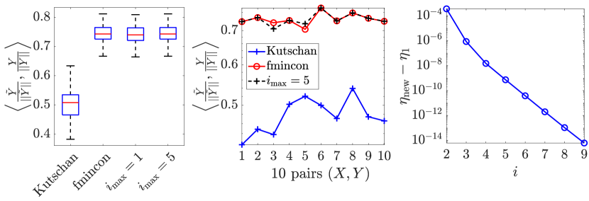
For this experiment, we set and generate fifty random pairs , where and , using the built-in Matlab function randn. For such pairs, the from (4) equals . We use Algorithm 1 with , which implies that is used as stopping criterion. In the left subfigure of Figure 1, the box plots for this experiment are shown for two values of . As can be seen, for both values of , the values of obtained by the proposed approximate projection are close to those obtained by fmincon and are larger than those obtained by the approximate projection from [5, §5.4]. We observe that is always larger than , which suggests that (4) is a pessimistic estimate. The middle subfigure compares ten of the fifty pairs. For one of these pairs, the proposed method obtains a better result than fmincon. This is possible since the fmincon solver does not necessarily output a global solution because of the nonconvexity of (3). An advantage of the proposed approximate projection is that it requires less computation time than the fmincon solver (a fraction of a second for the former and up to ten seconds for the latter). In the rightmost subfigure, the evolution of is shown for one of the fifty pairs. This experiment was run on a laptop with a AMD Ryzen 7 PRO 3700U processor (4 cores, 8 threads) having 13.7 GiB of RAM under Kubuntu 20.04. The Matlab version is R2020a. The code is publicly available.111URL: https://github.com/golikier/ApproxProjTangentConeTTVariety
References
- [1] Hackbusch, W.: Tensor Spaces and Numerical Tensor Calculus, Springer Series in Computational Mathematics, vol. 56. Springer Cham, 2nd edn. (2019)
- [2] Holtz, S., Rohwedder, T., Schneider, R.: On manifolds of tensors of fixed TT-rank. Numer. Math. 120(4), 701–731 (2012)
- [3] Kressner, D., Steinlechner, M., Uschmajew, A.: Low-Rank Tensor Methods with Subspace Correction for Symmetric Eigenvalue Problems. SIAM J. Sci. Comput. 36(5), A2346–A2368 (2014)
- [4] Kutschan, B.: Tangent cones to tensor train varieties. Linear Algebra Appl. 544, 370–390 (2018)
- [5] Kutschan, B.: Convergence of Gradient Methods on Hierarchical Tensor Varieties. Ph.D. thesis, TU Berlin (2019)
- [6] Levin, E., Kileel, J., Boumal, N.: Finding stationary points on bounded-rank matrices: A geometric hurdle and a smooth remedy. Math. Program. (2022)
- [7] Lubich, C., Oseledets, I.V., Vandereycken, B.: Time Integration of Tensor Trains. SIAM J. Numer. Anal. 53(2), 917–941 (2015)
- [8] Oseledets, I.V.: Tensor-Train Decomposition. SIAM J. Sci. Comput. 33(5), 2295–2317 (2011)
- [9] Rockafellar, R.T., Wets, R.J.B.: Variational Analysis, Grundlehren der mathematischen Wissenschaften, vol. 317. Springer-Verlag Berlin Heidelberg (1998), corrected 3rd printing 2009
- [10] Schneider, R., Uschmajew, A.: Convergence Results for Projected Line-Search Methods on Varieties of Low-Rank Matrices Via Łojasiewicz Inequality. SIAM J. Optim. 25(1), 622–646 (2015)
- [11] Steinlechner, M.: Riemannian Optimization for High-Dimensional Tensor Completion. SIAM J. Sci. Comput. 38(5), S461–S484 (2016)
- [12] Steinlechner, M.: Riemannian Optimization for Solving High-Dimensional Problems with Low-Rank Tensor Structure. Ph.D. thesis, EPFL (2016)