XXXX

Wang et al.

Maximum $k$-Plex Parameterized by Degeneracy Gaps

Fast Maximum $k$-Plex Algorithms Parameterized by Small Degeneracy Gaps

Zhengren Wang, Yi Zhou , Chunyu Luo, Mingyu Xiao

School of Computer Science and Engineering, University of Electronic Science and Technology of China, Chengdu 611731, China, zr-wang@outlook.com, zhou.yi@uestc.edu.cn, Chunyu-Luo@std.uestc.edu.cn, myxiao@uestc.edu.cn Jin-Kao Hao LERIA, Universit$\acute{e}$ d’Angers, 2 Boulevard Lavoisier, 49045 Angers, France, jin-kao.hao@univ-angers.fr

Given a graph, a $k$-plex is a set of vertices in which each vertex is not adjacent to at most $k-1$ other vertices in the set. The maximum $k$-plex problem, which asks for the largest $k$-plex from the given graph, is an important but computationally challenging problem in applications such as graph mining and community detection. So far, there are many practical algorithms, but without providing theoretical explanations on their efficiency. We define a novel parameter of the input instance, $g_{k}(G)$, the gap between the degeneracy bound and the size of the maximum $k$-plex in the given graph, and present an exact algorithm parameterized by this $g_{k}(G)$, which has a worst-case running time polynomial in the size of the input graph and exponential in $g_{k}(G)$. In real-world inputs, $g_{k}(G)$ is very small, usually bounded by $O(\log{(|V|)})$, indicating that the algorithm runs in polynomial time. We further extend our discussion to an even smaller parameter $cg_{k}(G)$, the gap between the community-degeneracy bound and the size of the maximum $k$-plex, and show that without much modification, our algorithm can also be parameterized by $cg_{k}(G)$. To verify the empirical performance of these algorithms, we carry out extensive experiments to show that these algorithms are competitive with the state-of-the-art algorithms. In particular, for large $k$ values such as $15$ and $20$, our algorithms dominate the existing algorithms. Finally, empirical analysis is performed to illustrate the effectiveness of the parameters and other key components in the implementation.

maximum $k$-plex problem; maximum clique; degeneracy gap; fixed-parameter tractable

1 Introduction

A clique of a graph is a set of vertices that are pairwise connected. The maximum clique problem (MCP), which asks for the largest clique from the given graph, is a fundamental NP-hard problem. Applications of MCP include coding theory, computer vision, and multi-agent systems (see Wu and Hao (2015), Tošić and Agha (2004)). However, for many other applications such as complex network analysis, where dense, not necessarily fully connected structures are of particular interest, the clique model is over-restrictive, as shown in Pattillo et al. (2012, 2013). Hence, the $k$-plex is proposed as a relaxed form of clique in Seidman and Foster (1978). A $k$-plex is a vertex set that is almost a clique, but each vertex of the $k$-plex is allowed to have at most $k-1$ missing adjacent vertices in this vertex set, $k$ being a positive integer. When $k$ is equal to 1, a $k$-plex is a clique. As a basic problem of the $k$-plex model, the maximum $k$-plex problem asks for the largest $k$-plex in a given graph. Algorithms for this problem are important tools in data analysis tasks such as community detection (Conte et al. 2018, Zhou et al. 2020, Zhu et al. 2020), protein interaction prediction (Yu et al. 2006) and follower-boosting on social media (Hooi et al. 2020).

In terms of complexity, the maximum $k$-plex problem is NP-hard (Yannakakis 1978). It is also W[1]-hard with respect to a given solution size for any fixed $k\geq 1$ (Khot and Raman 2002, Komusiewicz et al. 2009), that is, there is little hope of finding an algorithm that runs in time polynomial in the size of the input graph and exponential in its given solution size. Furthermore, there is no polynomial-time algorithm that approximates the optimal solution within a factor better than $O(n^{\epsilon})$ for any $\epsilon>0$, unless P=NP (Lund and Yannakakis 1993).

The maximum $k$-plex problem is difficult in complexity theory, yet in recent years there have been a variety of exact algorithms that have been proven to be effective in practice. For instance, BS (Xiao et al. 2017), BnB (Gao et al. 2018), Maplex (Zhou et al. 2021), KpLeX (Jiang et al. 2021) and kPlexS (Chang et al. 2022). These algorithms often solve large sparse graphs efficiently in practice, even if the graph has millions of vertices and edges.

It is clearly a challenging task to understand why such exact, and in worst-case, exponential-time algorithm can solve the large instance in just seconds. A number of successful attempts have been made from the perspective of parameterized complexity. A problem is said to be fixed-parameterized tractable with respect to the parameter $s$ if the problem can be solved in time $O(f(s){|V|}^{c})$ where $|V|^{c}$ represents a polynomial function of the vertex number of the input graph and $f$ is a computable function of $s$. In expectation, if a $s$ is a small parameter, then the problem could be solved efficiently, as the complexity is nearly polynomial in this case. Regarding the maximum $k$-plex problem, it is parameterized by the degeneracy of the input graph $G$, a parameter often used to measure the sparsity of $G$ (Komusiewicz 2016). For large sparse graphs $G$, the degeneracy $d(G)$ is often much smaller than the number of vertices. Wang et al. (2022) empirically validated that if the input graph has a small degeneracy value, then the corresponding parameterized algorithm is efficient. However, this theoretical complexity still has limitations in explaining practical performance. It is observed that for many graphs where $d(G)$ is large, the algorithm is still very efficient. For example, the degeneracy of the popular social network graphs soc-livejournal and scc_reality is 213 and 1235, respectively, but existing algorithms always solve them in seconds.

In the paper, we try to fill this gap by studying a new parameterized complexity that better captures the hardness of the input instance. For the first time, we introduce the degeneracy gap for the maximum $k$-plex problem. The concept of the degeneracy gap was first suggested by Walteros and Buchanan (2020) for the maximum clique problem. It is expressed as $d(G)+1-\omega(G)$, with $d(G)$ being the degeneracy and $\omega(G)$ the maximum clique size of the input graph. The degeneracy gap can also be interpreted as the gap between the upper bound of the maximum clique size $d(G)+1$ (called the degeneracy bound in the paper) and the clique size $\omega(G)$.

Extending the degeneracy gap for the maximum $k$-plex problem, it is simply defined as $d(G)+k-\omega_{k}(G)$ because $d(G)+k$ is also an upper bound of the maximum $k$-plex size $\omega_{k}(G)$. For any input instance, the degeneracy gap is bounded by the degeneracy because $\omega_{k}(G)\geq k$. Indeed, when the input instances are easily solvable, the degeneracy gap is often much smaller than th degeneracy. For example, the degeneracy gap for the aforementioned graphs soc-livejournal and scc_reality is $1$ when $k=2$. Therefore, it is natural to ask the following two questions: Can the maximum $k$-plex problem be parameterized by the degeneracy gap for any fixed $k$? If so, is there a significant correlation between parameter size and practical efficiency? Fortunately, we answer these problems affirmatively in the paper.

1.1 Contributions

In this paper, we continue the effort for fast maximum $k$-plex algorithms with additional guarantees that the algorithms are parameterized by smaller parameters. This work has two main contributions.

• We propose an algorithm for the maximum $k$-plex problem with running time $O(|V|^{O(1)}(k+1)^{g_{k}(G)})$, where $k\geq 1$ is a fixed value and $g_{k}(G)$ is the gap between the degeneracy bound $d(G)+k$ and the maximum $k$-plex size. When $g_{k}(G)$ is in $O(\log(|V|))$ (which is often the case empirically), the algorithm runs in polynomial time. As an extension, we also discuss a possibly even smaller parameter $cg_{k}(G)$, the community-degeneracy gap, and design a corresponding parameterized algorithm. Our main techniques to achieve these results include the degeneracy ordering, the subset enumeration, and a dedicated branching algorithm for the dual $d$-Bounded-Degree-Deletion ($d$-BDD) problem.

• We implement the algorithms and show that they are empirically competitive with the state-of-the-art algorithms for a wide range of instances. In particular, for the group of real-world graphs, our algorithms perform better than existing algorithms with large $k$ values, e.g. $k=15$ and $20$. This is consistent with the fact that the degeneracy gap increases slowly or even decreases as $k$ increases. Furthermore, we perform a detailed experimental analysis to illustrate the efficiency and effectiveness of key parameters and algorithmic components, including the degeneracy gap, the branching factor, the graph reduction, and the bound estimation.

The paper is organized as follows. In the following section, we present the necessary notations, graph parameters, and existing work for the maximum $k$-plex problem. We also introduce its dual problem, the $d$-BDD problem, which is important for understanding the algorithm. In Section 3, we illustrate our main algorithm that is parameterized by the degeneracy gap. Then, we extend this algorithm to be parameterized by the community-degeneracy gap. In Section 4, we introduce how to implement the algorithms mentioned above. Practical speed-up techniques are also studied in this section. In Section 5, detailed experiments and analysis of these algorithms are presented. Conclusions and perspectives are drawn in the last section. Source codes and supplementary materials are available at https://github.com/joey001/kplex_degen_gap.

2 Preliminaries

2.1 Notations and Problem Definition

Let $G=(V,E)$ be a simple undirected graph with vertex set $V$ and edge set $E$. The complement graph of $G$ is denoted by $\overline{G}=(V,\overline{E})$, where $\overline{E}=\{(u,v):v,u\in V,u\neq v,\{u,v\}\notin E\}$. For any vertex $v$, we use $N_{G}(v)=\{u\in V:\{u,v\}\in E\}$ to denote the set of neighbors of $v$, and $N^{2}_{G}(v)=(\bigcup_{u\in N_{G}(v)}N_{G}(u))\setminus(N_{G}(v)\cup\{v\})$ to denote the 2-hop neighbors of $v$, that is, the set of neighbors of the vertices in $N_{G}(v)$ except $v$ and the vertices in $N_{G}(v)$ themselves. We also use these notations for an edge $e=\{u,v\}$, that is, $N_{G}(e)=N_{G}(u)\cap N_{G}(v)$ denotes the set of common neighbors of $u$ and $v$, and $N^{2}_{G}(e)=(N^{2}_{G}(u)\cup N^{2}_{G}(v))\setminus(e\cup N_{G}(e))$ denotes the 2-hop neighbors of both $u$ and $v$ except $\{u,v\}$ and $N_{G}(e)$ themselves. Furthermore, given a vertex set $S\subset V$, $G[S]$ denotes the subgraph induced by $S$ and given an edge set $E^{\prime}\subseteq E$, $G[E^{\prime}]$ denotes the subgraph spanned by $S^{\prime}$.

Let $k$ be a positive integer, a $k$-plex $P$ is a vertex set such that for any $v\in P$, $|N_{G}(v)\cap P|\geq|P|-k$. We denote the size of the maximum k-plex in $G$ as $\omega_{k}(G)$. There are two important properties of $k$-plex. First, any subset of a $k$-plex is still a $k$-plex (Trukhanov et al. 2013a). Second, if $P$ is a $k$-plex and $|P|\geq 2k-1$, then $G[P]$ must be a connected graph and the length of the shortest path between two distinct vertices in $G[P]$ is bounded by 2, while a $k$-plex with at most $2k-2$ vertices is probably unconnected (Xiao et al. 2017, Conte et al. 2018). In many applications, these trivially small, and probably unconnected $k$-plexes are of no interest. Thus, in the paper, we only investigate the problem of finding the maximum $k$-plex of size at least $2k-1$, as in (Wang et al. 2022, Chang et al. 2022).

We define the decision version of the maximum $k$-plex problem, namely the $k$-PLEX problem, as follows.

Problem 2.1 (The $k$-PLEX Problem)

Given a graph $G=(V,E)$, two positive integers $k$ and $p$ ($p\geq 2k-1$), is there a $k$-plex of size at least $p$ in $G$?

2.2 Important Parameters

We introduce some important parameters that are used in the work.

2.2.1 Degeneracy.

A graph $G=(V,E)$ is called $d$-degenerate if every vertex-induced subgraph has a vertex of degree at most $d$. Equivalently, a graph $G=(V,E)$ is $d$-degenerate if and only if there exists a $d$-degenerate ordering, $v_{1},\dots,v_{|V|}$ such that for each vertex $v_{i}$, the degree of $v_{i}$ in the vertex-induced subgraph $G[\{v_{i},...,v_{|V|}\}]$ is at most $d$. The degeneracy parameter of $G$, denoted as $d(G)$, is the smallest value $d$ such that $G$ is $d$-degenerate. The corresponding $d(G)$-degenerate ordering is simply called degeneracy ordering. A degeneracy ordering of $G=(V,E)$ can be computed in time $O(|V|+|E|)$ by repeatedly removing a vertex with the minimum degree in the remaining graph until the graph becomes empty (Matula and Beck 1983).

Community-degeneracy another parameter extended from degeneracy. A graph $G=(V,E)$ is called $c$-community-degenerate if every non-empty edge-induced subgraph $G^{\prime}$ has an edge $e$ with $|N_{G^{\prime}}(e)|\leq c$. It is also equivalent to say that a graph $G=(V,E)$ is $c$-community-degenerate if and only if there exists a $c$-community-degenerate ordering, $e_{1},\dots,e_{|E|}$, such that for each edge $e_{i}$, $|N_{G^{\prime}}(e_{i})|$ in the edge-induced subgraph $G^{\prime}=G[\{e_{i},...,e_{|E|}\}]$ is at most $c$. Similarly, the community degeneracy parameter of $G$, denoted as $cd(G)$, is the smallest value $c$ such that $G$ is $c$-community-degenerate, and the corresponding $cd(G)$-community-degenerate ordering is simply called community-degeneracy ordering. The computational complexity to compute the community degeneracy parameter is $O(|V||E|)$. This can be achieved repeatedly by removing an edge whose incident vertices have the fewest common neighbors (Buchanan et al. 2014).

It is known that $cd(G)+1\leq d(G)\leq\sqrt{|V|+2|E|}$ (Eppstein and Strash 2011). But in reality, both the degeneracy and the community-degeneracy are much smaller than the vertex numbers in a sparse graph. The community-degeneracy $cd(G)$ is sometimes much smaller than the degeneracy $d(G)$. For example, the degeneracy of the $d$-dimensional hypercube graph is $d$, while the community-degeneracy of such a graph is $0$ (as it is triangle-free).

For notation convenience, given a degeneracy ordering $v_{1},...,v_{|V|}$ of $G=(V,E)$, we use $N_{G}^{+}(v_{i})$ to denote $N_{G}(v_{i})\cap\{v_{i+1},...,v_{|V|}\}$, and $N_{G}^{2+}(v_{i})$ to denote $N_{G}^{2}(v_{i})\cap\{v_{i+1},...,v_{|V|}\}$; Given a community-degeneracy ordering $e_{1},\dots,e_{|E|}$ of $G=(V,E)$, we use $N_{G}^{+}(e_{i})$ to denote $N_{G}(e_{i})\cap V^{\prime}$ and $N_{G}^{2+}(e_{i})$ to denote $N_{G}^{2}(e_{i})\cap V^{\prime}$, where $V^{\prime}=\{v\in V:\exists\{v,w\}\in\{e_{i+1},\dots,e_{|E|}\}\}$.

2.2.2 Degeneracy gaps.

For a given graph $G$, we define the parameter $k$-plex-degeneracy gap $g_{k}(G)$ as $d(G)+k-\omega_{k}(G)$. Because $d(G)+k$ is an upper bound of $\omega_{k}(G)$ in a graph $G$ (Zhou and Hao 2017, Conte et al. 2018), this parameter is non-negative. When the context is clear, we simply call the parameter the degeneracy gap. Similarly, the community degeneracy bound $cd(G)+2k$ is also an upper bound of $\omega_{k}(G)$ (Gianinazzi et al. 2021, Walteros and Buchanan 2020, Buchanan et al. 2014). We define $cd(G)+2k-\omega_{k}(G)$ as the $k$-plex-community-degeneracy gap $cg_{k}(G)$ of $G$, which is abbreviated as community-degeneracy gap.

In real-world graphs, the degeneracy gap is usually smaller than the degeneracy. For example, when $k=2$, the degeneracy gap of soc-livejournal is only $1$, in contrast to the degeneracy value 213. It is also noteworthy that as $k$ increases, the degeneracy gap increases slightly or even decreases for most real-world graphs. As an illustration, the degeneracy gap of soc-lastfm with 1,191,805 vertices and 4,519,330 edges is 54 when $k=2$, and drops to 34 when $k=20$. Interestingly, the community-degeneracy gap can be considerably smaller than the degeneracy gap, especially for small values $k$. For example, when $k=2,5$, the community-degeneracy gaps of soc-lastfm are 7 and 4, while the degeneracy gaps are 54 and 48 respectively.

2.3 Existing Works

2.3.1 Theoretical Results

For the maximum $k$-plex algorithm, the first worst-case running time guarantee is $O(|V|^{O(1)}\alpha_{k}^{|V|})$ (Xiao et al. 2017). When $k=1,2,3$ and $4$, $\alpha_{k}=1.618,1.839,1.928$ and $1.966$ respectively. In particular for $k=1$, the running time was improved to $O(|V|^{O(1)}1.2^{|V|})$ by Xiao and Nagamochi (2017). However, this algorithm is mainly of theoretical interest.

Regarding the parameterized complexity of the problem, Komusiewicz (2016) pointed out that the problem is parameterized by $d(G)$. Wang et al. (2022) gave a $O(|V|^{O(1)}\alpha_{k}^{d(G)})$-time algorithm, where $\alpha_{k}$ is the same as in (Xiao et al. 2017). The degeneracy gap parameter $g(G)$ was first introduced by Walteros and Buchanan (2020) for the maximum clique problem. They showed that the maximum clique problem has a time complexity $O(|V|^{O(1)}1.28^{g_{1}(G)})$. In the thesis of Wünsche (2021), they showed that the maximum $k$-plex problem is parameterized by the $2$-degeneracy gap $g_{2}(G)$, a parameter similar to our degeneracy gap. In brief, the $2$-degeneracy gap is equal to $d_{2}(G)+1-\omega_{k}(G)$, where $d_{2}(G)$ extends $d(G)$ by generalizing the degree of a vertex $v$ to the $2$-degree of $v$, that is, the number of vertices contains all vertices with distance at most $2$ to $v$, except $v$ itself. In almost all graphs, $g(G)$ is much smaller than $g(G)$. A notable work by Figiel et al. (2022) discovered that the practical time to solve the maximum $k$-plex is a positive correlate with $d_{2}(G)$, which also inspires us to investigate the corelation between the practical performance of our algorithm and $g(G)$.

2.3.2 Practical Results

There are also several empirical methods without worst-case run-time guarantees. Balasundaram et al. (2011) analysed the linear programming polytope of the maximum $k$-plex problem, which initiated a large body of experimental studies for this problem, including both heuristic and exact algorithms (Zhou and Hao 2017, Nogueira and Pinheiro 2020, Pullan 2021, McClosky and Hicks 2012, Moser et al. 2012, Trukhanov et al. 2013b, Shirokikh 2013, Gschwind et al. 2018, Gao et al. 2018). In recent years, Zhou et al. (2021) proposed a branch-and-bound algorithm with the so-called first- and second-order reduction and other pruning techniques. Chang et al. (2022) revisited their ideas and developed a faster maximum $k$-plex solver, namely kPlexS, for large sparse graphs. On the other hand, Jiang et al. (2021) studied bounding and pruning techniques and implemented an algorithm that is particularly efficient for dense artificial graphs. To date, the latter two algorithms are believed to be the most competitive in practice.

2.4 The Dual Problem – $d$-BDD Problem

The $k$-PLEX problem is closely related to the $d$-Bounded-Degree-Deletion ($d$-BDD) problem. A graph $G$ is called $d$-degree-bounded if the maximum degree of $G$ is at most $d$.

Problem 2.2 (The $d$-BDD Problem)

Given a graph $G=(V,E)$, two non-negative integer $d$ and $t$, is there a vertex set $D$ of size at most $t$ such that $G\setminus D$ is $d$-degree-bounded?

In a graph $G=(V,E)$, there is a $k$-plex of size $p$ if and only if there is a $(k-1)$-bdd of size $|V|-p$ in the complement graph $\overline{G}$. In this sense, we say that $d$-BDD is the dual problem of $k$-PLEX. However, the parameterized complexities of the two problems are quite different. It is known that $d$-BDD is fixed-parameter tractable (FPT) with respect to parameter $t$, i.e., there exists an algorithm running in time $O(f(t){|V|}^{O(1)})$ where $f$ is a computable function. In contrast, $k$-PLEX is W[1]-hard with respect to parameter $p$. In the literature, Nishimura et al. (2005) presented a $O((d+t)^{t+3}t+n(d+t))$ algorithm for $d$-BDD, followed by improvements in (Moser et al. 2012, Xiao 2016). For $d\geq 3$, the $d$-BDD problem can be solved in $O(|V|^{O(1)}(d+1)^{t})$ by Xiao (2016). However, these algorithms are only of theoretical interest at this stage. In our algorithm, we will adopt a simple and easy-to-implement $d$-BDD algorithm as a subroutine.

We further emphasize that it is not computationally viable to apply these FPT algorithms of $d$-BDD with $\overline{G}$ directly. In large real-world graphs, the maximum $k$-plex size is often very small, while the vertex number is quite large. As a result, the parameter $t=|V|-p$ could be quite large, making the above FPT algorithms of $d$-BDD inefficient in practice. Moser et al. (2012) have tried to solve the maximum $k$-plex problem in this way, but their algorithm is somehow better suited to dense artificial graphs than to large real-world graphs.

3 Our Algorithm Frameworks

3.1 The Algorithm Parameterized by Degeneracy Gap

We first present KPLEX in Alg. 1 for solving the $k$-PLEX problem. Notably, the algorithm is parameterized by $g$, where $g=d(G)+k-p$. We justify its correctness as follows.

1 KPLEX$(G,k,p)$

Input: An input graph $G=(V,E)$, two positive integers $k$ and $p\geq 2k-1$.

Output: A $k$-plex of size at least $p$ or ’NO’ if there is no such set in $G$.

2 begin

3       Sort $V$ by degeneracy ordering $v_{1},...,v_{|V|}$.

4       for $v_{i}$ from $v_{1}$ to $v_{|V|}$  do

5             for $S\subseteq N^{2+}_{G}(v_{i})$ and $|S|\leq k-1$ do

6                   $G_{s}=(V_{s},E_{s})\leftarrow G[\{v_{i}\}\cup S\cup N^{+}_{G}(v_{i})]$

7                   $d\leftarrow k-1$, $t\leftarrow|V_{s}|-p$

8                   $D^{*}\leftarrow$ DBDD($\overline{G_{s}}$, $d$, $t$, $N_{G}^{+}(v_{i})$, $\emptyset$)

9                   if $D^{*}\neq$ ’No’  then

10                         return $V_{s}\setminus D^{*}$

11                  

12            

13      return ’No’

14

Algorithm 1 KPLEX parameterized by $g=d(G)+k-p$

Because the distance between any two vertices in a $k$-plex $P$ ($|P|\geq 2k-1$) is at most 2 in $G[P]$, the following observation holds.

Observation 1

In a graph $G=(V,E)$, let $P\subseteq V$ be an arbitrary $k$-plex such that $|P|\geq 2k-1$. Denote $v_{i}$ as the first vertex in $P$ with respect to the degeneracy ordering of $G$. Then $P$ can be split into three subsets $\{v_{i}\}$, $N^{+}_{G}(v_{i})\cap P$ and $N^{2+}_{G}(v_{i})\cap P$, where $|N^{2+}_{G}(v_{i})\cap P|\leq k-1$.

By the above observation, we design the algorithm KPLEX using the following idea. For each $v_{i}$, we enumerate all possible subsets $S\subseteq N^{2+}_{G}(v_{i})$ satisfying $|S|\leq k-1$. For one vertex $v_{i}$ and one subset $S$, we decide if there is a $k$-plex of size at least $p$ that includes $\{v_{i}\}\cup S$ in $G[\{v_{i}\}\cup S\cup N^{+}_{G}(v_{i})]$. If so, then we find one $k$-plex of size at least $p$.

To be more specific, for a vertex $v_{i}$ from $v_{1}$ to $v_{|V|}$ and a subset $S\subseteq N^{2+}_{G}(v_{i})$, KPLEX induces a subgraph $G[\{v_{i}\}\cup S\cup N^{+}_{G}(v_{i})]$ as $G_{s}=(V_{s},E_{s})$. In lines 6-10, KPLEX decides if there is a $k$-plex of size at least $p$ that includes $\{v_{i}\}\cup S$ in $G_{s}$. However, in line 8, instead of solving this decision problem directly, KPLEX solves the dual problem – whether there is a $(k-1)$-bdd of size at most $|V_{s}|-p$ from $N^{+}_{G}(v_{i})$ in graph $\overline{G_{s}}$, by invoking a subroutine named DBDD. The description of DBDD is given in Alg. 2.

1 DBDD$(G,d,t,C,D)$

Input: A graph $G=(V,E)$, two non-negative integers $d$ and $t$, a candidate vertex set $C$, a growing vertex set $D$ that $D\cap V=\emptyset$.

Output: A $d$-bdd $D$ of size at most $t$ or ’No’ if there is no such vertex set.

2 begin

3       if $t<0$ or $\exists u\in V\setminus C$ that $|N_{G}(u)\setminus C|>d$ then

4             return ’No’

5      if $\forall u\in V,|N_{G}(u)|\leq d$ then

6             return $D$

7      if $\exists u\in C$ that $N_{G}(u)>d+t$ then

8             return DBDD$(G\setminus\{u\},d,t-1,C\setminus\{u\},D\cup\{u\})$

9      if $\exists u\in C$ that $\forall v\in\{u\}\cup N_{G}(u),N_{G}(v)\leq d$ then

10             return DBDD$(G,d,t,C\setminus\{u\},D)$

11      Pick a vertex $u_{p}\in V$ of maximum degree in $G$.

12       Suppose $N_{G}(u_{p})\cap C$ as $v_{1},...,v_{s}$ in arbitrary ordering, where $s\leftarrow|N_{G}(u_{p})\cap C|$.

13       if $u_{p}\in C$ then

14             $b\leftarrow d+1-|N_{G}(u_{p})\setminus C|$

15             (Br. $1$) $D_{1}\leftarrow$ DBDD$(G\setminus\{u_{p}\},d,t-1,C\setminus\{u_{p}\},D\cup\{u_{p}\})$

16             (Br. $i\in\{2,...,b\}$) $D_{i}\leftarrow$ DBDD$(G\setminus\{v_{i-1}\},d,t-1,C\setminus\{u_{p},v_{1},...,v_{i-1}\},D\cup\{v_{i-1}\})$

17             (Br. $(b+1)$) $D_{b+1}\leftarrow$ DBDD$(G\setminus\{v_{b},...,v_{s}\},d,t-1-s+b,C\setminus\{u_{p},v_{1},...,v_{s}\},D\cup\{v_{b},...v_{s}\})$

18            

19      else

20             $b\leftarrow d-|N_{G}(u_{p})\setminus C|$

21             (Br. $i\in\{1,...,b\}$) $D_{i}\leftarrow$ DBDD$(G\setminus\{v_{i}\},d,t-1,C\setminus\{v_{1},...,v_{i}\},D\cup\{v_{i}\})$

22             (Br. $(b+1)$) $D_{b+1}\leftarrow$ DBDD$(G\setminus\{v_{b+1},...,v_{s}\},d,t-s+b,C\setminus\{v_{1},...,v_{s}\},D\cup\{v_{b+1},...v_{s}\})$

23            

24      

25      if $\exists D_{i}\neq$ ’No’ then

26             return $D_{i}$

27      return ’No’

28

Algorithm 2 The $d$-BDD algorithm

In terms of the input of DBDD, $D$ is a set of growing vertices, i.e., a set that must be a part of the $d$-bdd solution. So $D$ is empty initially. $C\subseteq V$ is the candidate set, i.e., the target $d$-bdd set, if exists, must be a subset of $C$. It is clear that DBDD is a tree search algorithm. At each node (or each invocation), DBDD first reduces the input size or decides the solution directly. When the input cannot be solved or reduced anymore, it branches, i.e., DBDD calls itself multiple times with different inputs that cover all possibilities, see Cygan et al. (2015). For example, if a vertex $u\in C$ is selected as a member of $D$, then $u$ should be removed from $G$ and $C$, and meanwhile $t$ is reduced by 1 in the recursive call; if a vertex $u\in C$ is excluded from being a member of $D$, $u$ should be removed from $C$ without changing $t$. Now, we have Lemma 3.1 holds.

Lemma 3.1

Given $G=(V,E)$, a candidate set $C\subseteq V$ and an integer $t\leq|C|$, DBDD($G,d,t,C,D$) correctly finds a $d$-bdd set $D^{*}\subseteq C$ such that $|D^{*}|\leq t$ or return ’No’ if no such set exists.

Proof 3.2

Proof. Given the input $G,d,t,C$ and a growing set $D$ for DBDD, we have the following reduction rules.

1. If $t<0$ or $G\setminus C$ is not $d$-degree-bounded, then there is no $d$-bdd set of size at most $t$ in the current input.

2. If $\exists u\in C$ that $N_{G}(u)>d+t$, then $u$ must be in any $d$-bdd set of size at most $t$.

3. If $\exists u\in C$ that $\forall v\in\{u\}\cup N_{G}(u),N_{G}(v)\leq d$, then $u$ must be excluded from some $d$-bdd set of size at most $t$.

The first rule holds straightforwardly, and the second and third are from Moser et al. (2012). These reduction rules are implemented in lines 3-10 in Alg. 2. When the above reduction rules cannot be applied any more, the current input is in a state that $G$ is not $d$-degree-bounded and $t>0$, so there must exist a vertex $u_{p}\in V$ that $|N_{G}(u_{p})|>d$. By definition, if there is a solution in the current input, then either $u_{p}$ is in the solution or at least $|N_{G}(u_{p})|-d$ vertices from $N_{G}(u_{p})$ are in the solution. Assume $D^{*}\subseteq C$ is a solution with $|D^{*}|\leq t$ in the current input. For illustration purpose, denote $N_{G}(u_{p})\cap C=\{v_{1},...,v_{s}\}$ in arbitrary ordering, $s$ being the size of $N_{G}(u_{p})\cap C$. It is easy to check that the following cases are disjoint and complete.

• $u_{p}\in C$. There are $b+1$ possibilities where $b=d+1-|N_{G}(u_{p})\setminus C|$.

  1. The first possibility, $u_{p}\in D^{*}$.

  2. The $i$-th possibility where $i\in\{2,...,b\}$, $u_{p},v_{1}...,v_{i-2}\notin D^{*}$ and $v_{i-1}\in D^{*}$. (In case $i=2$, $u_{p}\notin D^{*}$ and $v_{1}\in D^{*}$.)

  3. The $b$+1-th possibility, $u_{p},v_{1},...,v_{b-1}\notin D^{*}$ and $v_{b},...,v_{s}\in D^{*}$.

• $u_{p}\notin C$. There are $b+1$ possibilities where $b=d-|N_{G}(u_{p})\setminus C|$.

  1. The $i$-th possibility where $i\in\{1,...,b\}$, $v_{1},...,v_{i-1}\notin D^{*}$ and $v_{i}\in D^{*}$. (In case $i=1$, $v_{1}\in D^{*}$.)

  2. The $b$+1-th possibility, $v_{1},...,v_{b}\notin D^{*}$ and $v_{b+1},...,v_{s}\in D^{*}$.

Since DBDD exactly covers all the above cases (lines 11-21), we conclude that DBDD is complete and correct.

3.1.1 Running Time Analysis

Running time of DBDD.

As we mentioned, DBDD is a tree search algorithm. We can measure its worst-case running time by simply multiplying the number of tree nodes with the complexity of producing a tree node. Suppose the input of the our algorithm is DBDD($G=(V,E),d,t,C,D$). We can safely assume that the time taken at each tree node is $O(|V|^{O(1)})$. (In our implementation, the time is bounded by $O(|V|^{2})$.) By the branching rules, the parameter $t$ decreases at least 1 at each sub-node. Denote $L(t)$ as the number of leaf nodes in the subtree. We have

$$L(t)\leq\underbrace{L(t-1)+...+L(t-1)}_{b\text{ times}}+L(t-N_{G}(u_{p})+d),$$

where $b=d+1-|N_{G}(u_{p})\setminus C|$ when $u_{p}\in C$ and $b=d-|N_{G}(u_{p})\setminus C|$ when $u_{p}\notin C$, and $L(1)=1$. In the worst case, $u_{p}\in C$, $N_{G}(u_{p})\setminus C=\emptyset$ and $N_{G}(u_{p})=d+1$, that is to say, $b=d+1$ and $N_{G}(u_{p})-d=1$. So, we obtain $L(t)\leq(d+2)^{t}$ and the number of all tree nodes is $O((d+2)^{t})$. Combining the running time of each node, we conclude the running time $T_{DBDD}(G,d,t,C,D)$ is bounded by $O(|V|^{2}(d+2)^{t})$.

Running time of KPLEX.

Suppose the input of KPLEX as $(G=(V,E),k,p)$, the running time of KPLEX $T_{KPLEX}(G,k,p)$ can be calculated by

$$T_{KPLEX}(G,k,p)=T_{deg}(G)+$$

$$\sum_{i=1}^{|V|}\sum_{\begin{subarray}{c}S\subseteq N^{2+}_{G}(v_{i})\\ |S|\leq k-1\end{subarray}}{\Bigl{(}T_{graph}(G_{s})+T_{DBDD}(\overline{G_{s}},k-1,t,N_{G}^{+}(v_{i}),\emptyset)\Bigr{)}},$$

where $T_{deg}(G)$ is the time of degeneracy ordering, $T_{graph}(G_{s})$ is the time of building $G_{s}$ given a vertex $v_{i}$ and a subset $S$, and $T_{DBDD}(\overline{G_{s}},k-1,t,N_{G}^{+}(v_{i}),\emptyset)$ is the time of running DBDD$(\overline{G_{s}},k-1,t,N_{G}^{+}(v_{i}),\emptyset)$. Note that $G_{s}=(V_{s},E_{s})$ is the vertex-induced subgraph $G[\{v_{i}\}\cup S\cup N^{+}_{G}(v_{i})]$ and $t=|V_{s}|-p$.

It is known that $T_{deg}(G)\leq O(|V|+|E|)$ by Batagelj and Zaversnik (2003). Define $g=d(G)+k-p$. Because $|N^{+}_{G}(v_{i})|\leq d(G)$ and $|S|+1\leq k$, we have $|V_{s}|\leq d(G)+|S|+1\leq d(G)+k$ and $t\leq d(G)+k-p=g$. Therefore, $T_{graph}(G_{s})\leq(d(G)+k)^{2}$ and $T_{DBDD}(\overline{G_{s}},k-1,t,N_{G}^{+}(v_{i}),\emptyset)\leq(d(G)+k)^{2}(k+1)^{g}$. (The first inequality is obtained by using adjacency matrix to build a graph and the second inequality is obtained by the above analysis of DBDD.) Therefore,

$$T_{KPLEX}(G,k,p)=O\biggl{(}|V|+|E|+$$

$$\sum_{i=1}^{|V|}\sum_{\begin{subarray}{c}S\subseteq N^{2+}_{G}(v_{i})\\ |S|\leq k-1\end{subarray}}{\Bigl{(}(d(G)+k)^{2}+(d(G)+k)^{2}(k+1)^{g}\Bigr{)}}\biggr{)}$$

$$=O\biggl{(}|V|+|E|+\sum_{i=1}^{|V|}{|V|^{k-1}(d(G)+k)^{2}(k+1)^{g}}\biggr{)}$$

$$=O(|V|+|E|+|V|^{k}(d(G)+k)^{2}(k+1)^{g}).$$

In summary, we obtained the running time for KPLEX as follows.

Lemma 3.3

Given a graph $G=(V,E)$, a fixed integer $k\geq 1$ and an integer $p$ that $p\geq 2k-1$, KPLEX$(G,k,p)$ solves the $k$-PLEX problem in time $O(|V|^{O(1)}(k+1)^{g})$, where $g=d(G)+k-p$.

Note that the above analysis justified Lemma 3.3. With this conclusion, it is easy to use KPLEX for solving the maximum $k$-plex problem: For each integer $p$ from $d(G)+k$ to $2k-1$, we call KPLEX$(G,k,p)$ to decide if there exists a $k$-plex of size at least $p$ in $G$. If so, then we stop and conclude that $\omega_{k}(G)$ is equal to $p$. If no for any $p$ value, then we conclude that $\omega_{k}(G)<2k-1$, i.e., the maximum $k$-plex is trivially small. To sum up, we run KPLEX at most $|V|$ times, and at each time, $g\leq d(G)+k-\omega_{k}(G)$. Hence, the following conclusion holds.

Theorem 3.4

Given a graph $G=(V,E)$ and a fixed integer $k\geq 1$, the maximum $k$-plex problem can be solved in time $O(|V|^{O(1)}(k+1)^{g_{k}(G)})$ with KPLEX, where $g_{k}(G)=d(G)+k-\omega_{k}(G)$.

Remarks We observed that in real-world graphs, $g_{k}(G)$ is often small. If we assume $g_{k}(G)$ is bounded by $O(\log{|V|}))$ (which is often the case), we can solve the maximum $k$-plex problem in polynomial time. Moreover, we observed that the worst-case branching factor of our tree search, $k+1$, is very pessimistic in practice. For example, for the consph graph with $k=20$, the branching factors in average is as small as 1.84 in the experiments.

3.2 Extension of KPLEX for Community-Degeneracy Gap

To design a maximum $k$-plex algorithm parameterized by community-degeneracy gap, it is natural to extend the KPLEX algorithm such that it is parameterized by another gap-like parameter, i.e. $cg=cd(G)+2k-p$. In Alg. 3, we show the extended algorithm KPLEX_com.

1 KPLEX_com$(G,k,p)$

Input: An input graph $G=(V,E)$, two positive integers $k$ and $p\geq 2k-1$.

Output: A $k$-plex of size at least $p$ or ’NO’ if there is no such set in $G$.

2 begin

3       Sort $E$ by community-degeneracy ordering $e_{1},...,e_{|E|}$.

4       for $e_{i}$ from $e_{1}$ to $e_{|E|}$  do

5             for $S\subseteq N^{2+}_{G}(e_{i})$ and $|S|\leq 2k-2$ do

                   $G_{s}=(V_{s},E_{s})\leftarrow G[\{u,v\}\cup S\cup N^{+}_{G}(e_{i})]$ // $e_{i}=\{u,v\}$

6                   $d\leftarrow k-1$, $t\leftarrow|V_{s}|-p$

7                   $D^{*}\leftarrow$ DBDD($\overline{G_{s}}$, $d$, $t$, $N_{G}^{+}(e_{i})$, $\emptyset$)

8                   if $D^{*}\neq$ ’No’  then

9                         return $V_{s}\setminus D^{*}$

10                  

11            

12      return ’No’

13

Algorithm 3 KPLEX_com parameterized by $cg=cd(G)+2k-p$

Specifically, in lines 4-5, KPLEX_com first enumerates each edge $e_{i}=\{u,v\}$ from $e_{1}$ to $e_{|E|}$, and then enumerates each subset $S\subseteq N^{2+}_{G}(e_{i})$ where $|S|\leq 2k-2$. Let us denote $G[\{u,v\}\cup S\cup N^{+}_{G}(e_{i})]$ as $G_{s}=(V_{s},E_{s})$. In lines 6-10, KPLEX_com decides if there is a $k$-plex of size at least $p$ that includes $\{u,v\}\cup S$ in $G_{s}$. In line 8, KPLEX_com calls the DBDD subroutine to solve the dual problem – whether there is a $(k-1)$-bdd of size at most $|V_{s}|-p$ from $N^{+}_{G}(e_{i})$ in graph $\overline{G_{s}}$.

The time complexity of KPLEX_com can be analyzed in a similar way for the KPLEX algorithm. We leave the detailed proof in the Appendix. Finally, we can give the following result.

Theorem 3.5

Given a graph $G=(V,E)$ and a fixed integer $k\geq 1$, the maximum $k$-plex problem can be solved in time $O(|V|^{O(1)}(k+1)^{cg_{k}(G)})$ with KPLEX_com, where $cg_{k}(G)=cd(G)+2k-\omega_{k}(G)$.

Remark. Both KPLEX and KPLEX_com can be adapted to enumerate large maximal $k$ -plexes, that is, maximal $k$ -plexes with size at least $p$, with time complexity $O(|V|^{O(1)}(k+1)^{g})$ and $O(|V|^{O(1)}(k+1)^{cg})$ respectively, where $g=d(G)+k-p$ and $cg=cd(G)+2k-p$.

4 Practical Implementation Techniques

In this section, we introduce implementation techniques for solving the maximum $k$-plex problem in practice. We present the whole algorithm Maple in Alg. 4. Maple implements the idea of KPLEX, but incorporates several notable features. First, we start from a lower bound $l$ found by a simple greedy heuristic in (Zhou et al. 2021). This heuristic also relies on a degeneracy ordering of the vertices in the input graph. Maple uses several speedup techniques to make the algorithm more practical. For example, in line 8, vertex $v_{i}$ that is unpromising for a larger $k$-plex is omitted. In line 11, the graph $G_{s}$ is reduced but we still ensure that there is at least one $k$-plex of size $p$ in the reduced graph $G_{s}$ if and only if there is one in the original graph. Another change is incorporated in the implementation of the DBDD subroutine—-we use some bounding techniques to prune the tree search. These speedup rules are further illustrated in the following sections.

1 Maple$(G,k)$

Input: An input graph $G=(V,E)$, a positive integer $k$.

Output: The maximum $k$-plex of size at least $2k-1$ or ’No’ if there is no such set in $G$.

2 begin

3       Compute a heuristic solution $P^{*}$ and a lower bound $l=|P^{*}|$

4       via sorting $V$ by degeneracy ordering $v_{1},...,v_{|V|}$.

5       if  $l\leq 2k-2$ then

6             $P^{*}\leftarrow$ ’No’, $l\leftarrow 2k-2$

7      for $p$ from $d(G)+k$ to $l+1$  do

8             for $v_{i}$ from $v_{1}$ to $v_{|V|}$ where $|N_{G}^{+}(v_{i})|+k\geq p$ do

9                   for $S\subseteq N^{2+}_{G}(v_{i})$ and $|S|\leq k-1$ do

10                         $G_{s}=(V_{s},E_{s})\leftarrow G[\{v_{i}\}\cup S\cup N^{+}_{G}(v_{i})]$

                         $G_{s}=$Reduce$(G_{s},v_{i},S,k,p)$ // Graph Reduction

11                         $d\leftarrow k-1$, $t\leftarrow|V_{s}|-p$

                         $D^{*}\leftarrow$ DBDD($\overline{G_{s}}$, $d$, $t$, $N_{G}^{+}(v_{i})$, $\emptyset$) // Pruning the search with more bounding technique in DBDD

12                         if $D^{*}\neq$ ’No’  then

13                               return $V_{s}\setminus D^{*}$

14                        

15                  

16            

17      return $P^{*}$

18

Algorithm 4 Maple parameterized by $g_{k}(G)=d(G)+k-\omega_{k}(G)$

4.1 Graph Reduction

The subgraph $G_{s}$ is to be built for each $v_{i}$ and $S\subseteq N^{2+}_{G}(v_{i})$ in KPLEX. Here, we introduce some reduction rules to reduce the size of $G_{s}$ or even to determine that the computation of $G_{s}$ is unnecessary.

Reduction 1 (First- and Second-order Reduction by Zhou et al. (2021))

Given a graph $G=(V,E)$ and a vertex $u\in V$, if $|N_{G}(u)|<p-k$, then $u$ is not in any $k$-plex of size at least $p$. Furthermore, for any two distinct vertices $u$ and $v$ of $G$,

1. if $\{u,v\}\in E$ and $|N_{G}(\{u,v\})|<p-2k$, then $u$ and $v$ are not in any $k$-plex of size at least $p$ at the same time.

2. if $\{u,v\}\notin E$ and $|N_{G}(\{u,v\})|<p-2k+2$, then $u$ and $v$ are not in any $k$-plex of size at least $p$ at the same time.

The first-order reduction was used in many existing algorithms (Zhou and Hao 2017, Gao et al. 2018, Jiang et al. 2021). The second-order reduction first appeared in (Zhou et al. 2021) and was later used in the algorithms presented in (Jiang et al. 2021, Chang et al. 2022). We extend these reduction rules to the following higher-order reduction rule.

Reduction 2 (Higher-order Reduction)

Given a graph $G=(V,E)$ and an arbitrary vertex set $P\subseteq V$, denoting $n=|P|$ and $\lambda=|E(G[P])|$, if $|N_{G}(P)|<p-nk+n(n-1)-2\lambda$, then $P$ is not a subset of any $k$-plex of size at least $p$.

Using the higher-order reduction rule, more vertices and edges can be reduced than by using only the first- and second-order reduction rules. We present the whole reduction procedure in Alg. 5. For each vertex $v_{i}$ and subset $S$, let $P=\{v_{i}\}\cup S$, $n=|S|+1$ and $\lambda=|E(G_{s}[\{v_{i}\}\cup S])|$. With the higher-order reduction, we can save the invocation of DBDD when $|N_{G_{s}}(\{v_{i}\}\cup S)|<p-nk+n(n-1)-2\lambda$. If the invocation to DBDD is unavoidable, the size of $G_{s}$ can still be reduced by this rule.

1 Reduce$(G_{s}=G[\{v_{i}\}\cup S\cup N_{G}^{+}(v_{i})],v_{i},S,k,p)$

2 begin

3       repeat

4             if  $\exists$ $u\in V_{s}$ s.t. $|N_{G_{s}}(u)|<p-k$ then

5                   Remove $u$ and its incident edges.

6            if  $\exists$ $u,v\in V_{s}$ s.t. $u\in N_{G_{s}}(v)$ and $|N_{G_{s}}(\{u,v\})|<p-2k$ then

7                   Remove edge $\{u,v\}$ from $G_{s}$.

8            

9      until No vertex and edge can be removed;

10      $Hop1\equiv N_{G_{s}}(v_{i})$, $Hop2\equiv N_{G_{s}}^{2}(v_{i})$

11       repeat

12             if $\exists$ $u\in Hop1$ s.t. $|N_{G_{s}}(\{v_{i},u\})|<p-2k$ then

13                   Remove $u$ and its incident edges.

14            if $\exists$ $u,v\in Hop1$ s.t. $u\in N_{G_{s}}(v)$ and $|N_{G_{s}}(\{v_{i},u,v\})|<p-3k$ then

15                   Remove edge $\{u,v\}$ from $G_{s}$.

16            

17      until No vertex and edge can be removed;

18      repeat

19             if $\exists$ $u\in Hop2$ s.t. $|N_{G_{s}}(\{v_{i},u\})|<p-2k+2$ then

20                   Remove $u$ and its incident edges.

21            if $\exists$ $u\in Hop1$, $v\in Hop2$ s.t. $u\in N_{G_{s}}(v)$ and $|N_{G_{s}}(\{v_{i},u,v\})|<p-3k+2$ then

22                   Remove edge $\{u,v\}$ from $G_{s}$.

23            if $\exists$ $u,v\in Hop2$ s.t. $u\in N_{G_{s}}(v)$ and $|N_{G_{s}}(\{v_{i},u,v\})|<p-3k+4$ then

24                   Remove edge $\{u,v\}$ from $G_{s}$.

25            

26      until No vertex and edge can be removed;

27      $n\leftarrow|S|+1$, $\lambda\leftarrow|E(G_{s}[\{v_{i}\}\cup S])|$

28       if $\{v_{i}\}\cup S\nsubseteq V_{s}$ or $|N_{G_{s}}(\{v_{i}\}\cup S)|<p-nk+n(n-1)-2\lambda$ then

29             return $G[\emptyset]$

30      return $G_{s}$

31

Algorithm 5 Graph reduction for KPLEX

4.2 Bound Estimation

In this section, we introduce some bounding techniques that are used in Maple.

4.2.1 Initial Lower Bound

The size of any $k$-plex is a feasible lower bound of the optimal. In our implementation, an initial $k$-plex is identified in conjunction with the degeneracy ordering. This is shown on line 3 of Alg. 4. Recall that a degeneracy ordering is obtained by repeatedly removing a vertex of the minimum degree. So, we keep track of the set of remaining vertices. And when it forms a $k$-plex, we use it as our lower bound solution $P^{*}$. Therefore, this lower bound is computed in linear time. We also notice that this simple lower bound is usually close to $\omega_{k}(G)$. For example, when $k=2,5,15$, the lower bound of the soc-livejournal graph obtained by this heuristic is equal to the optimal.

4.2.2 Upper Bound of $G_{s}$

We use a simple degree bound to estimate the size of $G_{s}$ in the algorithm. This is shown in line 8 of Alg. 4. Given a degeneracy ordering $v_{1},...,v_{n}$, we call $|N_{G}^{+}(v_{i})|+k$ the degree bound of $v_{i}$ with respect to this degeneracy ordering. That is, the number of vertices in graph $G_{s}=(V_{s},E_{s})$ can be no more than $|N_{G}^{+}(v_{i})|+k$. Therefore, we use this upper bound to avoid unnecessary searches within $G_{s}$.

4.2.3 Partition Bound for Minimum $d$-BDD.

Let us first formulate the $d$-bdd bounding problem – What is the minimum number of vertices that must be removed from a set of candidates $C\subseteq V$ in a graph $G=(V,E)$ in order to make the remaining graph $d$-degree-bounded? Denote $V\setminus C$ as $S$ and assume $S=\{v_{1},v_{2},\cdots,v_{q}\}$ where $q=|S|$. The partition bound is defined as follows.

Define a partition $\Pi=\{\pi_{0},\pi_{1},\cdots,\pi_{q}\}$ of $C$ that satisfies the following conditions: (i) $\bigcup_{i=0}^{q}\pi_{i}=C$ and $\pi_{i}\cap\pi_{j}=\emptyset$ ($0\leq i,j\leq q$, $i\neq j$), (ii) $\pi_{0}=C\setminus\bigcup_{i=1}^{q}N_{G}(v_{i})$, (iii) for $1\leq i\leq q$, $\pi_{i}\subseteq C\cap N_{G}(v_{i})$. Define the array $\Delta=(\delta_{1},\delta_{2},\cdots,\delta_{q})$ of $S$, where $\delta_{i}=|S\cap N_{G}(v_{i})|$. Then, the following statement holds.

Lemma 4.1

With a partition $\Pi$ of $C$ and the $\Delta$ array of $S$, the lower bound of the minimum $d$-bdd excluding $S$ in $G$ can be computed as $|C|-|\pi_{0}|-\Sigma_{i=1}^{q}min(d-\delta_{i},|\pi_{i}|)$.

Indeed, the partition bound was originally proposed by (Jiang et al. 2021) for upper bounding the maximum $k$-plex size. The pseudo-code for computing such a bound for minimum $d$-bdd size is given in Alg. 6. Here, we use the bound to prune the DBDD tree search algorithm, which is called in line 13 in Alg. 4. If this bound is greater than $t$, we skip the current tree node without further branching.

1 PartitionBound$(G,d,C)$

Input: An input graph $G=(V,E)$, an non-negative integer $d$ and a candidate set $C$.

Output: The lower bound of minimum $d$-bdd size from $C$ in $G$.

2 begin

3       $S\leftarrow V\setminus C$, $q\leftarrow|S|$, $C^{\prime}\leftarrow C$

4       Sort $S$ as $v_{1},...,v_{q}$ in decreasing order of $|S\cap N_{G}(v_{i})|$

5       for $v_{i}$ from $v_{1}$ to $v_{q}$  do

6             $\delta_{i}\leftarrow|S\cap N_{G}(v_{i})|$

7             $\pi_{i}\leftarrow C^{\prime}\cap N_{G}(v_{i})$, $C^{\prime}\leftarrow C^{\prime}\setminus N_{G}(v_{i})$

8      $\pi_{0}\leftarrow C^{\prime}$

9       return $|C|-|\pi_{0}|-\Sigma_{i=1}^{q}min\{d-\delta_{i},|\pi_{i}|\}$

10      

11

Algorithm 6 Partition Bound for DBDD

5 Experiments

In this section, we evaluate our algorithms empirically. Our algorithms are written in C++11 and compiled by G++ version 9.3.0 with -Ofast flag. All experiments are conducted on a machine with an Intel(R) Xeon(R) Gold 6130 CPU @ 2.1GHz and an Ubuntu 22.04 operating system. Hyperthreading and turbo techniques are disabled for a steady clock frequency.

As far as we know, the existing algorithms are only tested with $k$ values up to $7$. But the performance at even higher $k$ values should also be an important metric for maximum $k$-plex algorithms. Therefore, we run experiments with $k=2,5,10,15,20$ using a time limit of 1800 seconds. Our experiments consist of two parts, i.e., an overall performance evaluation and an analysis of key components.

5.1 Overall Performance Evaluation

We mainly compare our algorithm Maple with two recent algorithms, KpLeX (Jiang et al. 2021) and kPlexS (Chang et al. 2022). To the best of our knowledge, KpLeX and kPlexS are state-of-the-art algorithms and dominate earlier algorithms in experiments. Note that, we adapt KpLeX such that it searches for a maximum $k$-plex of size at least $2k-1$.

5.1.1 Datasets

We evaluate the algorithms on benchmarks that have been widely used in the literature (Gao et al. 2018, Zhou et al. 2021, Jiang et al. 2021, Chang et al. 2022).

• Network-Repo Graphs. This dataset contains 139 real-world graphs with up to $5.87\times 10^{7}$ vertices from the Network Data Repository, including social networks, biological networks, collaboration networks and so on.

• 10th-DIMACS Graphs. This dataset contains 84 graphs with up to $5.09\times 10^{7}$ vertices, most of them are real-world graphs.

• 2nd-DIMACS Graphs This dataset contains 80 graphs with up to $4.00\times 10^{3}$ vertices. Since many graphs of this set are artificial and dense graphs, this set is hard to solve, according to Jiang et al. (2021).

To be concise and informative, extremely easy or hard graphs are removed from the presentation, and we show the complete experimental results in the supplement. Specifically, easy graphs are those that can be solved by kPlexS and Maple for all tested values of $k$ in 5 seconds, and hard graphs are those that cannot be solved in the given time limit of 1800 seconds by kPlexS and Maple for both $k=15$ and $20$. For several graphs, the optimal solution is smaller than $2k-1$ for both $k=15$ and $20$. These graphs are also removed. The computational results on the remaining 28 Network-Repo graphs, 6 10th-DIMACS graphs, and 14 2nd-DIMACS graphs are presented in Tables 1 and 2. We use $T_{X}$, $T_{S}$, and $T_{M}$ to represent the running time of KpLeX, kPlexS and Maple, respectively, OOT to represent out of time.

5.1.2 Evaluation on Real-World Graphs.

We first evaluate the algorithms on the real-world graphs, i.e., Network-Repo and 10th-DIMACS graphs. As shown in the first two blocks of Tables 1 and 2, our algorithm is generally competitive with the reference algorithms for all $k$ values on these real-world graphs. Specifically, when $k=2,5$, our algorithm is on par with kPlexS, as the performance of kPlexS and Maple contrasts in different scenarios. For example, when $k=5$, Maple achieves an 85x speedup over kPlexS on the soc-flixster graph, while kPlexS achieves a 15x speedup over Maple on the sc-pkustk11 graph. But as $k$ becomes larger, the superiority and dominance of our algorithm becomes apparent. For example, Maple shows a nearly 100x speedup over kPlexS on the sc-pkustk11 graph when $k=15$, and only Maple solves the graphs socfb-Duke14, soc-LiveMocha, soc-youtube, soc-lastfm and consph in the given time limit when $k=20$. On the contrary, KpLeX is not as time efficient as kPlexS and Maple in these real-word graphs, and does not scale well for large $k$ values.

5.1.3 Evaluation on Artificial Dense Graphs.

We also tested the algorithms on traditional clique graphs, i.e., the 2nd-DIMACS graphs. As shown in the last block of Tables 1 and 2, the situation is different from real-world graphs. When $k=2,5$, KpLeX performs slightly better than both kPlexS and our algorithm. And when $k=10$, these algorithms compete with each other. However, when $k$ becomes $15$ and $20$, our algorithm still clearly outperforms the others.

In sum, the results indicate that both Maple and kPlexS are scalable to large real-world graphs and large $k$ values, while KpLeX is favorable for solving dense artificial graphs with relatively small $k$ values.

Table 1: Computation results of KpLeX ($T_{X}$), kPlexS ($T_{S}$) and Maple ($T_{M}$) on Network-Repo, 10th-DIMACS and 2nd-DIMACS graphs, with $k=2,5,10,15,20$ and time limit of $1800$ seconds (part I).

ID	Graph	$|V|$	$|E|$	k=2				k=5
				$\omega_{k}(G)$	$T_{X}$	$T_{S}$	$T_{M}$	$\omega_{k}(G)$	$T_{X}$	$T_{S}$	$T_{M}$
G1	scc_reality	6,809	4,714,485	1236	0.07	0.08	0.80	1237	102.76	18.64	13.58
G2	tech-WHOIS	7,476	56,943	64	296.26	6.67	0.22	76	284.90	3.25	0.51
G3	socfb-Duke14	9,885	506,437	38	248.48	54.69	4.61	48	OOT	702.81	9.35
G4	soc-epinions	26,588	100,120	18	0.07	0.04	0.04	25	OOT	0.03	0.03
G5	socfb-Indiana	29,732	1305,757	51	284.86	2.23	2.61	59	OOT	2.18	2.31
G6	ia-email-EU	32,430	54,397	15	0.03	0.02	0.01	20	0.05	0.01	0.01
G7	ia-enron-large	33,696	180,811	22	0.43	0.09	0.10	28	10.91	0.08	0.09
G8	socfb-Texas84	36,364	1590,651	55	345.57	5.36	2.54	68	499.56	2.02	2.13
G9	sc-nasasrb	54,870	1311,227	24	9.76	0.57	0.58	24	149.48	3.27	2.35
G10	soc-slashdot	70,068	358,647	31	2.05	1.59	0.30	40	OOT	1.21	0.21
G11	sc-pkustk11	87,804	2,565,054	36	0.70	1.36	1.28	36	2.70	10.79	161.35
G12	ia-wiki-Talk	92,117	360,767	18	1.51	3.84	2.52	25	OOT	4.84	2.50
G13	soc-LiveMocha	104,103	2,193,083	19	18.89	64.11	15.67	28	OOT	OOT	128.50
G14	soc-gowalla	196,591	950,327	30	2.10	0.32	0.35	32	OOT	0.26	0.29
G15	sc-pwtk	217,891	5,653,221	24	OOT	2.31	2.25	26	OOT	4.38	4.32
G16	soc-twitter-follows	404,719	713,319	8	1.11	0.13	0.16	13	OOT	0.12	0.11
G17	sc-msdoor	404,785	9,378,650	21	OOT	13.32	13.08	23	OOT	456.11	630.03
G18	soc-youtube	495,957	1,936,748	20	1.39	0.75	0.79	26	57.92	0.79	0.74
G19	soc-FourSquare	639,014	3,214,986	35	969.42	16.97	23.64	44	OOT	3.88	9.28
G20	soc-digg	770,799	5,907,132	57	OOT	OOT	572.39	72	OOT	OOT	OOT
G21	sc-ldoor	909,537	20,770,807	21	OOT	22.80	21.23	23	OOT	820.11	1056.57
G22	soc-youtube-snap	1,134,890	2,987,624	20	1.96	1.08	1.25	26	147.49	0.96	1.04
G23	soc-lastfm	1,191,805	4,519,330	18	8.81	39.58	14.75	27	OOT	143.43	65.42
G24	soc-pokec	1,632,803	22,301,964	31	16.74	30.24	31.89	34	OOT	25.59	28.20
G25	soc-flixster	2,523,386	7,918,801	38	36.31	39.09	2.40	49	OOT	190.51	2.21
G26	socfb-B-anon	2,937,612	20,959,854	27	146.31	38.22	38.46	35	OOT	42.63	46.78
G27	soc-orkut	2,997,166	106,349,209	52	OOT	OOT	398.48	68	OOT	OOT	OOT
G28	socfb-A-anon	3,097,165	23,667,394	28	30.10	32.32	35.54	37	602.96	33.63	32.50
G29	consph	79,679	2,963,573	24	403.20	1.75	2.05	26	560.42	56.14	26.75
G30	connectus	394,707	1,127,491	12	1.95	0.24	0.36	19	0.76	0.25	0.26
G31	rgg_n_2_21_s0	2,097,148	14,487,995	19	1.52	1.24	0.31	22	1.77	0.42	0.43
G32	rgg_n_2_22_s0	4,194,301	30,359,198	20	3.98	2.60	0.73	23	4.15	0.90	1.00
G33	rgg_n_2_23_s0	8,388,607	63,501,393	22	8.32	5.12	1.65	24	9.19	2.52	2.21
G34	rgg_n_2_24_s0	16,777,215	132,557,200	22	18.30	10.89	4.64	25	20.73	4.14	4.30
G35	hamming6-4	64	704	6	0.01	0.01	0.01	12	0.04	0.01	0.03
G36	hamming6-2	64	1,824	32	18.21	17.84	0.71	48	1567.71	1357.46	86.86
G37	johnson8-4-4	70	1,855	14	2.58	17.05	3.38	28	407.74	OOT	OOT
G38	C125.9	125	6,963	OOT	OOT	OOT	OOT	OOT	OOT	OOT	OOT
G39	san200_0.7_2	200	13,930	OOT	OOT	OOT	OOT	OOT	OOT	OOT	OOT
G40	san200_0.7_1	200	13,930	OOT	OOT	OOT	OOT	OOT	1309.52	OOT	OOT
G41	hamming8-2	256	31,616	OOT	OOT	OOT	OOT	OOT	OOT	OOT	OOT
G42	MANN_a27	378	70,551	236	OOT	OOT	629.38	351	0.21	0.94	0.86
G43	san400_0.7_2	400	55,860	OOT	OOT	OOT	OOT	OOT	OOT	OOT	OOT
G44	san400_0.7_3	400	55,860	OOT	OOT	OOT	OOT	OOT	OOT	OOT	OOT
G45	san400_0.7_1	400	55,860	OOT	OOT	OOT	OOT	OOT	OOT	OOT	OOT
G46	c-fat500-2	500	9,139	26	0.00	0.01	0.01	26	0.03	0.00	0.01
G47	hamming10-2	1,024	518,656	OOT	OOT	OOT	OOT	OOT	OOT	OOT	OOT
G48	MANN_a45	1,035	533,115	OOT	OOT	OOT	OOT	990	1.58	21.70	22.06

Table 2: Computation results of KpLeX ($T_{X}$), kPlexS ($T_{S}$) and Maple ($T_{M}$) on Network-Repo, 10th-DIMACS and 2nd-DIMACS graphs, with $k=2,5,10,15,20$ and time limit of $1800$ seconds (part II).

ID	k=10				k=15				k=20
	$\omega_{k}(G)$	$T_{X}$	$T_{S}$	$T_{M}$	$\omega_{k}(G)$	$T_{X}$	$T_{S}$	$T_{M}$	$\omega_{k}(G)$	$T_{X}$	$T_{S}$	$T_{M}$
G1	1239	5.16	5.83	7.97	1244	OOT	58.27	70.30	1251	OOT	49.87	50.09
G2	87	552.64	0.17	0.11	96	29.50	0.40	0.30	104	3.08	0.11	0.08
G3	60	OOT	298.91	5.31	70	OOT	OOT	32.81	81	OOT	OOT	43.75
G4	33	0.03	0.02	0.02	40	5.08	0.50	0.23	46	OOT	57.31	10.47
G5	70	723.78	1.56	1.68	75	OOT	1.42	1.60	83	446.69	14.32	5.30
G6	26	0.31	0.04	0.03	33	33.93	0.18	0.18	39	OOT	2.26	5.69
G7	38	OOT	0.08	0.09	45	OOT	0.12	0.14	51	OOT	8.21	2.12
G8	79	0.58	1.24	1.38	87	10.79	1.06	1.14	94	2.99	0.77	0.79
G9	31	OOT	2.22	1.94	36	OOT	148.89	13.54	42	OOT	459.33	12.31
G10	51	OOT	0.13	0.07	59	OOT	9.47	1.25	68	110.08	0.11	0.27
G11	48	431.69	397.89	96.99	48	OOT	136.90	1.41	56	OOT	407.64	14.35
G12	35	OOT	6.86	4.62	44	OOT	126.63	16.49	OOT	OOT	OOT	OOT
G13	41	OOT	628.76	49.18	52	OOT	3.76	3.65	60	OOT	OOT	595.15
G14	42	OOT	0.26	0.23	49	OOT	0.39	0.39	56	OOT	64.12	7.98
G15	33	OOT	10.85	11.09	38	OOT	116.60	20.08	46	OOT	122.78	6.31
G16	21	OOT	0.11	0.18	30	OOT	5.60	0.12	38	OOT	24.93	20.11
G17	35	OOT	5.14	6.02	42	OOT	3.83	3.88	45	OOT	887.96	17.36
G18	35	OOT	0.64	0.64	43	OOT	16.30	5.16	50	OOT	OOT	651.92
G19	53	OOT	4.33	5.80	59	OOT	7.70	7.23	65	OOT	8.98	7.75
G20	87	OOT	928.29	1045.20	100	OOT	14.85	19.62	109	OOT	15.81	14.57
G21	35	OOT	11.26	11.14	42	OOT	7.91	9.17	45	OOT	14.11	12.78
G22	35	OOT	1.09	0.96	43	OOT	33.11	7.62	51	OOT	OOT	OOT
G23	38	OOT	5.38	2.95	47	OOT	84.67	12.42	56	OOT	OOT	1417.15
G24	45	1451.55	20.40	22.70	49	OOT	16.01	23.59	55	OOT	14.99	14.22
G25	62	OOT	20.99	1.63	72	259.17	1.11	0.45	81	1.41	0.54	0.30
G26	47	OOT	28.19	31.88	57	OOT	24.92	30.86	64	OOT	27.28	21.99
G27	89	OOT	OOT	317.00	101	OOT	213.18	245.11	111	OOT	181.54	179.85
G28	47	OOT	24.49	27.94	54	OOT	21.67	26.94	61	OOT	25.05	18.54
G29	33	OOT	19.27	9.10	42	OOT	437.79	20.25	45	OOT	OOT	327.47
G30	26	OOT	0.82	1.06	34	OOT	77.09	69.05	OOT	OOT	OOT	OOT
G31	25	OOT	2.55	2.56	30	OOT	6.35	0.44	38	1.71	1.39	0.26
G32	27	OOT	3.95	3.67	31	OOT	13.99	1.03	38	OOT	14.64	0.59
G33	28	10.07	5.69	6.22	33	OOT	30.35	2.33	38	OOT	31.87	1.32
G34	29	27.52	13.78	11.05	33	OOT	28.13	5.40	38	OOT	67.92	2.93
G35	20	0.54	0.01	0.01	30	0.00	0.00	0.01	38	0.22	OOT	0.01
G36	64	0.00	0.00	0.00	64	0.38	0.00	0.00	64	0.00	0.00	0.00
G37	OOT	OOT	OOT	OOT	60	OOT	676.19	90.72	70	0.00	0.00	0.00
G38	OOT	OOT	OOT	OOT	112	OOT	158.44	76.98	122	0.00	0.00	0.00
G39	OOT	0.62	2.54	OOT	134	OOT	0.00	0.00	134	0.00	0.00	0.00
G40	105	0.02	0.03	0.03	105	OOT	0.03	0.03	105	OOT	OOT	98.28
G41	256	0.00	0.01	0.01	256	OOT	0.01	0.01	256	0.00	0.01	0.01
G42	351	2.62	OOT	280.40	378	OOT	0.01	0.01	378	0.00	0.01	0.01
G43	OOT	OOT	OOT	OOT	205	OOT	0.19	0.22	205	0.14	0.18	0.17
G44	OOT	OOT	OOT	OOT	OOT	OOT	OOT	OOT	216	0.11	0.18	0.19
G45	200	0.16	0.17	0.15	200	OOT	0.19	0.20	200	0.20	0.19	0.18
G46	31	0.03	0.01	0.01	39	59.86	0.01	0.01	39	OOT	13.65	0.01
G47	OOT	OOT	OOT	OOT	1024	OOT	0.06	0.07	1024	0.00	0.06	0.07
G48	990	4.73	OOT	90.35	990	OOT	OOT	475.88	OOT	OOT	OOT	OOT

5.2 Analysis on Key Components

Table 3: Computation time of Maple ($T_{M}$), Maple_com ($T_{C}$) and Maple_hyb ($T_{H}$) on instances with high degeneracy but low degeneracy gap, i.e., $d(G)\geq 50$ and $g_{k}(G)\leq 10$.

Graph	$|V|$	$|E|$	$d(G)$	$cd(G)$	$k$	$\omega_{k}(G)$	$g_{k}(G)$	$cg_{k}(G)$	$T_{M}$	$T_{C}$	$T_{H}$
scc_infect-hyper	113	6222	105	104	2	106	1	2	0	0	0
scc_infect-hyper	113	6222	105	104	5	107	3	7	0	0	0
scc_enron-only	146	9828	119	118	2	121	0	1	0	0	0
scc_enron-only	146	9828	119	118	5	123	1	5	0.02	0.02	0.02
scc_fb-forum	488	71011	272	264	2	266	8	2	0.23	0.2	0.31
scc_fb-forum	488	71011	272	264	5	272	5	2	0.55	0.28	0.63
scc_fb-forum	488	71011	272	264	10	281	1	3	0.02	0.02	0.02
scc_fb-messages	1303	531893	706	705	2	708	0	1	0.11	0.1	0.09
scc_fb-messages	1303	531893	706	705	5	709	2	6	0.11	0.1	0.1
scc_twitter-copen	2623	473614	582	579	2	581	3	2	0.92	2.87	2.11
scc_reality	6809	4714485	1235	1234	2	1236	1	2	0.8	0.77	0.72
scc_reality	6809	4714485	1235	1234	5	1237	3	7	13.58	12.39	13.39
tech-WHOIS	7476	56943	88	69	15	96	7	3	0.3	0.17	0.3
tech-WHOIS	7476	56943	88	69	20	104	4	5	0.08	0.36	0.08
scc_infect-dublin	10972	175573	83	82	2	84	1	2	0	0	0
ca-HepPh	11204	117619	238	237	2	239	1	2	0.01	0.01	0.01
socfb-UCSB37	14917	482215	65	58	5	68	2	0	0.09	0.08	0.08
socfb-UCSB37	14917	482215	65	58	10	75	0	3	0.02	0.02	0.02
ca-AstroPh	17903	196972	56	55	2	57	1	2	0.01	0.01	0.01
socfb-UCLA	20453	747604	65	52	5	62	8	0	0.83	0.79	0.79
socfb-UF	35111	1465654	83	65	20	99	4	6	0.67	0.73	0.78
soc-brightkite	56739	212945	52	41	5	51	6	0	0.02	0.01	0.02
soc-brightkite	56739	212945	52	41	10	58	4	3	0.02	0.03	0.02
soc-brightkite	56739	212945	52	41	15	65	2	6	0.01	0.01	0.01
socfb-OR	63392	816886	52	34	10	53	9	1	0.29	0.3	0.35
soc-slashdot	70068	358647	53	33	20	68	5	5	0.27	1.44	0.08
web-sk-2005	121422	334419	81	80	2	82	1	2	0.01	0.02	0.02
web-sk-2005	121422	334419	81	80	5	83	3	7	0.02	0.02	0.02
web-uk-2005	129632	11744049	499	498	2	500	1	2	0.67	1.77	1.88
web-arabic-2005	163598	1747269	101	100	2	102	1	2	0.01	0.01	0.01
ca-dblp-2010	226413	716460	74	73	2	75	1	2	0.02	0.02	0.02
ca-citeseer	227320	814134	86	85	2	87	1	2	0.03	0.03	0.03
ca-dblp-2012	317080	1049866	113	112	2	114	1	2	0.02	0.02	0.02
web-it-2004	509338	7178413	431	430	2	432	1	2	0.06	0.06	0.06
ca-coauthors-dblp	540486	15245729	336	335	2	337	1	2	0.13	0.12	0.12
ca-hollywood-2009	1069126	56306653	2208	2207	2	2209	1	2	1.49	0.99	0.94
soc-livejournal	4033137	27933062	213	212	2	214	1	2	1.75	1.85	1.85
coAuthorsCiteseer	227320	814134	86	85	2	87	1	2	0.03	0.03	0.03
cnr-2000	325557	2738969	83	82	2	85	0	1	0.09	0.08	0.07
cnr-2000	325557	2738969	83	82	5	86	2	6	0.09	0.08	0.09
co-papers-citeseer	434102	16036720	844	843	2	845	1	2	0.11	0.11	0.1
co-papers-dblp	540486	15245729	336	335	2	337	1	2	0.13	0.11	0.12
hamming6-2	64	1824	57	50	10	64	3	6	0	0	0
johnson8-4-4	70	1855	53	36	20	70	3	6	0	0	0
C125.9	125	6963	102	84	15	112	5	2	76.98	5.31	83.42
C125.9	125	6963	102	84	20	122	0	2	0	0	0
san200_0.7_2	200	13930	122	110	15	134	3	6	0	0	0
hamming8-2	256	31616	247	238	10	256	1	2	0.01	0.01	0.01
MANN_a27	378	70551	364	350	15	378	1	2	0.01	0.01	0.01

Our algorithm design and implementation include several key components such as the degeneracy gap, the graph reduction and the bounding techniques. We perform a breakup analysis to investigate the influence of these components. For comparison, different versions of our main algorithm Maple are tested in this section.

• Maple - Our main algorithm equipped with KPLEX in Alg. 1, where the search space is decomposed with respect to vertices.

• Maple_com - The variant equipped with KPLEX_com in Alg. 3 instead of KPLEX, where the search space is decomposed with respect to edges.

• Maple_hyb - The variant as an exploratory hybrid of Maple and Maple_com, where the search space is decomposed with respect to vertices or edges dynamically. That is, the optimal vertex $v$ or edge $e$ to anchor the search subspace is selected alternately under the following rule: choose vertex $v$ if $N(v)+k\leq N(e)+2k$, otherwise choose edge $e$. The underlying principle of our rule is to minimize the current search subspace, and the details of Maple_hyb is given in the supplement.

• Maple_NGR - The variant with the second- and higher-order graph reduction disabled.

• Maple_NBD - The variant with the bound for the minimum $d$-bdd size disabled.

5.2.1 Analysis on Degeneracy Gap.

We investigate the degeneracy gap $g_{k}(G)=d(G)+k-\omega_{k}(G)$ and the community-degeneracy gap $cg_{k}(G)=cd(G)+2k-\omega_{k}(G)$. In Table 3, we present all 49 solved instances with a large degeneracy but a low degeneracy gap, that is, $d(G)\geq 50$ and $g_{k}(G)\leq 10$.

These instances cover all the $k$ values of $2,5,10,15$ and $20$. For many graphs, the degeneracy can be as large as hundreds. In expectation, solving these graphs is considered extremely difficult because they are parameterized by the degeneracy values for any $k$ values, but in reality most of them can be done in 1 second; even the hardest one takes only about one minute. For example, the scc_reality graph has a degeneracy of $1235$. But when $k=2$, the degeneracy gap of the graph is $1$, which possibly explains why it can be solved in just 1 second.

We further investigate the correlation between the graph parameters and our algorithms. In Figure 1, for Maple and Maple_com, we present scatter plots for all the solved instances. We show the logarithmic running time against the vertex number, the degeneracy parameters, and the gap parameters in each of these plots. Pearson correlation coefficients are also calculated. We observed that there is almost no linear dependency between the vertex number and the running time. Also, no linear dependency exists between the (community-) degeneracy and the running time. On the flip side, there is generally a positive linear dependency between the (community-) degeneracy gap and the running time. We also observe that the correlation coefficient between running time and the degeneracy gap tends to decrease as $k$ increases. Specifically, for $k=2$, the coefficient between time and $g_{k}(G)$ is 0.77. For $k=5$, the coefficient is 0.49. Meanwhile, the coefficient between time and $cg_{k}(G)$ changes from 0.68 to 0.29 as $k$ changes from 2 to 5. This could possibly be explained by our complexity results. That is, the polynomial factor in complexity becomes more influential as $k$ increases. As a matter of fact, a perfect correlation is difficult to attain, as the running time is affected by many factors, including graph reduction, bound estimation, and even machine configuration.

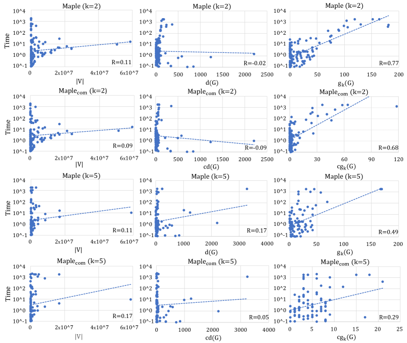
Figure 1: Scatter plots of the running time of Maple and Maple_com against the number of vertices $|V|$, the degeneracy values $d(G)$ and $cd(G)$, and the gap values $g_{k}(G)$ and $cg_{k}(G)$, for $k=2,5$.

In Table 4, we also present information on six representative graphs from the aforementioned datasets. We notice that, the degeneracy gap is often much smaller than the degeneracy. For example, $d(G)$ can be as large as 213 in soc-livejournal, while the $g_{k}(G)$ is only 1 when $k=2$. Indeed, our statistic result also reveals that $g_{k}(G)$ is often bounded by $O(\log{(|V|)})$ in most real-world graphs. On the flip side, the degeneracy gaps on artificial, dense graphs are large. When $k=2,5,10$, $g_{k}(G)$ of C125.9 is about $62$, $44$ and $21$, respectively. Consequently, our algorithm cannot solve these instances in a reasonable time. When $k=15$ and $20$, $g_{k}(G)$ of C125.9 is $5$ and $0$, respectively, and our algorithm can easily solve it in $66$ and $0$ seconds, respectively.

We also observed that the community-degeneracy $cd(G)$ is constantly smaller than the degeneracy $d(G)$ for all these instances. However, this does not hold for the community-degeneracy gap and the degeneracy gap. For small $k$ values like $2,5$, the community-degeneracy gap $cg_{k}(G)$ is usually smaller than the degeneracy gap $g_{k}(G)$. But as $k$ increases to $15$ or $20$, the community-degeneracy gap exceeds the degeneracy gap.

If we can compare the performance of our algorithms, Maple with the degeneracy ordering, Maple_com with the community-degeneracy ordering, and Maple_hyb with a hybrid mechanism. The results may vary depending on the scenario. In general, Maple outperforms Maple_hyb and shows a more robust performance than Maple_com.

Table 4: Properties and running behavior on six representative graphs. $T_{M}$, $T_{C}$, $T_{H}$, $T_{\overline{R}}$ and $T_{\overline{B}}$ stand for the running time of Maple, Maple_com, Maple_hyb, Maple_NGR and Maple_NBD respectively. $\gamma$ is the average branching factor of Maple.

Graph	$k$	$\omega_{k}(G)$	$g_{k}(G)$	$cg_{k}(G)$	$T_{M}$	$T_{C}$	$T_{H}$	$T_{\overline{R}}$	$T_{\overline{B}}$	$\gamma$
sc-pwtk $|V|=217891$ $|E|=5653221$ $d(G)=35$ $cd(G)=22$	2	24	13	2	2.18	8.78	3.64	3.88	2.24	2.00
	5	26	14	6	3.35	31.72	5.28	3.82	3.37	1.99
	10	33	12	9	10.43	144.63	12.05	10.80	10.57	2.00
	15	38	12	14	18.59	116.57	25.66	OOT	16.25	1.64
	20	46	9	16	6.22	61.78	84.10	18.20	6.23	1.97
soc-lastfm $|V|=1191805$ $|E|=4519330$ $d(G)=70$ $cd(G)=21$	2	18	54	7	13.66	3.32	2.97	16.94	14.20	1.30
	5	27	48	4	59.99	1.95	2.94	130.05	155.09	1.49
	10	38	42	3	2.25	1.83	1.58	OOT	2.26	1.43
	15	47	38	4	11.76	17.69	13.62	OOT	11.28	1.84
	20	56	34	5	1412.91	174.23	1476.13	OOT	1269.92	1.80
soc-livejournal $|V|=4033137$ $|E|=2193083$ $d(G)=213$ $cd(G)=212$	2	214	1	2	1.49	1.78	1.81	1.47	1.59	1.00
	5	214	4	8	1.78	2.46	2.26	1.83	1.90	1.00
	10	217	6	15	2.28	2.86	2.85	2.20	2.31	5.29
	15	221	7	21	1.55	1.91	1.66	1.54	1.64	1.00
	20	222	11	30	1.23	1.38	1.31	1.19	1.24	1.89
consph $|V|=79679$ $|E|=2963573$ $d(G)=41$ $cd(G)=22$	2	24	19	2	1.68	8.19	2.86	2.84	1.74	1.00
	5	26	20	6	24.80	45.23	15.65	14.71	24.87	1.89
	10	33	18	9	8.93	78.64	29.43	15.51	8.86	1.25
	15	42	14	10	16.68	87.12	21.00	91.69	16.19	1.45
	20	45	16	17	261.17	725.54	249.05	1621.17	233.18	1.84
C125.9 $|V|=125$ $|E|=6963$ $d(G)=102$ $cd(G)=84$	2	$\geq$ 42	$\leq$ 62	$\leq$ 46	OOT	OOT	OOT	OOT	OOT	OOT
	5	$\geq$ 63	$\leq$ 44	$\leq$ 31	OOT	OOT	OOT	OOT	OOT	OOT
	10	$\geq$ 91	$\leq$ 21	$\leq$ 13	OOT	OOT	OOT	OOT	OOT	OOT
	15	112	5	2	65.63	4.82	65.65	OOT	84.24	6.29
	20	122	0	2	0.00	0.00	0.00	0.00	0.00	1.00
MANN_a27 $|V|=378$ $|E|=70551$ $d(G)=364$ $cd(G)=350$	2	236	130	118	562.86	1299.49	609.94	609.33	OOT	2.22
	5	351	18	9	0.78	0.40	1.01	0.75	0.93	1.68
	10	351	23	19	266.10	213.03	269.07	18.74	OOT	2.25
	15	378	1	2	0.01	0.01	0.01	0.01	0.01	1.00
	20	378	6	12	0.01	0.01	0.01	0.01	0.01	1.00

5.2.2 Analysis on Graph Reduction.

To illustrate the effectiveness of our graph reduction, especially of the second- and higher-order reduction, the running time of Maple_NGR is also reported in Table 4, column $T_{\overline{R}}$. In general, graph reduction significantly improves practical performance. When $k=2,5$, graph reduction can achieve up to 2x speedup as shown on the soc-lastfm graph with $k=5$. When $k=10,15,20$, the benefit of graph reduction becomes more evident. For example, when $k=10$, Maple solves the soc-lastfm graph in 2.25s, while Maple_NGR fails to solve it within 1800s time limit. As another example, when $k=15$, Maple solves the sc-pwtk graph in 18.59s, while Maple_NGR still runs out of time. It is also worth noting that graph reduction does not always have a positive effect. For example, Maple takes 266.10s to solve the MANN_a27 graph, whereas Maple_NGR solves it with only 18.74s. The underlying reason is the computation overhead to perform the reduction rules.

5.2.3 Analysis on Bounding Technique.

To verify the effect of our bounding technique, especially for the minimum $d$-bdd size bound, the running time of Maple_NBD is also reported in Table 4, column $T_{\overline{B}}$. For the large real-world graphs from Network-Repo and 10th-DIMACS datasets, the effect of our bound is not as positive as our reduction rules. For example, due to computational overhead, although Maple outperforms Maple_NBD on the soc-lastfm graph when $k=5$, Maple is not as time-efficient as Maple_NBD on the soc-lastfm and consph graphs when $k=20$. But for artificial dense graphs from the 2nd-DIMACS benchmark, our bound proves to be very useful. For example, when $k=2$ and 10, Maple solves the MANN_a27 graph with 562.86s and 266.10s, respectively, whereas Maple_NBD fails to solve both of them. To sum up, our bound is more suitable for artificial dense graphs than real-world graphs.

5.2.4 Analysis on Branching Factor.

For a branching algorithm, the branching factor is defined as the number of sub-branches at each branch. In the worst case, the branching factor of DBDD subroutine is $k+1$. However, this worst-case estimation is pessimistic. In Table 4, we also show the average branching factor $\gamma$. In general, the average branching factor changes slightly as $k$ increases. In fact, it is always much smaller than $k+1$. We observe that when $k=2$, the branching factor on the consph and soc-livejournal graphs is $1.00$, meaning that an optimal solution can be found without branching. Even for C125.9, the branching factor $6.29$ is still much smaller than the worst-case value $16$, given $k=15$. The low value of the average branching factor is achieved by incorporating the aforementioned reduction rules and the bounding technique, which indicates that our algorithms run much faster than the worst-case estimation.

6 Conclusion and Perspective

In this paper, we presented new exact algorithms for the maximum $k$-plex problem and more importantly, we prvoided explanations of why these exponential-time algorithms can be efficient in practice. Our first algorithm is parameterized by the degeneracy gap $g_{k}(G)$, a parameter which is the difference between the degeneracy bound of graph $G$ and the size of the maximum $k$-plex in $G$. We extended our result with the community-degeneracy, which gives another algorithm parameterized by the community-degeneracy gap $cg_{k}(G)$, an even smaller parameter.

We showed in experiments that our algorithms are competitive with state-of-the-art algorithms. Then, we demonstrated that both the degeneracy gap and the community-degeneracy gap are very small in many real-world graphs, where our algorithms are very efficient. Finally, we conducted a correlation analysis to confirm the indicative function of gap parameters on the running time. Altogether, this work takes an important step towards bridging the gap between algorithmic complexity theory and practical efficiency in terms of running time.

This line of research can be extended from multiple perspectives. First, there should be more theoretical or empirical investigations between the multiple parameters and the running times. For example, one could build a systematic framework to incorporate all these parameters in one algorithm or include these graph parameters in an automatic run-time prediction tool. This has also been pointed out in the work of Figiel et al. (2022).

On the other hand, empirical fast algorithms with theoretical guarantees have been pursued for years in communities like operations research and artificial intelligence. This work provides novel insights into the use of parameterized complexity for solving hard graph problems. Specifically, graph parameters like degeneracy gaps can be extended and used in other graph models, like $k$-bundle (Zhou et al. 2022, Hu et al. 2023), $k$-defective clique (Chen et al. 2021, Gao et al. 2022) and so on.

Lastly, due to the importance of the $k$-plex model, our algorithm can be used or served as a subroutine in many other applications. For example, since the algorithm also works for the enumeration of maximal $k$-plexes, we can use this algorithm to accelerate the community detection task in (Conte et al. 2018, Zhu et al. 2020). The code of our algorithms that we make publicly available facilitates such applications.

Special thanks are given to Professor Christian Komusiewicz who introduced some important related works. This work was partially supported by CCF-Huawei Populus Grove Fund - Theoretical Computer Science Special Project, China Postdoctoral Science Foundation under grant 2022M722815, Natural Science Foundation of Sichuan Province of China under grants 2023NSFSC1415 and 2023NSFSC0059, and National Natural Science Foundation of China under grant 61972070.

7 Proofs

7.1 Proofs of Theorem 3.5

We have the following conclusion.

Lemma 7.1

Given a graph $G=(V,E)$, a fixed integer $k\geq 1$ and an integer $p$ that $p\geq 2k-1$, KPLEX_com$(G,k,p)$ solves the $k$-PLEX problem in time $O(|V|^{O(1)}(k+1)^{cg})$, where $cg=cd(G)+2k-p$.

Proof 7.2

Proof. Let $T_{KPLEX\mathrm{{}_{com}}}(G,k,p)$ denote the running time of KPLEX_com$(G,k,p)$. Then,

$$T_{KPLEX\mathrm{{}_{com}}}(G,k,p)=T_{commu}(G)+$$

$$\sum_{i=1}^{|E|}\sum_{\begin{subarray}{c}S\subseteq N^{2+}_{G}(e_{i})\\ |S|\leq 2k-2\end{subarray}}{\Bigl{(}T_{graph}(G_{s})+T_{DBDD}(\overline{G_{s}},k-1,t,N_{G}^{+}(e_{i}),\emptyset)\Bigr{)}},$$

where $T_{commu}(G)$ is the time of community-degeneracy ordering, $T_{graph}(G_{s})$ is the time of building $G_{s}$ given an edge $e_{i}=\{u,v\}$ and a subset $S$, and $T_{DBDD}(\overline{G_{s}},k-1,t,N_{G}^{+}(e_{i}),\emptyset)$ is the time of running DBDD$(\overline{G_{s}},k-1,t,N_{G}^{+}(e_{i}),\emptyset)$. Note that $G_{s}=(V_{s},E_{s})$ is the vertex-induced subgraph $G[\{u,v\}\cup S\cup N^{+}_{G}(e_{i})]$ and $t=|V_{s}|-p$.

It is known that $T_{commu}(G)\leq O(|V||E|)$ by Buchanan et al. (2014). Define $cg=cd(G)+2k-p$. Since $|N^{+}_{G}(e_{i})|\leq cd(G)$ and $|S|+2\leq 2k$, we have $|V_{s}|\leq cd(G)+|S|+2\leq cd(G)+2k$ and $t\leq cd(G)+2k-p=cg$. Therefore, $T_{graph}(G_{s})\leq(cd(G)+2k)^{2}$ and $T_{DBDD}(\overline{G_{s}},k-1,t,N_{G}^{+}(e_{i}),\emptyset)\leq(cd(G)+2k)^{2}(k+1)^{cg}$. Therefore,

$$T_{KPLEX\mathrm{{}_{com}}}(G,k,p)=O\biggl{(}|V||E|+$$

$$\sum_{i=1}^{|E|}\sum_{\begin{subarray}{c}S\subseteq N^{2+}_{G}(e_{i})\\ |S|\leq 2k-2\end{subarray}}{\Bigl{(}(cd(G)+2k)^{2}+(cd(G)+2k)^{2}(k+1)^{cg}\Bigr{)}}\biggr{)}$$

$$=O\biggl{(}|V||E|+\sum_{i=1}^{|E|}{|V|^{2k-2}(cd(G)+2k)^{2}(k+1)^{cg}}\biggr{)}$$

$$=O(|V||E|+|V|^{2k-1}(cd(G)+2k)^{2}(k+1)^{cg}).$$

which ends the proof.

Finally, for each $p$ starting from $|V|$ to $\omega_{k}(G)$, we run KPLEX_com$(G,k,p)$. At each time KPLEX is called, we have $cg\leq cd(G)+2k-\omega_{k}(G)$. Therefore, Theorem 3.5 holds.

7.2 Proof of Graph Reduction

Proof 7.3

Proof. Given a vertex set $P\subseteq V$, let $n=|P|$, $\lambda=|E(G[P])|$. Assume that $|\Delta_{G}(P)|<p-nk+n(n-1)-2\lambda$, but all vertices of $P$ belong to a $k$-plex $P^{*}$ of size at least $p$.

For any vertex $u\in P$, there are at most $k-(n-|N_{G}(u)\cap P|)$ vertices that are not adjacent to $u$ in $P^{*}\setminus P$. Hence, there are at most $\sum_{i=1}^{n}k-(n-|N_{G}(u_{i})\cap P|)$ vertices in $P^{*}\setminus P$ that are not belong to $\Delta_{G}(P)\cap P^{*}$. Then,

$$|P^{*}|-n-|\Delta_{G}(P)\cap P^{*}|\leq\sum_{i=1}^{n}k-(n-|N_{G}(u_{i})\cap P|)$$ (1)

$$=nk-n^{2}+\sum_{i=1}^{n}|N_{G}(u_{i})\cap P|=nk-n^{2}+2\lambda$$

In summary, we have $|\Delta_{G}(P)\cap P^{*}|\geq|P^{*}|-nk+n(n-1)-2\lambda\geq p-nk+n(n-1)-2\lambda$. It is clear that $|\Delta_{G}(P)\cap P^{*}|<=|\Delta_{G}(P)|$, which contradicts the assumption that $|\Delta_{G}(P)|<p-nk+n(n-1)-2\lambda$.

7.3 Proof of Lemma 4.1

Proof 7.4

Proof. Assuming that the vertices in $\pi_{0}$ form an independent set, it is obvious that this assumption will not increase the lower bound of the minimum $d$-bdd size. Thus we can move all vertices in $\pi_{0}$ from $C$ to $S$.

As $G[S]$ is $d$-degree bounded and $\pi_{i}$ is a subset of $v_{i}$’s neighbors in $C$, then at most $d-\delta_{i}$ vertices in $\pi_{i}$ can be included in $S$ at the same time. Hence, at most $\Sigma_{i=1}^{q}min\{d-\delta_{i},|\pi_{i}|\}$ vertices in $C\setminus\pi_{0}$ can be included in $S$.

To sum up, $|C|-|\pi_{0}|-\Sigma_{i=1}^{q}min\{d-\delta_{i},|\pi_{i}|\}$ is a lower bound of the minimum $d$-bdd excluding $S$ in $G$.

8 Missing Charts

Figure 2: Scatter graph of $d(G)$, $cd(G)$, $g_{k}(G)$ and $cg_{k}(G)$ for Network-Repo and 10th-DIMACS graphs, $k=2,5,10,15,20$. (Y-coordinate is cut off by 100 due to space limit.)

References

- Balasundaram et al. (2011) Balasundaram B, Butenko S, Hicks IV (2011) Clique relaxations in social network analysis: The maximum k-plex problem. Operations Research 59(1):133–142.
- Batagelj and Zaversnik (2003) Batagelj V, Zaversnik M (2003) An o(m) algorithm for cores decomposition of networks. arXiv preprint cs/0310049 .
- Buchanan et al. (2014) Buchanan A, Walteros JL, Butenko S, Pardalos PM (2014) Solving maximum clique in sparse graphs: an o (nm+ n2^ d/4) o (nm+ n 2 d/4) algorithm for d d-degenerate graphs. Optimization Letters 8:1611–1617.
- Chang et al. (2022) Chang L, Xu M, Strash D (2022) Efficient maximum k-plex computation over large sparse graphs. Proceedings of the VLDB Endowment 16(2):127–139.
- Chen et al. (2021) Chen X, Zhou Y, Hao JK, Xiao M (2021) Computing maximum k-defective cliques in massive graphs. Computers & Operations Research 127:105131.
- Conte et al. (2018) Conte A, De Matteis T, De Sensi D, Grossi R, Marino A, Versari L (2018) D2k: Scalable community detection in massive networks via small-diameter k-plexes. Proceedings of the 24th ACM SIGKDD International Conference on Knowledge Discovery & Data Mining, 1272–1281 (ACM).
- Cygan et al. (2015) Cygan M, Fomin FV, Kowalik Ł, Lokshtanov D, Marx D, Pilipczuk M, Pilipczuk M, Saurabh S (2015) Parameterized algorithms, volume 5 (Springer).
- Eppstein and Strash (2011) Eppstein D, Strash D (2011) Listing all maximal cliques in large sparse real-world graphs. International Symposium on Experimental Algorithms, 364–375 (Springer).
- Figiel et al. (2022) Figiel A, Koana T, Nichterlein A, Wünsche N (2022) Correlating theory and practice in finding clubs and plexes. arXiv preprint arXiv:2212.07533 .
- Gao et al. (2018) Gao J, Chen J, Yin M, Chen R, Wang Y (2018) An exact algorithm for maximum k-plexes in massive graphs. Proceedings of the 27th International Joint Conference on Artificial Intelligence, 1449–1455.
- Gao et al. (2022) Gao J, Xu Z, Li R, Yin M (2022) An exact algorithm with new upper bounds for the maximum k-defective clique problem in massive sparse graphs. Proceedings of the AAAI Conference on Artificial Intelligence, volume 36, 10174–10183.
- Gianinazzi et al. (2021) Gianinazzi L, Besta M, Schaffner Y, Hoefler T (2021) Parallel algorithms for finding large cliques in sparse graphs. Proceedings of the 33rd ACM Symposium on Parallelism in Algorithms and Architectures, 243–253.
- Gschwind et al. (2018) Gschwind T, Irnich S, Podlinski I (2018) Maximum weight relaxed cliques and russian doll search revisited. Discrete Applied Mathematics 234:131–138.
- Hooi et al. (2020) Hooi B, Shin K, Lamba H, Faloutsos C (2020) Telltail: Fast scoring and detection of dense subgraphs. Proceedings of the AAAI Conference on Artificial Intelligence, volume 34, 4150–4157.
- Hu et al. (2023) Hu S, Zhou Y, Xiao M, Fu ZH, Lü Z (2023) Listing maximal k-relaxed-vertex connected components from large graphs. Information Sciences 620:67–83.
- Jiang et al. (2021) Jiang H, Zhu D, Xie Z, Yao S, Fu ZH (2021) A new upper bound based on vertex partitioning for the maximum k-plex problem. Proceedings of the 30th International Joint Conference on Artificial Intelligence, 1689–1696.
- Khot and Raman (2002) Khot S, Raman V (2002) Parameterized complexity of finding subgraphs with hereditary properties. Theoretical Computer Science 289(2):997–1008.
- Komusiewicz (2016) Komusiewicz C (2016) Multivariate algorithmics for finding cohesive subnetworks. Algorithms 9(1):21.
- Komusiewicz et al. (2009) Komusiewicz C, Hüffner F, Moser H, Niedermeier R (2009) Isolation concepts for efficiently enumerating dense subgraphs. Theoretical Computer Science 410(38-40):3640–3654.
- Lund and Yannakakis (1993) Lund C, Yannakakis M (1993) The approximation of maximum subgraph problems. International Colloquium on Automata, Languages, and Programming, 40–51 (Springer).
- Matula and Beck (1983) Matula DW, Beck LL (1983) Smallest-last ordering and clustering and graph coloring algorithms. Journal of the ACM (JACM) 30(3):417–427.
- McClosky and Hicks (2012) McClosky B, Hicks IV (2012) Combinatorial algorithms for the maximum k-plex problem. Journal of Combinatorial Optimization 23(1):29–49.
- Moser et al. (2012) Moser H, Niedermeier R, Sorge M (2012) Exact combinatorial algorithms and experiments for finding maximum k-plexes. Journal of Combinatorial Optimization 24(3):347–373.
- Nishimura et al. (2005) Nishimura N, Ragde P, Thilikos DM (2005) Fast fixed-parameter tractable algorithms for nontrivial generalizations of vertex cover. Discrete Applied Mathematics 152(1-3):229–245.
- Nogueira and Pinheiro (2020) Nogueira B, Pinheiro RG (2020) A gpu based local search algorithm for the unweighted and weighted maximum s-plex problems. Annals of Operations Research 284(1):367–400.
- Pattillo et al. (2013) Pattillo J, Youssef N, Butenko S (2013) On clique relaxation models in network analysis. European Journal of Operational Research 226(1):9–18.
- Pattillo et al. (2012) Pattillo J, Youssef N, Butenko S, et al. (2012) Clique relaxation models in social network analysis. Springer Optimization and Its Applications 143–162.
- Pullan (2021) Pullan W (2021) Local search for the maximum k-plex problem. Journal of Heuristics 27(3):303–324.
- Seidman and Foster (1978) Seidman SB, Foster BL (1978) A graph-theoretic generalization of the clique concept. Journal of Mathematical Sociology 6(1):139–154.
- Shirokikh (2013) Shirokikh OA (2013) Degree-based Clique Relaxations: Theoretical Bounds, Computational Issues, and Applications. Ph.D. thesis, University of Florida.
- Tošić and Agha (2004) Tošić PT, Agha GA (2004) Maximal clique based distributed coalition formation for task allocation in large-scale multi-agent systems. International Workshop on Massively Multiagent Systems, 104–120 (Springer).
- Trukhanov et al. (2013a) Trukhanov S, Balasubramaniam C, Balasundaram B, Butenko S (2013a) Algorithms for detecting optimal hereditary structures in graphs, with application to clique relaxations. Computational Optimization and Applications 56(1):113–130, number: 1.
- Trukhanov et al. (2013b) Trukhanov S, Balasubramaniam C, Balasundaram B, Butenko S (2013b) Algorithms for detecting optimal hereditary structures in graphs, with application to clique relaxations. Computational Optimization and Applications 56(1):113–130.
- Walteros and Buchanan (2020) Walteros JL, Buchanan A (2020) Why is maximum clique often easy in practice? Operations Research 68(6):1866–1895.
- Wang et al. (2022) Wang Z, Zhou Y, Xiao M, Khoussainov B (2022) Listing maximal k-plexes in large real-world graphs. Proceedings of the ACM Web Conference 2022, 1517–1527.
- Wu and Hao (2015) Wu Q, Hao JK (2015) A review on algorithms for maximum clique problems. European Journal of Operational Research 242(3):693–709.
- Wünsche (2021) Wünsche N (2021) Mind the Gap When Searching for Relaxed Cliques. Master’s thesis, Technische Universität Berlin.
- Xiao (2016) Xiao M (2016) A parameterized algorithm for bounded-degree vertex deletion. Dinh TN, Thai MT, eds., Computing and Combinatorics - 22nd International Conference, COCOON 2016, Ho Chi Minh City, Vietnam, August 2-4, 2016, Proceedings, volume 9797 of Lecture Notes in Computer Science, 79–91 (Springer), URL http://dx.doi.org/10.1007/978-3-319-42634-1_7.
- Xiao et al. (2017) Xiao M, Lin W, Dai Y, Zeng Y (2017) A fast algorithm to compute maximum k-plexes in social network analysis. Proceedings of the AAAI conference on Artificial Intelligence, 919–925.
- Xiao and Nagamochi (2017) Xiao M, Nagamochi H (2017) Exact algorithms for maximum independent set. Information and Computation 255:126–146.
- Yannakakis (1978) Yannakakis M (1978) Node-and edge-deletion np-complete problems. Proceedings of the tenth annual ACM symposium on Theory of computing, 253–264 (ACM).
- Yu et al. (2006) Yu H, Paccanaro A, Trifonov V, Gerstein M (2006) Predicting interactions in protein networks by completing defective cliques. Bioinformatics 22(7):823–829.
- Zhou and Hao (2017) Zhou Y, Hao JK (2017) Frequency-driven tabu search for the maximum s-plex problem. Computers & Operations Research 86:65–78.
- Zhou et al. (2021) Zhou Y, Hu S, Xiao M, Fu ZH (2021) Improving maximum k-plex solver via second-order reduction and graph color bounding. Proceedings of the AAAI Conference on Artificial Intelligence, volume 35, 12453–12460.
- Zhou et al. (2022) Zhou Y, Lin W, Hao JK, Xiao M, Jin Y (2022) An effective branch-and-bound algorithm for the maximum s-bundle problem. European Journal of Operational Research 297(1):27–39.
- Zhou et al. (2020) Zhou Y, Xu J, Guo Z, Xiao M, Jin Y (2020) Enumerating maximal k-plexes with worst-case time guarantee. Proceedings of the AAAI conference on Artificial Intelligence, 2442–2449.
- Zhu et al. (2020) Zhu J, Chen B, Zeng Y (2020) Community detection based on modularity and k-plexes. Information Sciences 513:127–142.