V-line 2-tensor tomography in the plane

Abstract

In this article, we introduce and study various V-line transforms (VLTs) defined on symmetric $2$-tensor fields in $\mathbb{R}^{2}$. The operators of interest include the longitudinal, transverse, and mixed VLTs, their integral moments, and the star transform. With the exception of the star transform, all these operators are natural generalizations to the broken-ray trajectories of the corresponding well-studied concepts defined for straight-line paths of integration. We characterize the kernels of the VLTs and derive exact formulas for reconstruction of tensor fields from various combinations of these transforms. The star transform on tensor fields is an extension of the corresponding concepts that have been previously studied on vector fields and scalar fields (functions). We describe all injective configurations of the star transform on symmetric 2-tensor fields and derive an exact, closed-form inversion formula for that operator.

1 Introduction

The inverse problems of recovering a tensor field in $\mathbb{R}^{n}$ (or a Riemannian manifold) from various combinations of integral operators, such as the longitudinal, transverse, and momentum ray transforms applied to that field, have been studied extensively by various authors. In two-dimensional spaces (for both Euclidean and non-Euclidean settings) these questions have been addressed in the works [13, 24, 30, 31, 32] and in some of the references mentioned there. Numerous other studies have examined the injectivity, invertibility, and range characterization of the longitudinal ray transform and its moments in higher-dimensional Euclidean spaces (see [21, 22, 27, 28, 29, 33] and the references therein). Support theorems for integral moments of longitudinal geodesic ray transform and transverse geodesic ray transforms for symmetric $m$-tensor field defined on a Riemannian manifold have been studied in [1, 2]. The reconstruction problem for both the longitudinal and transverse ray transforms in $n$-dimensions ($n\geq 3$) is overdetermined, therefore one would like to have a reconstruction algorithm using only an $n$-dimensional restriction of the data. Such questions related to restricted data are also well-studied in different settings; for instance, see [11, 12, 23, 25, 35] and references therein. These problems, sometimes collectively called tomography of tensor fields, have applications in plasma physics, polarization imaging, prediction of earthquakes, and many other areas related to the propagation of radiation or waves through anisotropic media.

The transforms studied in the references mentioned above map a tensor field to various families of its integrals along straight lines (or geodesics). Physically, the operators integrating a tensor field (alternatively, a vector field or a function) along straight lines or rays often represent the ballistic regime of particle transport, describing the unimpeded flow of charged particles. At the same time, the mesoscopic regime of particle transport, allowing single-scattering events, leads to the consideration of operators integrating along broken-rays (also called V-lines) (e.g. see [14, 16, 17, 26]). The vertex of each V-line corresponds to a scattering location and, therefore, is inside the support of the image field. Generalized Radon-type transforms, mapping a scalar function to a family of its integrals along V-lines with a vertex inside the image support, have attracted substantial interest of researchers during the last two decades (see [4] and the references therein). Numerous interesting results have been obtained about the injectivity, range description, inversion, stability and other properties of the V-line transform, as well as the closely related star transform on scalar fields in $\mathbb{R}^{2}$ (see [3, 5, 6, 9, 10, 15, 19, 20, 34, 36, 37] and references therein).

The V-line and star transforms of vector fields in $\mathbb{R}^{2}$ have been analyzed in a pair of recent works [7, 8]. The authors extended the notions of the longitudinal, transverse, and momentum ray transforms from operators integrating vector fields along straight lines to those integrating along broken-ray trajectories. They described the kernels of these operators and derived several exact formulas for recovering a vector field from certain combinations of the aforementioned transforms. In addition to that, the notion of the star transform was extended from scalar fields (functions) to vector fields in $\mathbb{R}^{2}$, and an exact closed form inversion formula was derived for that operator. Building up on the previous results, the current work extends the notions of the V-line and star transforms to the symmetric 2-tensor fields in $\mathbb{R}^{2}$. We present explicit characterizations of the kernels of the VLTs and derive exact formulas for reconstruction of tensor fields from various combinations of those transforms. In addition to that, we describe all injective configurations of the star transform and derive an exact, closed-form inversion formula for that operator.

The paper is organized as follows. In Section 2, we define various V-line transforms on symmetric 2-tensor fields in $\mathbb{R}^{2}$, introduce the necessary notations, and prove some preliminary results. In Section 3, we characterize the kernels of the operators of our interest. In Section 4, we provide reconstruction results for some special kinds of tensor fields. In Section 5, we show the full reconstruction of a symmetric 2-tensor field from its longitudinal, transverse, and mixed V-line transforms. In Section 6, we demonstrate the full reconstruction of a symmetric 2-tensor field from the longitudinal, transverse and/or mixed V-line transforms combined with one of their first moment transforms. In Section 7, we introduce the star transform on symmetric 2-tensor fields in the plane and derive a closed-form inversion formula for that operator. Section 8 contains some additional remarks. We finish the paper with acknowledgements in Section 9.

2 Definitions, notations, and preliminary results

Throughout this paper, we use bold font letters to denote vectors and 2-tensors in $\mathbb{R}^{2}$ (e.g. x, u, v, f, etc.), and regular font letters to denote scalars (e.g. $x_{i}$, $h$, $f_{ij}$, etc). We denote by $\textbf{{x}}\cdot\textbf{{y}}$ the usual dot product between vectors x and y.

Let $S^{2}(\Omega)$ denote the space of symmetric $2$-tensor fields defined in a domain $\Omega\subseteq\mathbb{R}^{2}$, and $C_{c}^{2}\left(S^{2};\Omega\right)$ be the space of twice continuously differentiable, compactly supported, symmetric $2$-tensor fields. In local coordinates, $\textbf{{f}}\in C_{c}^{2}\left(S^{2};\Omega\right)$ can be expressed as

$$\textbf{{f}}(x)=f_{ij}(x)\,dx^{i}dx^{j},$$ (1)

where $f_{ij}(x)$ are compactly supported $C^{2}$ functions such that $f_{ij}=f_{ji}$ for all indices $i$ and $j$. The Einstein summation convention is assumed throughout the article.

The scalar product in $S^{2}(\Omega)$ is defined by the formula

$$\langle\textbf{{f}},\textbf{{g}}\rangle=f_{ij}g^{ij}=f_{11}g^{11}+2f_{12}g^{12}+f_{22}g^{22}.$$ (2)

For a scalar function $V(x_{1},x_{2})$ and a vector field $\textbf{{f}}=(f_{1},f_{2})$, we use the notations

$$\mathrm{d}V=\left(\frac{\partial V}{\partial x_{1}},\frac{\partial V}{\partial x_{2}}\right),\ \ \mathrm{d}^{\perp}V=\left(-\frac{\partial V}{\partial x_{2}},\frac{\partial V}{\partial x_{1}}\right),\ \ \delta\textbf{{f}}=\frac{\partial f_{1}}{\partial x_{1}}+\frac{\partial f_{2}}{\partial x_{2}},\ \ \delta^{\perp}\textbf{{f}}=\frac{\partial f_{2}}{\partial x_{1}}-\frac{\partial f_{1}}{\partial x_{2}}.$$ (3)

The operators $\mathrm{d}$ and $\delta$ are the classical gradient and divergence operators, respectively, while the operators $\mathrm{d}^{\perp}$ and $\delta^{\perp}$ are the corresponding “orthogonal” operators. These operators can be generalized naturally to higher-order tensor fields in the following way:

$$(\mathrm{d}\textbf{{f}})_{ij} =\frac{1}{2}\left(\frac{\partial f_{i}}{\partial x_{j}}+\frac{\partial f_{j}}{\partial x_{i}}\right),\quad\textbf{{f}}\mbox{ is a vector field,}$$ (4)

$$(\mathrm{d}^{\perp}\textbf{{f}})_{ij} =\frac{1}{2}\left((-1)^{j}\frac{\partial f_{i}}{\partial x_{3-j}}+(-1)^{i}\frac{\partial f_{j}}{\partial x_{3-i}}\right),\quad\textbf{{f}}\mbox{ is a vector field,}$$ (5)

$$(\delta\textbf{{f}})_{i} =\frac{f_{i1}}{\partial x_{1}}+\frac{f_{i2}}{\partial x_{2}}=\frac{f_{ij}}{\partial x_{j}},\quad\textbf{{f}}\mbox{ is a symmetric 2-tensor field,}$$ (6)

$$(\delta^{\perp}\textbf{{f}})_{i} =-\frac{f_{i1}}{\partial x_{2}}+\frac{f_{i2}}{\partial x_{1}}=(-1)^{j}\frac{f_{ij}}{\partial x_{3-j}},\quad\textbf{{f}}\mbox{ is a symmetric 2-tensor field.}$$ (7)

Remark 1.

The generalized operators $\mathrm{d}$ and $\delta$ defined above are known as symmetrized derivative/inner differentiation and divergence on tensor fields, respectively (e.g., see [33, p. 25]).

Let u and v be two linearly independent unit vectors in $\mathbb{R}^{2}$. For $\textbf{{x}}\in\mathbb{R}^{2}$, the rays emanating from x in directions u and v are denoted by $L_{\textbf{{u}}}(\textbf{{x}})$ and $L_{\textbf{{v}}}(\textbf{{x}})$ respectively, i.e.

$$L_{\textbf{{u}}}(\textbf{{x}})=\left\{\textbf{{x}}+t\textbf{{u}}:0\leq t<\infty\right\}\quad\mbox{ and }\quad L_{\textbf{{v}}}(\textbf{{x}})=\left\{\textbf{{x}}+t\textbf{{v}}:0\leq t<\infty\right\}.$$

A V-line with the vertex x is the union of rays $L_{\textbf{{u}}}(\textbf{{x}})$ and $L_{\textbf{{v}}}(\textbf{{x}})$. Through the rest of the article we will assume that u and v are fixed, i.e. all V-lines have the same ray directions and can be parametrized simply by the coordinates x of the vertex (see Figure 1(a)).

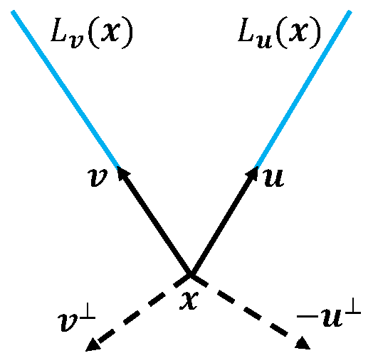
(a) A V-line with vertex at x, ray directions u, v and outward normals $-\textbf{{u}}^{\perp}$, $\textbf{{v}}^{\perp}$.

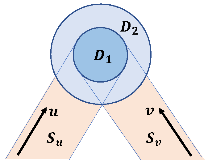
(b) A sketch of the compact support of f and the unbounded support of $\mathcal{L}\textbf{{f}}$, $\mathcal{T}\textbf{{f}}$, $\mathcal{M}\textbf{{f}}$.

Figure 1: From [7].

Definition 1.

The divergent beam transform $\mathcal{X}_{\textbf{{u}}}$ of function $h$ at $\textbf{{x}}\in\mathbb{R}^{2}$ in the direction $\textbf{{u}}\in\mathbb{S}^{1}$ is defined as:

$$\mathcal{X}_{\textbf{{u}}}h(\textbf{{x}})=\int_{0}^{\infty}h(\textbf{{x}}+t\textbf{{u}})\,dt.$$ (8)

Definition 2.

Let $k\geq 0$ be in an integer. The $k$-th moment divergent beam transform of a function $h$ in the direction $\textbf{{u}}\in\mathbb{S}^{1}$ is defined as follows

$$\mathcal{X}^{k}_{\textbf{{u}}}h=\int_{0}^{\infty}h(\textbf{{x}}+t\textbf{{u}})\,t^{k}\,dt.$$ (9)

The directional derivative of a function in the direction u is denoted by $D_{\textbf{{u}}}$, i.e.

$$D_{\textbf{{u}}}h=\textbf{{u}}\cdot\nabla h.$$ (10)

For a compactly supported function $h$, the operators $\mathcal{X}_{\textbf{{u}}}$ and $D_{\textbf{{u}}}$ commute and satisfy the following relation:

$$\mathcal{X}_{\textbf{{u}}}(D_{\textbf{{u}}}h)(\textbf{{x}})=D_{\textbf{{u}}}(\mathcal{X}_{\textbf{{u}}}h)(\textbf{{x}})=-h(\textbf{{x}}).$$ (11)

Definition 3.

For two vectors $\textbf{{u}}=(u_{1},u_{2})$ and $\textbf{{v}}=(v_{1},v_{2})$, the tensor product $\textbf{{u}}\otimes\textbf{{v}}$ is a rank-2 tensor with its $ij$-th component defined by

$$(\textbf{{u}}\otimes\textbf{{v}})_{ij}=u_{i}v_{j}.$$ (12)

The symmetrized tensor product $\textbf{{u}}\odot\textbf{{v}}$ is then defined as

$$\textbf{{u}}\odot\textbf{{v}}=\frac{1}{2}\left(\textbf{{u}}\otimes\textbf{{v}}+\textbf{{v}}\otimes\textbf{{u}}\right).$$ (13)

We use the notation $\textbf{{u}}^{2}$ for the tensor (symmetrized) product of a vector u with itself, that is,

$$\textbf{{u}}^{2}=\textbf{{u}}\odot\textbf{{u}}=\textbf{{u}}\otimes\textbf{{u}}.$$

In this paper, our main goal is to recover a symmetric 2-tensor field from its V-line transforms, which we define below.

Definition 4.

Let $\textbf{{f}}\in C_{c}^{2}\left(S^{2};\mathbb{R}^{2}\right)$. The longitudinal V-line transform of f is defined as

$$\mathcal{L}_{\textbf{{u}},\textbf{{v}}}\,\textbf{{f}}\ =\mathcal{X}_{\textbf{{u}}}\left(\left\langle\textbf{{f}},\textbf{{u}}^{2}\right\rangle\right)+\mathcal{X}_{\textbf{{v}}}\left(\left\langle\textbf{{f}},\textbf{{v}}^{2}\right\rangle\right).$$ (14)

To define the second integral transform of interest, we need to make a choice for the normal unit vectors corresponding to each branch of the V-line. We define the vector $\perp$ operation by $(x_{1},x_{2})^{\perp}=(-x_{2},x_{1})$.

Definition 5.

Let $\textbf{{f}}\in C_{c}^{2}\left(S^{2};\mathbb{R}^{2}\right)$. The transverse V-line transform of f is defined as

$$\mathcal{T}_{\textbf{{u}},\textbf{{v}}}\,\textbf{{f}}\ =\mathcal{X}_{\textbf{{u}}}\left(\left\langle\textbf{{f}},(\textbf{{u}}^{\perp})^{2}\right\rangle\right)+\mathcal{X}_{\textbf{{v}}}\left(\left\langle\textbf{{f}},(\textbf{{v}}^{\perp})^{2}\right\rangle\right).$$ (15)

Definition 6.

Let $\textbf{{f}}\in C_{c}^{2}\left(S^{2};\mathbb{R}^{2}\right)$. The mixed V-line transform of f is defined as

$$\mathcal{M}_{\textbf{{u}},\textbf{{v}}}\,\textbf{{f}}\ =\mathcal{X}_{\textbf{{u}}}\left(\left\langle\textbf{{f}},\textbf{{u}}\odot\textbf{{u}}^{\perp}\right\rangle\right)+\mathcal{X}_{\textbf{{v}}}\left(\left\langle\textbf{{f}},\textbf{{v}}\odot\textbf{{v}}^{\perp}\right\rangle\right).$$ (16)

Definition 7.

Let $\textbf{{f}}\in C_{c}^{2}\left(S^{2};\mathbb{R}^{2}\right)$. The $k$-th moment longitudinal V-line transform of f is defined as

$$\mathcal{L}^{k}_{\textbf{{u}},\textbf{{v}}}\,\textbf{{f}}\ =\mathcal{X}^{k}_{\textbf{{u}}}\left(\left\langle\textbf{{f}},\textbf{{u}}^{2}\right\rangle\right)+\mathcal{X}^{k}_{\textbf{{v}}}\left(\left\langle\textbf{{f}},\textbf{{v}}^{2}\right\rangle\right).$$ (17)

Definition 8.

Let $\textbf{{f}}\in C_{c}^{2}\left(S^{2};\mathbb{R}^{2}\right)$. The $k$-th moment transverse V-line transform of f is defined as

$$\mathcal{T}^{k}_{\textbf{{u}},\textbf{{v}}}\,\textbf{{f}}\ =\mathcal{X}^{k}_{\textbf{{u}}}\left(\left\langle\textbf{{f}},(\textbf{{u}}^{\perp})^{2}\right\rangle\right)+\mathcal{X}^{k}_{\textbf{{v}}}\left(\left\langle\textbf{{f}},(\textbf{{v}}^{\perp})^{2}\right\rangle\right).$$ (18)

Definition 9.

Let $\textbf{{f}}\in C_{c}^{2}\left(S^{2};\mathbb{R}^{2}\right)$. The $k$-th moment mixed V-line transform of f is defined as

$$\mathcal{M}^{k}_{\textbf{{u}},\textbf{{v}}}\,\textbf{{f}}\ =\mathcal{X}^{k}_{\textbf{{u}}}\left(\left\langle\textbf{{f}},\textbf{{u}}\odot\textbf{{u}}^{\perp}\right\rangle\right)+\mathcal{X}^{k}_{\textbf{{v}}}\left(\left\langle\textbf{{f}},\textbf{{v}}\odot\textbf{{v}}^{\perp}\right\rangle\right).$$ (19)

Remark 2.

Throughout the paper we assume that the linearly independent unit vectors u and v are fixed. Hence, to simplify the notations, we will drop the indices $\textbf{{u}},\textbf{{v}}$ and refer to $\mathcal{T}_{\textbf{{u}},\textbf{{v}}}$, $\mathcal{L}_{\textbf{{u}},\textbf{{v}}}$, $\mathcal{M}_{\textbf{{u}},\textbf{{v}}}$, $\mathcal{T}^{k}_{\textbf{{u}},\textbf{{v}}}$, $\mathcal{L}^{k}_{\textbf{{u}},\textbf{{v}}}$, and $\mathcal{M}^{k}_{\textbf{{u}},\textbf{{v}}}$ simply as $\mathcal{T}$, $\mathcal{L}$, $\mathcal{M}$, $\mathcal{T}^{k}$, $\mathcal{L}^{k}$, and $\mathcal{M}^{k}$.

Let us assume that $\operatorname{supp}\textbf{{f}}\subseteq D_{1}$, where $D_{1}$ is an open disc of radius $r_{1}$ centered at the origin. Then $\mathcal{T}\textbf{{f}}$, $\mathcal{L}\textbf{{f}}$, $\mathcal{M}\textbf{{f}}$, and their moments are supported inside an unbounded domain $D_{2}\cup S_{\textbf{{u}}}\cup S_{\textbf{{v}}}$, where $D_{2}$ is a disc of some finite radius $r_{2}>r_{1}$ centered at the origin, while $S_{\textbf{{u}}}$ and $S_{\textbf{{v}}}$ are semi-infinite strips (outside of $D_{2}$) in the direction of u and v, respectively (see Figure 1(b)). It is easy to notice that $\mathcal{L}\textbf{{f}},\mathcal{T}\textbf{{f}}$, and $\mathcal{M}\textbf{{f}}$ are constant along the rays in the directions u and v inside the corresponding strips $S_{\textbf{{u}}}$ and $S_{\textbf{{v}}}$. In other words, their restrictions to $\overline{D_{2}}$ completely define them in $\mathbb{R}^{2}$. If one also knows the corresponding moments in $\overline{D_{2}}$, then the values of the moments are uniquely determined everywhere else. Indeed, let y be inside the strip $S_{\textbf{{u}}}$, and x be a point on the boundary between $D_{2}$ and $S_{\textbf{{u}}}$ such that $\textbf{{y}}+a\textbf{{u}}=\textbf{{x}}$ for some constant $a\textgreater 0$. It is easy to see that

$$\mathcal{L}^{1}\textbf{{f}}(\textbf{{y}})=\mathcal{L}^{1}\textbf{{f}}(\textbf{{x}})+a\mathcal{L}\textbf{{f}}(\textbf{{x}}).$$ (20)

Similar result follows for transverse and mixed moment V-line transforms.

Remark 3.

In this article we assume that the tensor field f is supported in $D_{1}$ and the transforms $\mathcal{L}\textbf{{f}}\,(\textbf{{x}})$, $\mathcal{T}\textbf{{f}}\,(\textbf{{x}})$, $\mathcal{M}\textbf{{f}}\,{(\textbf{{x}})}$, and their moments are known for all $\textbf{{x}}\in\overline{D_{2}}$.

Remark 4.

To simplify various calculations, we assume $\textbf{{u}}=(u_{1},u_{2})$ and $\textbf{{v}}=(-u_{1},u_{2})$, that is, the V-lines are symmetric with respect to the $y$-axis. This choice does not change the analysis of the general case, since the data obtained in one setup of u and v can be transformed into the data obtained for the other setup and vice versa.

Remark 5.

If $\textbf{{u}}=(0,1)=\textbf{{v}}$, the V-line degenerates into a pair of coinciding rays. If $\textbf{{u}}=(1,0)=-\textbf{{v}}$, the V-line becomes a straight line. Since we are interested in proper V-lines, we avoid both of these extreme cases. Therefore, we assume $-1<u_{1}^{2}-u_{2}^{2}<1$.

With this choice of the parameters of the V-lines, we have the following identities (which can be verified by direct calculations):

$$\langle\textbf{{f}},\textbf{{u}}^{2}\rangle =u_{1}^{2}f_{11}+2u_{1}u_{2}f_{12}+u_{2}^{2}f_{22},$$

$$\langle\textbf{{f}},\textbf{{u}}_{\perp}^{2}\rangle =u_{2}^{2}f_{11}-2u_{1}u_{2}f_{12}+u_{1}^{2}f_{22},$$

$$\langle\textbf{{f}},\textbf{{u}}\odot\textbf{{u}}_{\perp}\rangle =-u_{1}u_{2}f_{11}+(u_{1}^{2}-u_{2}^{2})f_{12}+u_{1}u_{2}f_{22},$$

$$\langle\textbf{{f}},\textbf{{v}}^{2}\rangle =u_{1}^{2}f_{11}-2u_{1}u_{2}f_{12}+u_{2}^{2}f_{22},$$

$$\langle\textbf{{f}},\textbf{{v}}_{\perp}^{2}\rangle =u_{2}^{2}f_{11}+2u_{1}u_{2}f_{12}+u_{1}^{2}f_{22},$$

$$\langle\textbf{{f}},\textbf{{v}}\odot\textbf{{v}}_{\perp}\rangle =u_{1}u_{2}f_{11}+(u_{1}^{2}-u_{2}^{2})f_{12}-u_{1}u_{2}f_{22}.$$

Using these identities, we can rewrite our integral operators in the following simplified forms:

$$\mathcal{L}\textbf{{f}}(\textbf{{x}}) =u_{1}^{2}\mathcal{V}(f_{11})(\textbf{{x}})+2u_{1}u_{2}\mathcal{V}^{-}(f_{12})(\textbf{{x}})+u_{2}^{2}\mathcal{V}(f_{22})(\textbf{{x}}),$$ (21)

$$\mathcal{T}\textbf{{f}}(\textbf{{x}}) =u_{2}^{2}\mathcal{V}(f_{11})(\textbf{{x}})-2u_{1}u_{2}\mathcal{V}^{-}(f_{12})(\textbf{{x}})+u_{1}^{2}\mathcal{V}(f_{22})(\textbf{{x}}),$$ (22)

$$\mathcal{M}\textbf{{f}}(\textbf{{x}}) =-u_{1}u_{2}\mathcal{V}^{-}(f_{11})(\textbf{{x}})+(u_{1}^{2}-u^{2}_{2})\mathcal{V}(f_{12})(\textbf{{x}})+u_{1}u_{2}\mathcal{V}^{-}(f_{22})(\textbf{{x}}),$$ (23)

where $\mathcal{V}\varphi$ and $\mathcal{V}^{-}\varphi$ denote the V-line transform and the signed V-line transform of scalar function $\varphi$. Namely,

$$\mathcal{V}\varphi(\textbf{{x}})=\mathcal{X}_{\textbf{{u}}}\varphi(\textbf{{x}})+\mathcal{X}_{\textbf{{v}}}\varphi(\textbf{{x}}),$$ (24)

and

$$\mathcal{V}^{-}\varphi(\textbf{{x}})=\mathcal{X}_{\textbf{{u}}}\varphi(\textbf{{x}})-\mathcal{X}_{\textbf{{v}}}\varphi(\textbf{{x}}).$$ (25)

Theorem 1.

Let $\textbf{{f}}\in C_{c}^{2}\left(S^{2};D_{1}\right)$. Then the knowledge of $\mathcal{L}\textbf{{f}}$ and $\mathcal{T}\textbf{{f}}$ determines the trace of f as follows:

$$\left(f_{11}+f_{22}\right)(\textbf{{x}})=\frac{1}{2u_{2}}D_{\textbf{{u}}}D_{\textbf{{v}}}\int_{0}^{\infty}\left(\mathcal{L}\textbf{{f}}+\mathcal{T}\textbf{{f}}\right)(\textbf{{x}}+t\textbf{{e}}_{2})\,dt,$$ (26)

where $\textbf{{e}}_{2}=(0,1)$.

Proof.

By adding equations (21) and (22), we get the following relation:

$$\mathcal{L}\textbf{{f}}(\textbf{{x}})+\mathcal{T}\textbf{{f}}(\textbf{{x}})=\mathcal{V}\left(f_{11}+f_{22}\right)(\textbf{{x}}).$$

Using the inversion of the V-line transform given in [5, Corollary 2], we obtain the required inversion formula (26). ∎

One can easily observe that, when the branches of the V-lines are orthogonal to each other (or, equivalently, when $u_{1}=u_{2}$), the symmetric tensor products $\textbf{{u}}^{2}$, $\textbf{{u}}_{\perp}^{2}$, $\textbf{{u}}\odot\textbf{{u}}_{\perp}$, $\textbf{{v}}^{2}$, $\textbf{{v}}_{\perp}^{2}$, and $\textbf{{v}}\odot\textbf{{v}}_{\perp}$ become degenerate. As it will be shown throughout the paper, this special case exhibits a qualitatively different behaviour in the problems of recovering f from its integral transforms. For example, the results of Theorem 1, in that particular setup, can be augmented as follows.

Theorem 2.

Let $\textbf{{f}}\in C_{c}^{2}\left(S^{2};D_{1}\right)$ and $u_{1}=u_{2}$. The knowledge of $\mathcal{L}\textbf{{f}}$ and $\mathcal{T}\textbf{{f}}$ determines the off-diagonal component $f_{12}$ of f as follows:

$$f_{12}(\textbf{{x}})=\frac{1}{4u_{1}}D_{\textbf{{u}}}D_{\textbf{{v}}}\int_{0}^{\infty}\left(\mathcal{L}\textbf{{f}}-\mathcal{T}\textbf{{f}}\right)(\textbf{{x}}-t\textbf{{e}}_{1})\,dt,$$ (27)

where $\textbf{{e}}_{1}=(1,0)$, while $\mathcal{M}\textbf{{f}}$ provides the difference of the diagonal components of f through:

$$\left(f_{22}-f_{11}\right)(\textbf{{x}})=\frac{1}{u_{1}}D_{\textbf{{u}}}D_{\textbf{{v}}}\int_{0}^{\infty}\mathcal{M}\textbf{{f}}\,(\textbf{{x}}-t\textbf{{e}}_{1})\,dt.$$ (28)

Proof.

By subtracting equation (22) from equation (21), we get the following relation:

$$\mathcal{L}\textbf{{f}}(\textbf{{x}})-\mathcal{T}\textbf{{f}}(\textbf{{x}})=4u_{1}^{2}\,\mathcal{V}^{-}f_{12}(\textbf{{x}}).$$

Under the assumption $u_{1}=u_{2}$, equation (23) simplifies into the expression:

$$\mathcal{M}\textbf{{f}}(\textbf{{x}})=u_{1}^{2}\;\mathcal{V}^{-}(f_{22}-f_{11})(\textbf{{x}}).$$

Using the inversion of the signed V-line transform given in [5, Theorem 7], we obtain both of the required inversion formulas (27) and (28). ∎

Corollary 1.

If $u_{1}=u_{2}$, then $\textbf{{f}}\in C_{c}^{2}\left(S^{2};D_{1}\right)$ can be recovered from $\mathcal{L}\textbf{{f}}$, $\mathcal{T}\textbf{{f}}$, and $\mathcal{M}\textbf{{f}}$.

3 Kernel descriptions of transforms $\mathcal{L}$, $\mathcal{T}$, and $\mathcal{M}$

This section is devoted to the study of the kernels of the VLTs defined on $C_{c}^{2}\left(S^{2};\mathbb{R}^{2}\right)$. Each of these integral transforms has a non-trivial null space, which we characterize below. Our findings here are quite different from the known results for the usual straight-line transforms. For instance, the potential tensor fields are in the kernel of the longitudinal ray transform (along straight lines) [33], which is not the case in the V-line setup, as one can easily check.

Theorem 3.

Let $\textbf{{f}}\in C_{c}^{2}\left(S^{2};D_{1}\right)$. Then

1. f is in the kernel of $\mathcal{L}$ if and only if there exists a scalar function $\varphi$ such that

   $$\mathrm{d}\varphi=\left(u_{1}^{2}f_{11}+u_{2}^{2}f_{22},2u_{1}^{2}f_{12}\right).$$ (29)

2. f is in the kernel of $\mathcal{T}$ if and only if there exists a scalar function $\varphi$ such that

   $$\mathrm{d}\varphi=\left(u_{2}^{2}f_{11}+u_{1}^{2}f_{22},-2u_{1}^{2}f_{12}\right).$$ (30)

3. f is in the kernel of $\mathcal{M}$ if and only if there exists a scalar function $\varphi$ such that

   $$\mathrm{d}\varphi=\left((u_{1}^{2}-u_{2}^{2})f_{12},-u_{1}^{2}(f_{11}-f_{22})\right).$$ (31)

Proof.

Part (a). As a first step, we observe that $\mathcal{L}\textbf{{f}}(\textbf{{x}})=0$ if and only if $D_{\textbf{{u}}}D_{\textbf{{v}}}\mathcal{L}\textbf{{f}}(\textbf{{x}})=0$. This follows from formula (11) after applying $\mathcal{X}_{\textbf{{v}}}\mathcal{X}_{\textbf{{u}}}$ to the second relation. Now, consider

$$D_{\textbf{{u}}}D_{\textbf{{v}}}\mathcal{L}\textbf{{f}}=0 \Longleftrightarrow 4u_{1}^{2}u_{2}\partial_{x_{1}}f_{12}-2u_{1}^{2}u_{2}\partial_{x_{2}}f_{11}-2u_{2}^{3}\partial_{x_{2}}f_{22}=0$$

$$\Longleftrightarrow\operatorname{curl}\left(u_{1}^{2}f_{11}+u_{2}^{2}f_{22},2u_{1}^{2}f_{12}\right)=0.$$

It is known that $\operatorname{curl}(\textbf{{g}})=\partial_{x_{1}}g_{2}-\partial_{x_{2}}g_{1}$ of a 2D vector field g vanishes if and only if $\textbf{{g}}=\mathrm{d}\varphi$ for some scalar function $\varphi$. Therefore, there exists a scalar function $\varphi$ such that

$$\mathrm{d}\varphi=\left(u_{1}^{2}f_{11}+u_{2}^{2}f_{22},2u_{1}^{2}f_{12}\right).$$

Part (b). Proceeding as in the previous part, observe that $\mathcal{T}\textbf{{f}}(\textbf{{x}})=0$ iff $-D_{\textbf{{u}}}D_{\textbf{{v}}}\mathcal{T}\textbf{{f}}(\textbf{{x}})=0$.

$$-D_{\textbf{{u}}}D_{\textbf{{v}}}\mathcal{T}\textbf{{f}}=0 \Longleftrightarrow 4u_{1}^{2}u_{2}\partial_{x_{1}}f_{12}+2u_{2}^{3}\partial_{x_{2}}f_{11}+2u_{1}^{2}u_{2}\partial_{x_{2}}f_{22}=0$$

$$\Longleftrightarrow\operatorname{div}\left(2u_{1}^{2}f_{12},u_{2}^{2}f_{11}+u_{1}^{2}f_{22}\right)=0{\color[rgb]{0,0,1}{.}}$$ (32)

For every two-dimensional solenoidal vector field g on the unit disk, there exists a scalar function $\varphi$ such that $\textbf{{g}}=\mathrm{d}^{\perp}\varphi.$ Hence, f is in the kernel of $\mathcal{T}$ if and only if there exists a $\varphi$ such that

$$\mathrm{d}^{\perp}\varphi=\left(2u_{1}^{2}f_{12},u_{2}^{2}f_{11}+u_{1}^{2}f_{22}\right)\Longleftrightarrow\mathrm{d}\varphi=\left(u_{2}^{2}f_{11}+u_{1}^{2}f_{22},-2u_{1}^{2}f_{12}\right).$$

Part (c). Again, note that $\mathcal{M}\textbf{{f}}(\textbf{{x}})=0$ if and only if $-D_{\textbf{{u}}}D_{\textbf{{v}}}\mathcal{M}\textbf{{f}}(\textbf{{x}})=0$. Then

$$-D_{\textbf{{u}}}D_{\textbf{{v}}}\mathcal{M}\textbf{{f}}=0 \Longleftrightarrow 2u_{1}^{2}u_{2}\partial_{x_{1}}f_{11}-2u_{1}^{2}u_{2}\partial_{x_{1}}f_{22}+2u_{2}(u_{1}^{2}-u_{2}^{2})\partial_{x_{2}}f_{12}=0$$

$$\Longleftrightarrow\operatorname{div}\left(u_{1}^{2}\left(f_{11}-f_{22}\right),\left(u_{1}^{2}-u_{2}^{2}\right)f_{12}\right)=0.$$

Therefore, f is in the kernel of $\mathcal{M}$ if and only if there exists a scalar function $\varphi$ such that

$$\mathrm{d}^{\perp}\varphi=\left(u_{1}^{2}\left(f_{11}-f_{22}\right),\left(u_{1}^{2}-u_{2}^{2}\right)f_{12}\right)\Longleftrightarrow\mathrm{d}\varphi=\left(\left(u_{1}^{2}-u_{2}^{2}\right)f_{12},-u_{1}^{2}\left(f_{11}-f_{22}\right)\right),$$

which finishes the proof. ∎

4 Reconstruction results for special kinds of tensor fields

In this section we focus on symmetric 2-tensor fields of the form $\mathrm{d}\textbf{{g}}$ or $\mathrm{d}^{\perp}\textbf{{g}}$, where g is a vector field in $\mathbb{R}^{2}$. We show that such tensor fields can be recovered from the knowledge of specific combinations of their VLTs. Furthermore, if the unknown tensor field is of the form $\mathrm{d}^{2}\varphi$, $\mathrm{d}\mathrm{d}^{\perp}\varphi$ or $(\mathrm{d}^{\perp})^{2}\varphi$, where $\varphi$ is a scalar function, then the field can be uniquely reconstructed just from one integral transform, depending on the form of f.

Theorem 4.

Let $\textbf{{g}}=(g_{1},g_{2})$ be a vector field with components $g_{i}(\textbf{{x}})\in C_{c}^{2}(D_{1})$, for $i=1,2$.

• If f is a symmetric 2-tensor field of the form $\textbf{{f}}=\mathrm{d}\textbf{{g}}$, then it can be recovered explicitly in terms of $\mathcal{L}\textbf{{f}}$ and $\mathcal{M}\textbf{{f}}$.

• If f is a symmetric 2-tensor field of the form $\textbf{{f}}=\mathrm{d}^{\perp}\textbf{{g}}$, then it can be recovered explicitly in terms of $\mathcal{T}\textbf{{f}}$ and $\mathcal{M}\textbf{{f}}$.

Proof.

Part (a). From the definition of the symmetrized derivative (4), we have

$$f_{ij}=(\mathrm{d}\textbf{{g}})_{ij}=\frac{1}{2}\left(\frac{\partial g_{i}}{\partial x_{j}}+\frac{\partial g_{j}}{\partial x_{i}}\right).$$

A direct computation yields

$$\int_{0}^{\infty}f_{ij}(\textbf{{x}}+t\textbf{{u}})u^{i}u^{j}\,dt=\frac{1}{2}\int_{0}^{\infty}\left(\frac{\partial g_{i}}{\partial x_{j}}+\frac{\partial g_{j}}{\partial x_{i}}\right)(\textbf{{x}}+t\textbf{{u}})u^{i}u^{j}\,dt=-\left\langle\textbf{{g}}(\textbf{{x}}),\textbf{{u}}\right\rangle,$$ (33)

$$\int_{0}^{\infty}f_{ij}(\textbf{{x}}+t\textbf{{u}})u^{i}(u^{\perp})^{j}\,dt =\frac{1}{2}\int_{0}^{\infty}\left(\frac{\partial g_{i}}{\partial x_{j}}+\frac{\partial g_{j}}{\partial x_{i}}\right)(\textbf{{x}}+t\textbf{{u}})u^{i}(u^{\perp})^{j}\,dt$$

$$=-\left\langle\textbf{{g}}(\textbf{{x}}),\textbf{{u}}^{\perp}\right\rangle-\frac{1}{2}\mathcal{X}_{\textbf{{u}}}(\delta^{\perp}\textbf{{g}})(\textbf{{x}}).$$ (34)

Combining formulas (33) and (4) we get the following expressions for $\mathcal{L}\textbf{{f}}(\textbf{{x}})$, and $\mathcal{M}\textbf{{f}}(\textbf{{x}})$:

$$\mathcal{L}\textbf{{f}}(\textbf{{x}})=-\left\langle\textbf{{g}}(\textbf{{x}}),\textbf{{u}}+\textbf{{v}}\right\rangle\quad\mbox{ and }\quad\mathcal{M}\textbf{{f}}(\textbf{{x}})=-\left\langle\textbf{{g}}(\textbf{{x}}),\left(\textbf{{u}}+\textbf{{v}}\right)^{\perp}\right\rangle-\frac{1}{2}\mathcal{V}\left(\delta^{\perp}\textbf{{g}}\right)(\textbf{{x}}).$$ (35)

With our choice of $\textbf{{u}}=(u_{1},u_{2})$ and $\textbf{{v}}=(-u_{1},u_{2})$ (see Remark 4) , we have $\textbf{{u}}+\textbf{{v}}=(0,2u_{2})$ and $\left(\textbf{{u}}+\textbf{{v}}\right)^{\perp}=(-2u_{2},0)$. Using these relations, we get

$$g_{2}(\textbf{{x}})=-\frac{1}{2u_{2}}\mathcal{L}\textbf{{f}}(\textbf{{x}})\quad\mbox{ and }\quad\mathcal{M}\textbf{{f}}(\textbf{{x}})=2u_{2}g_{1}(\textbf{{x}})-\frac{1}{2}\mathcal{V}\left(\frac{\partial g_{2}}{\partial x_{1}}-\frac{\partial g_{1}}{\partial x_{2}}\right)(\textbf{{x}}).$$

Thus $g_{2}$ is known from $\mathcal{L}\textbf{{f}}$, and the aim now is to recover $g_{1}$ using $g_{2}$ and $\mathcal{M}\textbf{{f}}$. Consider

$$\mathcal{V}\left(\frac{\partial g_{1}}{\partial x_{2}}\right)(\textbf{{x}})+4u_{2}g_{1}(\textbf{{x}}) =\underbrace{2\mathcal{M}\textbf{{f}}(\textbf{{x}})+\mathcal{V}\left(\frac{\partial g_{2}}{\partial x_{1}}\right)(\textbf{{x}})}_{h(\textbf{{x}})\ \mbox{known data}}$$

$$\Rightarrow\quad\ \ D_{\textbf{{u}}}D_{\textbf{{v}}}(\mathcal{X}_{\textbf{{u}}}+\mathcal{X}_{\textbf{{v}}})\left(\frac{\partial g_{1}}{\partial x_{2}}\right)(\textbf{{x}})+4u_{2}D_{\textbf{{u}}}D_{\textbf{{v}}}g_{1}(\textbf{{x}}) =D_{\textbf{{u}}}D_{\textbf{{v}}}h(\textbf{{x}})$$

$$\Rightarrow\qquad\quad\ -(D_{\textbf{{v}}}+D_{\textbf{{u}}})\left(\frac{\partial g_{1}}{\partial x_{2}}\right)(\textbf{{x}})+4u_{2}D_{\textbf{{u}}}D_{\textbf{{v}}}g_{1}(\textbf{{x}}) =D_{\textbf{{u}}}D_{\textbf{{v}}}h(\textbf{{x}})$$

$$\Rightarrow\quad\ \ \ -2u_{2}\frac{\partial^{2}g_{1}}{\partial x_{2}^{2}}(\textbf{{x}})+4u_{2}\left(u_{2}^{2}\frac{\partial^{2}}{\partial x_{2}^{2}}-u_{1}^{2}\frac{\partial^{2}}{\partial x_{1}^{2}}\right)g_{1}(\textbf{{x}}) =D_{\textbf{{u}}}D_{\textbf{{v}}}h(\textbf{{x}})$$

$$\Rightarrow\qquad\quad\qquad\qquad\ \ 2u_{1}^{2}\frac{\partial^{2}g_{1}}{\partial x_{1}^{2}}(\textbf{{x}})+(1-2u_{2}^{2})\frac{\partial^{2}g_{1}}{\partial x_{2}^{2}}(\textbf{{x}}) =-\frac{1}{2u_{2}}D_{\textbf{{u}}}D_{\textbf{{v}}}h(\textbf{{x}})$$

$$\Rightarrow\qquad\qquad\quad\qquad\ \ 2u_{1}^{2}\frac{\partial^{2}g_{1}}{\partial x_{1}^{2}}(\textbf{{x}})+(u_{1}^{2}-u_{2}^{2})\frac{\partial^{2}g_{1}}{\partial x_{2}^{2}}(\textbf{{x}}) =-\frac{1}{2u_{2}}D_{\textbf{{u}}}D_{\textbf{{v}}}h(\textbf{{x}}).$$

Therefore $g_{1}$ satisfies a second order partial differential equation with additional homogeneous boundary (or initial) conditions, which can be uniquely solved to get $g_{1}$. The homogeneous boundary (or initial) conditions arise naturally from the compactness of the support of g required in the hypothesis of the theorem. More explicitly, we have the following three cases:

• When $u_{1}^{2}=u_{2}^{2}$, the above partial differential equation becomes:

  $$2u_{1}^{2}\frac{\partial^{2}g_{1}}{\partial x_{1}^{2}}(\textbf{{x}})=-\frac{1}{2u_{2}}D_{\textbf{{u}}}D_{\textbf{{v}}}h(\textbf{{x}}),$$

  which gives $g_{1}$ by integrating twice along $\textbf{{e}}_{1}$-direction.

• When $u_{1}^{2}>u_{2}^{2}$, we have an elliptic PDE

  $$2u_{1}^{2}\frac{\partial^{2}g_{1}}{\partial x_{1}^{2}}+\left(u_{1}^{2}-u_{2}^{2}\right)\frac{\partial^{2}g_{1}}{\partial x_{2}^{2}}=-\frac{1}{2u_{2}}D_{\textbf{{u}}}D_{\textbf{{v}}}h(\textbf{{x}})$$

  with homogeneous boundary conditions, which has a unique solution.

• When $u_{1}^{2}<u_{2}^{2}$, we have a hyperbolic PDE

  $$2u_{1}^{2}\frac{\partial^{2}g_{1}}{\partial x_{1}^{2}}-\left(u_{2}^{2}-u_{1}^{2}\right)\frac{\partial^{2}g_{1}}{\partial x_{2}^{2}} =-\frac{1}{2u_{2}}D_{\textbf{{u}}}D_{\textbf{{v}}}h(\textbf{{x}}),$$

  which can be solved by choosing appropriate initial conditions on $g_{1}$ (for instance, we can take $g_{1}(a,y)=0$ and $\displaystyle\frac{\partial g_{1}}{\partial x_{1}}(a,y)=0$, for $y\in\mathbb{R}$ and any fixed $a\in\mathbb{R}\setminus[-1,1]$).

Part (b). Recall

$$f_{ij}=(\mathrm{d}^{\perp}\textbf{{g}})_{ij}=\frac{1}{2}\left((-1)^{j}\frac{\partial g_{i}}{\partial x_{3-j}}+(-1)^{i}\frac{\partial g_{j}}{\partial x_{3-i}}\right).$$

Again, by a direct computation, we have

$$\int_{0}^{\infty}f_{ij}(\textbf{{x}}+t\textbf{{u}})(u^{\perp})^{i}(u^{\perp})^{j}\,dt =\frac{1}{2}\int_{0}^{\infty}\left((-1)^{j}\frac{\partial g_{i}}{\partial x_{3-j}}+(-1)^{i}\frac{\partial g_{j}}{\partial x_{3-i}}\right)(\textbf{{x}}+t\textbf{{u}})(u^{\perp})^{i}(u^{\perp})^{j}\,dt$$

$$=-\left\langle\textbf{{g}}(\textbf{{x}}),\textbf{{u}}^{\perp}\right\rangle,$$ (36)

$$\int_{0}^{\infty}f_{ij}(\textbf{{x}}+t\textbf{{u}})u^{i}(u^{\perp})^{j}\,dt =\frac{1}{2}\int_{0}^{\infty}\left((-1)^{j}\frac{\partial g_{i}}{\partial x_{3-j}}+(-1)^{i}\frac{\partial g_{j}}{\partial x_{3-i}}\right)(\textbf{{x}}+t\textbf{{u}})u^{i}(u^{\perp})^{j}\,dt$$

$$=-\left\langle\textbf{{g}}(\textbf{{x}}),\textbf{{u}}\right\rangle-\frac{1}{2}\mathcal{X}_{\textbf{{u}}}\left(\delta\textbf{{g}}\right)(\textbf{{x}}).$$ (37)

As in the previous part, we combine formulas (4) and (4) to get the following expressions:

$$\mathcal{T}\textbf{{f}}(\textbf{{x}})=-\left\langle\textbf{{g}}(\textbf{{x}}),\left(\textbf{{u}}+\textbf{{v}}\right)^{\perp}\right\rangle\quad\mbox{ and }\quad\mathcal{M}\textbf{{f}}(\textbf{{x}})=-\left\langle\textbf{{g}}(\textbf{{x}}),\textbf{{u}}+\textbf{{v}}\right\rangle-\frac{1}{2}\mathcal{V}\left(\delta\textbf{{g}}\right)(\textbf{{x}}).$$ (38)

Finally, we use the identities $\left(\textbf{{u}}+\textbf{{v}}\right)=\left(0,2u_{2}\right)$ and $\left(\textbf{{u}}+\textbf{{v}}\right)^{\perp}=\left(-2u_{2},0\right)$ together with the above relations to get

$$g_{1}(\textbf{{x}})=\frac{1}{2u_{2}}\mathcal{T}\textbf{{f}}(\textbf{{x}})\quad\mbox{ and }\quad\mathcal{M}\textbf{{f}}(\textbf{{x}})=-2u_{2}g_{2}(\textbf{{x}})-\frac{1}{2}\mathcal{V}\left(\frac{\partial g_{1}}{\partial x_{1}}+\frac{\partial g_{2}}{\partial x_{2}}\right)(\textbf{{x}}).$$

The first relation reveals $g_{1}(\textbf{{x}})$ in terms of $\mathcal{T}\textbf{{f}}(\textbf{{x}})$. Following the ideas used in Part (a), we recover $g_{2}$ by solving the following second order partial differential equation (equipped with appropriate boundary or initial conditions):

$$2u_{1}^{2}\frac{\partial^{2}g_{2}}{\partial x_{1}^{2}}(\textbf{{x}})+(u_{1}^{2}-u_{2}^{2})\frac{\partial^{2}g_{2}}{\partial x_{2}^{2}}(\textbf{{x}})=-\frac{1}{2u_{2}}D_{\textbf{{u}}}D_{\textbf{{v}}}\tilde{h}(\textbf{{x}}),$$

where $\displaystyle\tilde{h}(\textbf{{x}})=-2\mathcal{M}\textbf{{f}}(\textbf{{x}})-\mathcal{V}\left(\frac{\partial g_{1}}{\partial x_{1}}\right)(\textbf{{x}})$. ∎

Theorem 5.

Let $\varphi$ be a twice differentiable compactly supported function, that is, $\varphi\in C^{2}_{c}(D_{1})$.

• If f is a symmetric 2-tensor field of the form $\textbf{{f}}=\mathrm{d}^{2}\varphi$, then it can be reconstructed explicitly in terms of $\mathcal{L}\textbf{{f}}$ or $\mathcal{M}\textbf{{f}}$, using the following formulas:

  $$\varphi(\textbf{{x}})=\frac{1}{2u_{2}}\int_{0}^{\infty}\mathcal{L}\textbf{{f}}(\textbf{{x}}+s\textbf{{e}}_{2})ds=-\frac{1}{2u_{2}}\int_{0}^{\infty}\mathcal{M}\textbf{{f}}(\textbf{{x}}+s\textbf{{e}}_{1})ds.$$

• If f is a symmetric 2-tensor field of the form $\textbf{{f}}=\left(\mathrm{d}^{\perp}\right)^{2}\varphi$, then it can be reconstructed explicitly in terms of $\mathcal{T}\textbf{{f}}$ or $\mathcal{M}\textbf{{f}}$, using the following formulas:

  $$\varphi(\textbf{{x}})=\frac{1}{2u_{2}}\int_{0}^{\infty}\mathcal{T}\textbf{{f}}(\textbf{{x}}+s\textbf{{e}}_{2})ds=\frac{1}{2u_{2}}\int_{0}^{\infty}\mathcal{M}\textbf{{f}}(\textbf{{x}}+s\textbf{{e}}_{1})ds.$$

• If f is a symmetric 2-tensor field of the form $\textbf{{f}}=\mathrm{d}\mathrm{d}^{\perp}\varphi$, then it can be reconstructed explicitly in terms of $\mathcal{L}\textbf{{f}}$ or $\mathcal{T}\textbf{{f}}$, using the following formulas:

  $$\varphi(\textbf{{x}})=\frac{1}{2u_{2}}\int_{0}^{\infty}\mathcal{L}\textbf{{f}}(\textbf{{x}}+s\textbf{{e}}_{1})ds=-\frac{1}{2u_{2}}\int_{0}^{\infty}\mathcal{T}\textbf{{f}}(\textbf{{x}}+s\textbf{{e}}_{1})ds.$$

  In this case, f can also be reconstructed from $\mathcal{M}\textbf{{f}}$ by solving the following second order partial differential equation for $\varphi$ (with appropriate initial/boundary conditions):

  $$\left(1+2u_{1}^{2}\right)\frac{\partial^{2}\varphi}{\partial x_{1}^{2}}+\left(u_{1}^{2}-u_{2}^{2}\right)\frac{\partial^{2}\varphi}{\partial x_{2}^{2}} =-\frac{1}{u_{2}}\mathcal{X}_{\textbf{{e}}_{2}}\left(D_{\textbf{{u}}}D_{\textbf{{v}}}\mathcal{M}\textbf{{f}}\right)(\textbf{{x}}).$$

Proof.

Part (a). If $\textbf{{f}}=\mathrm{d}^{2}\varphi$, then using (35) we get

$$\mathcal{L}\textbf{{f}}(\textbf{{x}}) =-\left\langle\mathrm{d}\varphi(\textbf{{x}}),\textbf{{u}}+\textbf{{v}}\right\rangle=-2u_{2}\frac{\partial\varphi(\textbf{{x}})}{\partial x_{2}},$$

$$\mathcal{M}\textbf{{f}}(\textbf{{x}}) =-\left\langle\mathrm{d}\varphi(\textbf{{x}}),(\textbf{{u}}+\textbf{{v}})^{\perp}\right\rangle=2u_{2}\frac{\partial\varphi(\textbf{{x}})}{\partial x_{1}},\quad\mbox{ since }\delta^{\perp}(\mathrm{d}\phi)=0.$$

Now, integrating $\mathcal{L}\textbf{{f}}(\textbf{{x}})$ along $x_{2}$ and $\mathcal{M}\textbf{{f}}(\textbf{{x}})$ along $x_{1}$ we get

$$\varphi(\textbf{{x}})=\frac{1}{2u_{2}}\int_{0}^{\infty}\mathcal{L}\textbf{{f}}(\textbf{{x}}+s\textbf{{e}}_{2})ds=-\frac{1}{2u_{2}}\int_{0}^{\infty}\mathcal{M}\textbf{{f}}(\textbf{{x}}+s\textbf{{e}}_{1})ds.$$

So, the potential symmetric 2-tensor field $\textbf{{f}}=\mathrm{d}^{2}\varphi$ can be recovered from $\mathcal{L}\textbf{{f}}$ or $\mathcal{M}\textbf{{f}}$.

Part (b). If $\textbf{{f}}=(\mathrm{d}^{\perp})^{2}\varphi$, then from the relations in (38) we get

$$\mathcal{T}\textbf{{f}}(\textbf{{x}}) =-\left\langle\mathrm{d}^{\perp}\varphi(\textbf{{x}}),(\textbf{{u}}+\textbf{{v}})^{\perp}\right\rangle=-2u_{2}\frac{\partial\varphi(\textbf{{x}})}{\partial x_{2}},$$

$$\mathcal{M}\textbf{{f}}(\textbf{{x}}) =-\left\langle\mathrm{d}^{\perp}\varphi(\textbf{{x}}),\textbf{{u}}+\textbf{{v}}\right\rangle=-2u_{2}\frac{\partial\varphi(\textbf{{x}})}{\partial x_{1}},\quad\mbox{ since }\delta(\mathrm{d}^{\perp}\phi)=0.$$

Integrating $\mathcal{T}\textbf{{f}}(\textbf{{x}})$ along $x_{2}$ and $\mathcal{M}\textbf{{f}}(\textbf{{x}})$ along $x_{1}$ , we get

$$\varphi(\textbf{{x}})=\frac{1}{2u_{2}}\int_{0}^{\infty}\mathcal{T}\textbf{{f}}(\textbf{{x}}+s\textbf{{e}}_{2})ds=\frac{1}{2u_{2}}\int_{0}^{\infty}\mathcal{M}\textbf{{f}}(\textbf{{x}}+s\textbf{{e}}_{1})ds.$$

Hence, a solenoidal symmetric 2-tensor field $\textbf{{f}}=(\mathrm{d}^{\perp})^{2}\varphi$ can be recovered from $\mathcal{T}\textbf{{f}}$ or $\mathcal{M}\textbf{{f}}$.

Part (c). If $\textbf{{f}}=\mathrm{d}\mathrm{d}^{\perp}\varphi$, then using the commutativity $\mathrm{d}\mathrm{d}^{\perp}\varphi=\mathrm{d}^{\perp}\mathrm{d}\varphi$ and the expressions from (35), (38) we get

$$\mathcal{L}\textbf{{f}}(\textbf{{x}}) =-\left\langle\mathrm{d}^{\perp}\varphi(\textbf{{x}}),\textbf{{u}}+\textbf{{v}}\right\rangle=-2u_{2}\frac{\partial\varphi(\textbf{{x}})}{\partial x_{1}},$$

$$\mathcal{T}\textbf{{f}}(\textbf{{x}}) =-\left\langle\mathrm{d}\varphi(\textbf{{x}}),(\textbf{{u}}+\textbf{{v}})^{\perp}\right\rangle=2u_{2}\frac{\partial\varphi(\textbf{{x}})}{\partial x_{1}}.$$

Integrating $\mathcal{L}\textbf{{f}}(\textbf{{x}})$ and $\mathcal{T}\textbf{{f}}(\textbf{{x}})$ along $x_{1}$, we get

$$\varphi(\textbf{{x}})=\frac{1}{2u_{2}}\int_{0}^{\infty}\mathcal{L}\textbf{{f}}(\textbf{{x}}+s\textbf{{e}}_{1})ds=-\frac{1}{2u_{2}}\int_{0}^{\infty}\mathcal{T}\textbf{{f}}(\textbf{{x}}+s\textbf{{e}}_{1})ds$$

which gives the reconstruction of f from $\mathcal{L}\textbf{{f}}$ and $\mathcal{T}\textbf{{f}}$.

Finally, using $\textbf{{f}}=\mathrm{d}\mathrm{d}^{\perp}\varphi$ in the second relation of equation (38) we get

$$\mathcal{M}\textbf{{f}}(\textbf{{x}}) =-\left\langle\mathrm{d}\varphi(\textbf{{x}}),\textbf{{u}}+\textbf{{v}}\right\rangle-\frac{1}{2}\mathcal{V}\left(\delta\mathrm{d}\varphi\right)(\textbf{{x}})=-2u_{2}\frac{\partial\varphi(\textbf{{x}})}{\partial x_{2}}-\frac{1}{2}\mathcal{V}\left(\Delta\varphi\right)(\textbf{{x}}).$$

Following the approach used in part (a) of Theorem 4, the above equation can be modified into

$$\left(1+2u_{1}^{2}\right)\frac{\partial^{2}\varphi}{\partial x_{1}^{2}}+\left(u_{1}^{2}-u_{2}^{2}\right)\frac{\partial^{2}\varphi}{\partial x_{2}^{2}}=-\frac{1}{u_{2}}\mathcal{X}_{\textbf{{e}}_{2}}\left(D_{\textbf{{u}}}D_{\textbf{{v}}}\mathcal{M}\textbf{{f}}\right)(\textbf{{x}}).$$

Thus, $\varphi$ satisfies a second order partial differential equation, which can be solved (with appropriate initial/boundary conditions) to get $\varphi$. ∎

5 Recovery of a tensor field f from $\mathcal{L}\textbf{{f}}$, $\mathcal{T}\textbf{{f}}$, and $\mathcal{M}\textbf{{f}}$

In this section, we show the full recovery of a symmetric 2-tensor field f from the knowledge of its longitudinal, transverse, and mixed V-line transforms.

Theorem 6.

Let $\textbf{{f}}\in C_{c}^{2}\left(S^{2};D_{1}\right)$. Then f can be explicitly determined from $\mathcal{L}\textbf{{f}}$, $\mathcal{T}\textbf{{f}}$, and $\mathcal{M}\textbf{{f}}$.

Proof.

Recall, if $u_{1}=u_{2}$ then the result is already discussed in Corollary 1, therefore we will assume $u_{1}\neq u_{2}$ in this proof. To derive the result, we first show that $f_{12}$ satisfies a boundary value problem for a second order PDE, the coefficients of which are explicitly defined by the available data (i.e. $\mathcal{L}\textbf{{f}}$, $\mathcal{T}\textbf{{f}}$, and $\mathcal{M}\textbf{{f}}$). This boundary value problem has a unique solution, which can be explicitly expressed in terms of the known data. We also derive an identity, which allows recovery of $f_{11}$ from the knowledge of $f_{12}$ and the available data. Finally, from the knowledge of $f_{11}$ and the pair of transforms $\mathcal{L}$ and $\mathcal{T}$, we recover $f_{22}$ using Theorem 1.

Recall

$$D_{\textbf{{u}}}=u_{1}\partial_{x_{1}}+u_{2}\partial_{x_{2}}\quad\mbox{ and }\quad D_{\textbf{{v}}}=-u_{1}\partial_{x_{1}}+u_{2}\partial_{x_{2}}.$$

Using the definitions of $\mathcal{L}$, $\mathcal{T}$ and $\mathcal{M}$ and applying directional derivatives along u, v we obtain

$$-D_{\textbf{{u}}}D_{\textbf{{v}}}\mathcal{L}\textbf{{f}}=D_{\textbf{{v}}}\langle\textbf{{f}},\textbf{{u}}^{2}\rangle+D_{\textbf{{u}}}\langle\textbf{{f}},\textbf{{v}}^{2}\rangle=-4u_{1}^{2}u_{2}\partial_{x_{1}}f_{12}+2u_{1}^{2}u_{2}\partial_{x_{2}}f_{11}+2u_{2}^{3}\partial_{x_{2}}f_{22}.$$ (39)

$$-D_{\textbf{{u}}}D_{\textbf{{v}}}\mathcal{T}\textbf{{f}}=D_{\textbf{{v}}}\langle\textbf{{f}},\textbf{{u}}_{\perp}^{2}\rangle+D_{\textbf{{u}}}\langle\textbf{{f}},\textbf{{v}}_{\perp}^{2}\rangle=4u_{1}^{2}u_{2}\partial_{x_{1}}f_{12}+2u_{2}^{3}\partial_{x_{2}}f_{11}+2u_{1}^{2}u_{2}\partial_{x_{2}}f_{22}.$$ (40)

$$-D_{\textbf{{u}}}D_{\textbf{{v}}}\mathcal{M}\textbf{{f}} =D_{\textbf{{v}}}\langle\textbf{{f}},\textbf{{u}}\odot\textbf{{u}}_{\perp}\rangle+D_{\textbf{{u}}}\langle\textbf{{f}},\textbf{{v}}\odot\textbf{{v}}_{\perp}\rangle$$

$$=2u_{1}^{2}u_{2}\partial_{x_{1}}f_{11}-2u_{1}^{2}u_{2}\partial_{x_{1}}f_{22}+2u_{2}(u_{1}^{2}-u_{2}^{2})\partial_{x_{2}}f_{12}.$$ (41)

Multiplying equation (39) by $u_{1}^{2}$ and (40) by $u_{2}^{2}$, and then subtracting one from another we obtain

$$u_{2}^{2}D_{\textbf{{u}}}D_{\textbf{{v}}}\mathcal{T}\textbf{{f}}-u_{1}^{2}D_{\textbf{{u}}}D_{\textbf{{v}}}\mathcal{L}\textbf{{f}}=-4u_{1}^{2}u_{2}\partial_{x_{1}}f_{12}+2u_{2}(u_{1}^{2}-u_{2}^{2})\partial_{x_{2}}f_{11}.$$ (42)

Differentiating (40) with respect to $x_{1}$, (5) with respect to $x_{2}$, and then adding them we get

$$-\partial_{x_{1}}D_{\textbf{{u}}}D_{\textbf{{v}}}\mathcal{T}\textbf{{f}}-\partial_{x_{2}}D_{\textbf{{u}}}D_{\textbf{{v}}}\mathcal{M}\textbf{{f}} =2u_{2}\partial_{x_{1}}\partial_{x_{2}}f_{11}+2u_{2}\left[2u_{1}^{2}\partial_{x_{1}}^{2}+(u_{1}^{2}-u_{2}^{2})\partial_{x_{2}}^{2}\right]f_{12}.$$ (43)

Multiplying both sides of equation (43) by $(u_{1}^{2}-u_{2}^{2})$ we get

$$-(u_{1}^{2}-u_{2}^{2})\left(\partial_{x_{1}}D_{\textbf{{u}}}D_{\textbf{{v}}}\mathcal{T}\textbf{{f}}+\partial_{x_{2}}D_{\textbf{{u}}}D_{\textbf{{v}}}\mathcal{M}\textbf{{f}}\right)$$

$$\qquad\qquad=2u_{2}(u_{1}^{2}-u_{2}^{2})\partial_{x_{1}}\partial_{x_{2}}f_{11}+2u_{2}(u_{1}^{2}-u_{2}^{2})\left[2u_{1}^{2}\partial_{x_{1}}^{2}+(u_{1}^{2}-u_{2}^{2})\partial_{x_{2}}^{2}\right]f_{12}.$$

Using the expression for $2u_{2}(u_{1}^{2}-u_{2}^{2})\partial_{x_{2}}f_{11}$ from equation (42) and simplifying further, we get

$$2u_{1}^{2}[1+(u_{1}^{2}-u_{2}^{2})]\partial_{x_{1}}^{2}f_{12}+(u_{1}^{2}-u_{2}^{2})^{2}\partial_{x_{2}}^{2}f_{12}$$

$$=-\frac{1}{2u_{2}}D_{\textbf{{u}}}D_{\textbf{{v}}}\left[u_{1}^{2}\partial_{x_{1}}\left(\mathcal{T}\textbf{{f}}-\mathcal{L}\textbf{{f}}\right)+(u_{1}^{2}-u_{2}^{2})\partial_{x_{2}}\mathcal{M}\textbf{{f}}\right].$$ (44)

Equation (5) is an elliptic PDE with respect to $f_{12}$ and can be written as follows:

$$a\partial_{x_{1}}^{2}f_{12}+b\partial_{x_{2}}^{2}f_{12}=-g,$$

where $a=2u_{1}^{2}\left[1+(u_{1}^{2}-u_{2}^{2})\right]>0$,   $b=\left(u_{1}^{2}-u_{2}^{2}\right)^{2}>0$ (since $u_{1}\neq u_{2}$), and

$$g=\frac{1}{2u_{2}}\left[u_{1}^{2}\partial_{x_{1}}D_{\textbf{{u}}}D_{\textbf{{v}}}\left(\mathcal{T}\textbf{{f}}-\mathcal{L}\textbf{{f}}\right)+(u_{1}^{2}-u_{2}^{2})\partial_{x_{2}}D_{\textbf{{u}}}D_{\textbf{{v}}}\mathcal{M}\textbf{{f}}\right]$$

is a known quantity in terms of the given data. Therefore, $f_{12}$ can be found by solving the following elliptic boundary value problem:

$$\left\{\begin{array}[]{rll}a\partial_{x_{1}}^{2}f_{12}+b\partial_{x_{2}}^{2}f_{12}&=-g&\mbox{ in }D_{1},\\ f_{12}&=0&\mbox{ on }\partial D_{1}.\end{array}\right.$$ (47)

Once $f_{12}$ is known, we use (42) to get $f_{11}$. Finally, using the knowledge of the trace $f_{11}+f_{22}$, we obtain $f_{22}$. ∎

6 Reconstruction of a tensor field using integral moments

It is known from [33, Theorem 2.17.2] that a symmetric $m$-tensor field is determined by its first $(m+1)$-integral moment transforms integrating along straight lines. In this section we show that a similar statement does not hold in the V-line setup. We prove this by showing that $\mathcal{L}^{k}\textbf{{f}}$ can be expressed in terms of $\mathcal{L}^{k-1}\textbf{{f}}$ and $\mathcal{L}^{k-2}\textbf{{f}}$ for $k\geq 2$. In other words, assuming the knowledge of $\mathcal{L}=\mathcal{L}^{0}$ and $\mathcal{L}^{1}$, the moments of higher order $k\geq 2$ do not provide any new information. We also show that f can be recovered from the knowledge of $\mathcal{L}\textbf{{f}}$, $\mathcal{L}^{1}\textbf{{f}}$, and $\mathcal{T}\textbf{{f}}$. Similar statements also hold for the transverse and mixed VLTs and their moment transforms. We state them along with the corresponding analogs for the longitudinal transform. Since the proofs for all these cases are identical, we only discuss the proofs for the longitudinal case.

Lemma 1.

Let $\textbf{{f}}\in C_{c}^{2}\left(S^{2};D_{1}\right)$. Then we have the following recurrence relations:

$$-D_{\textbf{{u}}}D_{\textbf{{v}}}\mathcal{L}^{k}\textbf{{f}} =k(k-1)\mathcal{L}^{k-2}\textbf{{f}}+k(D_{\textbf{{u}}}+D_{\textbf{{v}}})\mathcal{L}^{k-1}\textbf{{f}},\;\;\;\;k\geq 2,$$ (48)

$$-D_{\textbf{{u}}}D_{\textbf{{v}}}\mathcal{T}^{k}\textbf{{f}} =k(k-1)\mathcal{T}^{k-2}\textbf{{f}}+k(D_{\textbf{{u}}}+D_{\textbf{{v}}})\mathcal{T}^{k-1}\textbf{{f}},\;\;\;\;k\geq 2,$$ (49)

$$-D_{\textbf{{u}}}D_{\textbf{{v}}}\mathcal{M}^{k}\textbf{{f}} =k(k-1)\mathcal{M}^{k-2}\textbf{{f}}+k(D_{\textbf{{u}}}+D_{\textbf{{v}}})\mathcal{M}^{k-1}\textbf{{f}},\;\;\;\;k\geq 2.$$ (50)

Proof.

Using integration by parts, we get the following formulas:

$$D_{\textbf{{u}}}\mathcal{X}^{1}_{\textbf{{u}}}\left(\left\langle\textbf{{f}},\textbf{{u}}^{2}\right\rangle\right)=-\mathcal{X}_{\textbf{{u}}}\left(\left\langle\textbf{{f}},\textbf{{u}}^{2}\right\rangle\right)\quad\mbox{ and }\quad D_{\textbf{{u}}}\mathcal{X}^{2}_{\textbf{{u}}}\left(\left\langle\textbf{{f}},\textbf{{u}}^{2}\right\rangle\right)=-2\mathcal{X}^{1}_{\textbf{{u}}}\left(\left\langle\textbf{{f}},\textbf{{u}}^{2}\right\rangle\right).$$ (51)

Applying $D_{\textbf{{v}}}$ to the first relation and using the identity $D_{\textbf{{v}}}=2u_{2}\partial_{x_{2}}-D_{\textbf{{u}}}$, we get

$$D_{\textbf{{v}}}D_{\textbf{{u}}}\mathcal{X}^{1}_{\textbf{{u}}}\left(\left\langle\textbf{{f}},\textbf{{u}}^{2}\right\rangle\right)=-D_{\textbf{{v}}}\mathcal{X}_{\textbf{{u}}}\left(\left\langle\textbf{{f}},\textbf{{u}}^{2}\right\rangle\right)=-\left\langle\textbf{{f}},\textbf{{u}}^{2}\right\rangle-2u_{2}\partial_{x_{2}}\mathcal{X}_{\textbf{{u}}}\left(\left\langle\textbf{{f}},\textbf{{u}}^{2}\right\rangle\right).$$

Similarly, we have

$$D_{\textbf{{u}}}D_{\textbf{{v}}}\mathcal{X}^{1}_{\textbf{{v}}}\left(\left\langle\textbf{{f}},\textbf{{v}}^{2}\right\rangle\right)=-D_{\textbf{{u}}}\mathcal{X}_{\textbf{{v}}}\left(\left\langle\textbf{{f}},\textbf{{v}}^{2}\right\rangle\right)=-\left\langle\textbf{{f}},\textbf{{v}}^{2}\right\rangle-2u_{2}\partial_{x_{2}}\mathcal{X}_{\textbf{{v}}}\left(\left\langle\textbf{{f}},\textbf{{v}}^{2}\right\rangle\right).$$

Combining the above two equations, we have the following relation:

$$-D_{\textbf{{u}}}D_{\textbf{{v}}}\mathcal{L}^{1}\textbf{{f}}=\left\langle\textbf{{f}},\textbf{{u}}^{2}\right\rangle+\left\langle\textbf{{f}},\textbf{{v}}^{2}\right\rangle+2u_{2}\partial_{x_{2}}\mathcal{L}\textbf{{f}}=2\left(u_{1}^{2}f_{11}+u_{2}^{2}f_{22}\right)+(D_{\textbf{{u}}}+D_{\textbf{{v}}})\mathcal{L}\textbf{{f}}.$$ (52)

Next, we consider the second identity in (51) and use a similar analysis as above to get the following identities for the second integral moment of $\mathcal{L}$:

$$D_{\textbf{{v}}}D_{\textbf{{u}}}\mathcal{X}^{2}_{\textbf{{u}}}\left(\left\langle\textbf{{f}},\textbf{{u}}^{2}\right\rangle\right)=D_{\textbf{{v}}}\left(-2\mathcal{X}^{1}_{\textbf{{u}}}\left(\left\langle\textbf{{f}},\textbf{{u}}^{2}\right\rangle\right)\right)=-2\mathcal{X}_{\textbf{{u}}}\left(\left\langle\textbf{{f}},\textbf{{u}}^{2}\right\rangle\right)-4u_{2}\partial_{x_{2}}\mathcal{X}^{1}_{\textbf{{u}}}\left(\left\langle\textbf{{f}},\textbf{{u}}^{2}\right\rangle\right),$$

$$D_{\textbf{{u}}}D_{\textbf{{v}}}\mathcal{X}^{2}_{\textbf{{v}}}\left(\left\langle\textbf{{f}},\textbf{{v}}^{2}\right\rangle\right)=D_{\textbf{{u}}}\left(-2\mathcal{X}^{1}_{\textbf{{v}}}\left(\left\langle\textbf{{f}},\textbf{{v}}^{2}\right\rangle\right)\right)=-2\mathcal{X}_{\textbf{{v}}}\left(\left\langle\textbf{{f}},\textbf{{v}}^{2}\right\rangle\right)-4u_{2}\partial_{x_{2}}\mathcal{X}^{1}_{\textbf{{v}}}\left(\left\langle\textbf{{f}},\textbf{{v}}^{2}\right\rangle\right).$$

Combining these two relations, we have

$$-D_{\textbf{{u}}}D_{\textbf{{v}}}\mathcal{L}^{2}\textbf{{f}}=2\mathcal{L}\textbf{{f}}+4u_{2}\partial_{x_{2}}\mathcal{L}^{1}\textbf{{f}}=2\mathcal{L}\textbf{{f}}+2(D_{\textbf{{u}}}+D_{\textbf{{v}}})\mathcal{L}^{1}\textbf{{f}}.$$

Repeating the same idea for $k\geq 2$ we arrive at the recurrence relation (48). The relations (49) and (50) are proved similarly. ∎

Relation (48) tells us that the higher order moments $\mathcal{L}^{k}\textbf{{f}}$ ($k\geq 2$) of f can be generated from the knowledge of $\mathcal{L}\textbf{{f}}$ and $\mathcal{L}^{1}\textbf{{f}}$. Therefore, $\mathcal{L}^{k}\textbf{{f}}$ ($k\geq 2$) is not giving any new information, hence f cannot be reconstructed only from its integral moment transforms.

For example, let $\displaystyle\textbf{{f}}(\textbf{{x}})=\begin{pmatrix}u_{2}^{2}&0\\ 0&-u_{1}^{2}\end{pmatrix}\varphi(\textbf{{x}})$, where

$$\varphi(\textbf{{x}})=\begin{cases}\exp\left(-\frac{1}{1-\lvert\textbf{{x}}\rvert^{2}}\right),&\mbox{for }\lvert\textbf{{x}}\rvert<1,\\ 0,&\mbox{for }\lvert\textbf{{x}}\rvert\geq 1.\end{cases}$$

Then $\mathcal{L}(\textbf{{f}})(\textbf{{x}})\equiv\mathcal{L}^{1}(\textbf{{f}})(\textbf{{x}})\equiv 0$, i.e. $\displaystyle\textbf{{f}}\in\ker(\mathcal{L})\cap\ker(\mathcal{L}^{1})$. Therefore, $\textbf{{f}}\not\equiv 0$ cannot be recovered just from the knowledge of $\mathcal{L}(\textbf{{f}})(\textbf{{x}})$ and $\mathcal{L}^{1}(\textbf{{f}})(\textbf{{x}})$.

However, as we discuss below, one can expect to recover some partial information about f from $\mathcal{L}\textbf{{f}}$ and $\mathcal{L}^{1}\textbf{{f}}$, as well as a full recovery of the field with some additional data.

Theorem 7.

If $u_{1}\neq u_{2}$, then $\textbf{{f}}\in C_{c}^{2}\left(S^{2};D_{1}\right)$ can be recovered from $\mathcal{L}\textbf{{f}}$, $\mathcal{L}^{1}\textbf{{f}}$, and $\mathcal{T}\textbf{{f}}$.

Proof.

Recall that from equation (21) we have

$$\mathcal{L}\textbf{{f}}(\textbf{{x}}) =u_{1}^{2}\mathcal{V}(f_{11})(\textbf{{x}})+2u_{1}u_{2}\mathcal{V}^{-}(f_{12})(\textbf{{x}})+u_{2}^{2}\mathcal{V}(f_{22})(\textbf{{x}}).$$ (53)

Using this relation and the inversion formula for $\mathcal{V}$, equation (52) can be re-written as

$$-D_{\textbf{{u}}}D_{\textbf{{v}}}\mathcal{L}^{1}\textbf{{f}} =u_{1}^{2}\left(\frac{D_{\textbf{{u}}}D_{\textbf{{v}}}\mathcal{X}_{\textbf{{e}}_{2}}}{u_{2}}+D_{\textbf{{u}}}+D_{\textbf{{v}}}\right)\mathcal{V}(f_{11})+2u_{1}u_{2}\left(D_{\textbf{{u}}}+D_{\textbf{{v}}}\right)\mathcal{V}^{-}(f_{12})$$

$$\quad+u_{2}^{2}\left(\frac{D_{\textbf{{u}}}D_{\textbf{{v}}}\mathcal{X}_{\textbf{{e}}_{2}}}{u_{2}}+D_{\textbf{{u}}}+D_{\textbf{{v}}}\right)\mathcal{V}(f_{22}).$$ (54)

Applying the operator $\left(\displaystyle\frac{D_{\textbf{{u}}}D_{\textbf{{v}}}\mathcal{X}_{\textbf{{e}}_{2}}}{u_{2}}+D_{\textbf{{u}}}+D_{\textbf{{v}}}\right)$ to equation (53) and adding it to the negative of equation (54), we obtain

$$\left(\frac{D_{\textbf{{u}}}D_{\textbf{{v}}}\mathcal{X}_{\textbf{{e}}_{2}}}{u_{2}}+D_{\textbf{{u}}}+D_{\textbf{{v}}}\right)\mathcal{L}\textbf{{f}}(\textbf{{x}})+D_{\textbf{{u}}}D_{\textbf{{v}}}\mathcal{L}^{1}\textbf{{f}}(\textbf{{x}}) =2u_{1}D_{\textbf{{u}}}D_{\textbf{{v}}}\mathcal{X}_{\textbf{{e}}_{2}}\mathcal{V}^{-}(f_{12})(\textbf{{x}}).$$ (55)

Observe that

$$D_{\textbf{{u}}}D_{\textbf{{v}}}\mathcal{V}^{-}(f_{12})=-D_{\textbf{{v}}}f_{12}+D_{\textbf{{u}}}f_{12}=2u_{1}\partial_{x_{1}}f_{12}.$$

With this, the above equation simplifies to

$$\left(\frac{D_{\textbf{{u}}}D_{\textbf{{v}}}\mathcal{X}_{\textbf{{e}}_{2}}}{u_{2}}+D_{\textbf{{u}}}+D_{\textbf{{v}}}\right)\mathcal{L}\textbf{{f}}(\textbf{{x}})+D_{\textbf{{u}}}D_{\textbf{{v}}}\mathcal{L}^{1}\textbf{{f}}(\textbf{{x}}) =4u_{1}^{2}\partial_{x_{1}}\mathcal{X}_{\textbf{{e}}_{2}}(f_{12})(\textbf{{x}}),$$

which yields

$$f_{12}(\textbf{{x}})=\frac{1}{4u_{1}^{2}}\partial_{x_{2}}\mathcal{X}_{\textbf{{e}}_{1}}\left[\left(\frac{D_{\textbf{{u}}}D_{\textbf{{v}}}\mathcal{X}_{\textbf{{e}}_{2}}}{u_{2}}+D_{\textbf{{u}}}+D_{\textbf{{v}}}\right)\mathcal{L}\textbf{{f}}(\textbf{{x}})+D_{\textbf{{u}}}D_{\textbf{{v}}}\mathcal{L}^{1}\textbf{{f}}(\textbf{{x}})\right].$$ (56)

Therefore, $f_{12}$ can be expressed explicitly in terms of $\mathcal{L}\textbf{{f}}$ and $\mathcal{L}^{1}\textbf{{f}}$.

Furthermore, equation (52) gives the following:

$$\left(u_{1}^{2}f_{11}+u_{2}^{2}f_{22}\right)(\textbf{{x}})=-\frac{1}{2}\left[D_{\textbf{{u}}}D_{\textbf{{v}}}\mathcal{L}^{1}\textbf{{f}}(\textbf{{x}})+(D_{\textbf{{u}}}+D_{\textbf{{v}}})\mathcal{L}\textbf{{f}}(\textbf{{x}})\right].$$ (57)

If we also have the knowledge of $\mathcal{T}\textbf{{f}}$, in addition to $\mathcal{L}\textbf{{f}}$ and $\mathcal{L}^{1}\textbf{{f}}$, then the trace of f is also known from Theorem 1, that is, we have

$$\left(f_{11}+f_{22}\right)(\textbf{{x}})=\frac{1}{2u_{2}}D_{\textbf{{u}}}D_{\textbf{{v}}}\int_{0}^{\infty}\left(\mathcal{L}\textbf{{f}}+\mathcal{T}\textbf{{f}}\right)(\textbf{{x}}+t\textbf{{e}}_{2})\,dt.$$

Since $u_{1}\neq u_{2}$, one can solve the above equation together with (57) to recover $f_{11}$ and $f_{22}$. ∎

Note from equation (52) that when $u_{1}=u_{2}$, the knowledge of $\mathcal{L}\textbf{{f}}$ and $\operatorname{trace}(\textbf{{f}})=f_{11}+f_{22}$ (or, equivalently, $\mathcal{L}\textbf{{f}}$ and $\mathcal{T}\textbf{{f}}$) uniquely determines $\mathcal{L}^{1}\textbf{{f}}$. Therefore, the exclusion of the case $u_{1}=u_{2}$ from the previous theorem is not an artifact of the presented method of proof.

Theorem 8.

If $u_{1}\neq u_{2}$, then $\textbf{{f}}\in C_{c}^{2}\left(S^{2};D_{1}\right)$ can be recovered from any of the following three combinations:

1. $\mathcal{T}\textbf{{f}}$, $\mathcal{T}^{1}\textbf{{f}}$, and $\mathcal{L}\textbf{{f}}$.

2. $\mathcal{M}\textbf{{f}}$, $\mathcal{M}^{1}\textbf{{f}}$, and $\mathcal{L}\textbf{{f}}$.

3. $\mathcal{M}\textbf{{f}}$, $\mathcal{M}^{1}\textbf{{f}}$, and $\mathcal{T}\textbf{{f}}$.

Proof.

Similar to the longitudinal case above. ∎

Theorem 9.

Any tensor field $\textbf{{f}}\in C_{c}^{2}\left(S^{2};D_{1}\right)$ can be recovered from $\mathcal{L}\textbf{{f}}$, $\mathcal{L}^{1}\textbf{{f}}$, and $\mathcal{M}\textbf{{f}}$.

Proof.

The relation (56) of the previous Theorem 7 gives a method to recover $f_{12}$ from $\mathcal{L}\textbf{{f}}$ and $\mathcal{L}^{1}\textbf{{f}}$. Also, we have the following relation between $f_{11}$ and $f_{22}$ (from equation (57)):

$$\left(u_{1}^{2}f_{11}+u_{2}^{2}f_{22}\right)(\textbf{{x}}) =-\frac{1}{2}\left(D_{\textbf{{u}}}D_{\textbf{{v}}}\mathcal{L}^{1}\textbf{{f}}(\textbf{{x}})+(D_{\textbf{{u}}}+D_{\textbf{{v}}})\mathcal{L}\textbf{{f}}(\textbf{{x}})\right).$$

Recall from equation (23), $\mathcal{M}\textbf{{f}}(\textbf{{x}})=-u_{1}u_{2}\mathcal{V}^{-}(f_{11})(\textbf{{x}})+(u_{1}^{2}-u^{2}_{2})\mathcal{V}(f_{12})(\textbf{{x}})+u_{1}u_{2}\mathcal{V}^{-}(f_{22})(\textbf{{x}})$, and we already know $f_{12}$. Thus, the right-hand side of the equation below is known:

$$u_{1}u_{2}\mathcal{V}^{-}\left(f_{11}-f_{22}\right)(\textbf{{x}})=(u_{1}^{2}-u_{2}^{2})\mathcal{V}(f_{12})(\textbf{{x}})-\mathcal{M}\textbf{{f}}(\textbf{{x}}).$$

This relation gives $f_{11}-f_{22}$ explicitly in terms of the known data, which we combine with the relation above for $u_{1}^{2}f_{11}+u_{2}^{2}f_{22}$ to recover $f_{11}$ and $f_{22}$. ∎

Theorem 10.

Any tensor field $\textbf{{f}}\in C_{c}^{2}\left(S^{2};D_{1}\right)$ can be recovered from $\mathcal{T}\textbf{{f}}$, $\mathcal{T}^{1}\textbf{{f}}$, and $\mathcal{M}\textbf{{f}}$.

Proof.

Similar to the longitudinal case above. ∎

7 Full recovery of a tensor field from its star transform

In this section, we study the star transform for symmetric 2-tensor fields and derive its inversion formula. Throughout the section, we identify a symmetric 2-tensor $\textbf{{g}}=\left(g_{ij}\right)$ with the vector $\textbf{{g}}=\left(g_{11},g_{12},g_{22}\right)\in\mathbb{R}^{3}$. In particular, we make no distinction between a symmetric 2-tensor field $\textbf{{f}}(\textbf{{x}})=(f_{ij}(\textbf{{x}}))$ and the corresponding vector field $\textbf{{f}}=(f_{11}(\textbf{{x}}),f_{12}(\textbf{{x}}),f_{22}(\textbf{{x}}))$. Similarly, the tensors $\textbf{{u}}^{2}$ and $\textbf{{u}}\odot\textbf{{v}}$ are identified with the vectors $\left(u_{1}^{2},u_{1}u_{2},u_{2}^{2}\right)$ and $\left(u_{1}v_{1},\frac{1}{2}(u_{1}v_{2}+u_{2}v_{1}),u_{2}v_{2}\right)$. With these adaptations, we define the star transform of a symmetric 2-tensor field as follows.

Definition 10.

Let $\textbf{{f}}\in C_{c}^{2}\left(S^{2};\mathbb{R}^{2}\right)$, and let $\boldsymbol{\gamma}_{1},\boldsymbol{\gamma}_{2},...,\boldsymbol{\gamma}_{m}$ be distinct unit vectors in $\mathbb{R}^{2}$. The star transform of f is defined as

$$\mathcal{S}\textbf{{f}} =\sum_{i=1}^{m}c_{i}{\mathcal{X}}_{{\boldsymbol{\gamma}}_{i}}\begin{bmatrix}\textbf{{f}}\cdot{{\boldsymbol{\gamma}}_{i}}^{2}\\ \textbf{{f}}\cdot{{\boldsymbol{\gamma}}_{i}\odot{\boldsymbol{\gamma}}_{i}^{\perp}}\\ \textbf{{f}}\cdot({\boldsymbol{\gamma}}_{i}^{\perp})^{2}\end{bmatrix},$$ (58)

where $c_{1},c_{2},\dots,c_{m}$ are non-zero constants in $\mathbb{R}$.

Note that the star transform data contains longitudinal, transverse, and mixed components. For a function $h\in C^{2}_{c}(\mathbb{R}^{2})$ we denote by ${\mathcal{R}}h(\boldsymbol{\xi},s)$ the Radon transform of $h$, i.e. the integral of $h$ along the line $l=\{\textbf{{x}}\in\mathbb{R}^{2}:\textbf{{x}}\cdot\boldsymbol{\xi}=s\},$ where $\boldsymbol{\xi}$ is the unit normal vector to the line, and $s$ is the signed distance from the origin. From the Lemmas 1 and 2 in [6] we have the following identity:

$$\frac{d}{ds}\mathcal{R}({\mathcal{X}}_{{\boldsymbol{\gamma}}_{i}}h)(\boldsymbol{\xi},s)=\frac{-1}{\boldsymbol{\xi}\cdot{\boldsymbol{\gamma}}_{i}}\mathcal{R}h(\boldsymbol{\xi},s).$$ (59)

Definition 11.

Consider the star transform $\mathcal{S}\textbf{{f}}$ of a symmetric 2-tensor field f with branches along directions $\boldsymbol{\gamma}_{1},\boldsymbol{\gamma}_{2},...,\boldsymbol{\gamma}_{m}$. We call

$$\mathcal{Z}_{1}=\cup_{i=1}^{m}\{\boldsymbol{\xi}:\boldsymbol{\xi}\cdot{\boldsymbol{\gamma}}_{i}=0\}$$

the set of singular directions of type 1 for $\mathcal{S}$.

Now let us define three vectors in $\mathbb{R}^{3}$ which will be important for further calculations. For $\boldsymbol{\xi}\in\mathbb{S}^{1}\setminus\mathcal{Z}_{1}$, we define

$$\boldsymbol{\gamma}(\boldsymbol{\xi})=-\sum_{i=1}^{m}\frac{c_{i}{\boldsymbol{\gamma}}_{i}^{2}}{\boldsymbol{\xi}\cdot{\boldsymbol{\gamma}}_{i}},\qquad\boldsymbol{\gamma}^{\dagger}(\boldsymbol{\xi})=-\sum_{i=1}^{m}\frac{c_{i}{\boldsymbol{\gamma}}_{i}\odot\boldsymbol{\gamma}_{i}^{\perp}}{\boldsymbol{\xi}\cdot{\boldsymbol{\gamma}}_{i}},\qquad\boldsymbol{\gamma}^{\perp}(\boldsymbol{\xi})=-\sum_{i=1}^{m}\frac{c_{i}({\boldsymbol{\gamma}_{i}}^{\perp})^{2}}{\boldsymbol{\xi}\cdot{\boldsymbol{\gamma}}_{i}}.$$ (60)

Definition 12.

We call

$$\mathcal{Z}_{2}=\left\{\boldsymbol{\xi}:\boldsymbol{\gamma}^{\dagger}(\boldsymbol{\xi})=0\right\}\ \bigcup\ \left\{\boldsymbol{\xi}:\sum_{i=1}^{m}\frac{c_{i}}{\boldsymbol{\xi}\cdot\boldsymbol{\gamma}_{i}}=0\right\}$$

the set of singular directions of type 2 for $\mathcal{S}$.

Lemma 2.

The zero sets of $\boldsymbol{\gamma}(\boldsymbol{\xi})$, $\boldsymbol{\gamma}^{\dagger}(\boldsymbol{\xi})$, and $\boldsymbol{\gamma}^{\perp}(\boldsymbol{\xi})$ satisfy the following relations:

$$\{\boldsymbol{\xi}:\boldsymbol{\gamma}(\boldsymbol{\xi})=0\}=\{\boldsymbol{\xi}:\boldsymbol{\gamma}^{\perp}(\boldsymbol{\xi})=0\}\subset\{\boldsymbol{\xi}:\boldsymbol{\gamma}^{\dagger}(\boldsymbol{\xi})=0\}.$$

Proof.

First, let us rewrite $\boldsymbol{\gamma}(\boldsymbol{\xi})$, $\boldsymbol{\gamma}^{\dagger}(\boldsymbol{\xi})$, and $\boldsymbol{\gamma}^{\perp}(\boldsymbol{\xi})$ with a common denominator as follows:

$$\boldsymbol{\gamma}(\boldsymbol{\xi}) =-\sum_{i=1}^{m}\frac{c_{i}{\boldsymbol{\gamma}}_{i}^{2}}{\boldsymbol{\xi}\cdot{\boldsymbol{\gamma}}_{i}}=-\sum_{i=1}^{m}\frac{\left(\prod_{j\neq i}\boldsymbol{\xi}\cdot{\boldsymbol{\gamma}}_{j}\right)c_{i}\boldsymbol{\gamma}_{i}^{2}}{\prod_{j=1}^{m}\boldsymbol{\xi}\cdot{\boldsymbol{\gamma}}_{j}}=-\frac{\mathcal{P}(\boldsymbol{\xi})}{\kappa(\boldsymbol{\xi})}=-\frac{\left(\mathcal{P}_{11}(\boldsymbol{\xi}),\mathcal{P}_{12}(\boldsymbol{\xi}),\mathcal{P}_{22}(\boldsymbol{\xi})\right)}{\kappa(\boldsymbol{\xi})},$$

$$\boldsymbol{\gamma}^{\dagger}(\boldsymbol{\xi}) =-\sum_{i=1}^{m}\frac{c_{i}{\boldsymbol{\gamma}}_{i}\odot\boldsymbol{\gamma}_{i}^{\perp}}{\boldsymbol{\xi}\cdot{\boldsymbol{\gamma}}_{i}}=-\sum_{i=1}^{m}\frac{\left(\prod_{j\neq i}\boldsymbol{\xi}\cdot{\boldsymbol{\gamma}}_{j}\right)c_{i}\boldsymbol{\gamma}_{i}\odot\boldsymbol{\gamma}_{i}^{\perp}}{\prod_{j=1}^{m}\boldsymbol{\xi}\cdot{\boldsymbol{\gamma}}_{j}}=-\frac{\mathcal{P}^{\dagger}(\boldsymbol{\xi})}{\kappa(\boldsymbol{\xi})}=-\frac{\left(\mathcal{P}^{\dagger}_{11}(\boldsymbol{\xi}),\mathcal{P}^{\dagger}_{12}(\boldsymbol{\xi}),\mathcal{P}^{\dagger}_{22}(\boldsymbol{\xi})\right)}{\kappa(\boldsymbol{\xi})},$$

$$\boldsymbol{\gamma}^{\perp}(\boldsymbol{\xi}) =-\sum_{i=1}^{m}\frac{c_{i}({\boldsymbol{\gamma}_{i}}^{\perp})^{2}}{\boldsymbol{\xi}\cdot{\boldsymbol{\gamma}}_{i}}=-\sum_{i=1}^{m}\frac{\left(\prod_{j\neq i}\boldsymbol{\xi}\cdot{\boldsymbol{\gamma}}_{j}\right)c_{i}(\boldsymbol{\gamma}_{i}^{\perp})^{2}}{\prod_{j=1}^{m}\boldsymbol{\xi}\cdot{\boldsymbol{\gamma}}_{j}}=-\frac{\mathcal{P}^{\perp}(\boldsymbol{\xi})}{\kappa(\boldsymbol{\xi})}=-\frac{\left(\mathcal{P}^{\perp}_{11}(\boldsymbol{\xi}),\mathcal{P}^{\perp}_{12}(\boldsymbol{\xi}),\mathcal{P}^{\perp}_{22}(\boldsymbol{\xi})\right)}{\kappa(\boldsymbol{\xi})},$$

where $\displaystyle\kappa(\boldsymbol{\xi})=\prod^{m}_{j=1}\boldsymbol{\xi}\cdot\boldsymbol{\gamma}_{j}$, and $\mathcal{P}(\boldsymbol{\xi})$, $\mathcal{P}^{\dagger}(\boldsymbol{\xi})$, $\mathcal{P}^{\perp}(\boldsymbol{\xi})$ are the numerators of the corresponding fractions.

For $i=1,\dots,m$, take $\boldsymbol{\gamma}_{i}=\left(\gamma_{i1},\gamma_{i2}\right)$ and $\boldsymbol{\gamma}_{i}^{\perp}=\left(-\gamma_{i2},\gamma_{i1}\right)$ to get the following expressions for the components of $\mathcal{P}(\boldsymbol{\xi})$, $\mathcal{P}^{\dagger}(\boldsymbol{\xi})$, and $\mathcal{P}^{\perp}(\boldsymbol{\xi})$:

$$\mathcal{P}_{11}(\boldsymbol{\xi}) =\sum_{i=1}^{m}\kappa_{i}(\boldsymbol{\xi})c_{i}\gamma_{i1}^{2},\quad\mathcal{P}_{12}(\boldsymbol{\xi})=\sum_{i=1}^{m}\kappa_{i}(\boldsymbol{\xi})c_{i}\gamma_{i1}\gamma_{i2},\quad\mbox{and}\quad\mathcal{P}_{22}(\boldsymbol{\xi})=\sum_{i=1}^{m}\kappa_{i}(\boldsymbol{\xi})c_{i}\gamma_{i2}^{2},$$

$$\mathcal{P}^{\dagger}_{11}(\boldsymbol{\xi}) =-\sum_{i=1}^{m}\kappa_{i}(\boldsymbol{\xi})c_{i}\gamma_{i1}\gamma_{i2},\quad\mathcal{P}^{\dagger}_{12}(\boldsymbol{\xi})=\sum_{i=1}^{m}\kappa_{i}(\boldsymbol{\xi})c_{i}\frac{\left(\gamma_{i1}^{2}-\gamma_{i2}^{2}\right)}{2},\quad\mbox{and}\quad\mathcal{P}^{\dagger}_{22}(\boldsymbol{\xi})=\sum_{i=1}^{m}\kappa_{i}(\boldsymbol{\xi})c_{i}\gamma_{i1}\gamma_{i2},$$

$$\mathcal{P}_{11}^{\perp}(\boldsymbol{\xi}) =\sum_{i=1}^{m}\kappa_{i}(\boldsymbol{\xi})c_{i}\gamma_{i2}^{2},\quad\mathcal{P}^{\perp}_{12}(\boldsymbol{\xi})=-\sum_{i=1}^{m}\kappa_{i}(\boldsymbol{\xi})c_{i}\gamma_{i1}\gamma_{i2},\quad\mbox{and}\quad\mathcal{P}^{\perp}_{22}(\boldsymbol{\xi})=\sum_{i=1}^{m}\kappa_{i}(\boldsymbol{\xi})c_{i}\gamma_{i1}^{2},$$

where $\displaystyle\kappa_{i}(\boldsymbol{\xi})=\prod_{j\neq i}\boldsymbol{\xi}\cdot{\boldsymbol{\gamma}}_{j}$. The above expressions imply

$$\mathcal{P}_{11}(\boldsymbol{\xi}) =\mathcal{P}^{\perp}_{22}(\boldsymbol{\xi}),\quad\quad\mathcal{P}_{12}(\boldsymbol{\xi})=-\mathcal{P}^{\perp}_{12}(\boldsymbol{\xi}),\ \mbox{ and }\ \mathcal{P}_{22}(\boldsymbol{\xi})=\mathcal{P}^{\perp}_{11}(\boldsymbol{\xi}),$$ (61)

$$\mathcal{P}_{11}^{\dagger}(\boldsymbol{\xi}) =-\mathcal{P}_{12}(\boldsymbol{\xi}),\quad\mathcal{P}^{\dagger}_{12}(\boldsymbol{\xi})=\frac{1}{2}\left[\mathcal{P}_{11}(\boldsymbol{\xi})-\mathcal{P}_{22}(\boldsymbol{\xi})\right],\ \mbox{ and }\ \mathcal{P}^{\dagger}_{22}(\boldsymbol{\xi})=\mathcal{P}_{12}(\boldsymbol{\xi}).$$ (62)

From these relations, we have $\displaystyle\boldsymbol{\gamma}(\boldsymbol{\xi})=-\frac{1}{\kappa(\boldsymbol{\xi})}\left(\mathcal{P}_{11}(\boldsymbol{\xi}),\mathcal{P}_{12}(\boldsymbol{\xi}),\mathcal{P}_{22}(\boldsymbol{\xi})\right)=0$ if and only if $\displaystyle\boldsymbol{\gamma}^{\perp}(\boldsymbol{\xi})=-\frac{1}{\kappa(\boldsymbol{\xi})}\left(\mathcal{P}_{22}(\boldsymbol{\xi}),-\mathcal{P}_{12}(\boldsymbol{\xi}),\mathcal{P}_{11}(\boldsymbol{\xi})\right)=0$, which implies the following two sets are equal:

$$\{\boldsymbol{\xi}:\boldsymbol{\gamma}(\boldsymbol{\xi})=0\}=\{\boldsymbol{\xi}:\boldsymbol{\gamma}^{\perp}(\boldsymbol{\xi})=0\}.$$

This proves the equality part of the lemma. To obtain the inclusion relation and complete the proof, let us take $\boldsymbol{\xi}\in\mathbb{S}^{1}$ such that $\boldsymbol{\gamma}(\boldsymbol{\xi})=0$, that is, $\left(\mathcal{P}_{11}(\boldsymbol{\xi}),\mathcal{P}_{12}(\boldsymbol{\xi}),\mathcal{P}_{22}(\boldsymbol{\xi})\right)=(0,0,0)$. Then, equation (62) implies that $\boldsymbol{\gamma}^{\dagger}(\boldsymbol{\xi})=0$, which yields the required containment

$$\{\boldsymbol{\xi}:\boldsymbol{\gamma}(\boldsymbol{\xi})=0\}\subset\{\boldsymbol{\xi}:\boldsymbol{\gamma}^{\dagger}(\boldsymbol{\xi})=0\}.$$

An inclusion relation in the opposite direction in the statement above is not true. For example, if $\boldsymbol{\gamma}_{1}=(1,0)$, $\boldsymbol{\gamma}_{2}=(0,1)$, $\displaystyle\boldsymbol{\xi}=\left(\frac{1}{\sqrt{2}},\frac{1}{\sqrt{2}}\right)$, and $c_{1}=c_{2}=1$, then one can verify that $\boldsymbol{\gamma}^{\dagger}(\boldsymbol{\xi})=(0,0,0)$ and $\boldsymbol{\gamma}(\boldsymbol{\xi})=-\sqrt{2}(1,0,1).$ ∎

Lemma 3.

For $\boldsymbol{\xi}\notin\mathcal{Z}_{2}$, the vectors $\boldsymbol{\gamma}(\boldsymbol{\xi})$, $\boldsymbol{\gamma}^{\dagger}(\boldsymbol{\xi})$, and $\boldsymbol{\gamma}^{\perp}(\boldsymbol{\xi})$ are linearly independent in $\mathbb{R}^{3}$, therefore the following matrix is invertible:

$$\mathcal{Q}(\boldsymbol{\xi})=\begin{bmatrix}{\boldsymbol{\gamma}}(\boldsymbol{\xi})\\ {\boldsymbol{\gamma}}^{{\dagger}}(\boldsymbol{\xi})\\ {\boldsymbol{\gamma}}^{\perp}(\boldsymbol{\xi})\end{bmatrix}.$$

Proof.

We prove $\mathcal{Q}(\boldsymbol{\xi})$ is invertible by showing that $\operatorname{det}\mathcal{Q}\neq 0$ for $\boldsymbol{\xi}\notin\mathcal{Z}_{2}$. By (61) and (62)

$$\mathcal{Q}(\boldsymbol{\xi})=\begin{bmatrix}{\boldsymbol{\gamma}}(\boldsymbol{\xi})\\ {\boldsymbol{\gamma}}^{{\dagger}}(\boldsymbol{\xi})\\ {\boldsymbol{\gamma}}^{\perp}(\boldsymbol{\xi})\end{bmatrix} =-\frac{1}{\kappa(\boldsymbol{\xi})}\begin{bmatrix}\mathcal{P}_{11}(\boldsymbol{\xi})&\mathcal{P}_{12}(\boldsymbol{\xi})&\mathcal{P}_{22}(\boldsymbol{\xi})\\ \mathcal{P}^{\dagger}_{11}(\boldsymbol{\xi})&\mathcal{P}^{\dagger}_{12}(\boldsymbol{\xi})&\mathcal{P}^{\dagger}_{22}(\boldsymbol{\xi})\\ \mathcal{P}^{\perp}_{11}(\boldsymbol{\xi})&\mathcal{P}^{\perp}_{12}(\boldsymbol{\xi})&\mathcal{P}^{\perp}_{22}(\boldsymbol{\xi})\end{bmatrix}$$

$$=-\frac{1}{\kappa(\boldsymbol{\xi})}\begin{bmatrix}\mathcal{P}_{11}(\boldsymbol{\xi})&\mathcal{P}_{12}(\boldsymbol{\xi})&\mathcal{P}_{22}(\boldsymbol{\xi})\\ -\mathcal{P}_{12}(\boldsymbol{\xi})&\frac{1}{2}\left(\mathcal{P}_{11}-\mathcal{P}_{22}\right)(\boldsymbol{\xi})&\mathcal{P}_{12}(\boldsymbol{\xi})\\ \mathcal{P}_{22}(\boldsymbol{\xi})&-\mathcal{P}_{12}(\boldsymbol{\xi})&\mathcal{P}_{11}(\boldsymbol{\xi})\end{bmatrix}.$$

Therefore,

$$\det\mathcal{Q}(\boldsymbol{\xi})\ =-\frac{1}{2\kappa^{3}(\boldsymbol{\xi})}\left\{4\mathcal{P}^{2}_{12}(\boldsymbol{\xi})+\left[\mathcal{P}_{11}(\boldsymbol{\xi})-\mathcal{P}_{22}(\boldsymbol{\xi})\right]^{2}\right\}\left[\mathcal{P}_{11}(\boldsymbol{\xi})+\mathcal{P}_{22}(\boldsymbol{\xi})\right]$$

$$=-\frac{1}{2\kappa^{3}(\boldsymbol{\xi})}\left\{4\mathcal{P}^{2}_{12}(\boldsymbol{\xi})+\left[\mathcal{P}_{11}(\boldsymbol{\xi})-\mathcal{P}_{22}(\boldsymbol{\xi})\right]^{2}\right\}\sum_{i=1}^{m}\kappa_{i}(\boldsymbol{\xi})c_{i},$$

where in the last line, we used the identity $\displaystyle\mathcal{P}_{11}(\boldsymbol{\xi})+\mathcal{P}_{22}(\boldsymbol{\xi})=\sum_{i=1}^{m}\kappa_{i}(\boldsymbol{\xi})c_{i}$.

For $\boldsymbol{\xi}\notin\mathcal{Z}_{2}$, both terms $\displaystyle 4\mathcal{P}^{2}_{12}(\boldsymbol{\xi})+\left[\mathcal{P}_{11}(\boldsymbol{\xi})-\mathcal{P}_{22}(\boldsymbol{\xi})\right]^{2}$ and $\displaystyle\sum_{i=1}^{m}\kappa_{i}(\boldsymbol{\xi})c_{i}$, appearing in the right-hand side of the above equation, are non-zero. Therefore $\displaystyle\det\mathcal{Q}(\boldsymbol{\xi})\neq 0$. ∎

Theorem 11.

Let $\textbf{{f}}\in C_{c}^{2}\left(S^{2};D_{1}\right)$, and $\boldsymbol{\gamma}_{1},\boldsymbol{\gamma}_{2},\dots,\boldsymbol{\gamma}_{m}$ be the branch directions of the star transform. Then for any $\boldsymbol{\xi}\in\mathbb{S}^{1}\setminus(\mathcal{Z}_{1}\cup\mathcal{Z}_{2})$ and any $s\in\mathbb{R}$ we have

$$\left[\mathcal{Q}(\boldsymbol{\xi})\right]^{-1}\frac{d}{ds}\mathcal{R}({\mathcal{S}}\textbf{{f}})(\boldsymbol{\xi},s)=\mathcal{R}\textbf{{f}}(\boldsymbol{\xi},s)$$ (63)

where $\mathcal{R}\textbf{{f}}$ is the component-wise Radon transform of f.

Proof.

Using (59) we have

$$\frac{d}{ds}\mathcal{R}({\mathcal{S}}\textbf{{f}})=\sum_{i=1}^{m}c_{i}\frac{d}{ds}{\mathcal{R}}{\mathcal{X}}_{{\boldsymbol{\gamma}}_{i}}\begin{bmatrix}\textbf{{f}}\cdot{{\boldsymbol{\gamma}}_{i}}^{2}\\ \textbf{{f}}\cdot{{\boldsymbol{\gamma}}_{i}\odot\boldsymbol{\gamma}_{i}^{\perp}}\\ \textbf{{f}}\cdot({\boldsymbol{\gamma}}_{i}^{\perp})^{2}\end{bmatrix}=-\sum_{i=1}^{m}\frac{c_{i}}{\boldsymbol{\xi}\cdot\boldsymbol{\gamma}_{i}}{\mathcal{R}}\begin{bmatrix}\textbf{{f}}\cdot{{\boldsymbol{\gamma}}_{i}}^{2}\\ \textbf{{f}}\cdot{{\boldsymbol{\gamma}}_{i}\odot\boldsymbol{\gamma}_{i}^{\perp}}\\ \textbf{{f}}\cdot({\boldsymbol{\gamma}}_{i}^{\perp})^{2}\end{bmatrix}.$$ (64)

Using the linearity of both $\mathcal{R}$ and the inner product, we obtain

$$\frac{d}{ds}\mathcal{R}({\mathcal{S}}\textbf{{f}})=\begin{bmatrix}\mathcal{R}\textbf{{f}}\cdot{\boldsymbol{\gamma}}(\boldsymbol{\xi})\\ \mathcal{R}\textbf{{f}}\cdot{\boldsymbol{\gamma}}^{{\dagger}}(\boldsymbol{\xi})\\ \mathcal{R}\textbf{{f}}\cdot{\boldsymbol{\gamma}}^{\perp}(\boldsymbol{\xi})\end{bmatrix}={\mathcal{Q}(\boldsymbol{\xi})}\mathcal{R}\textbf{{f}}.$$ (65)

Therefore,

$$\left[\mathcal{Q}(\boldsymbol{\xi})\right]^{-1}\frac{d}{ds}\mathcal{R}({\mathcal{S}}\textbf{{f}})(\boldsymbol{\xi},s)=\mathcal{R}\textbf{{f}}(\boldsymbol{\xi},s),$$

which completes the proof of the theorem. ∎

Corollary 2.

If $\mathcal{Z}_{1}\cup\mathcal{Z}_{2}$ is finite, then by applying $\mathcal{R}^{-1}$ to both sides of (63) we can recover $\textbf{{f}}(\textbf{{x}})$ for all $\textbf{{x}}\in D_{1}$.

The cardinality of the sets $\mathcal{Z}_{1}$ and $\mathcal{Z}_{2}$

It is obvious from the definition that the set $\mathcal{Z}_{1}$ is finite. Let us investigate the cardinality of the set $\mathcal{Z}_{2}$ by studying the cardinalities of its two parts.

Recall from the proof of Lemma 2 that:

$$\boldsymbol{\gamma}^{\dagger}(\boldsymbol{\xi})=-\sum_{i=1}^{m}\frac{c_{i}{\boldsymbol{\gamma}}_{i}\odot\boldsymbol{\gamma}_{i}^{\perp}}{\boldsymbol{\xi}\cdot{\boldsymbol{\gamma}}_{i}}=-\frac{\mathcal{P}^{\dagger}(\boldsymbol{\xi})}{\prod_{j=1}^{m}\boldsymbol{\xi}\cdot{\boldsymbol{\gamma}}_{j}}=-\frac{1}{\kappa(\boldsymbol{\xi})}\left(\mathcal{P}^{\dagger}_{11}(\boldsymbol{\xi}),\mathcal{P}^{\dagger}_{12}(\boldsymbol{\xi}),\mathcal{P}^{\dagger}_{22}(\boldsymbol{\xi})\right),$$ (66)

where each $\mathcal{P}^{\dagger}_{ij}(\boldsymbol{\xi})$ is a homogeneous polynomial of degree $m-1$ in terms of $\boldsymbol{\xi}=(\xi_{1},\xi_{2})$. A vector $\boldsymbol{\xi}\in\mathbb{S}^{1}=\{(\xi_{1},\xi_{2}):\xi_{1}^{2}+\xi_{2}^{2}-1=0\}$ is in the zero set of $\boldsymbol{\gamma}^{\dagger}(\boldsymbol{\xi})$ if and only if $\mathcal{P}^{\dagger}_{11}(\boldsymbol{\xi})=\mathcal{P}^{\dagger}_{12}(\boldsymbol{\xi})=\mathcal{P}^{\dagger}_{22}(\boldsymbol{\xi})=0$. Using the classical Bézout’s theorem with $\mathcal{P}_{c}(\boldsymbol{\xi})=\xi_{1}^{2}+\xi_{2}^{2}-1$, we conclude that each $\mathcal{P}^{\dagger}_{ij}(\boldsymbol{\xi})$ either has finitely many zeros on $\mathbb{S}^{1}$, or is identically zero there (for more details, see [6]). In a similar fashion, the set $\displaystyle\left\{\boldsymbol{\xi}:\sum_{i=1}^{m}\frac{c_{i}}{\boldsymbol{\xi}\cdot\boldsymbol{\gamma}_{i}}=0\right\}$ is either finite or coincides with $\mathbb{S}^{1}\setminus\mathcal{Z}_{1}$. Hence, the set $\mathcal{Z}_{2}$ is either finite or coincides with $\mathbb{S}^{1}\setminus\mathcal{Z}_{1}$.

Corollary 3.

The star transform is invertible if the set $\displaystyle\mathbb{S}^{1}\setminus\{\mathcal{Z}_{1}\cup\mathcal{Z}_{2}\}$ is non-empty.

Definition 13.

A star transform $\mathcal{S}$ is called symmetric if $m=2k$ for some $k\in\mathbb{N}$ and (after possible index rearrangement) $\boldsymbol{\gamma}_{i+k}=-\boldsymbol{\gamma}_{i}$ with $c_{i+k}=c_{i}$ for all $i=1,2,\dots,k.$

Theorem 12.

A star transform $\mathcal{S}$ is invertible if and only if it is not symmetric.

Proof.

Suppose $\mathcal{S}$ is a symmetric star transform with $2k$ branches. Then $\mathcal{S}\textbf{{f}}$ contains less information than the standard (longitudinal, transverse, and mixed) integral transforms along straight lines limited to $k$ fixed directions, which is clearly not sufficient for the recovery of f. Thus, a symmetric star transform $\mathcal{S}$ is not invertible.

To prove the statement in the other direction, assume that the star transform $\mathcal{S}$ with branches in the directions $\boldsymbol{\gamma}_{1},\boldsymbol{\gamma}_{2},\dots,\boldsymbol{\gamma}_{m}$ is not invertible. Then, by discussion preceding Corollary 3, for every $\boldsymbol{\xi}\in\mathbb{S}^{1}$ either $\mathcal{P}^{\dagger}(\boldsymbol{\xi})=0$ or $\sum_{i=1}^{m}c_{i}\left(\prod_{j\neq i}\boldsymbol{\xi}\cdot{\boldsymbol{\gamma}}_{j}\right)=0$. For $\boldsymbol{\xi}=\boldsymbol{\gamma}_{1}^{\perp}$, these two conditions can be rewritten as

$$c_{1}\prod_{j\neq 1}\boldsymbol{\gamma}_{1}^{\perp}\cdot{\boldsymbol{\gamma}}_{j}\left(\boldsymbol{\gamma}_{1}\odot\boldsymbol{\gamma}_{1}^{\perp}\right)=0\ \ \mbox{ or }\ \ c_{1}\prod_{j\neq 1}\boldsymbol{\gamma}_{1}^{\perp}\cdot{\boldsymbol{\gamma}}_{j}=0.$$

Since $c_{1}\neq 0$, both of the above relations imply that

$$\prod_{j\neq 1}\boldsymbol{\gamma}_{1}^{\perp}\cdot{\boldsymbol{\gamma}}_{j}=0.$$

Hence, $\boldsymbol{\gamma}_{1}^{\perp}\cdot\boldsymbol{\gamma}_{j}=0$ for some $j=2,\dots,m$. Therefore, $\boldsymbol{\gamma}_{1}=c\boldsymbol{\gamma}_{j}$ for some non-zero $c\in\mathbb{R}$. Furthermore, since $\boldsymbol{\gamma}_{1}$ is a unit vector and $\boldsymbol{\gamma}_{1},\boldsymbol{\gamma}_{2},\dots,\boldsymbol{\gamma}_{m}$ are distinct, we must have $\boldsymbol{\gamma}_{1}=-\boldsymbol{\gamma}_{j}$. By repeating the same calculations with $\boldsymbol{\xi}=\boldsymbol{\gamma}_{\ell}^{\perp}$ for all $\ell$, we conclude that if the star transform is not invertible, then its rays have to point in pairwise opposite directions.

Without loss of generality, let us take $m=2k$, $\boldsymbol{\gamma}_{i+k}=-\boldsymbol{\gamma}_{i}$, $i=1,\dots,k$ and no pairs of unit vectors from $\boldsymbol{\gamma}_{1},\boldsymbol{\gamma}_{2},\dots,\boldsymbol{\gamma}_{k}$ are collinear. To complete the proof, it remains to show that $c_{i+k}=c_{i}$ for all $i=1,2,\dots,k$. Using $\boldsymbol{\gamma}_{i+k}=-\boldsymbol{\gamma}_{i}$, $i=1,\dots,k$, we have

$$\mathcal{P}^{\dagger}(\boldsymbol{\xi})=(-1)^{k}\prod_{j=1}^{k}\left(\boldsymbol{\xi}\cdot{\boldsymbol{\gamma}}_{j}\right)\sum_{i=1}^{k}\left[\left(c_{i}-c_{i+k}\right)\prod_{\begin{subarray}{c}j=1\\ j\neq i\end{subarray}}^{k}\boldsymbol{\xi}\cdot{\boldsymbol{\gamma}}_{j}\right]\boldsymbol{\gamma}_{i}\odot\boldsymbol{\gamma}_{i}^{\perp}$$

and

$$\sum_{i=1}^{m}c_{i}\left(\prod_{j\neq i}\boldsymbol{\xi}\cdot{\boldsymbol{\gamma}}_{j}\right)=(-1)^{k}\prod_{j=1}^{k}\left(\boldsymbol{\xi}\cdot{\boldsymbol{\gamma}}_{j}\right)\sum_{i=1}^{k}\left(c_{i}-c_{i+k}\right)\left(\prod_{\begin{subarray}{c}j=1\\ j\neq i\end{subarray}}^{k}\boldsymbol{\xi}\cdot{\boldsymbol{\gamma}}_{j}\right).$$

As mentioned earlier, $\mathcal{S}$ is not invertible implies either $\mathcal{P}^{\dagger}(\boldsymbol{\xi})\equiv 0$ or $\sum_{i=1}^{m}c_{i}\left(\prod_{j\neq i}\boldsymbol{\xi}\cdot{\boldsymbol{\gamma}}_{j}\right)\equiv 0$. In both cases, we have

$$\sum_{i=1}^{k}\left[\left(c_{i}-c_{i+k}\right)\prod_{\begin{subarray}{c}j=1\\ j\neq i\end{subarray}}^{k}\boldsymbol{\xi}\cdot{\boldsymbol{\gamma}}_{j}\right]\equiv 0.$$

For $\boldsymbol{\xi}=\boldsymbol{\gamma}_{1}^{\perp}$ this simplifies to

$$\left(c_{1}-c_{1+k}\right)\prod_{\begin{subarray}{c}j=2\\ j\neq 1\end{subarray}}^{k}\boldsymbol{\gamma}_{1}^{\perp}\cdot{\boldsymbol{\gamma}}_{j}=0.$$

Clearly, $\displaystyle\prod\limits_{\begin{subarray}{c}j=2\\ j\neq 1\end{subarray}}^{k}\boldsymbol{\gamma}_{1}^{\perp}\cdot{\boldsymbol{\gamma}}_{j}\neq 0$, otherwise $\boldsymbol{\gamma}_{j}=-\boldsymbol{\gamma}_{1}$ for some $j=2,\dots,k$, which is not possible. Therefore, we must have $c_{1}=c_{1+k}$. Repeating the procedure with $\boldsymbol{\xi}=\boldsymbol{\gamma}_{i}^{\perp}$ for $i=2,\dots,k$ we get $c_{i}=c_{i+k}$ for all $i=1,2,\dots,k$. This shows that the star transform $\mathcal{S}$ under consideration is symmetric. ∎

Corollary 4.

A star transform $\mathcal{S}$ with an odd number of rays acting on symmetric $2$-tensor fields is invertible.

Remark 6.

When $m=2$ and $c_{1}=c_{2}$ then $\mathcal{S}\textbf{{f}}=(\mathcal{L}\textbf{{f}},\mathcal{M}\textbf{{f}},\mathcal{T}\textbf{{f}})$. So, Theorem 12 provides another approach to recovering a complete symmetric 2-tensor field from its longitudinal, transverse, and mixed V-line transforms. Note that, in this case, the matrix $\mathcal{Q}(\boldsymbol{\xi})$ is undefined if and only if $\boldsymbol{\gamma}_{1}=-\boldsymbol{\gamma}_{2}$, and the corresponding star transform is not invertible.

8 Additional remarks

1. Certain facts established in this paper have notable differences with the results obtained previously in the similar problems for ray transforms on tensor fields and V-line transforms on vectors fields. In particular:

   • In the case of ray transforms (integrating along straight lines), it is known that a symmetric $m$-tensor field $f$ can be recovered from the knowledge of its first $(m+1)$-integral moments. In the V-line setup, the results are identical for vector fields ($m=1$) as reported in an earlier work [7], but fail for symmetric 2-tensor fields (see Lemma 1 and the discussion below it). Moreover, in the case of transforms integrating symmetric 2-tensor fields along V-lines, we can write the $k$-th integral moments for $k\geq 2$ in terms of $0^{th}$ and $1^{st}$ order moments. Such a statement does not hold for the ray transforms of symmetric 2-tensor fields.

   • It is well known that the kernel of the longitudinal (transverse) ray transform consists of potential (solenoidal) tensor fields. Similar to the discussion in the first point above, the kernel descriptions for V-line and straight-line setups are the same for vector fields ($m=1$). The difference appears again for symmetric $2$-tensor fields; the kernel of the longitudinal (transverse) VLT does not comprise the potential (solenoidal) tensor fields, as discussed in the Theorem 3.

2. The results obtained in this paper naturally lead to several possible directions of future research on the subject.

   • In this work we derived a number of exact formulas and algorithms for the reconstruction of a compactly supported, symmetric 2-tensor field from various combinations of its VLTs. The numerical implementation of these algorithms is an elaborate task, and the authors plan to address it in a future publication.

   • A natural extension of this work is to consider the corresponding problems for higher-order ($m>2$) tensor fields in the 2-dimensional Euclidean space.

   • Another direction of future research is to study the higher dimensional analogs of these transforms. In the case of scalar fields, various conical transforms have been analyzed as generalization of the VLTs in $\mathbb{R}^{n}$, $n\geq 3$ (e.g. see [5, 18, 19]). Building up on these ideas, one can consider the problem of recovering a tensor field of order $m\geq 2$ from various sets of properly defined conical transforms applied to that field. The authors currently work on some of these questions and plan to address them in a separate publication.

9 Acknowledgements

GA was partially supported by the NIH grant U01-EB029826. RM was partially supported by SERB SRG grant No. SRG/2022/000947. IZ was supported by the Prime Minister’s Research Fellowship from the Government of India.

References

- [1] Anuj Abhishek. Support theorems for the transverse ray transform of tensor fields of rank . Journal of Mathematical Analysis and Applications, 485(2):123828, 2020.
- [2] Anuj Abhishek and Rohit K. Mishra. Support theorems and an injectivity result for integral moments of a symmetric -tensor field. Journal of Fourier Analysis and Applications, 25(4):1487–1512, 2019.
- [3] Gaik Ambartsoumian. Inversion of the V-line Radon transform in a disc and its applications in imaging. Computers & Mathematics with Applications, 64(3):260–265, 2012. Mathematical Methods and Models in Biosciences.
- [4] Gaik Ambartsoumian. Generalized Radon Transforms and Imaging by Scattered Particles: Broken Rays, Cones, and Stars in Tomography. World Scientific, 2023.
- [5] Gaik Ambartsoumian and Mohammad J. Latifi. The V-line transform with some generalizations and cone differentiation. Inverse Problems, 35(3):034003, 2019.
- [6] Gaik Ambartsoumian and Mohammad J. Latifi. Inversion and symmetries of the star transform. The Journal of Geometric Analysis, 31(11):11270–11291, 2021.
- [7] Gaik Ambartsoumian, Mohammad J. Latifi, and Rohit K. Mishra. Generalized V-line transforms in 2D vector tomography. Inverse Problems, 36(10):104002, 2020.
- [8] Gaik Ambartsoumian, Mohammad J. Latifi, and Rohit K. Mishra. Numerical implementation of generalized V-line transforms on 2D vector fields and their inversions. arXiv preprint arXiv:2305.08975, 2023.
- [9] Gaik Ambartsoumian and Sunghwan Moon. A series formula for inversion of the V-line Radon transform in a disc. Computers & Mathematics with Applications, 66(9):1567–1572, 2013.
- [10] Gaik Ambartsoumian and Souvik Roy. Numerical inversion of a broken ray transform arising in single scattering optical tomography. IEEE Transactions on Computational Imaging, 2(2):166–173, 2016.
- [11] Aleksander Denisiuk. Iterative inversion of the tensor momentum x-ray transform. Inverse Problems, 39(10):105002, 2023.
- [12] Alexander Denisjuk. Inversion of the X-ray transform for 3D symmetric tensor fields with sources on a curve. Inverse Problems, 22(2):399–411, 2006.
- [13] Evgeny Yu. Derevtsov and Ivan E. Svetov. Tomography of tensor fields in the plane. Eurasian Journal of Mathematical and Computer Applications, 3(2):24–68, 2015.
- [14] Lucia Florescu, Vadim A. Markel, and John C. Schotland. Single-scattering optical tomography: Simultaneous reconstruction of scattering and absorption. Physical Review E, 81:016602, Jan 2010.
- [15] Lucia Florescu, Vadim A. Markel, and John C. Schotland. Inversion formulas for the broken-ray Radon transform. Inverse Problems, 27(2):025002, 2011.
- [16] Lucia Florescu, Vadim A Markel, and John C Schotland. Nonreciprocal broken ray transforms with applications to fluorescence imaging. Inverse Problems, 34(9):094002, 2018.
- [17] Lucia Florescu, John C. Schotland, and Vadim A. Markel. Single-scattering optical tomography. Phys. Rev. E, 79:036607, Mar 2009.
- [18] Rim Gouia-Zarrad. Analytical reconstruction formula for -dimensional conical Radon transform. Computers & Mathematics with Applications, 68(9):1016–1023, 2014.
- [19] Rim Gouia-Zarrad and Gaik Ambartsoumian. Exact inversion of the conical Radon transform with a fixed opening angle. Inverse Problems, 30(4):045007, 2014.
- [20] Alexander Katsevich and Roman Krylov. Broken ray transform: inversion and a range condition. Inverse Problems, 29(7):075008, 2013.
- [21] Venkateswaran P. Krishnan, Ramesh Manna, Suman K. Sahoo, and Vladimir A. Sharafutdinov. Momentum ray transforms. Inverse Problems & Imaging, 13(3):679–701, 2019.
- [22] Venkateswaran P. Krishnan, Ramesh Manna, Suman K. Sahoo, and Vladimir A. Sharafutdinov. Momentum ray transforms, II: range characterization in the Schwartz space. Inverse Problems, 36(4):045009, 2020.
- [23] Venkateswaran P. Krishnan and Rohit K. Mishra. Microlocal analysis of a restricted ray transform on symmetric -tensor fields in . SIAM Journal on Mathematical Analysis, 50(6):6230–6254, 2018.
- [24] Venkateswaran P. Krishnan, Rohit K. Mishra, and François Monard. On solenoidal-injective and injective ray transforms of tensor fields on surfaces. Journal of Inverse and Ill-posed Problems, 27(4):527–538, 2019.
- [25] Venkateswaran P. Krishnan, Rohit K. Mishra, and Suman K. Sahoo. Microlocal inversion of a 3-dimensional restricted transverse ray transform on symmetric tensor fields. Journal of Mathematical Analysis and Applications, 495(1):124700, 2021.
- [26] Roman Krylov and Alexander Katsevich. Inversion of the broken ray transform in the case of energy dependent attenuation. Physics in Medicine & Biology, 60(11):4313–4334, 2015.
- [27] Alfred K. Louis. Inversion formulae for ray transforms in vector and tensor tomography. Inverse Problems, 38(6):065008, 2022.
- [28] Rohit K. Mishra and Suman K. Sahoo. Injectivity and range description of integral moment transforms over -tensor fields in . SIAM Journal on Mathematical Analysis, 53(1):253–278, 2021.
- [29] Rohit Kumar Mishra and Suman Kumar Sahoo. The generalized Saint Venant operator and integral moment transforms. Proc. Amer. Math. Soc., 151(1):189–199, 2023.
- [30] François Monard. Efficient tensor tomography in fan-beam coordinates. II: Attenuated transforms. Inverse Probl. Imaging, 12(2):433–460, 2018.
- [31] Gabriel P. Paternain, Mikko Salo, and Gunther Uhlmann. Tensor tomography: progress and challenges. Chinese Ann. Math. Ser. B, 35(3):399–428, 2014.
- [32] Kamran Sadiq, Otmar Scherzer, and Alexandru Tamasan. On the x-ray transform of planar symmetric 2-tensors. Journal of Mathematical Analysis and Applications, 442(1):31–49, 2016.
- [33] Vladimir A. Sharafutdinov. Integral Geometry of Tensor Fields. De Gruyter, Berlin, New York, 1994.
- [34] Brian Sherson. Some Results in Single-Scattering Tomography. PhD thesis, Oregon State University, 2015. PhD Advisor: D. Finch.
- [35] Lev B. Vertgeim. Integral geometry problems for symmetric tensor fields with incomplete data. Journal of Inverse and Ill-posed Problems, 8(3):355–364, 2000.
- [36] Michael R Walker and Joseph A. O’Sullivan. The broken ray transform: additional properties and new inversion formula. Inverse Problems, 35(11):115003, 2019.
- [37] Fan Zhao, John C. Schotland, and Vadim A. Markel. Inversion of the star transform. Inverse Problems, 30(10):105001, 2014.