Planckian dissipation and $c$-axis superfluid density in cuprate superconductors

Abstract

An interesting concept in condensed matter physics is Planckian dissipation, in particular its manifestation in a remarkable phenomenology of superfluid density as a function of superconducting transition temperature. The concept was ontroduced for $ab$-plane properties. However, when suitably interpreted, it can also be applicable to the incoherent $c$-axis resistivity, which has not been adequately addressed previously. There are two results in this note: the first is a derivation using Kubo formula as to how Planckian dissipation could arise. It is aided by the fact that the $c$-axis tunneling matrix element is so small that a second order perturbation theory combined with presumed non-Fermi liquid behavior is sufficient to illuminate the phenomonon. In addition, the notion of quantum criticality plays an important role.

I Introduction

Many mysteries of high temperature cuprate superconductors are still unresolved after decades of their discoveries. In this paper one such mystery and its related concepts are considered in the hope that it might inspire continued thought. Here I would like to consider Planckian dissipation, so coined by Jan Zaanen [1]. This idea has its roots in the observation of a correlation between the $ab$-plane resistivity and the corresponding superfluid density for remarkably large range of transition temperatures of the cuprate superconductors. However, that the $c$-axis resistivity (perpendicular to the $ab$-plane) also shows scaling with the $c$-axis superfluid density has not been fully addressed. I am going to focus on this scaling.

The idea of Zaanen is a dimensional argument in which the dimensions of the observed correlation between the $ab$-plane superfluid density, $\rho_{s}$, and the corresponding $ab$-plane conductivity, $\rho_{s}=k_{B}T_{c}\sigma_{ab}(T_{c})$, has to be correctly matched [2]. While the left hand side has the dimension $1/s^{2}$ ($s\equiv\text{second}$), the right hand side will carry the same dimension if energy is also expressed as $1/s$ and this requires Planck’s constant $\hbar$; $\sigma_{ab}$ already has the dimension of $1/s$. The correlation therefore is a truly quantum phenomenon. There is little to contest because dimensional analysis is of absolute validity; the timescale $\tau_{c}=\hbar/k_{B}T_{c}$, Planckian time, is very short. Any shorter, it will be dissipationless superfluid at all temperatures! This may be one reason why the temperature is so high, as remarked by Zaanen [1]. Although this argument reveals a dissipative time scale, it does not provide any reason why such a relation will theoretically hold. It is a description of the experimentally observed data, [3] notwithstanding the later paper by Zaanen [4]. Planckian dissipation, as reflected in the linear resistivity in correlated materials, is extensively reviewed by Hartnoll and Mackenzie [5]. The discussion, however, is for the $ab$-plane resistivity in the layered cuprate superconductors, not for the $c$-axis resistivity.

Attempts, however, have been made in the experimental literature [2] to correlate the $c$-axis superfluid density to the $c$-axis resistivity, but it remains unconvincing because of the use of the Fermi liquid language, which may not be applicable. However, I will summarize briefly the chain of reasoning [2] for the sake of completeness. In the Ambegaokar-Baratoff (AB) formula [6] we set $T=0$ and define $c$-axis superfluid density in terms of the the gap proportional to $T_{c}$. Then by considering the tunneling resistance $R_{N}=\rho_{c}d$ one obtains a result similar to the $ab$-plane result discussed above; here $d$ is the spacing between the layers and $\rho_{c}$ is the $c$-axis resistivity.

From what we know now about electron correlations in high temperature superconductors, this argument is deficient, and the validity of AB formula can be questioned, as was pointed out by Chakravarty and Anderson [7]. In addition, the $c$-axis resistivity has quite often a semiconducting upturn before $T_{c}$ is reached. [8] Another complicating factor is that the gaps in the cuprates are of $d$-wave character, not $s$-wave, and therefore additional assumptions must be made.

The purpose of this paper is to examine Planckian dissipation in the context of quantum criticality [9, 10] and incoherent $c$-axis tunneling in a strongly correlated electron system.

II c-axis conductivity sum rule

Consider a model in which the microscopic Hamiltonian of electrons hopping along the $c$-axis is

$$H_{c}=-t_{\perp}\sum_{jl,s}c^{\dagger}_{jl,s}c_{jl+1,s}+{\rm h.c.},$$ (1)

where the label $j$ refers to the sites of the two-dimensional plane, $l$ refers to the layer index, and $s$ refers to spin; $c^{\dagger}_{jl,s}$ is the electron creation operator. The hopping along $c$-axis could be of extended nature without losing the generality of our argument. The complete Hamiltonian is therefore

$$H=H_{\rm rest}+H_{c}$$ (2)

$H_{\rm rest}$ is arbitrary, but does not contain any interplane hopping. The sum rule derived below remains unchanged if interplane interactions that do not transfer electrons between the planes are allowed, as mentioned above. Here I focus only on single layer materials for which all CuO-planes are equivalent, such as in LSCO, Tl2201, Hg1201, Bi2201, etc.. The frequency and wavevector dependent $c$-axis conductivity can be written as [11]

$$\sigma^{c}(q_{c},\omega,T)=-{1\over Ad}\left({ed\over\hbar}\right)^{2}\frac{\langle-H_{c}(T)\rangle-\Lambda^{c}_{\rm ret}(q_{c},\omega,T)}{i(\omega+i\delta)},$$ (3)

where $q_{c}$ is the momentum transfer perpendicular to the plane, $A$ is the two-dimensional area and $d$ is the separation between the layers. The retarded current-current commutator is

$$\Lambda^{c}_{\rm ret}(l,t,T)=-i\theta(t)\langle[j_{H}^{c}(l,t),j_{H}^{c}(0,0)]\rangle.$$ (4)

The paramagnetic current operator is defined by

$$j^{c}(l)=it_{\perp}\sum_{j}(c^{\dagger}_{jl,s}c_{jl+1,s}-{\rm h.c.}),$$ (5)

and the corresponding Heisenberg operator, $j^{c}_{H}$, is defined with respect to the full Hamiltonian. The averages refer to the thermal averages and $\langle H_{c}(T)\rangle=-t_{\perp}\sum_{j,s}\langle c^{\dagger}_{jl,s}c_{jl+1,s}+{\rm h.c.}\rangle.$ For optical conductivity, one may set $q_{c}=0$, and, then noting that the retarded current-current commutator is analytic in the upper-half of the complex $\omega$-plane, we arrive at an exact $c$-axis conductivity sum rule, originally derived by Kubo [12]

$$\int_{-\infty}^{\infty}d\omega\ {\rm Re}\ \sigma^{c}(\omega,T)={\pi e^{2}d^{2}\over\hbar^{2}Ad}\langle-H_{c}(T)\rangle,$$ (6)

which is a variant of the well-known $f$-sum rule. [13]

The right hand side of the sum rule is the average of the tunneling Hamiltonian. This may be deceptively simple because it is the true $c$-axis interacting kinetic energy. The absence of Galilean invariance on a lattice allows the charge carrying effective mass to vary with temperature and interaction. In the continuum limit, such that $d\to 0$, but $t_{\perp}d^{2}$ fixed, the right hand side of Eq. (6) is ${\pi ne^{2}\over m}$, where ${\hbar^{2}\over 2m}=t_{\perp}d^{2}$, and $n$ is the density of electrons in the planes. In this limit, interactions cannot renormalize the effective mass because the current operator commutes with the Hamiltonian.

Because $H_{c}$ is a low-energy effective hamiltonian, the upper limit of the integral in Eq. (6) cannot exceed an inter-band cutoff $\omega_{c}$, of the order of a few electron volts. Beyond this we need not be more specific, because our goal is to deduce results as $T\to 0$.

We now evaluate the sum rule in what follows. For a superconductor, we can write quite generally

$${\rm Re}\ \sigma^{cs}(\omega,T)=D_{c}(T)\delta(\omega)+{\rm Re}\ \sigma^{cs}_{\rm reg}(\omega,T).$$ (7)

The first term signifies the lossless flow of electrons in the superconducting state, while the second is the regular (nonsingular) part of the optical conductivity. The normal state optical conductivity is nonsingular; so, the sum rule can be cast into a more useful form:

$$D_{c}(T) = \int_{0}^{\infty}d\omega\bigg{[}{\rm Re}\ \sigma^{cn}(\omega,T)-{\rm Re}\ \sigma^{cs}_{\rm reg}(\omega,T)\bigg{]}$$ (8)

$$+ {\pi e^{2}d^{2}\over 2Ad\hbar^{2}}\bigg{[}\langle-H_{c}(T)\rangle_{s}-\langle-H_{c}(T)\rangle_{n}\bigg{]}$$

If the $c$-axis kinetic energy is unchanged between the normal and the superconducting states, as in a conventional layered superconductor, we recover a variant of the Ferrell-Glover-Tinkham sum rule. [13] The missing area between the $c$-axis conductivities of the normal and the superconducting states is proportional to the $c$-axis superfluid density.

The $c$-axis resistivity is generically semiconducting and strongly temperature dependent, at least in the underdoped and optimally doped regimes. This temperature dependence should persist if superconductivity could be suppressed, say by applying a magnetic field, and therefore the equality of the conductivity at $T_{c}$ and those at $T\leq T_{c}$ cannot be assumed. For LSCO, this has been demonstrated experimentally [14].

On general grounds, there is little we can say about ${\rm Re}\ \sigma^{cn}(\omega,T)$ for $T\leq T_{c}$. To proceed further consider the sum rule at zero temperature, which can be restated as

$$D_{c}(0)\geq{\pi e^{2}d^{2}\over 2Ad\hbar^{2}}\left[\langle-H_{c}(0)\rangle_{s}-\langle-H_{c}(0)\rangle_{n}\right].$$ (9)

I have assumed that the integral in Eq. (8) is positive definite. This could be a strict inequality, although I cannot find a rigorous argument. One can see, however, that at very high frequencies the two conductivites should approach each other, and, at low frequencies, $\sigma^{cn}_{\rm reg}(\omega,T=0)\geq\sigma^{cs}_{\rm reg}(\omega,T=0)$, if the superconducting state is at least partially gapped.

If the experiments of Ando et al.[14] are taken as a serious indication, the system, at $T=0$, is insulating along the $c$-axis. It is plausible, therefore, that the integral in Eq. (8) is smaller than what one would have guessed for metallic conduction along the $c$-axis. This is because the frequency dependent $c$-axis conductivity in a non-Fermi liquid is expected to vanish as a power law in contrast to the Drude behavior. If this is indeed true, we can make the approximation

$$D_{c}(0)\approx{\pi e^{2}d^{2}\over 2Ad\hbar^{2}}\left[\langle-H_{c}(0)\rangle_{s}-\langle-H_{c}(0)\rangle_{n}\right].$$ (10)

The $c$-axis penetration depth is given by

$${1\over\lambda_{c}^{2}(0)}={8D_{c}(0)\over c^{2}},$$ (11)

where $c$ is the velocity of light.

III Hopping along $c$-axis

To estimate the right hand side of Eq. (6), one must make a distinction between Fermi and non-Fermi liquids. While there is no universal theory of non-Fermi liquids, its characterization in terms of spectral function is unambiguous.We would like to build a model in which the non-Fermi liquid behavior is essential, which we briefly recall: the analytic continuation of the Green’s function to the second Riemann sheet should contain branch points instead of simple poles. [15]A spectral function $A$ that satisfies the scaling relation

$$A(\Lambda^{y_{1}}[k-k_{F}],\Lambda^{y_{2}}\omega)=\Lambda^{y_{A}}A([k-k_{F}],\omega),$$ (12)

where $y_{1}$, $y_{2}$, and $y_{A}$ are the exponents defining the universality class of the critical Fermi system. The values of the exponents other than the set $y_{1}=1$, $y_{2}=1$, and $y_{A}=-1$ represent a non-Fermi liquid by our definition.

For a non-Fermi liquid, an electron creation operator of wavevector k and spin $\uparrow$ acting on the ground state creates a linear superposition of states that carry the momentum $\bf k$ and spin $\uparrow$. However, the act of inserting an electron into a non-Fermi liquid cannot be renormalized away by defining a single quasiparticle: the excitation energy is not uniquely related to a given $\bf k$.

The average $\langle H_{c}\rangle$ is to lowest order is $t_{\perp}^{2}/W$ in a perturbative expansion. To prove that note that the exact ground state expectation value in terms of $\widehat{0}$ is given by

$$\langle\widehat{0}|H_{c}|\widehat{0}\rangle=-2\sum_{n\neq 0}\frac{|\langle 0|H_{c}|n\rangle|^{2}}{E_{n}-E_{0}}+O(t_{\perp}^{4}),$$ (13)

where $E_{n}$ and $|n\rangle$ on the right are the eigenvalues and the eigenstates of the Hamiltonian without the $c$-axis tunneling Hamiltonian. The first order term is zero, because of the absence of coherent single particle tunneling between the unit cells, which is a non-fermi liquid feature of the in-plane excitations. Thus, the energy denominator can be approximated by $W$, and the sum can be collapsed using the completeness condition to $\langle 0|H_{c}^{2}|0\rangle/W$. Thus the effective hamiltonian is $-H_{c}^{2}/W$.

There is an alternative way to motivate the same conclusion. Of course, neither of them are rigorous. We perform a canonical transformation such that $H_{c}$ is eliminated from the hamiltonian $H=H_{\rm rest}+H_{c}$. Thus,

$$\tilde{H}=e^{-S}He^{S}=H_{\rm rest}+{1\over 2}[H_{c},S]+\cdots,$$ (14)

where the antihermitian operator $S$ is defined by $H_{c}+[H_{\rm rest},S]=0$. The ground state $|\tilde{0}\rangle$ of the full hamiltonian $H$ can be determined perturbatively in $S$ (or, equivalently $t_{\perp}$) to show that the result is the same as above.

For conserved parallel momentum, the expansion on the right hand side of Eq. (13) does not converge in a Fermi liquid theory because of vanishing energy denominators; therefore the expansion would not be valid. In a gapped state, the expansion can be legitimate because of the absence of vanishing energy denominators. In a non-Fermi liquid state, the matrix elements should vanish for vanishing energy differences, and the the sum is skewed to high energies. Thus, the energy denominator can be approximated by $W$, and the sum can be collapsed using the completeness condition to $\langle\tilde{0}|H_{c}|\tilde{0}\rangle\approx-\langle 0|H_{c}^{2}|0\rangle/W$. Thus $\langle H_{c}\rangle$ is of order $t_{\perp}^{2}/W$.

IV Analysis of the sum rule

Returning to Eq. 6 one finds on dimensional grounds that the $c$-axis conductivity can be expressed as

$$\sigma_{c}(T)=a\left(\frac{e^{2}dt_{\perp}^{2}}{AW\hbar^{2}}\right){\frac{1}{\Omega(T)}},$$ (15)

where $a$ is a numerical constant weakly dependent on the band structure. Thus, the inelastic scattering rate is proportional to an unknown function $\Omega(T)$. From a simple manipulation, the $T=0$ $c$-axis penetration depth ($\lambda_{c}$) is given by, using Eq. 10,

$$\frac{c^{2}}{8\lambda_{c}^{2}}=\frac{4\pi}{a}\sigma_{c}(T)\Omega(T)\left[u_{s}-u_{n}\right],$$ (16)

where $u_{s,n}$, clearly dimensionless quantities, are

$$u_{s,n}=\langle 0|(H_{c}/t_{\perp})^{2}|0\rangle_{s,n}$$ (17)

Note that the average here is with respect to the ground state of the Hamiltonians without the $c$-axis piece, that is only the planar parts. The subscripts $s$ and $n$ refer to superconducting and normal ground states. By normal state I mean a state in which superconductivity is destroyed. Presently it can be achieved reasonably well by applying high magnetic field [16]. Only temperature dependencies are contained in the product $\sigma_{c}(T)\Omega(T)$.

To make progress, we note that the $c$-axis resistivity, $\rho_{c}(T)$, can often be fitted to a combination of power laws ($p>0$). This power law behavior is not necessary as long as there is a quantum critical crossover, as we shall discuss below. The present form is chosen for convenience, let

$$\rho_{c}(T)=b_{1}T^{-p}+b_{2}^{\prime}T.$$ (18)

In some materials such as $\mathrm{YBa_{2}Cu_{3}O_{6+\delta}}$ the $c$-axis resistivity may not be substantially larger from the $ab$-plane resistivity close to $T_{c}$ and may not have an insulating upturn. From the picture, see line 2 in Fig. 1, it is easy to understand to be the case when the the experimental trajectory is very close to the quantum critical fan and the superconducting boundary.

We now rewrite Eq. (15) as,

$$\Omega(T)=a\left(\frac{e^{2}dt_{\perp}^{2}}{AW\hbar^{2}}\right)\rho_{c}(T)$$ (19)

This equation allows us to determine the unknown $\Omega(T)$. We express Eq. (16) in terms of the temperature $T^{*}$ (not the notation for the pseudogap) at which the c-axis resistivity takes its minimum value given the empirical behavior, Eq. 18 . We get

$$\frac{c^{2}}{\lambda_{c}^{2}}=\sigma_{c}(T^{*})T^{*}\left\{4\pi\frac{b_{2}(p+1)}{p}\left[u_{s}-u_{n}\right]\right\},$$ (20)

where $b_{2}=b_{2}^{\prime}(de^{2}t_{\perp}^{2}/\hbar^{2}AW)$. The expression in the curly brackets depends dominantly on $b_{2}$, which describes the high temperature linear resistivity. The low temperature behavior enters only through the exponent $p$, but of course cuts off at $T_{c}$.

What could be the meaning of $T^{*}$? At a trivial level it is a lower bound to $\rho_{c}$. It is also the boundary of the quantum critical region above which the linear behavior of the resistivity appears.

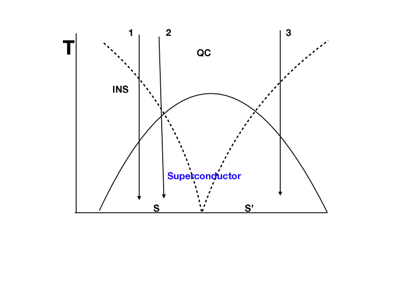
Figure 1: A rough sketch of dimensional crossover of $\rho_{c}$ as a function of temperature $T$. the dashed lines schematically represents quantum critical fans ant the solid dome is the superconducting dome.

INS stands for insulator and QC for quantum critical. Here S and S’ are two phases, both with superconducting order parameters. For example, S may be $d$-density wave along with superconductivity and S’ without the $d$-density wave. Thus there can be a continuous phase transition. Three vertical arrows are possible experimental trajectories that intersect with quantum critical fan describing a crossover scale. These trajectories cross over to the superconducting state. There is no reason for the quantum critical point to be in the middle of the superconducting dome as drawn here for simplicity. The line 2 will have very little insulating up turn.

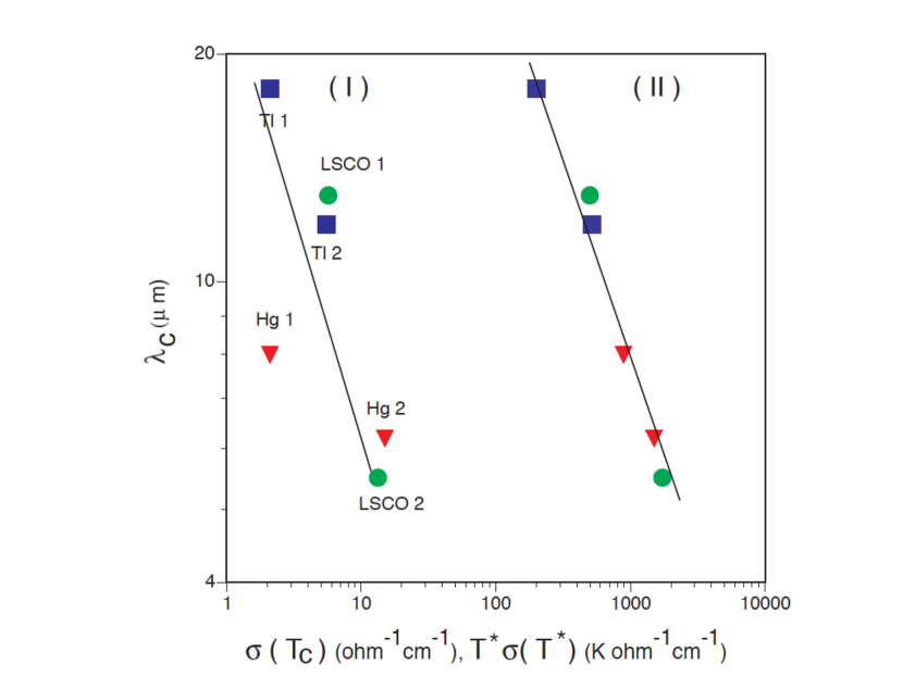
Figure 2: The Basov plot: $\ln\lambda_{c}$ is plotted against $\ln\sigma_{c}(T_{c})$, as in the original Basov plot (I), and against $\ln[T^{*}\sigma_{c}(T^{*})]$ as discussed here (II). The legends in group (II) are the same as those in group (I). Tl1: Ref. [17] Tl2: Ref. [18]; Hg1: Ref. [19], Hg2: Ref. [18]; LSCO 1 (12%), LSCO 2 (15%): Refs. [20, 21, 22]. More recent compilation of data [2] does not change any conclusions.

The expression in Eq. 20 is very interesting. It is cast in the form discussed by Zaanen [1] and shows the importance of Planckian time $\hbar/k_{B}T^{*}$, once again by matching the dimensions. There are two important points worth noting. First $T^{*}$ is not the same as $T_{c}$, the transition temperature; it is merely a characteristic temperature. Second, provided the expression in curly brackets is a universal constant, a plot of $\ln\lambda_{c}$ against $\ln[\sigma_{c}(T^{*})T^{*}]$ should be a universal straight line, independent of material, and temperature $T^{*}$, which is indeed the case, thus validating Eq. (20). Basov et al.[23] suggested a similar correlation by plotting $\ln\lambda_{c}$ against $\ln\sigma_{c}(T_{c})$, shown as (I) in Fig. 2. In comparison to Basov correlation, the correlation discussed here, shown as (II), is excellent. In Fig. 2, we have taken $T^{*}\approx T_{c}$ for those doped materials that show simply a flattening of $\rho_{c}(T)$ close to $T_{c}$; see the discussion above in reference to Fig. 1.

V Discussion

Recall that in order to discuss Planckian dissipation above we had to introduce a sum rule due to Kubo. This sum rule applies independently for any direction. The $c$-axis sum rule has not been discussed in this context to my knowledge. It is notable that I could combine a simple perturbative expansion, thanks to the assumption of lack of quasiparticle pole, with some “empirical” results concerning the $c$-axis resistivity, which is physically clearly justified in Fig. 1. I could have used the $ab$-plane sum rule but in that case a perturbative analysis would not have been applicable because of strong interactions. Later I relied on quantum criticality to arrive at the dissipation scale. Is there any interpretation that we can give to the $T=0$ problem above? A rigorous answer does not exist. I finish by emphasizing that the existence of quantum criticality does not always lead to time scales relevant for dissipation, as discussed in regard to compactification scale [24]. Perhaps one can extend much of the theory to the criticality in the overdoped regime of cuprates [25, 3], recently discussed in Refs.  [26] and [27].

A number of issues are not addressed: I only considered single layer cuprates and said nothing about the multilayer cuprates. Moreover the treatment in the $c$-axis tunneling in a non-Fermi liquid has been heuristic. These difficult questions must be answered in the future.

This work was performed at the Aspen Center for Physics, which is supported by National Science Foundation grant PHY-1607611. It was also partially supported by funds from David S. Saxon Presidential Term Chair at the University of California Los Angeles. I thank Steve Kivelson for a crtical reading of the manuscript.

References

- Zaanen [2004] J. Zaanen, Why the temperature is high, Nature 430, 512 (2004).
- Homes et al. [2004] C. C. Homes, S. V. Dordevic, M. Strongin, D. A. Bonn, R. Liang, W. N. Hardy, S. Komiya, Y. Ando, G. Yu, N. Kaneko, X. Zhao, M. Greven, D. N. Basov, and T. Timusk, A universal scaling relation in high-temperature superconductors, Nature 430, 539 (2004).
- Legros et al. [2019] A. Legros, S. Benhabib, W. Tabis, F. Laliberté, M. Dion, M. Lizaire, B. Vignolle, D. Vignolles, H. Raffy, Z. Z. Li, P. Auban-Senzier, N. Doiron-Leyraud, P. Fournier, D. Colson, L. Taillefer, and C. Proust, Universal -linear resistivity and planckian dissipation in overdoped cuprates, Nature Physics 15, 142 (2019).
- Zaanen [2019] J. Zaanen, Planckian dissipation, minimal viscosity and the transport in cuprate strange metals, SciPost Phys. 6, 61 (2019).
- Hartnoll and Mackenzie [2022] S. A. Hartnoll and A. P. Mackenzie, Colloquium: Planckian dissipation in metals, Rev. Mod. Phys. 94, 041002 (2022).
- Ambegaokar and Baratoff [1963] V. Ambegaokar and A. Baratoff, Tunneling between superconductors, Phys. Rev. Lett. 10, 486 (1963).
- Chakravarty and Anderson [1994] S. Chakravarty and P. W. Anderson, Interlayer Josephson tunneling and breakdown of fermi liquid theory, Phys. Rev. Lett. 72, 3859 (1994).
- Boebinger et al. [1996] G. S. Boebinger, Y. Ando, A. Passner, T. Kimura, M. Okuya, J. Shimoyama, K. Kishio, K. Tamasaku, N. Ichikawa, and S. Uchida, Insulator-to-metal crossover in the normal state of near optimum doping, Phys. Rev. Lett. 77, 5417 (1996).
- Chakravarty et al. [1988] S. Chakravarty, B. I. Halperin, and D. R. Nelson, Low-temperature behavior of two-dimensional quantum antiferromagnets, Phys. Rev. Lett. 60, 1057 (1988).
- Chakravarty et al. [1989] S. Chakravarty, B. I. Halperin, and D. R. Nelson, Two-dimensional quantum heisenberg antiferromagnet at low temperatures, Phys. Rev. B 39, 2344 (1989).
- Shastry and Sutherland [1990] B. S. Shastry and B. Sutherland, Twisted boundary conditions and effective mass in Heisenberg-ising and Hubbard rings, Phys. Rev. Lett. 65, 243 (1990).
- Kubo [1957] R. Kubo, Statistical-mechanical theory of irreversible processes. i. general theory and simple applications to magnetic and conduction problems, Journal of the Physical Society of Japan 12, 570 (1957).
- Tinkham [1996] M. Tinkham, Introduction to Superconductivity (Mc-Graw-Hill, 1996).
- Ando et al. [1995] Y. Ando, G. S. Boebinger, A. Passner, T. Kimura, and K. Kishio, Logarithmic divergence of both in-plane and out-of-plane normal-state resistivities of superconducting in the zero-temperature limit, Phys. Rev. Lett. 75, 4662 (1995).
- Yin and Chakravarty [1998] L. Yin and S. Chakravarty, Spectral anomaly and high temperature superconductors, Int. J. Mod. Phys. B 58, R559 (1998).
- Doiron-Leyraud et al. [2007] N. Doiron-Leyraud, C. Proust, D. LeBoeuf, J. Levallois, J.-B. Bonnemaison, R. Liang, D. A. Bonn, W. N. Hardy, and L. Taillefer, Quantum oscillations and the fermi surface in an underdoped high-tc superconductor, Nature 447, 565 (2007).
- Moler et al. [1998] K. A. Moler, J. R. Kirtley, D. G. Hinks, T. W. Li, and M. Xu, Images of interlayer josephson vortices in , Science 279, 1193 (1998).
- Basov et al. [1999] D. N. Basov, S. I. Woods, A. S. Katz, E. J. Singley, R. C. Dynes, M. Xu, D. G. Hinks, C. C. Homes, and M. Strongin, Sum rules and interlayer conductivity of high-tc cuprates, Science 283, 49 (1999).
- Kirtley et al. [1998] J. R. Kirtley, K. A. Moler, G. Villard, and A. Maignan, -axis penetration depth of hg-1201 single crystals, Phys. Rev. Lett. 81, 2140 (1998).
- Loram et al. [1994] J. Loram, K. Mirza, J. Wade, J. Cooper, and W. Liang, The electronic specific heat of cuprate superconductors, Physica C: Superconductivity 235-240, 134 (1994).
- Uchida et al. [1996] S. Uchida, K. Tamasaku, and S. Tajima, -axis optical spectra and charge dynamics in , Phys. Rev. B 53, 14558 (1996).
- Nakamura and Uchida [1993] Y. Nakamura and S. Uchida, Anisotropic transport properties of single-crystal : Evidence for the dimensional crossover, Phys. Rev. B 47, 8369 (1993).
- Basov et al. [1994] D. N. Basov, T. Timusk, B. Dabrowski, and J. D. Jorgensen, c-axis response of : A pseudogap and possibility of josephson coupling of planes, Phys. Rev. B 50, 3511 (1994).
- Chakravarty [1996] S. Chakravarty, Dimensional crossover in quantum antiferromagnets, Phys. Rev. Lett. 77, 4446 (1996).
- Kopp et al. [2007] A. Kopp, A. Ghosal, and S. Chakravarty, Competing ferromagnetism in high temperature copper oxide superconductors, Proc. National Acad. Sciences, USA 104, 6123 (2007).
- Koshi et al. [2018] K. Koshi, A. Tadashi, M. S. Kensuke, F. Yasushi, K. Takayuki, N. Takashi, M. Hitoshi, Isao.W., M. Masanori, K. Akihiro, K. Ryosuke, and Y. Koike, Development of ferromagnetic fluctuations in heavily overdoped copper oxides, Phys. Rev. Lett, 121, 057002 (2018).
- Sarkar et al. [2020] T. Sarkar, D. S. Wei, J. Zhang, N. R. Poniatowski, P. R. Mandal, A. Kapitulnik, and R. L. Greene, Competing ferromagnetism in high temperature copper oxide superconductors in heavily overduped, Science 368, 532 (2020).