Logarithmic Regret for Matrix Games against an Adversary with Noisy Bandit Feedback
Abstract
This paper considers a variant of zero-sum matrix games where at each timestep the row player chooses row , the column player chooses column , and the row player receives a noisy reward with mean . The objective of the row player is to accumulate as much reward as possible, even against an adversarial column player. If the row player uses the EXP3 strategy, an algorithm known for obtaining regret against an arbitrary sequence of rewards, it is immediate that the row player also achieves regret relative to the Nash equilibrium in this game setting. However, partly motivated by the fact that the EXP3 strategy is myopic to the structure of the game, O’Donoghue et al. (2021) proposed a UCB-style algorithm that leverages the game structure and demonstrated that this algorithm greatly outperforms EXP3 empirically. While they showed that this UCB-style algorithm achieved regret, in this paper we ask if there exists an algorithm that provably achieves regret against any adversary, analogous to results from stochastic bandits. We propose a novel algorithm that answers this question in the affirmative for the simple setting, providing the first instance-dependent guarantees for games in the regret setting. Our algorithm overcomes two major hurdles: 1) obtaining logarithmic regret even though the Nash equilibrium is estimable only at a rate, and 2) designing row-player strategies that guarantee that either the adversary provides information about the Nash equilibrium, or the row player incurs negative regret. Moreover, in the full information case we address the general case where the first hurdle is still relevant. Finally, we show that EXP3 and the UCB-based algorithm necessarily cannot perform better than .
1 Introduction
This paper considers a two-player zero-sum repeated game where the environment, or game matrix, is unknown before the start of play. At the beginning of each round each player simultaneously chooses amongst a finite set of actions, and then observes their respective rewards which are equal and opposite (hence, zero-sum), and stochastic. For example, consider two firms in a duopoly competing for customers. On any given week, prospective clients submit bids to both firms, and the first firm may offer lower prices whereas the second firm may offer a more valuable warranty. At the end of the week, both firms know which actions each other took, and what share of the customers or revenue they received. This game is challenging for two reasons: first, neither firm knows precisely what outcome will occur for any given pair of actions due to uncertainty and stochasticity in the market, and second, they are competing against each other where one firm’s gain is the other firm’s loss.
When interacting in a stochastic environment, each player is motivated to explore the environment to identify high-reward actions that can be exploited against their opponent. However, unlike a multi-armed bandit game where agents can control how they explore, in this competitive game an opponent can actually prevent the agent from observing part of the game matrix by simply refusing to play some actions. For example, in a game of rock-paper-scissors, if the second player never plays “rock” the first player never learns how their actions compete with “rock” unless they assumed the game was symmetric. However, in this case the first player can play a randomized strategy of over (“rock”,“scissors”) to get an higher expected reward than it gets by playing the equilibrium strategy over (“rock”,“paper”,“scissors”).
This paper formally studies situations like those illustrated above in a problem setting at the intersection of multi-armed bandits and game theory. Specifically, we are interested in the limits of an agent acting in a stochastic environment against an adversarial opponent trying to obtain as much reward as possible. Similar questions have been posed before and so-called “no-regret” algorithms have played a vital role in understanding game dynamics and computing various equilibrium concepts in multi-player games (Daskalakis et al., 2011; Chen and Peng, 2020; Cai and Daskalakis, 2011; Freund and Schapire, 1999; Rakhlin and Sridharan, 2013; Syrgkanis et al., 2015; Wei et al., 2021). A key feature of these algorithms in the repeated-play setting is that the players adapt based on the feedback they receive. This paper diverges from this work by assuming that the game matrix is unknown and only noisy observations of its entries are available. Outside of game theory, multi-armed bandits for regret minimization has been widely studied in scenarios where we observe noisy samples of the input (Auer et al., 2002a; Agrawal and Goyal, 2017; Kaufmann et al., 2012, 2016). This paper works at the intersection of the repeated-play setting and the noisy observation setting in order to focus on a regret minimization problem in a two-player zero-sum matrix game where players observe the element of the matrix with some sub-Gaussian noise when they query it. Our work is inspired by the a recent work of O’Donoghue et al. (2021) that introduced this setting.
1.1 Problem Setting
Let us first establish some notion for zero-sum matrix games. Consider a matrix . Let denote the -dimensional simplex, and let denote the usual canonical vector whose -th coordinate is one and rest of the coordinates are zero. A pair of strategies is a Nash equilirium if the following inequalities hold:
In this paper, we will assume the Nash equilibrium is unique, a common assumption in the literature (Daskalakis and Panageas, 2019; Wei et al., 2021; Bailey and Piliouras, 2018) as the set of matrices with non-unique Nash equilibrium is closed and has a Lebesgue measure of zero in the space of all matrices (Van Damme, 1991). In this case, we have where . Let
denote the value of matrix game on , where the exchange of the min and max is guaranteed by Von Neumann’s minimax theorem (v. Neumann, 1928).
For any fixed with a unique Nash equilibrium , consider the following two-player repeated-game: in each round , the row player chooses a strategy against an adversarial column player that chooses a strategy . Then, a random matrix is drawn IID where . Next, a row index is sampled from the distribution , and a column index is sampled from the distribution . At the end of round , the row player observes the column index and receives one of the following forms of feedback:
-
•
Full feedback setting: The row player observes .
-
•
Bandit feedback setting: The row player observes only the entry of corresponding to row and column indices played: .
We are interested in only controlling the row-player and aim to maximize its expected cumulative reward while playing against a potentially adversarial column-player. Before the start of the game, the matrix is unknown to the row-player. We make no assumptions about the adversarial column-player, and even allow them to have knowledge of and the matrix . After time periods, we consider two measures of performance for the row-player:
and another quantity defined with respect to a mixed strategy Nash equilibrium :
By adding and subtracting in each term of and applying the properties of Nash equilibria, it follows that . Moreover, it is known that there exists a row-player strategy (e.g., EXP3) such that against any column-player adversary. However, we argue next that external regret does not adequately capture incentives of the two players.
Claim 1 (Informal, see Appendix B.3).
Fix to encode rock-paper-scissors so that . For any row-player that enjoys against any adversary, there exists an adversarial column-player such that and , where are absolute constants.
On the one hand, given that EXP3 achieves on this instance, the adversary of the claim appears to be applying maximum pain to the row-player. On the other hand, we observe that the column-player is suffering linear Nash regret. This is the equivalent of two firms competing for market share in a game where, if playing optimally at the Nash equilibrium, both players would split the market 50/50. But instead, the column-player that aims to maximize the external regret of the row-player is ceding market share and splitting the market 75/25 in the row-player’s favor! This example shows that for two strategic agents that are self-interested, Nash regret is a far more representative notion of regret.
Besides our above argument for studying Nash regret, to our knowledge O’Donoghue et al. (2021) was the first work to consider our precise setting, and they also adopted Nash regret as the metric of interest. Though EXP3 is known to obtain a external regret (which implies a Nash regret of the same order), O’Donoghue et al. (2021) designed an Upper Confidence Bound (UCB) algorithm motivated by the observation that empirically, UCB seems to perform much better than EXP3. UCB’s superior empirical performance was conjectured to be attributed to the algorithm’s exploitation of the game structure that EXP3 ignores, even though no theoretical advantage could be shown. This observation leads us to ask the following question:
Do there exist conditions under which an algorithm can achieve poly-logarithmic Nash regret against an adversary with respect to the time horizon ?
We answer this question in the affirmative for matrices in the full-information case, and matrices in the bandit feedback case. In the sections that follow, we state our main results, describe the major pieces of the algorithms and analysis, and then finish by placing our results in the context of prior work.
2 Logarithmic regret with bandit feedback main result
We begin with our main result on instance-dependent poly-logarithmic regret for matrix games with bandit feedback in the case. When we move to full feedback, we will address the more general case. The case is enough to communicate the challenges and novelty of our solution for the bandit case.
Theorem 1.
Fix a game matrix with a unique Nash equilibrium. There exists an algorithm (see Appendix F) that incurs a Nash regret of at most where and are absolute constants and .
Before describing the algorithm and its analysis, we take a moment to see why other common algorithms fail to achieve this result and justify our setting’s assumptions.
2.1 The failure of myopic multi-armed bandit algorithms
Consider playing a multi-armed bandit algorithm over the arms (actions in the game) as the row-player for rounds, such as EXP3 or any other mirror descent algorithm. For the matrix
if the column-player plays for all rounds, then from the perspective of the multi-armed bandit algorithm, this is just a two-armed stochastic multi-armed bandit instance with Bernoulli arms having means . In this case the algorithm will pull each arm an equal number of times in expectation. However, if the column-player alternatively played and the bandit algorithm continued to play both arms equally in expectation, then the bandit algorithm would receive total expected reward, translating to a Nash regret of since the value of the game . Since rounds are not sufficient to discriminate between and , we can argue that any bandit algorithm will incur Nash regret in expectation. However, for this same matrix, our theorem evaluates to Nash regret. We refer the reader to Appendix B.4 for a formal proof that leads to this intuition.
2.2 The failure of the matrix-game UCB algorithm of O’Donoghue et al. (2021)
One of our primary motivations for this work was the observation in (O’Donoghue et al., 2021) that their proposed matrix-game UCB algorithm which takes advantage of the matrix structure of the game appeared to significantly outperform EXP3 empirically. While the last subsection implies EXP3 cannot hope to do better than Nash regret, perhaps this matrix-game UCB algorithm achieves Nash regret. To our surprise, we showed it cannot. Consider the matrix . Observe that has a unique Nash equilibrium . We claim that UCB incurs a regret on the matrix game even in the non-stochastic setting. We first provide a high-level description of how the column-player chooses in each round . There are two key phases: (1) burn-in phase and (2) best-response phase. In the burn-in phase, the column-player chooses strategies that are close to in order to force UCB to explore all the elements of sufficiently. This phase lasts for roughly rounds. Next, in the best response phase, the column players chooses the best response .
We now provide an intuition behind the regret incurred by UCB. Let for all . Suppose the burn-in phase ends at time step (which is roughly ). At the end of the burn-in phase, we have . UCB maintains an upper confidence matrix
and plays in each round. In the best response phase, if for rounds (where is some constant) we have , then the regret incurred by the row-player during these rounds is at least .
Let us now argue that this condition holds. First, at the time step (i.e., the end of the burn-in phase), we have
Now, observe that . This implies that for , we have that . Hence, starting from where , it takes (where is a constant) steps for to become . Hence, UCB incurs a regret of . However, for this matrix, our main theorem evaluates to Nash regret.
At a very high-level, UCB may be reacting too slowly by moving only each round. As we will see in a moment, our algorithm moves about per round. We refer the reader to Appendix B.5 for a more formal analysis.
2.3 Variations on assumptions
Actions observed.
In the bandit feedback setting, we have that the row-player observes both the random reward associated with the two players’ actions , and the action that the column-player played. Theorem 1 claims that there is an algorithm that achieves logarithmic regret. Observing the column-player’s action is not always available in all settings. For example, in a duopoly of ride-sharing firms we may observe the outcome of a competitor’s actions, but we do not know precisely which actions they took to match riders with drivers on any particular day. Sadly, we show that observing the opponent’s action is necessary for obtaining logarithmic regret, even in the full-information setting where there is no issue of exploration. Fix
| (1) |
where , and , and consider the following theorem, the proof of which is provided in Appendix B.1.
Theorem 2.
With and defined in (1), let an instance be fixed before play starts. At each time , the row- and column-players choose and , respectively, actions and are drawn, and the row-player receives reward and observes where . If an algorithm constructs from alone (and not ) then the best response strategy satisfies
where .
While the best-response strategy of the column-player may appear like a strong adversary, such an assumption is standard and even natural if one assumes the adversary knows the row-player’s algorithm (but not their source of randomness for which ).
Nash versus external regret.
Our result is proven with respect to Nash regret. When introducing this notion, we pointed out that external regret is an upper bound on Nash regret for any game. Given that it is possible to obtain logarithmic Nash regret, is it also possible to obtain logarithmic external regret? Our next theorem rules this out.
Theorem 3.
Consider a matrix with a unique full support Nash Equilibrium. For any algorithm, there exists an adversary that plays in each round such that
where is an absolute constant.
Interestingly, the above theorem is in the non-stochastic setting meaning that the row-player has knowledge of exactly and can use it to choose its actions. This is because in the proof (see Appendix B.2), the external regret comes from the unpredictability of the opponent, not the game matrix. Nevertheless, for the same matrix our algorithm achieves logarithmic nash regret against any adversary.
3 Algorithms for logarithmic regret in games
The algorithm that achieves the main result (Theorem 1), to be frank, is not easy to describe or understand at first. In the same way that EXP3 and its analysis is easier to understand after first understanding multiplicative weights, we will first explain our algorithm with full-information feedback, and then describe how we generalize to the bandit case. However, we point out that at a high-level, the full-information and bandit feedback algorithms have many common characteristics. Both algorithms begin with a burn-in phase of exploration that lasts until statistics about concentrate. This burn-in phase can incur substantial regret if continued indefinitely, but since its length depends on problem-dependent constants it contributes at most to the overall regret.
Once this burn-in phase terminates after roughly rounds, the algorithms then allocates samples to a sub-routine which incurs regret. When the sub-routine returns, we then update statistics and execute the subroutine with samples. Since each execution of the sub-routine incurs regret, and it can only be executed at most times due to its exponentially growing time-scale, we conclude with a regret bound. Most of the interesting bits of the algorithm occur in the sub-routine, so we begin there. The main difference between the full-information and bandit case is the initial exploration phase. While in the former case we observe every entry of the matrix at each time, in the bandit case the adversary could prevent us from viewing parts of the matrix which slows our progress in estimating necessary statistics to run the sub-routine. However, if the adversary is withholding information in this way, this necessarily means we are receiving negative regret. The next few sections shed a bit more light on the procedures.
3.1 Subroutine for matrix games with full support (full or bandit feedback)
Assume the algorithm has just completed the burn-in phase and calls the sub-routine for the first time. As input, the sub-routine is given an empirical matrix where it is guaranteed that its expectation has a full-support Nash equilibrium, established in the burn-in phase. The sub-routine is also given where is the Nash equilibrium of , a parameter we will describe later, and time-period to run for (in the bandit case, describes the the number of times every entry of the matrix must be observed before terminating). Assume that
| (2) |
where is the unique full-support Nash equilibrium of the matrix .
The psuedo-code for the sub-routine is given in Algorithm 1. At a high-level, the algorithm is acting like any online-learner like exponential weights (Slivkins et al., 2019) acting on a series of reward vectors with . The fact that our algorithm acts on instead of only is just to ensure that remains in the simplex since we only explicitly update its first components. At each time the algorithm plays where for all and . Notice that the statistics of remain constant throughout an execution of the subroutine. These last two facts will be critical in our analysis. The sub-routine enjoys the following guarantee.
Theorem 4.
Proof sketch..
Through a series of algebraic manipulations we show that
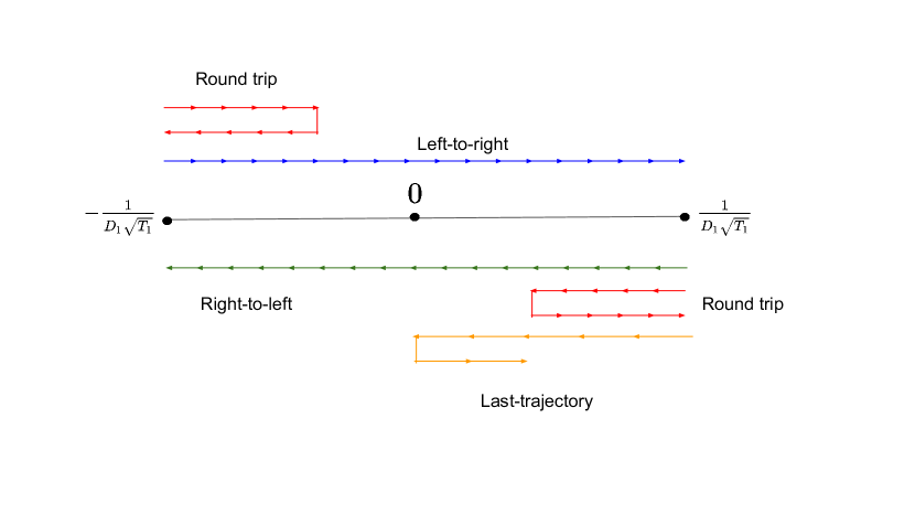
where . If we partition the trajectory into such that within an interval we have so that no projection is necessary, then on this interval we can derive a closed-form expression for . It turns out this sum can be quite large in magnitude. But by exploiting the closed-form expression we can show that this sum can be both very positive and very negative, and these large magnitude pieces cancel out. To do this we classify each interval into one of a few cases.
In the first case, a round-trip occurs such that . In this case the large positive and negative terms of the sum start cancelling out each other and at the end the sum will scale like . In the second case, the trajectory of starts from the left-most point of the interval and travels to the right-most point of this interval. The third case is the opposite direction. Again, the sum of each interval is not small in magnitude, but by pairing one left-to-right trajectory with one right-to-left trajectory, we can simulate a round trip. Similar to the first case, the large negative terms of the sum from one of the trajectory starts cancelling out the large positive terms of the sum from the other trajectory and hence the combined sum of both trajectory will scale like . The final case that ends in the middle at time contributes just constant regret. We conclude that
∎
The full proof of Theorem 4 is found in Appendix C.1. The same intuition behind this proof and result also hold for the bandit case. Mechanically, the only difference is that instead of specifying how many iterations to run the sub-routine for, namely , the sub-routine is still given as input, but told to terminate only after every entry of the matrix has been observed at least times. Consequently, in the analysis found in Appendix C.2 of the bandit case we have to bound the regret by considering two cases: either the time to achieve this minimum sampling number is small, or we receive negative regret. Either way the total regret is bounded.
3.2 Algorithm for Full-information feedback
If is the unique Nash eqiulibrium of , then the analysis follows three major steps: (1) identify the sub-matrix of associated with the support of , then (2) confirm that statistics have been estimated accurately enough to start calling out to the sub-routine, and finally (3) play the sub-routine repeatedly until the final time horizon is reached.
Identifying the sub-matrix.
During this phase we play the Nash equilibrium of the running empirical average matrix . This phase lasts at most steps, scaled by some problem-dependent constants. Assume so there is something to do in this step, and define , , and . To identify the support, we use empirical plug-in estimates to estimate the Nash equilbrium and compute the gaps. Eventually, we sample enough to rule out indices with positive gap and confirm those indices in the support by verifying that the coefficients are positive using confidence intervals.
Confirm concentration of matrix estimates.
Assume we have identified the optimal sub-matrix of associated with the support of the Nash equilibrium. To simplify notation, rename this sub-matrix and assume is . If is the unique Nash eqiulibrium of then . Similarly, which implies . Since sums to we conclude that and . Define
If then there exists an that depends only on such that . So if we set then
if . If then clearly . Thus, we have that the above inequality is valid as soon as . At this point, we can start invoking the sub-routine with , , , and .
Final regret bound.
After repeatedly playing the sub-routine and setting and after each invocation, we can obtain the following final regret bound.
Theorem 5.
Fix a matrix game on with a unique Nash equilibrium of support size . Let be defined with respect to the sub-matrix of associated the support of . Then
where depend only on .
3.3 Algorithm for Bandit feedback
We now focus on games under bandit feedback. Unlike the full feedback case, we are not guaranteed that every element would be explored equally. Hence, in each round , we have to play a strategy such that either every element would be explored sufficiently or we incur a negative regret. We achieve this goal by designing a complicated exploration procedure. Here we describe the key parts of the exploration procedure.
Consider a matrix . Our aim is to estimate the gaps up to a constant factor. We begin with an uniform exploration phase where we aim to estimate two such gaps up to a constant factor. First, we play in each round. We eventually estimate one of the gaps up to a constant factor due to the fact that one of the columns must be played at least half the time. Then, we play one of the two strategies and ( depends on the gap that we have estimated previously up to a constant factor) in each round. We eventually estimate one more gap up to a constant factor (again due to the fact that one of the columns must be played at least half the time).
Let us assume that we have estimated the gaps and up to a constant factor by the end of the uniform exploration phase. Now we aim to estimate the gap up to a constant factor. We do this by playing a strategy that incurs a non-positive regret if column one is played by the column-player. In turn, the column-player is forced to play the second column if it wants the row-player to incur positive regret. Hence, we end up estimating the gap up to a constant factor. Now, we aim to estimate the final gap up to a constant factor. We do this by finding a strategy that incurs a non-positive regret if column two is played by the column-player. Hence if the row-player plays the column-player is forced to play the first column if it wants the row-player to incur positive regret.
Using the strategies and we estimate the final gap as follows. We play until the column two is played by the column player. We then switch to and play it until column one is played by the column-player. We then switch back to and repeat this process until we estimate the gap up to a constant factor. This concludes our exploration procedure.
After this initial exploration phase is over, if we observe that the matrix game on has a pure strategy Nash equilibrium , then we play for the rest of the rounds. Otherwise, we invoke the sub-routine similarly to the full-information case. Putting it all together, we obtain our main result of Theorem 1 for bandit feedback. The complete algorithm for bandit feedback and the full proof of Theorem 1 is in Appendix F.
4 Experiments
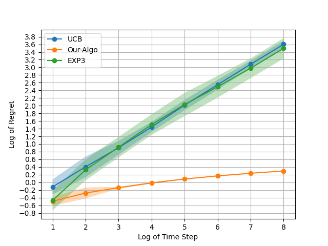
In this section, we compare the empirical performance of our algorithm for bandit feedback111We make a small modification in our algorithm by executing the sub-routine in Algorithm 1 right from the start. against the UCB algorithm from O’Donoghue et al. (2021) and Exp3 from Auer et al. (2002b). We consider the input matrix and three different adversaries for the experiments. For each adversary, we run the three algorithms for eight different time horizons ( and plot the logarithm of total Nash Regret incurred against the logarithm of each time horizon (also referred to as the log-log plot). Code to replicate these experiments is available at https://github.com/AistatsRegret24/code.
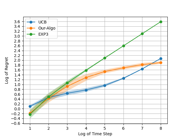
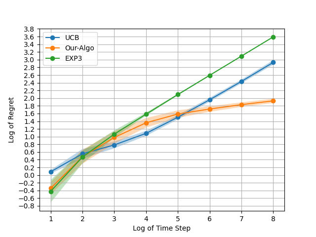
First in figure 1(a), we consider an adversary that for a given horizon plays the equilibrium strategy for the first steps and plays the best-response strategy for the next steps. Next in figure 1(b), we consider an adversary that plays only the best-response strategy for all the steps. Finally in figure 1(c), we consider an adversary that for a given horizon plays either the equilibrium strategy or the best-response strategy depending on the strategy played by the algorithm for the first steps and plays the best-response strategy for the next steps.
In all three log-log plots we observe that our algorithm performs better than UCB and EXP3 as the time horizon grows. Moreover, in all three log-log plots we observe that our algorithm has a decreasing slope suggesting sub-polynomial regret consistent with polylog(), whereas the slopes of UCB and EXP3 approach , suggesting a regret.
5 Related Work
Multi-Armed Bandits. Instance-dependent regret bounds for the problem of regret minimization has been studied extensively in the context of stochastic multi-armed bandits. Auer et al. (2002a) showed an instance-dependent upper bound of for the Upper confidence bound algorithm where is the difference between the means of the best-arm and the optimal arm. Agrawal and Goyal (2017) and Kaufmann et al. (2012) subsequently showed a similar instance-dependent upper bound for the Thompson sampling. Instance dependent sample complexity bounds has also been widely studied in multi-armed bandits. Jamieson et al. (2014) showed an instance-dependent upper bound of for the best-arm identification problem. Kaufmann et al. (2016) showed instance-dependent lower bounds for the best-arm identification problem.
Learning in Games. O’Donoghue et al. (2021) first studied the matrix games under the bandit feedback setting and provided a cumulative regret upper bound for the UCB algorithm. They also provided a Bayesian regret upper bound for the K-learning algorithm. Cui et al. (2022) also studied a related regret minimization problem for congestion games under bandit feedback setting. There has also been work on analyzing Nash regret in time-varying zero-sum matrix games (Cardoso et al., 2019; Zhang et al., 2022). Recently, Maiti et al. (2023) initiated a study on instance-dependent sample complexity bounds for computing approximate equilibrium concepts in two-player zero-sum matrix games.
No-regret learning has also been an area of significant interest in the non-stochastic setting as the average-iterate dynamics converge to a Nash equilibrium. Worst-case external regret bound in repeated play setting is known to be (Cesa-Bianchi and Lugosi, 2006). However, when the players are not adversarial and instead are competing with each other, there exists strongly uncoupled dynamics that converge at a rate in two-player zero-sum matrix games (Daskalakis et al., 2011). Daskalakis et al. (2011) also achieved a Nash regret of when both the players play the same algorithm. Rakhlin and Sridharan (2013) also showed a convergence rate to a Nash Equilibrium for a version of Optimistic mirror descent. Kangarshahi et al. (2018) later designed a no-regret algorithm based on Optimistic mirror descent that achieved a convergence rate with respect to the value of game.
Recently, the last-iterate guarantees of no-regret algorithms have also been studied (Daskalakis et al., 2018; Mokhtari et al., 2020; Mertikopoulos et al., 2019; Daskalakis and Panageas, 2019; Lei et al., 2021; Cen et al., 2021). Gradient descent ascent and multiplicative weights update either diverge away from the equilibrium or cycle around the equilibrium even in simple instances (Mertikopoulos et al., 2018; Bailey and Piliouras, 2018). Wei et al. (2021) showed that the optimistic versions of these no-regret algorithms exhibit linear last-iterate convergence in two-player zero-sum matrix games. Abe et al. (2023) also showed a similar last-iterate convergence result in noisy-feedback setting.
The no-regret learning framework has also been studied in the multi-player game setting (Syrgkanis et al., 2015; Chen and Peng, 2020; Blum and Mansour, 2007; Hart and Mas-Colell, 2000; Foster and Vohra, 1997). Daskalakis et al. (2021) showed that a variant of multiplicative weight update achieves an external regret of in multi-player general sum games. Anagnostides et al. (2022a) later extended this result to swap regret. Recently, Anagnostides et al. (2022b) designed an uncoupled dynamics that has a swap regret of in general-sum multi-player games.
6 Conclusion
This paper presents a study of a regret minimization problem in matrix games that was first analyzed by O’Donoghue et al. (2021). In the full-feedback setting, we provide instance-dependent poly-logarithmic regret for any matrix game. In the bandit-feedback setting, we provide instance-dependent poly-logarithmic regret for any matrix game. To the best of our knowledge, these are the first instance-dependent guarantees in these settings. However, several questions remain unresolved. One natural direction is to establish instance-dependent lower bounds in the full-feedback setting. The main challenge is to design hard alternative instances to the input matrix, and characterize the adversarial behavior of the column-player. Another important direction is to improve our upper bounds in the full-feedback setting, especially with respect to the input dimensions and . Our algorithms estimate the determinant of certain matrices up to a constant factor, which leads to non-optimal bounds on and . To achieve optimal bounds, we need to devise methods that do not heavily rely on the Nash Equilibrium of the empirical matrix. The existence of instance-dependent poly-logarithmic regret for arbitrary matrix games in the bandit feedback setting also remains an unanswered question, and the major challenge is to sufficiently explore all the elements while incurring low regret.
In addition to zero-sum matrix games, various important problems such as general sum games and zero-sum Markov games can be studied in the noisy setting , and instance-dependent bounds can be developed for appropriate regret minimization problems from the perspective of a single player. Moreover, one might extend our problem setting to cooperative games where players form a coalition to achieve a desirable outcome.
ACKNOWLEDGEMENTS
The first author thanks Claire Zhang for the useful discussions. This work was supported in part by NSF awards RI 1907907 and TRIPODS 2023166.
References
- Abe et al. (2023) Kenshi Abe, Kaito Ariu, Mitsuki Sakamoto, Kentaro Toyoshima, and Atsushi Iwasaki. Last-iterate convergence with full and noisy feedback in two-player zero-sum games. In International Conference on Artificial Intelligence and Statistics, pages 7999–8028. PMLR, 2023.
- Agrawal and Goyal (2017) Shipra Agrawal and Navin Goyal. Near-optimal regret bounds for thompson sampling. Journal of the ACM (JACM), 64(5):1–24, 2017.
- Anagnostides et al. (2022a) Ioannis Anagnostides, Constantinos Daskalakis, Gabriele Farina, Maxwell Fishelson, Noah Golowich, and Tuomas Sandholm. Near-optimal no-regret learning for correlated equilibria in multi-player general-sum games. In Proceedings of the 54th Annual ACM SIGACT Symposium on Theory of Computing, pages 736–749, 2022a.
- Anagnostides et al. (2022b) Ioannis Anagnostides, Gabriele Farina, Christian Kroer, Chung-Wei Lee, Haipeng Luo, and Tuomas Sandholm. Uncoupled learning dynamics with swap regret in multiplayer games. In Advances in Neural Information Processing Systems, 2022b.
- Auer et al. (2002a) Peter Auer, Nicolo Cesa-Bianchi, and Paul Fischer. Finite-time analysis of the multiarmed bandit problem. Machine learning, 47:235–256, 2002a.
- Auer et al. (2002b) Peter Auer, Nicolo Cesa-Bianchi, Yoav Freund, and Robert E Schapire. The nonstochastic multiarmed bandit problem. SIAM journal on computing, 32(1):48–77, 2002b.
- Bailey and Piliouras (2018) James P Bailey and Georgios Piliouras. Multiplicative weights update in zero-sum games. In Proceedings of the 2018 ACM Conference on Economics and Computation, pages 321–338, 2018.
- Blum and Mansour (2007) Avrim Blum and Yishay Mansour. From external to internal regret. Journal of Machine Learning Research, 8(6), 2007.
- Bohnenblust et al. (1950) HF Bohnenblust, S Karlin, and LS Shapley. Solutions of discrete, two-person games. Contributions to the Theory of Games, 1:51–72, 1950.
- Cai and Daskalakis (2011) Yang Cai and Constantinos Daskalakis. On minmax theorems for multiplayer games. In Proceedings of the twenty-second annual ACM-SIAM symposium on Discrete algorithms, pages 217–234. SIAM, 2011.
- Cardoso et al. (2019) Adrian Rivera Cardoso, Jacob Abernethy, He Wang, and Huan Xu. Competing against Nash equilibria in adversarially changing zero-sum games. In International Conference on Machine Learning, pages 921–930. PMLR, 2019.
- Cen et al. (2021) Shicong Cen, Yuting Wei, and Yuejie Chi. Fast policy extragradient methods for competitive games with entropy regularization. Advances in Neural Information Processing Systems, 34:27952–27964, 2021.
- Cesa-Bianchi and Lugosi (2006) Nicolo Cesa-Bianchi and Gábor Lugosi. Prediction, learning, and games. Cambridge university press, 2006.
- Chen and Peng (2020) Xi Chen and Binghui Peng. Hedging in games: Faster convergence of external and swap regrets. Advances in Neural Information Processing Systems, 33:18990–18999, 2020.
- Cui et al. (2022) Qiwen Cui, Zhihan Xiong, Maryam Fazel, and Simon Shaolei Du. Learning in congestion games with bandit feedback. In Advances in Neural Information Processing Systems, 2022.
- Daskalakis and Panageas (2019) C Daskalakis and Ioannis Panageas. Last-iterate convergence: Zero-sum games and constrained min-max optimization. In 10th Innovations in Theoretical Computer Science (ITCS) conference, ITCS 2019, 2019.
- Daskalakis et al. (2011) Constantinos Daskalakis, Alan Deckelbaum, and Anthony Kim. Near-optimal no-regret algorithms for zero-sum games. In Proceedings of the twenty-second annual ACM-SIAM symposium on Discrete Algorithms, pages 235–254. SIAM, 2011.
- Daskalakis et al. (2018) Constantinos Daskalakis, Andrew Ilyas, Vasilis Syrgkanis, and Haoyang Zeng. Training gans with optimism. In International Conference on Learning Representations (ICLR 2018), 2018.
- Daskalakis et al. (2021) Constantinos Daskalakis, Maxwell Fishelson, and Noah Golowich. Near-optimal no-regret learning in general games. Advances in Neural Information Processing Systems, 34:27604–27616, 2021.
- Foster and Vohra (1997) Dean P Foster and Rakesh V Vohra. Calibrated learning and correlated equilibrium. Games and Economic Behavior, 21(1-2):40, 1997.
- Freund and Schapire (1999) Yoav Freund and Robert E Schapire. Adaptive game playing using multiplicative weights. Games and Economic Behavior, 29(1-2):79–103, 1999.
- Hart and Mas-Colell (2000) Sergiu Hart and Andreu Mas-Colell. A simple adaptive procedure leading to correlated equilibrium. Econometrica, 68(5):1127–1150, 2000.
- Jamieson et al. (2014) Kevin Jamieson, Matthew Malloy, Robert Nowak, and Sébastien Bubeck. lil’ucb: An optimal exploration algorithm for multi-armed bandits. In Conference on Learning Theory, pages 423–439. PMLR, 2014.
- Kangarshahi et al. (2018) Ehsan Asadi Kangarshahi, Ya-Ping Hsieh, Mehmet Fatih Sahin, and Volkan Cevher. Let’s be honest: An optimal no-regret framework for zero-sum games. In International Conference on Machine Learning, pages 2488–2496. PMLR, 2018.
- Kaufmann et al. (2012) Emilie Kaufmann, Nathaniel Korda, and Rémi Munos. Thompson sampling: An asymptotically optimal finite-time analysis. In Algorithmic Learning Theory: 23rd International Conference, ALT 2012, Lyon, France, October 29-31, 2012. Proceedings 23, pages 199–213. Springer, 2012.
- Kaufmann et al. (2016) Emilie Kaufmann, Olivier Cappé, and Aurélien Garivier. On the complexity of best arm identification in multi-armed bandit models. Journal of Machine Learning Research, 17:1–42, 2016.
- Lei et al. (2021) Qi Lei, Sai Ganesh Nagarajan, Ioannis Panageas, et al. Last iterate convergence in no-regret learning: constrained min-max optimization for convex-concave landscapes. In International Conference on Artificial Intelligence and Statistics, pages 1441–1449. PMLR, 2021.
- Maiti et al. (2023) Arnab Maiti, Kevin Jamieson, and Lillian Ratliff. Instance-dependent sample complexity bounds for zero-sum matrix games. In International Conference on Artificial Intelligence and Statistics, pages 9429–9469. PMLR, 2023.
- Mertikopoulos et al. (2018) Panayotis Mertikopoulos, Christos Papadimitriou, and Georgios Piliouras. Cycles in adversarial regularized learning. In Proceedings of the Twenty-Ninth Annual ACM-SIAM Symposium on Discrete Algorithms, pages 2703–2717. SIAM, 2018.
- Mertikopoulos et al. (2019) Panayotis Mertikopoulos, Bruno Lecouat, Houssam Zenati, Chuan-Sheng Foo, Vijay Chandrasekhar, and Georgios Piliouras. Optimistic mirror descent in saddle-point problems: Going the extra (gradient) mile. In ICLR 2019-7th International Conference on Learning Representations, pages 1–23, 2019.
- Mokhtari et al. (2020) Aryan Mokhtari, Asuman Ozdaglar, and Sarath Pattathil. A unified analysis of extra-gradient and optimistic gradient methods for saddle point problems: Proximal point approach. In International Conference on Artificial Intelligence and Statistics, pages 1497–1507. PMLR, 2020.
- O’Donoghue et al. (2021) Brendan O’Donoghue, Tor Lattimore, and Ian Osband. Matrix games with bandit feedback. In Uncertainty in Artificial Intelligence, pages 279–289. PMLR, 2021.
- Rakhlin and Sridharan (2013) Sasha Rakhlin and Karthik Sridharan. Optimization, learning, and games with predictable sequences. Advances in Neural Information Processing Systems, 26, 2013.
- Slivkins et al. (2019) Aleksandrs Slivkins et al. Introduction to multi-armed bandits. Foundations and Trends® in Machine Learning, 12(1-2):1–286, 2019.
- Syrgkanis et al. (2015) Vasilis Syrgkanis, Alekh Agarwal, Haipeng Luo, and Robert E Schapire. Fast convergence of regularized learning in games. Advances in Neural Information Processing Systems, 28, 2015.
- v. Neumann (1928) J v. Neumann. Zur theorie der gesellschaftsspiele. Mathematische annalen, 100(1):295–320, 1928.
- Van Damme (1991) Eric Van Damme. Stability and perfection of Nash equilibria, volume 339. Springer, 1991.
- Wei et al. (2021) Chen-Yu Wei, Chung-Wei Lee, Mengxiao Zhang, and Haipeng Luo. Linear last-iterate convergence in constrained saddle-point optimization. In International Conference on Learning Representations, 2021.
- Zhang et al. (2022) Mengxiao Zhang, Peng Zhao, Haipeng Luo, and Zhi-Hua Zhou. No-regret learning in time-varying zero-sum games. In International Conference on Machine Learning, pages 26772–26808. PMLR, 2022.
Appendix A Technical results
A.1 Equivalent version of the regret
Consider a matrix . In this section we provide an equivalent version of the regret . Let be the filtration of the probability space. Let denote the column played in round . Let denote a vector whose -th coordinate is and rest of the coordinates are zero . In this paper we will be dealing with algorithms that decide based on only. For such class of algorithms, we have the following:
| (as is fully determined by ) | ||||
Hence we have
Now if under an event , we have for any sequence of columns played by the column player, then we have the following:
| (3) |
Thus, it suffices to show that is low and the good event holds with high probability.
A.2 Technical Lemmas
Lemma 1 (sub-Gaussian tail bound).
Let be i.i.d samples from a -sub-Gaussian distribution with mean . Then we have the following:
Lemma 2 (Chernoff Bound).
Consider i.i.d bernoulli random variables such that . Let . Then for any , we have the following:
Proposition 1.
Consider , such that . Then we have the following:
Proof.
We use the inequality for all to get the following:
We get the first inequality as and . We get the second inequality as . We get the third inequality as and . ∎
Proposition 2.
Consider , such that . Then we have the following:
Proof.
We use the inequality for all to get the following:
We get the first inequality as and . We get the second inequality as . We get the third inequality as and . ∎
Proposition 3.
Consider , such that . Then we have the following:
Proof.
Since is decreasing when , we deduce that
where the second to last inequality follows from the fact that for , and the last inequality follows from the fact that . ∎
Lemma 3 (KL-divergence of Bernoulli).
Consider , such that . Let and be bernoulli distributions with means and . Then we have the following:
Proof.
Lemma 4.
Consider an arbitrary sequence of numbers such that for all , . Let denote the number of ones in the subsequence and denote the number of twos in the subsequence . Then, we have that
where denotes the number of ones in the subsequence and denotes the number of twos in the subsequence .
Proof.
Let , and observe that and . Then, we have that
which concludes the proof. ∎
Appendix B Lower bound results
B.1 Proof of Theorem 2
We begin by proving the following key lemma.
Lemma 5.
Consider any . Then, there exists such that
Proof.
Let . Observe that . If , then
Analogously, if , then
which concludes the proof. ∎
Given the above technical lemma, we prove Theorem 2.
Proof of Theorem 2.
Due to Lemma 5, we have where
Let be the sample space. Consider any realization of the sample space. Then . Recall that . Let and correspond to the probability distributions of input instances and respectively.
Let us now analyse an algorithm that constructs from alone (and not ). We choose an adversarial column player that for any input matrix plays the column (breaking ties arbitrarily but consistently). Now observe that for any realization , the algorithm behaves exactly the same for both the input instances and . Let denote the event such that . As , we have . Hence if event holds then and if event does not hold then .
Note that the row player cannot incur a negative regret in any round. Now we begin our regret analysis.
If , then by the definition of , we have that
On the other hand, if , then due to Pinsker’s inequality, we have that
where the second inequality follows from lemma 3, and the third inequality follows from the definition of and assumption that . Hence, we have that . Due to the definition of , we have
∎
B.2 Proof of Theorem 3
Consider the following matrix :
Without loss of generality, let and . Let , and .
In this setting, the matrix is known to the row player and the column player. In each round the row player plays a strategy and the column player plays a strategy . At the end of each round , the row player only observes a column that is sampled from the distribution .
Let and be two possible strategies of the column player. We need the following technical lemma.
Lemma 6.
Consider any . There exists such that
Proof.
If , then
Analogously, if , then
which concludes the proof. ∎
Given the above technical lemma, we prove Theorem 3
Proof of Theorem 3.
Observe that by Lemma 6, where
Let be the sample space. Consider any realization of the sample space. Then, the column sampled at the end of round is .
Let us now analyse an algorithm that aims to minimize the external regret. We have the following two adversarial strategies:
-
1.
for all
-
2.
for all
Let and correspond to the probability distributions of the first and second adversarial strategy. For any , let denote the external regret
Now observe that for any realization , the algorithm behaves exactly the same for both the adversarial strategies. Let denote the event such that . As , we have . Hence if event holds then and if event does not hold then .
Note that the row player cannot incur a negative regret in any round. Now we begin our regret analysis.
B.3 External Regret versus Nash Regret
In this section, we show an example where the row player incurs an external regret of and the column player incurs a Nash regret of . Consider the following matrix :
In this setting, the matrix is known to the row player and the column player. In each round the row player plays a strategy and the column player plays a strategy . At the end of each round , the row player only observes a column that is sampled from the distribution .
In this section, we prove the following theorem.
Theorem 6.
Consider the matrix . For any algorithm that achieves an external regret of at most , there exists an adversary that plays a fixed strategy in each round such the following inequalities hold:
Let and be two possible strategies of the column player. We need the following technical lemma.
Lemma 7.
Consider any . There exists such that
Proof.
If , then . This is because .
Similarly if , then . This is because .
∎
Proof of Theorem 6.
Observe that , where
Let be the sample space of the column-player’s plays. Consider any realization of the sample space. Then, the column sampled at the end of round is .
Let us now analyse an algorithm that aims to minimize the external regret. We have the following two adversarial strategies:
-
1.
for all
-
2.
for all
Let and correspond to the probability distributions of the first and second adversarial strategy. For any , let the external regret be denoted
Now observe that for any realization , the algorithm behaves exactly the same for both the adversarial strategies. Let denote the event such that . As , we have . Hence if event holds then and if event does not hold then .
Note that the row player cannot incur a negative regret in any round. Now we begin our regret analysis.
If , then due to Lemma 7 we have that
On the other hand, if , then Pinsker’s inequality implies that
where the second inequality follows from Lemma 3.
Hence we have . Due to the definition of , we have .
Now observe that . For any , we have . Now if there is an algorithm with external regret at most , we have . This implies that . ∎
B.4 Bandit algorithms have huge regret
Let denote the time horizon. Consider a bandit instance with two bernoulli arms with means . Let denote the number of times arm is pulled by a bandit algorithm. In this section, we analyse a bandit algorithm for which . Now consider the bandit instance with two bernoulli arms with means . We now prove the following technical lemma.
Lemma 8.
Consider the bandit algorithm . Then for the bandit instance we have and
Proof.
Let be the sample space of the rewards. Consider any realization of the sample space. Then the reward received when we sample arm for the -th time is is . Note that we have the same sample space for both the bandit instances and .
For any realization of the sample space, let . Now due to Chernoff bound, for bandit instance we have with probability at least that and . Also note that for any , we have .
Now we do few calculations in order to establish a lower bound on . First we have the following:
For the last inequality we used the fact that for all and (Bernoulli’s inequality).
Similarly we have the following:
| (due to Bernoulli’s inequality) |
Let such for any we have for all . For the bandit instance and for any , we have the following:
Let denote the number of times arm has been pulled by the bandit algorithm under the realization . For any , we have the following:
| (as ) |
Hence we have .
Now we lower bound as follows:
∎
Now consider the following matrix.
Recall that in each round , a random matrix is drawn IID where . Let for all .
Let . Then we have the following:
If the row player plays the bandit algorithm , it is equivalent to running the bandit algorithm on the bandit instance . Hence due to lemma 8, the total rewards collected in expectation is . Observe that . Hence we have the following:
Remark: Note that in general, if , we can always construct an instance such that regret is roughly by ensuring that , where are some absolute constants.
B.5 Regret lower bound for UCB
We consider the following version of Upper Confidence Bound (UCB) Algorithm that was formulated by O’Donoghue et al. (2021).
Now consider the following matrix :
Observe that is the Nash Equilibrium of . We do not add any noise to the elements of . In this section, we prove the following theorem.
Theorem 7.
UCB incurs a regret of on the input instance where is an absolute constant.
We describe the behavior of the column player in three different stages.
Stage 1. Let and . In this stage the column player behaves as follows:
-
•
If , then
-
•
If , then
-
•
If , then
This stage lasts for rounds. If , then the regret incurred by the row player is . Hence, let us assume that . Let denote the number of times the element has been sampled till the end of round . Let be the event such that the following holds at the end of round :
Due to Chernoff bound, event holds with probability at least . Let now assume for the rest of the section that event holds.
Stage 2. In this stage the column player plays in each round . Recall that . Now for each we have the following:
Now for each , we have the following:
Next we have the following:
Now for each , we have the following:
Hence, each round the column player plays the strategy . Recall that . Therefore, the regret incurred by the row player in each round is . Hence the total regret incurred is at least .
Remark: The row player always incurs a non-negative regret in each round. Hence, just the analysis of the case when event holds suffices and therefore UCB incurs a regret of .
Appendix C Analysis of Algorithm 1
Recall that and . We translate and re-scale these matrices by adding to every entry and then dividing every entry by . Hence for the rest of the section, we assume that and . Note that the regret only changes by a factor of .
C.1 Subroutine Analysis for Full-Feedback
In this section, we prove Theorem 4.
Recall that at each time we define where
with , by construction. Also observe that the step in our algorithm is equivalent to the following:
-
•
If then ;
-
•
If then ;
-
•
If then .
By assumption we have that
Now consider the following decomposition:
| (due to our assumptions) |
So it now remains to show that where is some absolute constant.
For all and , let . Let such that for all , . Observe that . Now we have the following:
Fix an index . Now we analyse the sum . We will be using the update rule repeatedly to analyse the sum.
Let denote the trajectory of the row-player in the interval . As we show below, we can obtain a meaningful expression for the sum if for every , we have . We obtain this expression using the rule . However, there can exist a timestep such that . Hence, we aim to break the trajectory into smaller trajectories that have the property that and analyse the sum separately for each of the smaller trajectories.
Let . Let be the ordering of the elements of . Here is a finite number and it depends on the sequence of columns played by the column player. Observe that . Let us also define . For any , we now analyse the sum for the trajectory
Recall that for any time step , we have
where for any , we define and . Now we have the following:
The first term can be written as . The second term simplifies to
and the third term simplifies to
where the last line follows from Lemma 4 in Section A.2. Putting the pieces together, we obtain the identity
| (4) |
The expression in (4) is the key identity that we will exploit to bound the overall regret since we recall from above that
For any and consider a trajectory . By definition, . The analysis considers three major cases:
-
(1)
round-trip ;
-
(2)
left-to-right ;
-
(3)
right-to-left ;
and, a side case: last-trajectory . Define the following sets:
Before we begin our formal analysis, let us try to understand intuitively how the sum behaves in each of the three major cases. At any time-step , it is the case that
Note that time-steps when is positive and large, and summation of such large terms can lead to huge regret (potentially regret). However, as we show later, we do not incur a huge regret as there are time-steps when is negative and large in magnitude.
In case 1, the row-player returns to the starting point after the end of the trajectory (hence the name round trip). In such a round trip, the large positive and negative terms of the sum start cancelling out each other and at the end the sum will scale linearly with respect to .
In case 2, the trajectory starts from the left-most point of the interval and right-most point of this interval (hence the name left-to-right). Similarly in case 3, the trajectory starts from the right-most point of the interval and left-most point of this interval (hence the name right-to-left). Now by pairing one left-to-right trajectory with one right-to-left trajectory, we can simulate a round trip. Similar to case 1, the large negative terms of the sum from one of the trajectory starts cancelling out the large positive terms of the sum from the other trajectory and hence the combined sum of both trajectory will scale linearly with respect to .
Now we formally begin our case-by-case analysis.
Case 0: Last-trajectory.
Recall that . If , then
This implies that . From (4), we deduce that
Since and , we further deduce that
where the second inequality follows from the fact that , and the last inequality follows from the fact that .
Note that this case happens exactly once. Also note that if , then and the last trajectory is therefore analysed in either case 1, 2 or 3.
Case 1: Round-trip.
Consider an index . Due to the definition of we have . Observe that
If , then we have as we have in this case.
Recall that . Hence we have . Similarly, if , then we have as we have in this case.
Hence we have . Combining this with 4, we deduce that
where the last inequality follows from the fact that . We conclude that .
Case 2: Left-to-right.
Consider an index . Due to the definition of , we have that and . Observe that
Now, we have since in this case. Since , we have . Hence, we have
which implies
Case 3: Right-to-left.
The analysis of this case is completely analogous to Case 2. Indeed, consider an index . Due to the definition of we have and . Observe that
Now we have since in this case. Further, since , we have that . Hence, we deduce that
which implies
Putting the pieces together.
Given (4), for any , we have that
Since for all and , we have that
where the last inequality follows from the fact that . Therefore, we deduce that .
Analysis of the sum for :
The most critical part of this proof is analysing the sum . Note that can be as large as and can be as large as . Hence the sum can be as large as .
Now, if we naively try to upper bound each such sum by , then we only obtain an upper bound of since and can be as large as (we show this fact below). Hence, we can end up with a huge regret (potentially regret). Instead, we show that for and , the sums and are roughly equal in magnitude and opposite in sign. Hence, these sums nicely cancel out each other out, and we are left with terms that scale linearly with .
Combining the above results, we observe the following: if , then , and if , we have that .
Define the mapping as follows:
Hence, if , then , and if , then .
Now, we show that . Recall that if . Since , we have that . Hence, the smallest element of greater than satisfies . Since the total time period is , there can be at most elements in . By an identical argument, we can show that . Also observe that .
Now, we analyse the sum . Due to the arguments above, we have the following:
where the last inequality follows from the fact that , and .
Combining the upper bounds on the sums
we deduce that
Now, we analyse the sum . Due to the arguments above in Cases 0–3, we have the following:
Using the above analysis, we have the following upper bound on regret:
which concludes the proof.
C.2 Subroutine Analysis for Bandit Feedback
Recall that at each time we define where with , by construction. By assumption, we have that
We now define few parameters as follows:
Without loss of generality, let , and .
Consider the time steps such that and or and . We can ignore these time steps as we incur non-positive regret in these steps. Hence, without loss of generality, we only analyze the case in which there is no such for which we incur non-positive regret. In particular, in the remaining proof we assume throughout that if then and if and .
We now aim to show that the time horizon is upper bounded by .
Define , and let be the ordering of the elements of . Observe that . Let us also define and . From our analysis in Section C.1, we have that . This also implies that
since and . We will be using this equality repeatedly to upper bound .
For any consider a trajectory . By definition, . The analysis considers three major cases:
-
(1)
round-trip ;
-
(2)
left-to-right ;
-
(3)
right-to-left ;
and, a side case: last-trajectory . Define the sets
A key part of our analysis revolves around upper bounding the sum by a linear function of . To intuitively understand why this is a realistic aim, let us consider a simple round-trip trajectory where the row player takes steps of size towards right initially before it reverses its direction of movement and comes back to the starting point by taking steps of size . Since the net displacement is zero, we have (ignoring the boundary cases) and therefore .
Now we formally begin our case-by-case analysis.
Case 1: Round-trip.
Consider an index . Due to the definition of , we have that . Recall that . If , then we have since we have in this case. Hence, we deduce that .
If , then . If instead, then and hence which is a contradiction to the assumption.
Recall that we have assumed there are not time-steps such that and . Hence, we have that
which implies that . Also, we have that
which implies that . Hence, we have which implies that . Therefore we deduce that
Case 2: Left-to-right.
The analysis of this case is analogous to the previous case. Consider an index . Recall that and . Observe that otherwise we get which is a contradiction. Recall that we assumed that there is no time-step such that and . Hence, we have that
which implies that . Also, we have that
which implies that . Hence, we have which implies that . This is equivalent to
where .
Case 3: Right-to-left.
Again, the analysis of this case is analogous to the previous case. Consider an index . Recall that and . Observe that otherwise we get which is a contradiction. Recall that we assumed that there is no time-step such that and . Hence, we have that
which implies that . Also, we have that
which implies . Hence, we have that which implies that . This is equivalent to
where .
Putting the pieces together.
Consider and . First, observe that as . Next, observe that . Finally, observe that Therefore we have that
where the second to last equality follows from the fact that . Since and , we further deduce that
Combining all the three cases.
Note that except one element in , rest of the elements in can be paired with distinct elements in . Let be paired with , respectively, where . Hence, we have that
Side case: Last-trajectory.
First, we observe that the side case occurs at most once. Let denote the fractional part of .
If and , then using similar arguments as above we get the following:
where the second to last inequality follows from the fact that .
On the other hand, if and , then using arguments analogous to those above, we get
Since and , there is exactly one index which cannot be paired with an index in . Hence, we deduce that
By combining the case-by-case analysis and subsequent arguments above, we deduce that
and we get the desired regret bound by applying Theorem 4, which concludes the proof.
Theorem 8.
Remark: The regret upper bound implies that either both columns are played sufficiently by the column player or the row player incurs a very low regret.
Appendix D Algorithm for matrix with full support Nash Equilibrium
In this section, we describe the regret minimization algorithm (Algorithm 3) for matrix with unique full support Nash Equilibrium . Recall that and . We translate and re-scale these matrices by adding to every entry and then dividing every entry by . Hence for the rest of the section, we assume that and . Note that the regret only changes by a factor of .
In this section we work with an equivalent closed form solution of . First, we define a few matrices. For any matrix , we define as follows–for all and and for all . For any , we also define as follows– for and and if and if . Let . Observe that we get by replacing the -th column of with the column vector . If , then by Cramer’s rule, the system of linear equations has a unique solution where .
Now observe that and must satisfy the system of linear equations and respectively. This implies that and . Observe that has a unique full support Nash equilibrium if and only if for all and .
We now re-define two parameters and for an matrix as follows:
We establish the regret guarantee of Algorithm 3 by proving the following theorem.
Theorem 9.
Consider a matrix game on that has a unique full support Nash Equilibrium . Then the regret incurred by the algorithm 3 is where and are absolute constants.
Proof of Theorem 9.
Let denote the element of at the end of round . Define an event as follows:
Observe that event holds with probability at least .
Let denote the regret incurred where is the mixed strategy played by row player in round and is the column played by the column player. If we show that under event , we have that , then due to (3), we get that the regret incurred by the algorithm is
Let us assume that event holds. First observe that due to Lemma 10 and Lemma 11, it takes time steps to satisfy the condition in Line 11 of Algorithm 3. Due to Corollary 1, we have that the regret incurred up to this time step is at most Each time we call the subroutine in algorithm 1, we incur a regret of (cf. Lemma 17). Due to the doubling trick, the subroutine gets called for at most times (cf. Lemma 18). Hence, the total regret incurred is
∎
D.1 Consequential lemmas of Algorithm 3’s conditional statements
For the sake of simplicity of presentation, for the rest of the section we assume that empirical matrix satisfies for any .
Lemma 9.
Consider two matrices such that , and . Then we have .
Proof.
For all , let Let be the set of all permutations of . Let denote the sign of the permutation . Observe that for any matrix , . For any , we have the following:
Due to the above analysis, we have the following:
∎
Lemma 10.
Let be the timestep when the condition holds true for the first time. If event holds, then .
Proof.
Let . If , then . Now observe that . Hence we have . As , we have . ∎
Lemma 11.
Consider any timestep . If event holds, then condition holds true.
Proof.
Let . First observe that . Next observe that . Hence we have . Now we have . ∎
Lemma 12.
Consider any timestep . If event holds, then
Proof.
Let . As , due to lemma 11 the condition holds true. Hence we have . As , we have . Now we have that . Similarly we have that . ∎
Lemma 13.
Let be the column played by -player in round . Let be the NE of the empirical matrix . If event holds, then
Proof.
As and , we have . Let and . Let be the NE of . As event holds, we now have the following for any :
∎
Corollary 1.
If the algorithm 3 at time plays the NE of the empirical matrix and event holds, then the regret incurred till round is at most
Proof.
For all , we have due to lemma 13. Hence the regret incurred until round is equal to . ∎
Lemma 14.
Consider any timestep . If event holds, then the empirical matrix has a unique full support NE if and only if the input matrix has a unique full support NE.
Proof.
It suffices to show that if and only if , if and only if , for any if and only if , and for any , if and only if . Let . First observe that . Let . Now observe that . Fix an index . If , then due to lemma 9, we have .
Lemma 15.
Consider any timestep . Let the input matrix have a unique full support NE . Let be the NE of the empirical matrix at timestep . If event holds, the for any , where and .
Proof.
W.l.o.g let us assume that . As , due to lemma 11 the condition holds true. Hence we have . We now have the following:
| (as for all ) | ||||
| (as ) |
Similarly we have that following:
| (as for all ) | ||||
| (as ) |
∎
Lemma 16.
Consider any timestep . Let the input matrix have a unique full support NE . Let be the NE of the empirical matrix at timestep . If event holds, then for any , and where and .
Proof.
W.l.o.g let . As , due to lemma 11 the condition holds true. Hence we have . For any , . Hence . Fix any . Now we have ∎
Lemma 17.
Proof.
Let us assume that the algorithm 1 gets called immediately after the timestep . Let . Recall that , , , and . As event holds, for any we have . Due to lemma 10, we have . Recall that is the NE of . Due to lemma 15, we have . Due to lemma 16, we have . Hence due to Theorem 4, the regret incurred is where are some absolute constants. We get the last equality due to lemma 12. ∎
Lemma 18.
Appendix E Algorithm to identify the support of matrix
In this section, consider an matrix with unique Nash Equilibrium and describe an algorithm (Algorithm 4) to identify and while incurring a very low regret. Recall that and . We translate and re-scale these matrices by adding to every entry and then dividing every entry by . Hence for the rest of the section, we assume that and . Note that the regret only changes by a factor of .
Let denote the element of at the end of round . Let us now define an event as follows:
Observe that event holds with probability at least . We now present our main result.
Theorem 10.
We now begin analysing the Algorithm 4. In section E.1 we present few game theoretic lemmas. We then use these lemmas to prove Theorem 10 in section E.2
E.1 Game theoretic Lemmas
First we present the following lemma.
Lemma 19 ((Bohnenblust et al., 1950)).
Let the matrix game on have a unique NE . Then the following holds:
-
•
-
•
If ,
-
•
If ,
Let denote the simplex over the set of indices . Now we present the following lemma.
Lemma 20 ((Bohnenblust et al., 1950)).
Let the matrix game on have a unique NE . Let and . Let such that for all , and for all , . Then is the unique NE of the sub-matrix of with row indices and column indices .
In this section we deal with a matrix game on that has a unique NE . If , let otherwise let . If , let otherwise let . Let .
Lemma 21.
Consider a matrix game on . Let be a unique full support NE of a square submatrix of . If is not a Nash Equilibrium of , then either or .
Proof.
First observe that . For all , . Similarly for all , . Now as is not a NE of , there exists some indices , such that either or . ∎
Lemma 22.
Consider a matrix game on . Let have a full support NE . Let and . Then is the unique NE of
Proof.
Consider any NE of . As is also a Nash Equilibrium of , for all we have . Hence, is a solution of the system of linear equations where .Similarly as is also a Nash Equilibrium of , for all we have . Hence, is a solution of the system of linear equations where . However, as and , the systems of linear equations and have unique solutions. Hence we have . ∎
For the following lemma, we do a small notational abuse. If we talk about vector from a -dimensional simplex in the context of -dimensional simplex where , we are actually talking about the vector that we get by appending zeroes to .
Lemma 23.
Consider a matrix game on . Consider a submatrix of . Let have a unique full support NE . If or and or , then is the unique NE of .
Proof.
We prove the lemma for the case when and . The proof for the other cases are identical. First observe that is a Nash Equilibrium of the matrix game on as no player can gain by deviating unilaterally. Now consider a Nash Equilibrium of the matrix game on . Now observe that is also a Nash Equilibrium of . This along with the fact that for any implies that . Similarly, we can show that . Now observe that is also a Nash Equilibrium of the matrix game on . Since has a unique NE, we have . ∎
Lemma 24.
Consider two matrices such that for all pairs , . Let and be two sub-matrices of and respectively with same row and column indices. Let and be the unique full support NE of and respectively. Let and . Then the following inequalities hold for any and :
and
Proof.
Let denote the -th row of the matrix . Now consider an index and an index . Now we have the following:
As and , we get the following:
Using a similar analysis, one can show the following:
∎
E.2 Consequential lemmas of Algorithm 4’s conditional statements
Now we begin the analysis of the Algorithm 4. For the rest of the section, let us define for any square matrix as follows:
Let denote the unique NE of the matrix . Let be the matrix with row indices and column indices . We refer to this matrix as the optimal sub-matrix of . If is the optimal-submatrix, then let .
Now we begin proving the following technical lemmas to analyse the algorithm 4.
Lemma 25.
Proof.
Let . As the condition holds true, we have . Now we have that . Similarly we have that . ∎
Lemma 26.
Let be the column played by -player in round . Let be the NE of the empirical matrix . If event holds, then
Proof.
As and , we have . Let . Let be the NE of . As event holds, we now have the following for any :
∎
Corollary 2.
Let the algorithm 3 play the NE of the empirical matrix from round to round . If event holds, then the regret incurred till round is at most
Proof.
For all , we have due to lemma 26. Hence the regret recurred till round is . ∎
Lemma 27.
Consider a timestep when the condition in the line 10 of the algorithm 4 is satisfied. Consider the submatrix at the timestep . Let be the submatrix of with same row indices and column indices as that of . Let and be the unique full support NE of and respectively, If the event holds, then for any , where . Similarly if the event holds, then for any , where .
Proof.
W.l.o.g let us assume that . Let us also assume that event holds. As the condition holds true, we have . We now have the following:
| (as for all ) | ||||
| (as ) |
Similarly we have that following:
| (as for all ) | ||||
| (as ) |
In an identical manner, we can show that for any , . ∎
Lemma 28.
Proof.
Lemma 29.
Proof.
Let be a sub-matrix of with row indices and column indices . Let be defined with respect to the matrix . Consider the timestep . Let . Let . First observe that . Next observe that . Hence we have . Now we have .
Consider the gap parameter with respect to the sub-matrix . Now we have the following:
| (as ) | ||||
| (as ) | ||||
Now using the above analysis and applying lemma 24 and lemma 27, we get . Due to lemma 22 and lemma 23, is the only sub-matrix that satisfies the condition on the line 10 of the algorithm 4 at the timestep . Moreover, the condition on the line 23 of the algorithm 4 is also satisfied at the timestep . Hence due to the above analysis and due to lemma 28, and the optimal sub-matrix of is returned.
∎
Appendix F matrix game under Bandit Feedback
In this section, we present the algorithm (Algorithm 5) for matrix game under Bandit Feedback. In section F.1, we provide an exploration procedure. In section F.2, we provide provide an exploitation procedure. We establish the regret guarantee of both the exploration and exploitation procedure by proving Theorem 1.
Proof of Theorem 1.
Let denote the element of after the element is sampled for times. Let us now define an event as follows:
Observe that event holds with probability at least .
Let denote the regret incurred where is the mixed strategy played by row player in round and is the column played by the column player. If we show that under event , with probability at least , then due to Equation (3), we get that the nash regret incurred by the algorithm is . Hence, for the rest of the section, by regret we imply the expression .
Let us assume that event holds. We divide our algorithm into an exploration phase (see section F.1) and an exploitation phase (see section F.2). Exploration phase is further divided into two cases. Due to lemma 33 we get that regret incurred in case 1 is with probability at least . Similarly due to lemma 43 we get that regret incurred in case 2 is with probability at least . For more details we refer the reader to section F.1.
Now we analyse the exploitation phase. Each time the algorithm 5 calls the subroutine in algorithm 1, it incurs a regret of with probability at least (see lemma 57). Due to the doubling trick, the subroutine gets called for at most times (see lemma 58). Hence, in the exploitation phase, we incur a regret of with probability at least . Putting the two pieces together, we have with probability at least , the total regret incurred is . ∎
Recall that and . We translate and re-scale these matrices by adding to every entry and then dividing every entry by . Hence for the rest of the section, we assume that and . Note that the regret only changes by a factor of . We now define the following parameters:
Now we begin describing the algorithm for the bandit-feedback.
F.1 Procedure for Exploration
In this section, we describe a procedure to explore under Bandit Feedback. Let the input matrix be . At each time step we maintain an empirical matrix . Let denote the number of times the element has been sampled up to the time step . At a time step , let .
Well separated rows and columns:
At a timestep , we say that a row is well separated if where and . Similarly at a timestep , we say that a column is well separated if where and . Let and . Note that when row is well separated and event holds, we have and . Similarly when column is well separated and event holds, we have and . This implies that when a row or a column is well separated, then the elements in the row or column have the same ordering in both the empirical matrix and the input matrix .
Uniform Exploration:
Now in each timestep , we play until one of the columns is well separated. Let us assume that column gets well separated and where . Let . Next we alternatively play two strategies and where and until the row gets well separated or the column gets well separated. We alternate from to when column gets played, and we alternate from to after a single round of play. Now we have the following two cases (namely Case 1 and Case 2).
In the flowcharts below, dotted lines denote that we have figured out gap between the entries involved up to a constant factor. The strategies mentioned between the matrices are the strategies we play to explore the matrix and figure out the pairwise ordering.
The following flowchart shows how we reach Case 1:
Analogously, the following flowchart shows how we reach Case 2:
Case 1: Column gets well separated.
If , then we terminate the exploration. On the other hand, if , then let and . If , then we terminate the exploration. Otherwise, let . Now we alternatively play two strategies and where and until the row gets well-separated. That is, we alternate from to when the element gets played, and we alternate from to when the element gets played. If has a pure strategic Nash equilibrium, we terminate the exploration. Otherwise, let and . We now alternatively play two strategies and where and until the condition holds true where
We alternate from to when column gets played, and we alternate from to when column gets played. After this we terminate the exploration.
The following flowchart shows how we explore in Case 1:
Case 2: Row gets well separated.
If , then we terminate the exploration. On the other hand, if , then let . Now, we play the strategy where until the column gets well-separated. If , then we terminate the exploration. Otherwise, if , then we alternatively play two strategies and where until the row gets well separated. We alternate from to when the element gets played, and we alternate from to when the element gets played. If has a pure strategic Nash equilibrium, we terminate the exploration. Otherwise, let . We now alternatively play the two strategies and where until the condition holds true where
We alternate from to when column gets played, and we alternate from to when column gets played. After this we terminate the exploration.
The following flowchart shows how we explore in Case 2:
F.1.1 Analysis of the exploration procedure
Now we analyse our exploration procedure. We break our analysis into various parts
Uniform Exploration:
Let us assume that event holds. Recall that initially in each round , we play until column is well separated. In lemma 30, we show that column is played for at most times before it becomes well-separated. Using this fact and corollary 3, we get that the regret incurred till the time-step when the column becomes well-separated is . In lemma 31, we show that column is played for at least times before it became well-separated. This fact will be crucial when we analyse Case 1. In lemma 32, we show that . This implies that playing the strategy incurs a non-positive regret whenever column is played. This forces the column player to play column if it wants the row player to incur positive regret.
Now we prove our technical lemmas.
Lemma 30.
Let denote the number of times column was played with the strategy before which it was well-separated. If event holds, then with probability at least we have .
Proof.
If column was played for times with the strategy , then with probability at least each element of the column is played for at least times. Now observe that . Next observe that . Hence we have . Now we have . ∎
Corollary 3.
Let denote the number of times column was played with the strategy before the column was well-separated. If event holds, then with probability at least we have .
Proof.
Due to the proof of lemma 30, with probability at least , we have otherwise column gets well separated first. ∎
Lemma 31.
Let be the time-step when the column became well-separated. If event holds, then
Proof.
As the column becomes well-separated at the time-step , we have . This implies that . As event holds, we have . Hence, we have . This implies that . ∎
Lemma 32.
If event holds, then
Proof.
As event holds and , we have . If has a unique NE which is not a PSNE, we have . If is a PSNE, then . If is a PSNE, then . The only other possibility is being a PSNE in which case . ∎
Case 1: Column gets well separated.
In this case, we aim to prove the following lemma.
Lemma 33.
If event and case 1 holds, then with probability at least the regret incurred is at most
Let us assume that event holds. Recall that we alternated between and until column became well-separated. Consider the time steps in which the strategy was played. In Lemma 34, we show that column is played for at most times before it becomes well-separated. In Lemma 35, we show that column is played for at least times before it became well-separated. This fact will be crucial when we analyse Lemma 37. In Corollary 4, we show that the regret incurred till the time-step when the column got well-separated is . We prove this corollary when we analyse Case 2.
Now, consider the time-step when the column got well-separated. If , then the matrix game on has PSNE which lies in the row . Hence, we terminate our exploration procedure. Let us instead assume that . Recall that and . In lemma 37, we show that that the ratio is between and . This fact is crucial for two reasons. First, it allows us to determine the ordering between and (which is same as that of and ) without actually requiring us to make the row well-separated. Second, it allows us to find a strategy that incurs a non-positive regret whenever the column is played. If , then is the unique PSNE. Hence, we terminate our exploration procedure. Let us instead assume that
Recall that we alternated between and until the row got well-separated. In Lemma 38, we show that the strategy incurs a non-positive regret whenever the column player plays column . This forces the column player to play column if it wants the row player to incur positive regret. In lemma 39, we show that . This implies that playing the strategy incurs a non-positive regret whenever column is played. This forces the column player to play column if it wants the row player to incur positive regret. In lemma 40, we show that we incur positive regret in at most time steps before the row got well-separated.
If has a PSNE, then also has a PSNE. Hence, we terminate our exploration procedure. Instead if does have a PSNE, then recall that we alternated between and until we met the stopping condition . In Lemma 41, we show that the strategy incurs a non-positive regret whenever the column player plays column . This forces the column player to play column if it wants the row player to incur positive regret. In the same lemma, we also showed that the strategy incurs a non-positive regret whenever the column player plays column . This forces the column player to play column if it wants the row player to incur positive regret. In Lemma 42, we show that we incur positive regret in at most time steps before we meet the stopping condition. As we will see in section F.2, meeting this stopping condition will enable us to exploit in the exploitation phase.
We now prove all the technical lemmas for Case 1.
Lemma 34.
Let us assume that Case 1 holds. Let denote the number of times column was played with the strategy before which it was well-separated. If event holds, then with probability at least we have .
Proof.
If column was played for times with the strategy , then with probability at least each element of the column is played for at least times. Now observe that . Next observe that . Hence we have . Now we have . ∎
Lemma 35.
Let us assume that Case 1 holds. Let be the time-step when the column became well-separated. If event holds, then
Proof.
As the column becomes well-separated at the time-step , we have . This implies that . As event holds, we have . Hence, we have . This implies that . ∎
Lemma 36.
Consider a matrix . If and , then we have the following:
-
1.
If has a unique Nash Equilibrium which is not a PSNE, then .
-
2.
If has a unique Nash Equilibrium which is a PSNE, then
Proof.
If has a unique Nash Equilibrium which is not a PSNE, then and . Then . Similarly, . If has a unique Nash Equilibrium which is a PSNE, then w.l.o.g let us assume that is the unique PSNE. Hence we have . Now observe that . Hence which implies that ∎
Lemma 37.
Let us assume that Case 1 holds and . Consider a time-step which is not before the timestep when the column became well-separated. If event holds, then at the time step , .
Proof.
Due to Lemma 31, each element in the column is sampled for at least times. Due to Lemma 35, each element in the column is sampled for at least times. This implies that at the time step , and . Let .
First let us consider the case when . If has a unique NE which is not a PSNE, then and . As event holds, we have . Similarly we have . If has a unique PSNE, then . As event holds, we have . Similarly we have .
Next let us consider the case when . If has a unique NE which is not a PSNE, then and . Now we have . This implies that . As event holds, we have . Similarly we have . If has a unique PSNE, then . Now we have . This implies that . As event holds, we have . Similarly we have . ∎
Lemma 38.
Let us assume that Case 1 holds, and . Let be the time-step when the column became well-separated. At the time step , let . If event holds , then the strategy where incurs a non-positive regret for the column . That is, the following holds true:
Proof.
First let us consider the case when has a unique NE which is not a PSNE. It suffices to show that as . Now we have the following:
| (due to Lemma 37) | ||||
| (since ) |
Next let us consider the case when has a unique PSNE. In this case, is the only element that can be PSNE as , and . This implies that Now observe that any convex combination of the elements in the column will be greater than the element . Hence, the following holds true:
∎
Lemma 39.
Let , and .Then
Proof.
Note that . If has a unique NE which is not a PSNE, we have . The only other possibility is being a PSNE in which case . ∎
Lemma 40.
Let us assume that Case 1 holds, and . Let be the time-step when the column became well-separated. At the time step , let . Consider two strategies and where and . Let and denote the number of times columns and were played with the strategies and respectively before which the row was well-separated. If event holds, then with probability , we have the following:
Proof.
First due to Lemma 37, we have . If column was played for times with the strategy , then with probability at least the element is played for times where times. Also observe that . Now observe that . Next observe that . Hence we have . Now we have . ∎
Lemma 41.
Let us assume that Case 1 holds and have a unique NE which is not a PSNE. Let be the time-step when the row became well-separated. At the time step , let and . If event holds , then the strategies and where and incur non-positive regret on columns and respectively.
Proof.
It suffices to show that and as and . W.l.o.g let . Now we have the following:
| (due to lemma 37) | ||||
| (as ) |
As the row (which is the row as per our assumption) is well separated, we have . This implies that . As event holds, we have . This implies that . Similarly if event holds, we have . This implies that .
Now we have the following:
| (as ) | ||||
| (as ) |
∎
Lemma 42.
Let us assume that Case 1 holds and have a unique NE which is not a PSNE. Let be the time-step when the row became well-separated. At the time step , let and . Consider two strategies and where and . Let and denote the number of times columns and were played with the strategies and respectively before the condition was satisfied. If event holds, then with probability , we have the following:
Proof.
Next observe that . If column was played for times with the strategy , then with probability at least each element in the column is played for at least times. Similarly if column was played for times with the strategy , then with probability at least each element in the column is played for at least times. In this case we have . Next observe that . Hence we have . Now we have . ∎
Case 2: Row gets well separated.
In this case, we aim to prove the following lemma.
Lemma 43.
If event and case 2 holds, then with probability at least the regret incurred is at most
Let us assume that event holds. Recall that we alternated between and until the column became well-separated. Consider the timesteps in which the strategy was played. In lemma 44, we show that we incur positive regret in at most timesteps before the column got well-separated.
Now consider the time-step when the row got well-separated. If , then is the PSNE of . Hence, we terminate our exploration procedure. Let us instead assume that . Recall that we played until the column got well-separated. In lemma 45, we show that the strategy incurs a non-positive regret whenever the column player plays column . This forces the column player to play column if it wants the row player to incur positive regret. In lemma 46, we show that we incur positive regret in at most timesteps before the column got well-separated.
Now consider the time-step when the column got well-separated. If , then is the PSNE of . Hence, we terminate our exploration procedure. Let us instead assume that . Recall that we alternated between and until the row got well-separated. Recall that the strategy incurs a non-positive regret whenever the column player plays column . This forces the column player to play column if it wants the row player to incur positive regret. In lemma 47, we show that . This implies that playing the strategy incurs a non-positve regret whenever column is played. This forces the column player to play column if it wants the row player to incur positive regret. In lemma 48, we show that we incur positive regret in at most timesteps before the row got well-separated.
If has a PSNE, then also has a PSNE. Hence, we terminate our exploration procedure. Instead if does have a PSNE, then recall that we alternated between and until we met the stopping condition . Recall that the strategy incurs a non-positive regret whenever the column player plays column . This forces the column player to play column if it wants the row player to incur positive regret. In lemma 49, we show that the strategy incurs a non-positive regret whenever the column player plays column . This forces the column player to play column if it wants the row player to incur positive regret. In lemma 50, we show that we incur positive regret in at most timesteps before we meet the stopping condition. As we will see in section F.2, meeting this stopping condition will enable us to exploit in the exploitation phase.
We now prove all the technical lemmas for Case 2.
Lemma 44.
Let us assume that Case 2 holds. Let denote the number of times column was played with strategy where before the row got well-separated. Let denote the number of times column was played with the strategy before the row got well-separated. Let denote the number of times column was played with strategy before the row got well-separated. If event holds, then with probability at least we have the following:
Proof.
Due to the proof of lemma 34, with probability at least , we have otherwise column gets well separated first. Next due to the rules of alternating between and we have . Now if column was played for times with the strategy , then with probability at least each element of the column is played for at least times. Now observe that . Next observe that . Hence we have . Now we have . ∎
Corollary 4.
Let us assume that Case 1 holds. Let denote the number of times column was played with strategy where before the column got well-separated. Let denote the number of times column was played with the strategy before the column got well-separated. Let denote the number of times column was played with strategy before the column got well-separated. If event holds, then with probability at least we have the following:
Proof.
Lemma 45.
Let us assume that Case 2 holds and . Let be the time-step when the row became well-separated. At the time step , let . If event holds , then the strategy where incurs a non-positive regret on the column .
Proof.
First let us consider the case when has a unique NE which is not a PSNE. Then it suffices to show that . As the row is well separated, we have . This implies that . As event holds, we have . This implies that . Similarly as event holds, we have . This implies that . Now we have the following:
| (as ) | ||||
| (as ) |
Now let us consider the case when has a unique PSNE . If and , then and . This implies that the strategy incurs a negative regret on the column . If and , then . Now we have the following:
| (as ) | ||||
| (as ) | ||||
| (as ) | ||||
∎
Lemma 46.
Let us assume that Case 2 holds, and . Let be the time-step when the row became well-separated. Let denote the number of times column was played with the strategy (recall that ) before the column got well separated. If event holds, then with probability , we have the following:
Proof.
First due to the proof of lemma 45 we have . If column was played for times with the strategy , then with probability at least each element in the column is played for at least times. In this case we have . Next observe that . Hence we have . Now we have . ∎
Lemma 47.
Let , and . Then
Proof.
If has a unique NE which is not a PSNE, we have . The only other possibility is being a PSNE in which case . ∎
Lemma 48.
Let us assume that Case 2 holds, and . Consider the two strategies and (recall that and ). Let and denote the number of times columns and were played with the strategies and respectively before which the row was well-separated. If event holds, then with probability , we have the following:
Proof.
Recall that we have . If column was played for times with the strategy , then with probability at least the element is played for at times where times. Also observe that . Now observe that . Next observe that . Hence we have . Now we have . ∎
Lemma 49.
Let us assume that Case 2 holds and have a unique NE which is not a PSNE. Let be the time-step when the row became well-separated. At the time step , let . If event holds , then the strategy where incurs a non-positive regret on column .
Proof.
It suffices to show that as . As the row is well separated, we have . This implies that . As event holds, we have . This implies that . Similarly, as event holds, we have . This implies that . Now we have the following:
| (as ) | ||||
| (as ) |
∎
Lemma 50.
Let us assume that Case 2 holds and have a unique NE which is not a PSNE. Let be the time-step when the row became well-separated. Consider the two strategies and where and . Let and denote the number of times columns and were played with the strategies and respectively before the condition was satisfied. If event holds, then with probability , we have the following:
Proof.
Recall that we have . Next due to the proof of lemma 49 we have . Next observe that . If column was played for times with the strategy , then with probability at least each element in the column is played for at least times. Similarly if column was played for times with the strategy , then with probability at least each element in the column is played for at least times. In this case we have . Next observe that . Hence we have . Now we have . ∎
F.2 Exploitation Algorithm for Bandit Feedback
Let denote the number of times the element has been sampled till the timestep . We now refer the reader to Algorithm 5 which contains our exploitation procedure.
For the rest of this subsection, we analyse the case where has a unique NE which is not a PSNE.
Lemma 51.
Let be the time-step when the exploration sub-routine terminates. If event holds, then
Proof.
Recall that the terminating condition was . This implies that . As event holds, we have . Hence, we have . This implies that . ∎
Lemma 52.
Let be the time-step when the exploration sub-routine terminates. Consider any timestep . Let . If event holds, then and .
Proof.
Let us assume that event holds. Due to lemma 51, we have . Now observe that . Now we have . Similarly we have . This also implies that ∎
Lemma 53.
Let be the time-step when the exploration sub-routine terminates. Consider any timestep . If event holds, then .
Proof.
Let . Due to lemma 52 we have . As , we have . Now we have that . Similarly we have that . ∎
Lemma 54.
Let be the time-step when the exploration sub-routine terminates. Consider any timestep . Let be the NE of the empirical matrix at timestep . If event holds, then where and .
Proof.
W.l.o.g let us assume that . As , due to lemma 51 we have . Let and . Observe that if then is an increasing function when . Also observe that if then is a decreasing function when . Using the previous two observations, we now have the following:
| (as ) | ||||
| (as ) | ||||
Similarly we have that following:
| (as ) | ||||
| (as ) | ||||
∎
Lemma 55.
Let be the time-step when the exploration sub-routine terminates. Consider any timestep . Let be the NE of the empirical matrix at timestep . If event holds, then for any , and where and .
Proof.
. Hence . Similarly, we can show that . Next we have . Similarly, we can show that . ∎
Lemma 56.
Proof.
Lemma 57.
Proof.
Let us assume that the algorithm 1 gets called immediately after the timestep . Let . Recall that , , , . As event holds, for any we have . Due to lemma 51, we have . Recall that is the NE of . Due to lemma 54, we have . Due to lemma 55, we have . Moreover, due to lemma 56 , one of the columns is played for at most times with probability at least . Hence due to Theorem 8, the regret incurred is where are absolute constants. We get the last equality as , , and (recall the definition of in the Theorem 8). ∎
Lemma 58.
Proof.
Let denote the value of when algorithm 8 was called by algorithm 5 for the -th time. Similarly let denote the value of when algorithm 8 was called by algorithm 5 for the -th time. Observe that . Recall that the algorithm 5 can call algorithm 1 until becomes greater than . And . Hence the algorithm 5 calls algorithm 8 for at most times. ∎