Perfect transfer of arbitrary continuous variable states across optical waveguide lattices

Abstract

We demonstrate that perfect state transfer can be achieved in an optical waveguide lattice governed by a Hamiltonian with modulated nearest-neighbor couplings. In particular, we report the condition that the evolution Hamiltonian should satisfy in order to achieve perfect transfer of any continuous variable input state. The states that can be transmitted need not have any specific properties - they may be pure or mixed, Gaussian or non-Gaussian in character, and comprise an arbitrary number of modes. We illustrate that the proposed protocol is scalable to two- and three-dimensional waveguide geometries. With the help of local phase gates on all the modes, our results can also be applied to realize a SWAP gate between mirror-symmetric modes about the centre of the waveguide setup.

I Introduction

Transferring quantum states from one portion of the system to another is essential to quantum circuits and quantum communication networks Plenio et al. (2004); Nielsen and Chuang (2010). The discovery of quantum teleportation Bennett et al. (1993) demonstrated that no classical protocol can be used to convey quantum information, thereby establishing quantum advantage. Several variations of information transmission protocols have been developed including entanglement transmission Cirac et al. (1997), relocation of trapped ion qubits Kielpinski et al. (2002); Seidelin et al. (2006), and qubit-cavity coupling Wallraff et al. (2004); Majer et al. (2007); Herskind et al. (2009); Paik et al. (2011), which however, require the in-situ manipulation of the resource Benenti et al. (2004) and are, therefore, prone to decoherence Schoelkopf and Girvin (2008). Towards this end, the concept of quantum state transfer (QST) through dynamics was introduced Bose (2003) to circumvent the aforementioned disadvantages. The process of state transfer comprises a substrate, such as an unmodulated spin chain with limited access, and the evolution of the system results in the transmission of an unknown qubit from one point to another Burgarth et al. (2005); Burgarth and Bose (2005a, b); Burgarth (2007). The protocol allows for the reduction of errors and environmental influences since it is not necessary to apply multiple quantum gates, each of which would invariably introduce imperfections Yung and Bose (2005); Devitt et al. (2013). The scalability of the QST mechanism makes it a versatile tool for transferring quantum information across different nodes in a quantum circuit Raussendorf and Briegel (2001); Zhou et al. (2002); Benjamin and Bose (2004); Kay (2008); Mkrtchian (2008). In systems with finite degrees of freedom, QST has been demonstrated with the help of flux qubits Lyakhov and Bruder (2005, 2006) and charge qubits Romito et al. (2005); Tsomokos et al. (2007) through Josephson junctions, with excitons D’Amico (2005); Spiller et al. (2007) and electrons in quantum dot setups, and also using NMR techniques Zhang et al. (2005, 2006); Fitzsimons et al. (2007); Rao et al. (2014), coupled cavity qubits Paternostro et al. (2005); Almeida et al. (2016), superconducting qubits Majer et al. (2007); Sillanpää et al. (2007); Togan et al. (2010); You and Nori (2011), and trapped ions Schmidt-Kaler et al. (2003); Leibfried et al. (2003).

Since the primary goal of QST is to transmit an unknown quantum state, it is essential that the output state be as close to the input state as possible. The success of the protocol is thus determined by the fidelity Uhlmann (1976); Jozsa (1994) between the initial and final states, with a higher value indicating a more faithful and reliable transfer of states. A natural question that arises, is whether such systems can be engineered, which can ensure that the output state is exactly the same as the input state, known as perfect state transfer (PST). In the case of an array of interacting spins, it was shown that the couplings between the spins when doctored to specific values Albanese et al. (2004); Christandl et al. (2005); Kay (2006); Di Franco et al. (2008); Nguyen and Nguyen (2010); Nikolopoulos et al. (2004); Karbach and Stolze (2005); Ying et al. (2007); Gualdi et al. (2008, 2009); Shi et al. (2015) can lead to PST. In recent years, several approaches for accomplishing PST have been made which include adjusting couplings in the boundaries Banchi et al. (2011, 2010); Wójcik et al. (2005); Korzekwa et al. (2014); Zwick et al. (2014); Agundez et al. (2017) as well as spins Pemberton-Ross and Kay (2011); Karimipour et al. (2012); Bayat (2014), dual(multi)-rail encoding Burgarth and Bose (2005b); Burgarth et al. (2005); Shizume et al. (2007), and manipulations of external magnetic fields Fitzsimons and Twamley (2006); Eckert et al. (2007); Murphy et al. (2010); Lorenzo et al. (2013); Zhang et al. (2005), to mention a few.

Beyond systems with finite degrees of freedom, continuous variable (CV) systems Adesso et al. (2014); Serafini (2017), characterized by canonically conjugate quadrature variables possessing an infinite spectrum, have emerged as potential candidates for the realization of several information theoretic protocols such as dense coding Braunstein and Kimble (2000), teleportation van Loock and Braunstein (2000), quantum cloning Andersen et al. (2005), preparation of cluster states for one-way quantum computation Yoshikawa et al. (2016) etc. Within this framework, optical lattices realized through coupled optical waveguides in a one-dimensional array, have been employed to revolutionize the implementation of quantum computation Slussarenko and Pryde (2019) and the transfer of non-classical features Rai et al. (2008); Longhi (2008). They constitute an experimentally feasible mechanism for manipulating light Takesue et al. (2008); Camacho (2012); Das et al. (2017); Kannan et al. (2020); Zhang et al. (2021) or simulating quantum spin models using optical systems Hung et al. (2016); Bello et al. (2022). Such waveguide arrays are fabricated using femtosecond laser techniques Pertsch et al. (2004); Itoh et al. (2006); Szameit et al. (2007); Szameit and Nolte (2010); Meany et al. (2015) and nanofabrication methods Rafizadeh et al. (1997); Belarouci et al. (2001), and they have high resistance to noise Perets et al. (2008); Dreeßen et al. (2018), thereby preserving coherence and polarization Gattass and Mazur (2008); Valle et al. (2009); B. et al. (2009); Sansoni et al. (2010); Lepert et al. (2011) up to a high degree of accuracy. Although the transfer of both qubits and qudits Latmiral et al. (2015) as well as pure CV states Rodríguez-Lara (2014) has already been studied in this system, the perfect transmission of arbitrary CV states by manipulating interaction between waveguide arrays has not been reported yet. Moreover, experimental success has been limited to the transmission of single-photon Fock and path-entangled states Bellec et al. (2012); Perez-Leija et al. (2013a); Chapman et al. (2016), two-mode squeezed vacuum state Swain and Rai (2021), and two-photon N$00$N states Rai et al. (2010). However, the two most resourceful CV states - the coherent and the squeezed states have eluded PST in the CV formalism (cf. Ref Rai and Rai (2022) for circularly coupled waveguide arrays in four-mode setups).

In this paper, we present a waveguide Hamiltonian composed of nearest-neighbor (NN) interactions, whose evolution allows for the perfect transfer of any arbitrary multimode CV state, pure or mixed, from one end of the lattice to the other. Mirror symmetry has been demonstrated to be useful in achieving and explaining PST in both discrete Christandl et al. (2005); Qian et al. (2005) as well as CV systems Chapman et al. (2016); Bellec et al. (2012). In a similar spirit, we provide the necessary conditions that the evolution via mirror-symmetric waveguide Hamiltonian must satisfy in order to facilitate PST. More specifically, given a waveguide lattice consisting of a fixed number of modes, we specify the strengths of the NN couplings which must be engineered (prior to the PST protocol) so that the system supports the PST procedure. Our protocol is scalable to two- as well as three-dimensional lattices, where PST is possible to modes placed mirror symmetrically opposite to the input modes, about the center of the lattice. We also indicate the possible realization of the coupling coefficients in waveguide circuits. We establish a connection between the state transfer protocol and the generation of entanglement between the input and the output modes, which might shed some light on the hitherto unexplained phenomenon of PST. With the help of additional local phase shifts, we illustrate that the Hamiltonian can be used to design a SWAP gate between modes equidistant from the center of the waveguide arrangement.

Our paper is organized in the following way. We begin with a brief recapitulation of the state transfer protocol for CV systems in Sec. II. In this section, we also derive the condition that must be satisfied by the evolution Hamiltonian to support PST. Sec. III deals with the PST protocol for one-dimensional waveguide arrays and connects the PST protocol with the mode-entanglement. In Sec. IV, we describe how to use the Hamiltonian in order to implement a SWAP gate between mirror-symmetric modes. The realization of the PST protocol through waveguide arrangements in higher dimensions is presented in Sec. V and we further discuss the possible experimental realization of the nearest-neighbor modulated couplings. We end our paper with conclusions and discussions in Sec. VI.

II Framework for State transfer in continuous variable systems

Within the framework of continuous variables, quantum state transfer involves the transport of an arbitrary or a fixed CV state over a quantum network of modes. We deal with a quantum network consisting of a finite number of modes that are connected only through nearest-neighbor (NN) couplings, in different spatial dimensions. All modes except the first one are initially in the vacuum state $|0\rangle$, and an arbitrary state $\rho_{\text{in}}$ is localized in the first mode. One of the main features of the protocol is that access to the input and output modes is enough to guarantee state transfer. Note that even multimode states can undergo transfer across the network, in which case the number of accessible input and output modes must be more. In the situation under consideration, the $N$-mode initial state takes the form as

$$\rho(0)=\rho_{\text{in}}\otimes|0\rangle\bra{0}^{\otimes N-1}.$$ (1)

Let the Hamiltonian which governs the evolution of the system be $\hat{H}$. Under the effect of $\hat{U}=\exp(-i\hat{H}t)$, the time evolved state, at time $t$, becomes $\rho(t)=\hat{U}~{}\rho(0)~{}\hat{U}^{\dagger}$. Since the principal goal is to transfer the input state to the desired output mode as accurately as possible, the figure of merit for the process is the fidelity between the initial and final states, i.e., to check how close the states $\rho_{\text{in}}$ and $\rho_{N}(t)=\Tr_{1,2,\dots,N-1}\rho(t)$ are to each other. The quantum fidelity between two states $\rho_{1}$ and $\rho_{2}$ is given by the Ulhmann fidelity Uhlmann (1976),

$$\mathcal{F}(\rho_{1},\rho_{2})=\Big{(}\Tr\sqrt{\sqrt{\rho_{1}}\rho_{2}\sqrt{\rho_{1}}}\Big{)}^{2},$$ (2)

where we identify $\rho_{\text{in}}$ and $\rho_{N}(t)$ as $\rho_{1}$ and $\rho_{2}$ respectively. For two generic single-mode Gaussian states, i.e., displaced squeezed thermal states, Eq. (2) has been computed exactly Mandarino et al. (2014) and, in the phase-space picture, has the form

$$\mathcal{F}(\rho_{1},\rho_{2})=\frac{\exp[-(\mathbf{d}_{1}-\mathbf{d}_{2})^{T}(\Xi_{1}+\Xi_{2})^{-1}(\mathbf{d}_{1}-\mathbf{d}_{2})]}{\sqrt{\Delta+\delta}-\sqrt{\delta}},$$ (3)

where $\mathbf{d}_{j}$ and $\Xi_{j}$ are the displacement vector and covariance matrix corresponding to the single-mode Gaussian state $\rho_{j}$ with $\Delta=\det(\Xi_{1}+\Xi_{2})$ and $\delta=4\prod_{j=1}^{2}(\det(\Xi_{j})-1/4)$ respectively. We elucidate the phase-space formalism for CV Gaussian states in Appendix A. The fidelity in Eq. (3) is a function of time since one of the involved states is the time-evolved state in mode $N$.

Perfect state transfer (PST) is defined by maximizing the fidelity with respect to the evolution time for a given Hamiltonian $\hat{H}$, such that at an optimal time, $t_{opt}$, $\mathcal{F}(\rho_{\text{in}},\rho_{N}(t_{opt}))=1$. It has been shown for spin systems, that any generic unmodulated Hamiltonian can never lead to PST Christandl et al. (2004), and even for CV systems, Hamiltonians have been identified which allow PST only for a restricted class of states Rai and Rai (2022). Our goal now is to determine the conditions which must be satisfied by the Hamiltonian, such that it can lead to PST of any arbitrary CV state at some $t_{opt}$.

II.1 Criterion for perfect state transfer

To achieve PST, the state in the mode $N$ must become $\rho_{N}(t)=\rho_{\text{in}}$ at some optimal time, $t_{\text{opt}}$, upto which the evolution is allowed to take place. In other words, at $t=t_{\text{opt}}$, the final state takes the form as

$$\rho(t_{opt})=\tilde{\rho}_{1,2,\cdots,N-1}\otimes\rho_{\text{in}},$$ (4)

where $\tilde{\rho}_{1,2,\cdots,N-1}$ is the reduced state in the remaining modes. Thus, one condition for PST to take place is that the output state must not be genuinely entangled at $t=t_{\text{opt}}$, i.e., it must be separable in the partition between the output and the rest of the remaining modes, $12\cdots N-1:N$ bipartition.

In order to ensure that the output state is of the form given in Eq. (4), the Hamiltonian through which the system is evolved must have a specific structure. For this purpose, we concentrate on the waveguide Hamiltonian in which manipulation and processing of light is possible. Let us consider waveguides comprising $\mathcal{L},\mathcal{B}$, and $\mathcal{H}$ number of modes in three dimensions, having only nearest-neighbor (NN) couplings. The corresponding Hamiltonian dictating the dynamics reads as

$$\hat{H}= \sum_{j,k,l=1}^{\mathcal{L}-1,\mathcal{B},\mathcal{H}}J^{\mathcal{L}}_{j}(\hat{a}_{(j,k,l)}^{\dagger}\hat{a}_{(j+1,k,l)}+\hat{a}_{(j+1,k,l)}^{\dagger}\hat{a}_{(j,k,l)})+$$ (5)

$$\sum_{j,k,l=1}^{\mathcal{L},\mathcal{B}-1,\mathcal{H}}J^{\mathcal{B}}_{k}(\hat{a}_{(j,k,l)}^{\dagger}\hat{a}_{(j,k+1,l)}+\hat{a}_{(j,k+1,l)}^{\dagger}\hat{a}_{(j,k,l)})+$$

$$\sum_{j,k,l=1}^{\mathcal{L},\mathcal{B},\mathcal{H}-1}J^{\mathcal{H}}_{l}(\hat{a}_{(j,k,l)}^{\dagger}\hat{a}_{(j,k,l+1)}+\hat{a}_{(j,k,l+1)}^{\dagger}\hat{a}_{(j,k,l)}),$$

where we have set $\hbar=1$ and $J^{\mathcal{L}}_{j}$ is the real coupling strength between adjacent modes, $(j,k,l)$ and $(j+1,k,l)$, along one dimension and a similar convention holds for $J^{\mathcal{B}}_{k}$ and $J^{\mathcal{H}}_{l}$ in the other two dimensions. $\hat{a}_{(j,k,l)}$ denotes the bosonic annihilation operator of the mode at site $(j,k,l)$. The total number of modes in the lattice with an open boundary condition is given by $N=\mathcal{L}\times\mathcal{B}\times\mathcal{H}$.

II.1.1 Condition on the dynamics

We will analyze the evolution of the state in the Fock space notation. Since any single mode state can be represented as $\rho_{\text{in}}=\sum_{n,m=0}^{\infty}C_{m,n}\ket{n}\bra{m}$, with $\sum_{n=0}^{\infty}C_{n,n}=1$ for normalization, we can write the initial state from Eq. (1) at time $t=0$ as

$$\rho(0)=\sum_{n,m=0}^{\infty}C_{n,m}\frac{\hat{a}_{(1,1,1)}^{\dagger^{n}}(0)}{\sqrt{n!}}\Big{(}\ket{0}\bra{0}\Big{)}^{\otimes N}\frac{\hat{a}_{(1,1,1)}^{m}(0)}{\sqrt{m!}},$$ (6)

where $\ket{k}$ is the number state containing $k$ photons, $\hat{a}_{(1,1,1)}^{\dagger}$ is the creation operator for the mode at site $(1,1,1)$ in which the input state is provided. The time-evolved state $\rho(t)$ can be written as

$$\rho(t)=\sum_{n=0}^{\infty}C_{n,m}\frac{\hat{a}_{(1,1,1)}^{\dagger^{n}}(t)}{\sqrt{n!}}\Big{(}\ket{0}\bra{0}\Big{)}^{\otimes N}\frac{\hat{a}_{(1,1,1)}^{m}(t)}{\sqrt{m!}}.$$ (7)

Let us now find out the explicit form of $\hat{a}_{(1,1,1)}^{\dagger^{n}}(t)$. In the Heisenberg picture, the time evolution of the annihilation operator for a single mode, at site $(u,v,w)$, is given by

$$\frac{d\hat{a}_{(u,v,w)}^{\dagger}}{dt}= -i[\hat{H},\hat{a}_{(u,v,w)}^{\dagger}]$$

$$= -i\Big{(}J^{\mathcal{L}}_{u-1}\hat{a}_{(u-1,v,w)}^{\dagger}+J^{\mathcal{L}}_{u}\hat{a}_{(u+1,v,w)}^{\dagger}\Big{)}+$$ (8)

$$-i\Big{(}J^{\mathcal{B}}_{v-1}\hat{a}_{(u,v-1,w)}^{\dagger}+J^{\mathcal{B}}_{v}\hat{a}_{(u,v+1,w)}^{\dagger}\Big{)}+$$

$$-i\Big{(}J^{\mathcal{H}}_{w-1}\hat{a}_{(u,v,w-1)}^{\dagger}+J^{\mathcal{H}}_{w}\hat{a}_{(u,v,w+1)}^{\dagger}\Big{)},$$

with $i=\sqrt{-1}$. Let us consider the set of operators $\hat{\mathbf{a}}^{\dagger}(t)=\{\hat{a}_{(1,1,1)}^{\dagger}(t),\hat{a}_{(1,1,2)}^{\dagger}(t),\cdots\hat{a}_{(\mathcal{L},\mathcal{B},\mathcal{H})}^{\dagger}(t)\}^{T}$. The time evolution of the creation operators for the $N$ modes can be succinctly represented as

$$\frac{d\hat{\mathbf{a}}^{\dagger}}{dt}=-i\mathcal{M}\hat{\mathbf{a}}^{\dagger}(0),$$

$$\implies \frac{d\hat{a}_{\{q\}}^{\dagger}}{dt}=\sum_{\{q^{\prime}\}=(1,1,1)}^{(\mathcal{L},\mathcal{B},\mathcal{H})}-i\mathcal{M}_{\{q\},\{q^{\prime}\}}\hat{a}_{\{q^{\prime}\}}^{\dagger}(0),$$ (9)

where $\{q\}$ represents the collection of the three mode indices, i.e., $\{q\}=(u,v,w)$ and $\mathcal{M}$ is an $N\times N$ matrix characterizing the operator evolution, which is defined as $\mathcal{M}_{\{q\}\{q^{\prime}\}}=J_{\{q-1\}}\delta_{\{q^{\prime}\},\{q-1\}}+J_{\{q\}}\delta_{\{q^{\prime}\},\{q+1\}}$, with $\delta$ representing the Kronecker delta function and $\{q\pm 1\}$ being one mode added (subtracted) from any one of the dimensions. Therefore, the time-evolved annihilation operators take the form,

$$\hat{\mathbf{a}}^{\dagger}(t)=\exp(-i\mathcal{M}t)\hat{\mathbf{a}}^{\dagger}(0)=\mathcal{A}\hat{\mathbf{a}}^{\dagger}(0),$$

$$\implies \hat{a}_{\{q\}}^{\dagger}(t)=\sum_{\{q^{\prime}\}=(1,1,1)}^{(\mathcal{L},\mathcal{B},\mathcal{H})}\mathcal{A}_{\{q\},\{q^{\prime}\}}\hat{a}_{\{q^{\prime}\}}^{\dagger}(0),$$ (10)

with $\mathcal{A}=\exp(-i\mathcal{M}t)$ being the evolution matrix and the evolution coefficients are given by its elements $\mathcal{A}_{\{q\},\{q^{\prime}\}}$, which are functions of the system parameters $J,N$ and also of the time $t$. Using the aforementioned formalism, we can rewrite the final output state in Eq. (7) as

$$\rho(t)=\sum_{n,m=0}^{\infty}C_{n,m}\frac{(\sum_{\{q^{\prime}\}=(1,1,1)}^{(\mathcal{L},\mathcal{B},\mathcal{H})}\mathcal{A}_{(1,1,1),\{q^{\prime}\}}\hat{a}_{\{q^{\prime}\}}^{\dagger}(0))^{n}}{\sqrt{n!}}\times$$

$$\Big{(}\ket{0}\bra{0}\Big{)}^{\otimes N}\frac{(\sum_{\{q^{\prime}\}=(1,1,1)}^{(\mathcal{L},\mathcal{B},\mathcal{H})}\mathcal{A}^{*}_{(1,1,1),\{q^{\prime}\}}\hat{a}_{\{q^{\prime}\}}(0))^{m}}{\sqrt{m!}}.~{}~{}$$ (11)

In order that the state at mode $\{N\}=(\mathcal{L},\mathcal{B},\mathcal{H})$ reduces to $\rho_{\text{in}}$ at the optimal time, we must have

$$|\mathcal{A}_{(1,1,1),\{q^{\prime}\}}|=\begin{cases}1,&\text{when}~{}~{}\{q^{\prime}\}=\{N\}\\ 0,&\text{otherwise},\end{cases}$$ (12)

at $t=t_{\text{opt}}$. Note that the vanishing of the evolution coefficients $\mathcal{A}_{(1,1,1),\{q\}}$ (for $\{q\}\neq\{N\}$) is dictated by the photon-number conserving nature of the Hamiltonian. As a result, at $t=t_{\text{opt}}$ the output state results in PST as

$$\rho(t_{\text{opt}})=\sum_{n,m=0}^{\infty}C_{n,m}e^{i\phi_{nm}}\frac{\hat{a}_{\{N\}}^{\dagger^{n}}}{\sqrt{n!}}\Big{(}\ket{0}\bra{0}\Big{)}^{\otimes N}\frac{\hat{a}_{\{N\}}^{m}}{\sqrt{m!}},$$ (13)

where $\phi_{nm}$ is a phase accumulated during the evolution, which can be dealt with by applying appropriate phase gates at the output port. Note that, since the input and output ports are kept accessible during the PST protocol, the implementation of gates at those ports is allowed Christandl et al. (2005). Therefore, a waveguide Hamiltonian whose structure can satisfy the conditions specified by Eq. (12) on the evolution coefficients, can accurately transfer any arbitrary input state from one part of the waveguide lattice to the other.

Criterion for PST. When an arbitrary single-mode state impinged at mode $\{q\}=(u,v,w)$ has to be perfectly transmitted to the mode $\{q^{\prime}\}=(u^{\prime},v^{\prime},w^{\prime})$, the evolution coefficient governed by the Hamiltonian in Eq. (5), must satisfy $|\mathcal{A}_{\{q\},\{q^{\prime}\}}|=1$ and $|\mathcal{A}_{\{q\},\{q^{\prime\prime}\}}|=0$ for $\{q^{\prime\prime}\}\neq\{q^{\prime}\}$, at the optimal time $t_{\text{opt}}$.

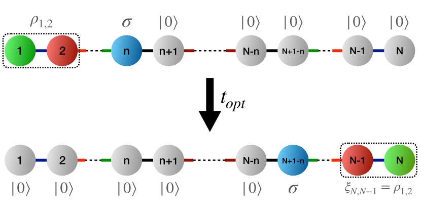
Figure 1: Perfect state transfer in $1D$ linear waveguide array. The system consists of $N$ modes interacting through modulated mirror-symmetric nearest-neighbor couplings. Any single-mode input state, $\sigma$ at mode $n$ as well as a multimode state, $\rho_{1,2}$ at modes $1$ and $2$ can be perfectly transferred, after evolution according to the Hamiltonian in Eq. (5) for $t=t_{\text{opt}}$, to the mode mirror-symmetric about the center of the arrangement (mode $N-n+1$ and modes $N-1,N$ respectively) as shown. PST requires the application of appropriate local phase gates at the receivers’ end, i.e., on the modes $N-n+1$, $N-1$, and $N$. Note that the intermodal non-input states that we consider to be in vacuum states can be initialized to any arbitrary CV state.

III One-dimensional waveguide array with mirror symmetry

It is well established that a lattice with unmodulated nearest-neighbor couplings cannot lead to perfect state transfer Christandl et al. (2004, 2005); Coutinho et al. (2023) unless it consists of only $2$ or $3$ nodes. Our goal now is to find a protocol that can allow us to transport an arbitrary CV state from one end of the waveguide, with $N\geq 3$ modes, to the other end with unit fidelity. Although PST has been demonstrated in spin systems for arbitrary qubit states, a similar analysis is missing in the continuous variable regime. Previous works have identified interactions that can perfectly transfer only a restricted class of single-mode states, e.g., path-entangled states Perez-Leija et al. (2013a), single photon states Perez-Leija et al. (2013b), and two-photon N$00$N states Swain and Rai (2021), but such systems cannot be used for the perfect transfer of other states such as coherent states Rai and Rai (2022). In this section, we construct a Hamiltonian with modulated nearest-neighbor couplings which makes the perfect transfer of any CV state possible across the length of a one-dimensional waveguide system.

We consider a model comprising $N$ identical waveguides arranged in an array and coupled to each other (see Fig. 1, with coupling strengths denoted by $J_{j}$ between adjacent modes $j$ and $j+1$). The coupling constants exhibit mirror symmetry between waveguide modes, i.e. $J_{j}=J_{N-j}$. The Hamiltonian that governs the $N$-mode system is given in Eq. (5), with $\mathcal{B}=N$ and $\mathcal{L}=\mathcal{H}=1$, where we represent $N=2m$ for even modes and $N=2m+1$ for odd modes, with $m$ being an integer taking values $1,2,3,\cdots$. We consider the coupling strength as

$$J_{j}=J\sqrt{\frac{j(N-j)}{N-1}},$$ (14)

with $j=0,1,2,...,m-1$ and $J$ being a constant, the value of which determines the optimal evolution time across the waveguide setup that allows for PST. We note that the coupling strength is motivated by the treatment given in Ref. Christandl et al. (2004), but with a normalization factor of $\sqrt{N-1}$. The additional factor ensures that the couplings do not assume very large values as the number of waveguide modes increases, which, in turn, facilitates their experimental implementation as we will discuss later.

Let us take an arbitrary $\mathcal{P}$-mode state as the input, with $\mathcal{P}\leq\lceil N/2\rceil$, where $\lceil N/2\rceil$ is the smallest integer greater than or equal to $N/2$. The final state of the system, upon evolution, is characterized by Eq. (11). Since the our waveguide lattice satisfies mirror symmetry about its center, it can support PST from any mode $j$ to the mode $N-j+1$. To see this, let us consider the expression for $\mathcal{A}_{j,N-j+1}$ which turns out to be

$$\mathcal{A}_{j,N-j+1} =\frac{(-i)^{N-1}}{2^{j}}\sin^{N-2j+1}\Big{(}\frac{Jt}{\sqrt{N-1}}\Big{)}\times$$ (15)

$$\Big{(}2^{j}+\sum_{r=1}^{j-1}(-2)^{r}c^{j,N}_{r}\cos^{2r}\frac{Jt}{\sqrt{N-1}}\Big{)},$$

where $j=1,2,\cdots,\lceil N/2\rceil$ and $c^{j,N}_{r}$ are integers. For the exemplary cases of $j=1,2,$ and $3$, the evolution coefficients have the form

$$\mathcal{A}_{1,N}=(-i)^{N-1}\sin^{N-1}\Big{(}\frac{Jt}{\sqrt{N-1}}\Big{)},$$ (16)

$$\mathcal{A}_{2,N-1}=\frac{(-i)^{N-1}}{4}\sin^{N-3}\Big{(}\frac{Jt}{\sqrt{N-1}}\Big{)}\times\Big{(}4-2(N-1)\cos^{2}\Big{(}\frac{Jt}{\sqrt{N-1}}\Big{)}\Big{)},$$ (17)

$$\mathcal{A}_{3,N-2}=\frac{(-i)^{N-1}}{8}\sin^{N-5}\Big{(}\frac{Jt}{\sqrt{N-1}}\Big{)}\times\Big{(}8+\sum_{r=1}^{2}(-2)^{r}\cos^{2r}\Big{(}\frac{Jt}{\sqrt{N-1}}\Big{)}\Big{(}\binom{N-2}{r}+N-2\Big{)}\Big{)},$$ (18)

and similarly for the other evolution coefficients. The form of the evolution coefficient clearly indicates that for PST, we must have

$$Jt_{\text{opt}}=(2n+1)\sqrt{N-1}\frac{\pi}{2}~{}~{}~{}\text{with}~{}n=0,1,\cdots$$ (19)

At $Jt_{\text{opt}}$, each evolution coefficient connecting mirror symmetric modes reduces to $\mathcal{A}_{j,N-j+1}=(-i)^{N-1}\implies|\mathcal{A}_{j,N-j+1}|=1$ as required for PST (all other elements in each row $j$ of the matrix $\mathcal{A}$ reduce to zero due to normalization). Therefore, the mode $j$ is transferred to the mode $N-j+1$, although it acquires a phase of $(-i)^{N-1}$. To complete the PST protocol, we propose the application of a local phase gate, given by $\hat{U}_{j}=\exp(i\phi_{N}\hat{a}_{j}^{\dagger}\hat{a}_{j})$ at each output port $j$. The phase gates at each mode for an $N$-mode waveguide array correspond to the application of the following phases:

$$\phi_{N}=\begin{cases}\pi~{}~{}\text{if}~{}~{}N=4m-1,\\ 0~{}~{}\text{if}~{}~{}N=4m+1,\\ \pi/2~{}~{}\text{if}~{}~{}N=4m+2,\\ 3\pi/2~{}~{}\text{if}~{}~{}N=4m.\\ \end{cases}$$ (20)

Therefore, given a $\mathcal{P}$-mode input state in a linear $N$-mode waveguide setup, PST is guaranteed to the mirror-symmetric modes upon evolution for $Jt_{\text{opt}}$ followed by the application of local phase gates at each output mode.

To demonstrate that our protocol indeed realizes PST, let us consider that the input is a single-mode Gaussian state at the first mode and the other $N-1$ modes are initialized as vacuum. The input state is characterized by the displacement vector and covariance matrix, given by

$$\mathbf{d}_{1}=\{\alpha_{x},\alpha_{y}\},$$ (21)

$$\Xi_{1}=\begin{pmatrix}a&b\\ b&c\end{pmatrix},$$ (22)

where $\alpha_{x},\alpha_{y},a,b,c$ are all real (for details on the phase-space formalism, see Appendix. A). The displacement vector and the covariance matrix pertaining to the modes $1$ and $N$ during the evolution are given as

$$\mathbf{d}_{1}=\cos^{N-1}\Big{(}\frac{Jt}{\sqrt{N-1}}\Big{)}\times\{\alpha_{x},\alpha_{y}\},$$ (23)

$$\Xi_{1}=\frac{1}{2}\begin{pmatrix}\cos^{2(N-1)}\Big{(}\frac{Jt}{\sqrt{N-1}}\Big{)}(a-1)+1&b\cos^{2(N-1)}\Big{(}\frac{Jt}{\sqrt{N-1}}\Big{)}\\ b\cos^{2(N-1)}\Big{(}\frac{Jt}{\sqrt{N-1}}\Big{)}&\cos^{2(N-1)}\Big{(}\frac{Jt}{\sqrt{N-1}}\Big{)}(c-1)+1\end{pmatrix},$$ (24)

$$\mathbf{d}_{N}=\sin^{N-1}\Big{(}\frac{Jt}{\sqrt{N-1}}\Big{)}\times\{\alpha_{x},\alpha_{y}\},$$ (25)

$$\Xi_{N}=\frac{1}{2}\begin{pmatrix}\sin^{2(N-1)}\Big{(}\frac{Jt}{\sqrt{N-1}}\Big{)}(a-1)+1&b\sin^{2(N-1)}\Big{(}\frac{Jt}{\sqrt{N-1}}\Big{)}\\ b\sin^{2(N-1)}\Big{(}\frac{Jt}{\sqrt{N-1}}\Big{)}&\sin^{2(N-1)}\Big{(}\frac{Jt}{\sqrt{N-1}}\Big{)}(c-1)+1\end{pmatrix}.$$ (26)

From Eqs. (23) - (26), it is evident that at $Jt_{\text{opt}}$, $\mathbf{d}_{1}$ and $\Xi_{1}$ reduce to those for vacuum whereas the mode $N$ is characterized by the displacement vector and covariance matrix of the input state, thereby indicating successful implementation of PST. In fact, at the optimal time, the $N$-mode state is described by the following first and second moments, after phase-gate application, as

$$\mathbf{d}_{f}=\{0,0,\cdots,0_{2N-2},\alpha_{x},\alpha_{y}\},$$ (27)

and $$\Xi_{f}=\frac{1}{2}\Bigg{[}\mathbb{I}^{\oplus N-1}\oplus\begin{pmatrix}a&b\\ b&c\end{pmatrix}\Bigg{]}.$$ (28)

The input state is taken to be Gaussian and since the evolution is governed by a quadratic Hamiltonian, the evolved state is also so. This allows us to derive the fidelity between the modes $1$ and $N$ during the evolution Mandarino et al. (2014) as

$$\mathcal{F}=\frac{2\exp-\frac{(1-\mathcal{A}_{N,1})^{2}\Big{(}(b\alpha_{x}^{2}-2c\alpha_{x}\alpha_{y}+a\alpha_{y}^{2})(1+\mathcal{A}_{N,1}^{2})+(\alpha_{x}^{2}+\alpha_{y}^{2})(1-\mathcal{A}_{N,1}^{2})\Big{)}}{(\chi_{+}-1)(1+\mathcal{A}_{N,1}^{2})+(1-\mathcal{A}_{N,1}^{2})}}{\sqrt{(\chi_{-})\mathcal{A}_{N,1}^{2}\Big{(}(a+b-2)+(\chi_{+}-a-b)\mathcal{A}_{N,1}^{2}\Big{)}}-\sqrt{(\chi_{+}+a+b)+(a+b)\chi_{-}\mathcal{A}_{N,1}^{2}+(\chi_{+}-a-b)(\chi_{+}-1)\mathcal{A}_{N,1}^{4}}},~{}~{}~{}~{}$$ (29)

where $\chi_{\pm}=ab-c^{2}\pm 1$. Eq. (29) becomes unity at $Jt_{\text{opt}}$. Therefore, with nearest-neighbor couplings defined by Eq. (14), any CV Gaussian state can be transferred with perfect fidelity through waveguide arrays comprising an arbitrary number of modes. Looking closely at Eq. (6) and using Eqs. (15), (19) and (20), one can show that the same happens for any arbitrary CV state, even if it is non-Gaussian.

Role of entanglement in perfect state transfer

It is established that a global entangling operation is necessary for the state transfer protocol. In fact, the evolution through a global Hamiltonian first makes the system (e.g., a lattice chain) genuinely multimode entangled, and then by utilizing that resource, the state is transported from the sender’s part to the receiver’s end, ultimately destroying the genuine multimode entanglement in the process. However, one-to-one correspondence between the fidelity of state transfer and the entanglement content of the system has not been established, so far.

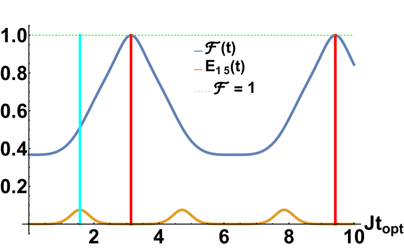
Figure 2: The behavior of fidelity and entanglement (ordinate) between the input and output modes of a five-mode linear waveguide setup with respect to the evolution parameters $Jt$ (abscissa). The fidelity $\mathcal{F}$ between the states at modes $1$ and $5$, is shown in blue (dark) solid curves, while orange (light) curves represent the logarithmic-negativity quantifying the entanglement $E_{15}(t)$, between the modes $1$ and $5$. Green (light) dashed horizontal line shows PST (unit fidelity). The vertical lines identify the values of $Jt=\pi,3\pi$ (dark red vertical solid line) and $Jt=\pi/2$ (light blue vertical solid line) where the fidelity becomes equal to $1$ and $1/2$ respectively and consequently, the entanglement vanishes and reaches its maximum value. Both axes are dimensionless.

We analyze the relationship between the dynamics of entanglement shared in the input and output modes and the fidelity. For brevity, we restrict our attention to linear waveguides and the transfer of a single-mode Gaussian state, although qualitatively similar results would hold for multimode CV states, even for non-Gaussian ones. Our treatment focuses on the first and last modes of a linear $N$-mode waveguide arrangement whose evolution is driven by the Hamiltonian in Eq. (5). In order to estimate the entanglement, $E_{1N}(t)$ between the input and the output modes during the dynamics, we compute logarithmic negativity Serafini (2017), via covariance matrix corresponding to the two-mode state $\rho_{1N}(t)=\Tr_{2,3,\cdots,N-1}\rho(t)$. With the initial state characterized by Eqs. (21) and (22) and considering the remaining modes to be initialized in vacuum, the covariance matrix of $\rho_{1N}(t)$ can be represented as

$$\Xi_{1N}=\begin{pmatrix}\Xi_{1}&\Xi\\ \Xi&\Xi_{N}\end{pmatrix},~{}~{}\text{where}~{}~{}$$ (30)

$$\Xi=\frac{\sin\Big(2Jt/\sqrt{N-1}\Big{missing})^{N-1}}{2^{N-1}}\begin{pmatrix}a-1&b\\ b&c-1\end{pmatrix},$$ (31)

and we make use of Eqs. (23) through (26). We consider $N=5$ and the input state parameters as $\alpha_{x}=\alpha_{y}=1,a=2,b=\sqrt{5},c=3$, thereby computing the logarithmic negativity and the fidelity according to Eq. (29). We notice that the entanglement between the sender (mode $1$) and the receiver (mode $5$) modes vanishes when PST occurs at $Jt=Jt_{\text{opt}}=(2n+1)\pi$, whereas it becomes maximum at $Jt_{\text{opt}}/2$ as depicted in Fig. 2. This indicates that at the optimal instant, the input and output modes constitute a separable state, a condition that we have argued earlier to be necessary for PST, although entanglement is also a key ingredient that occurs during evolution. Let us also mention here that our results bear a striking resemblance to those in Ref. Qian et al. (2005), obtained for discrete systems, where the entanglement is quantified by the mirror-mode concurrence (which is the sum of the concurrence corresponding to each pair of mirror-symmetric modes) but exhibits the exact same qualitative behavior with respect to the fidelity at $Jt_{\text{opt}}$ and $Jt_{\text{opt}}/2$, even though we consider the logarithmic negativity between the input and the output modes only, regardless of the remaining intermediate modes. Therefore, it can be argued that modal entanglement is certainly responsible for the successful transfer of arbitrary states through the QST process.

IV PST leading to mirror-mode swap operation

Conventionally, in the state transfer protocol, the modes of the waveguide setup (excluding the input mode) are initially considered to be in the vacuum state. However, even with no input provided, the waveguide modes are not expected to be in the vacuum state and as such need to be engineered to $\ket{0}$. Since the Hamiltonian in Eq. (5) together with appropriate phase gates can perfectly transfer states between modes $j$ and $N-j+1$, we can also employ our protocol to realize SWAP gates between the aforementioned modes. In this case, it is evident that the user must have access to all the waveguide modes since the states to be interchanged must be provided apriori to the evolution.

Let us consider that the modes $2$ to $N$ in the network are initialized with any arbitrary Gaussian state which can be characterized by the displacement vector and covariance matrix as

$$\mathbf{d}_{\text{in}}=\{\alpha_{x},\alpha_{y}\}^{T}\oplus_{i=2}^{N}\{\beta_{xi},\beta_{yi}\}^{T},$$

and $$\Xi_{\text{in}}=\begin{pmatrix}a&b\\ b&c\end{pmatrix}\oplus_{i=2}^{N}\begin{pmatrix}p_{i}&q_{i}\\ q_{i}&s_{i}\end{pmatrix},$$ (32)

where $\{\alpha_{x},\alpha_{y}\}^{T}$ corresponds to the displacement vector of the input mode and $\{\beta_{xi},\beta_{yi}\}^{T}$ denotes the displacement vector of the arbitrary state in mode $i$. Similarly, $a,b,$ and $c$ are the elements of the covariance matrix pertaining to the input state, whereas $p_{i},q_{i}$ and $s_{i}$ stand for the same in the case of the state in mode $i$. Now, upon evolution through an $N$-mode waveguide characterized by a Hamiltonian with nearest-neighbor couplings defined in Eq. (14), the final state at $Jt_{\text{opt}}=\sqrt{N-1}\frac{\pi}{2}$ followed by the application of corresponding phase gates, as prescribed in Eq. (20), in all the modes, is described by

$$\mathbf{d}_{f}=\oplus_{i=1}^{N-1}\times\{\beta_{xi},\beta_{yi}\}^{T}\oplus\{\alpha_{x},\alpha_{y}\}^{T},$$

$$\Xi_{f}=\oplus_{i=1}^{N-1}\begin{pmatrix}p_{N-i+1}&q_{N-i+1}\\ q_{N-i+1}&s_{N-i+1}\end{pmatrix}\oplus\begin{pmatrix}a&b\\ b&c\end{pmatrix},$$ (33)

which clearly illustrates that $\Xi_{f}$ is just a mirror-inverted version of $\Xi_{\text{in}}$ about the central mode when the total number of modes is odd ($N=2m+1$) or about the central coupling when the total number of modes is even ($N=2m$). Note that the protocol still goes through for any arbitrary initialization and Gaussian states are taken to illustrate the fact in the phase space formalism. Thus, by applying local phase shifts in all the modes, one can realize the SWAP operations between mirror-symmetric modes by evolving the system for a period of $(0,t_{\text{opt}})$. Therefore, if required states are provided in specific modes, a collateral benefit of the optimal PST Hamiltonian is to act as a SWAP operator between modes that are equispaced from the center of the waveguide array. This, however, incurs the cost of local phase shifters in each mode, unlike the PST process where only the output mode(s) need to be phase-shifted.

Remark: Let us consider that the initial state of an $N$-mode system is $\oplus_{j=1}^{N}|\psi^{j}\rangle_{j}=\oplus_{j=1}^{N}\Big{(}\sum_{n_{k}=0}^{\infty}C^{j}_{n_{k}}|n_{k}\rangle_{j}\Big{)}$, where the superscript $j$ represents the state label, while $j$ in the subscript denotes the mode at which it is present, and $\ket{n_{k}}$ is the state containing $n_{k}$ number of photons. Upon evolution up to the optimal time and further implementation of local phase-shifts, the final state reduces to $\oplus_{j=1}^{N}\Big{(}\sum_{n_{k}=0}^{\infty}C^{j}_{n_{k}}|n_{k}\rangle_{N-j+1}\Big{)}=\oplus_{j=1}^{N}|\psi^{j}\rangle_{N-j+1}$, which is a consequence of $|\mathcal{A}_{j,N-j+1}|=1~{}~{}\forall~{}~{}j$ (a condition that depends on the Hamiltonian in action and not on the initialization of the lattice). Therefore, mirror-mode SWAP operation can be implemented for a collection of arbitrary CV states.

V PST in higher dimensional lattices

Going beyond one-dimensional systems, we demonstrate how PST of any arbitrary CV state can be implemented on two-dimensional ($2$D) and three-dimensional ($3$D) waveguide lattices. We use the PST Hamiltonian in (5) to derive the evolution which would lead to PST from one part to another of a waveguide setup arranged in $2D$ and $3D$. Accurate transfer of a CV state in a higher dimensional lattice would allow us to realize state transfer across several modes in a more compact manner since distant transfer along a linear array would require a very long chain of waveguide modes.

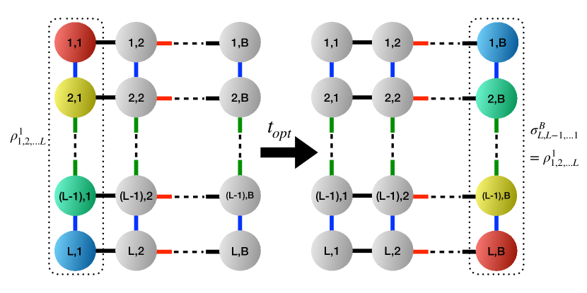
Figure 3: Two-dimensional lattice of waveguide modes supporting PST. The arrangement consists of $\mathcal{L}$ rows and $\mathcal{B}$ columns, with modulated nearest-neighbor couplings which are mirror symmetric. Each available mode is denoted as $i,j$. The input state, $\rho^{1}_{1,2,...,L}$ at the modes $1,1$ to $1,L$ can be a separable or entangled $L$-mode state, and the remaining modes are initialized with the vacuum states, but can be taken to be any arbitrary state. Suitable local phase gates, following the evolution under the specified Hamiltonian for time $t_{opt}$, must be implemented at the receivers’ end (at the far right side) in order to accomplish PST - when the output state $\sigma^{\mathcal{B}}_{1,2,\cdots,L}$ at the modes $1,\mathcal{B}$ to $\mathcal{L},\mathcal{B}$ (which are mirror-symmetrically opposite to the input modes about the center of the geometry) becomes exactly the same as the input one, thereby leading to PST.

We define our coordinate system as follows. $\mathcal{L}$ and $\mathcal{B}$ modes along two orthogonal directions comprise a $2D$ latttice on a plane. Along the direction perpendicular to the plane, we consider $\mathcal{H}$ number of waveguide modes when in $3D$.

V.0.1 PST in two-dimensional waveguide lattice

Let us first concentrate on a rectangular cluster with $\mathcal{L}$ rows and $\mathcal{B}$ columns, as illustrated in Fig. 3. Therefore, the total number of modes supported by the entire structure is $N=\mathcal{L}\times\mathcal{B}$. Evidently, we can consider each row as an $\mathcal{B}$-mode linear waveguide chain, which is coupled to another linear pattern of $\mathcal{B}$ waveguide modes. Conversely, an $\mathcal{L}$-mode linear waveguide setup describes every column of the rectangular system. Every mode within the lattice is linked with four other modes, except for the modes at the boundaries and corners, which have a coordination number of $3$ and $2$ respectively. The Hamiltonian governing the PST protocol is $\hat{H}^{\mathcal{L},\mathcal{B}}=\hat{H}^{\mathcal{L}}+\hat{H}^{\mathcal{B}}$ where

$$\hat{H}^{\mathcal{L}}=\sqrt{\frac{\mathcal{L}-1}{\mathcal{B}-1}}\sum_{j,k=1}^{\mathcal{L}-1,\mathcal{B}}J^{\mathcal{L}}_{j}(\hat{a}_{(j,k)}^{\dagger}\hat{a}_{(j+1,k)}+\hat{a}_{(j,k)}\hat{a}_{(j+1,k)}^{\dagger}),~{}~{}~{}~{}~{}~{}$$ (34)

$$\text{and}~{}~{}\hat{H}^{\mathcal{B}}=\sum_{j,k=1}^{\mathcal{L},\mathcal{B}-1}J^{\mathcal{B}}_{k}(\hat{a}_{(j,k)}^{\dagger}\hat{a}_{(j,k+1)}+\hat{a}_{(j,k)}\hat{a}_{(j,k+1)}^{\dagger}).$$ (35)

Evidently, the Hamiltonian to realize PST in a $2D$ lattice comprises a Hamiltonian for $\mathcal{L}$ number of modes, whose interaction strength is scaled by a factor of $\sqrt{\frac{\mathcal{L}-1}{\mathcal{B}-1}}$, and another one-dimensional Hamiltonian corresponding to $\mathcal{B}$ modes. Setting $J^{\mathcal{B}}_{k}$ and $J^{\mathcal{L}}_{j}$ satisfying Eq. (14), one can realize PST from the mode $(i,j)$ to the mode $(\mathcal{L}-i+1,\mathcal{B}-j+1)$ at the mirror-symmetric position of the waveguide composition aided with local phase gates at the output modes.

The evolution coefficients, involving mirror-symmetric sites, and the optimal time bear resemblance to the ones for the linear chain, as

$$\mathcal{A}_{(j,k),(\mathcal{L}-j+1,\mathcal{B}-k+1)}=\mathcal{A}_{j,\mathcal{L}-j+1}\times\mathcal{A}_{k,\mathcal{B}-k+1}$$ (36)

$$\text{with}~{}~{}Jt_{\text{opt}}=(2n+1)\sqrt{\mathcal{B}-1}\frac{\pi}{2}~{}~{}(n=0,1,\cdots,).~{}~{}~{}~{}~{}~{}$$ (37)

The fact that the evolution coefficient in the case of a $2D$ waveguide system can be factored into a product of the same in each involved direction follows from the property that the state transfer proceeds independently in separate dimensions Kay (2010). Note that the evolution coefficients must be evaluated according to Eqs. (34) and (35). This would lead to expressions for $\mathcal{A}_{j,\mathcal{L}-j+1}$ and $\mathcal{A}_{k,\mathcal{B}-k+1}$ with functional forms similar to Eq. (15) but with arguments scaled by the aforementioned factor, if any. Moreover, the phase acquired by each output mode during evolution is $(-i)^{\mathcal{L}+\mathcal{B}-2}$ in the case of a $2D$ waveguide lattice. Therefore, the phase gates to be provided at the output modes correspond to implementing a correction phase given by

$$\phi_{\mathcal{L}\mathcal{B}}=\begin{cases}\pi/2~{}~{}\text{if}~{}~{}\mathcal{L}+\mathcal{B}=4m-1\\ 3\pi/2~{}~{}\text{if}~{}~{}\mathcal{L}+\mathcal{B}=4m+1\\ 0~{}~{}\text{if}~{}~{}\mathcal{L}+\mathcal{B}=4m+2\\ \pi~{}~{}\text{if}~{}~{}\mathcal{L}+\mathcal{B}=4m.\\ \end{cases}$$ (38)

It is thus clear that PST occurs from the site $(j,k)$ to the mode at site $(\mathcal{L}-j+1,\mathcal{B}-k+1)$ when the evolution is executed for an optimal time given in Eq. (37) followed by a phase shift at the output modes. Therefore, applying the PST Hamiltonian for linear waveguide setups, one can also achieve the transfer of any arbitrary state, across a $2D$ rectangular lattice, with unit fidelity, notwithstanding the initialization of the non-input modes in the waveguide. If a multimode (say, $\mathcal{P}$ mode) CV state, be it pure or mixed, Gaussian or non-Gaussian, is to be transmited, it would be transferred perfectly to the $\mathcal{P}$ mirror-symmetric modes at the output. With all the $\mathcal{P}$ output modes being accessible, the application of phase gates, which is essential to achieve unit fidelity, can also be easily applied. Furthermore, $\hat{H}^{\mathcal{L}\mathcal{B}}$ also acts as a SWAP gate between modes $(j,k)$ and $(\mathcal{L}-j+1,\mathcal{B}-k+1)$ when local phase gates are applied in all the modes in the lattice as discussed in the previous section. As a result, the Hamiltonian governing PST in a $2D$ arrangement of waveguide modes retains all the beneficial properties of that concerning linear PST.

V.0.2 Three-dimensional waveguide arrangement for PST

The Hamiltonian which supports the perfect transfer of any arbitrary multimode CV state across a $3D$ geometry can be written as $\hat{H}^{\mathcal{L}\mathcal{B}\mathcal{H}}=\hat{H}^{\mathcal{L}}+\hat{H}^{\mathcal{B}}+\hat{H}^{\mathcal{H}}$ with

$$\hat{H}^{\mathcal{H}}=\sqrt{\frac{\mathcal{H}-1}{\mathcal{B}-1}}\sum_{j,k,l=1}^{\mathcal{L},\mathcal{B},\mathcal{H}-1}J^{\mathcal{H}}_{l}(\hat{a}_{(j,k,l)}^{\dagger}\hat{a}_{(j,k,l+1)}+\hat{a}_{(j,k,l)}\hat{a}_{(j,k,l+1)}^{\dagger}),~{}~{}~{}~{}~{}~{}$$ (39)

and $\hat{H}^{\mathcal{L}}$ and $\hat{H}^{\mathcal{B}}$ given by Eqs. (34) and (35) where the summations run over the three indices $j,k,l$ along the three-dimensions. The waveguide arrangement contains a total number of modes equal to $N=\mathcal{L}\mathcal{B}\mathcal{H}$. Akin to the two-dimensional QST protocol, the evolution of the system is independent in each dimension and we can once more write down the evolution coefficient as a product of the same in each direction. Evaluating the evolution coefficients corresponding to $\hat{H}^{\mathcal{L}},\hat{H}^{\mathcal{B}},$ and $\hat{H}^{\mathcal{H}}$, it is easy to see that in $3D$, the optimal evolution coefficient is $\mathcal{A}_{(j,k,l),(\mathcal{L}-j+1,\mathcal{B}-k+1,\mathcal{H}-l+1})=\mathcal{A}_{j,\mathcal{L}-j+1}\times\mathcal{A}_{k,\mathcal{B}-k+1}\times\mathcal{A}_{l,\mathcal{H}-l+1}~{}~{}\text{with}~{}~{}Jt_{\text{opt}}=(2n+1)\sqrt{\mathcal{B}-1}\frac{\pi}{2}~{}~{}\text{for}~{}~{}(n=0,1,\cdots,)$. It is observed that evolving the initial system for the optimal time reduces each $\mathcal{A}_{(j,k,l),(\mathcal{L}-j+1,\mathcal{B}-k+1,\mathcal{H}-l+1)}~{}~{}\text{to}~{}~{}(-i)^{\mathcal{L}+\mathcal{B}+\mathcal{H}-3}$ which represents the local phase acquired by each mode. This calls for the application of phase gates at the output sites corresponding to

$$\phi_{\mathcal{L}\mathcal{B}\mathcal{H}}=\begin{cases}\pi/2~{}~{}\text{if}~{}~{}\mathcal{L}+\mathcal{B}+\mathcal{H}=4m,\\ 3\pi/2~{}~{}\text{if}~{}~{}\mathcal{L}+\mathcal{B}+\mathcal{H}=4m+2,\\ 0~{}~{}\text{if}~{}~{}\mathcal{L}+\mathcal{B}+\mathcal{H}=4m-1,\\ \pi~{}~{}\text{if}~{}~{}\mathcal{L}+\mathcal{B}+\mathcal{H}=4m+1,\\ \end{cases}$$ (40)

as the correction phase, in order to ensure state transfer to the mirror-symmetric output modes with unit fidelity. Similar to the cases in $1D$ and $2D$, the application of proper local phase shifts in all the waveguide modes can help to use the Hamiltonian in implementing a SWAP gate between modes $(j,k,l)$ and $(\mathcal{L}-j+1,\mathcal{B}-k+1,\mathcal{H}-l+1)$. Therefore, if the condition for PST is satisfied by $\hat{H}^{\mathcal{L}\mathcal{B}\mathcal{H}}$, evolution through $t=0\rightarrow t_{\text{opt}}$ followed by local phase gates can ensure the realization of PST as well as mirror-mode SWAP operation of any multimode CV state, irrespective of its Gaussian (non-Gaussian) character and purity.

Possible experimental implementation of PST Hamiltonian

Optical lattices serve as a potential framework for realizing tight-binding Hamiltonians Christodoulides et al. (2003); Longhi (2009); Szameit and Nolte (2010) for large-scale quantum information processing Politi et al. (2008). Thus, our proposed Hamiltonian, belonging to the tight-binding class can be implemented in waveguide arrays which, moreover, admit negligible photon interactions, provide long coherence times, and also allow for high experimental control Owens et al. (2011). A mode-dependent coupling strength, like the one we present for our purpose, can be engineered by suitably manipulating the waveguide separation Szameit and Nolte (2010). In fact, for each $J_{j}$ as defined in Eq. (14), (with additional factors in $2D$ and $3D$), the optimal separation $\kappa_{j}$ between waveguide modes $j$ and $j+1$, in the weak coupling limit, can be doctored according to

$$\kappa_{j}=\eta^{-1}\Big{(}\ln\frac{\gamma}{J}-\ln\frac{J_{j}}{J}\Big{)},$$ (41)

where $\gamma$, and $\eta$ are parameters depending on the particular setup Bellec et al. (2012) and $J$ as defined in Eq. (14). Note that the above formalism is applicable only when the coupling strengths between the adjacent modes are small, which is ensured since each $J_{j}$ is scaled by $1/\sqrt{N-1}$, i.e., for large $N$, even though the numerator in Eq. (14) increases, so does the scaling factor and the coupling strengths remain experimentally manageable. It is interesting to mention here that diffraction losses occurring in any waveguide array due to lattice truncation and edge effects Longhi (2010) can be readily minimized by engineering the coupling coefficients Gordon (2004); Keil et al. (2012) which is the essence of our PST protocol. As shown in reference Fukuda et al. (2004), negligible propagation defects make waveguide structures a feasible breadboard for implementing the PST Hamiltonian effectively.

VI Conclusion

In a quantum computing circuit, state transfer can be a crucial component for propagating quantum information from one quantum processor to another. The information transmitted should also be as little distorted as possible, to ensure smooth functioning of the network. On the other hand, quantum state transmission is also an integral part of quanutum communication networks. Therefore, finding an optimal protocol for perfect quantum transfer (PST) is one of the demanding issues in both the domains of quantum computers and quantum communication.

We demonstrated the perfect transfer of any given continuous variable (CV) quantum state through an optical waveguide lattice governed by a Hamiltonian comprising modulated nearest-neighbor couplings. In particular, we found a criterion that should be met by any Hamiltonian required during evolution in order to accurately transfer an arbitrary state from one part to another in an optical waveguide array. There are several contributions in the literature on PST in CV systems, but all of them are limited to a specific kind of state transfer, e.g., some of the studies are limited to the perfect transfer of single- and two-photon Fock states, or pure path entangled states. The perfect transfer of non-classical properties such as squeezing strength as well as average photon number has also been reported Rai and Rai (2022). It is important to note, however, that transmitting photon numbers accurately does not translate into PST, since two states differing by local phases can have the same mean number of photons. This is significant since such states are essentially different from each other since they can carry vastly different information.

In this work, we went beyond the aforementioned restrictions and studied the PST of a generic multimode CV state, which may be pure or mixed implying irrevocably precise transfer of the encoded information. Our proposed protocol, with mirror-symmetric Hamiltonian and the subsequent application of specific phase-shifts, can further allow for the relocation of any CV state between the two mirror-symmetric of a waveguide setup in two- as well as three-dimensions, with unit fidelity, upon evolution up to some optimal time. Our protocol demands the application of local phase shifts at the output modes, the correction phase being dependent on the total number of modes comprising the waveguide setup. We argued that this local manipulation is allowed since the input and output modes are always accessible in a PST experiment. In addition, we showed that with the help of local phase unitaries in all the waveguide modes, a mirror-mode swapping of states can be achieved as a collateral benefit of our engineering. One of the main features of our work is that we do not need to bother about the initial state of modes other than the input ones. Indeed, any initialization of the system (other than the sender mode) can accomplish PST. We further looked into how the entanglement between the sender and the receiver modes of the linear waveguide array is related to the efficiency of the protocol. More precisely, we noted that the aforementioned entanglement is maximum at half the time taken to achieve PST, whereas it vanishes at the instant of PST. This showed how entanglement is an indispensable component for the success of the protocol, in which the assistance of entanglement is still present.

Our work extends the theory of continuous-variable state transfer to bring all continuous-variable states under one umbrella. Our protocol is experimentally feasible, as argued in our manuscript, and would lead to the successful implementation of several information theoretic protocols driven by linear optical elements O’Brien (2007), which rely on state transfer.

Appendix A CV-systems - a brief discussion on the phase-space formalism

Characterized by quadrature variables, such as $\hat{x}$ and $\hat{p}$, which are canonically conjugate with each other, continuous variable systems possess an infinite spectrum Serafini (2017); Braunstein and van Loock (2005). The Hamiltonian of an $N$-mode system comprising $2N$ parameters, $\{\hat{x}_{k},\hat{p}_{k}\}$ (with $k=1,2,\dots,N$), is defined as

$$\hat{H}=\frac{1}{2}\sum_{k=1}^{N}(\hat{x}_{k}^{2}+\hat{p}_{k}^{2})=\sum_{k=1}^{N}\Big{(}\hat{a}_{k}^{\dagger}\hat{a}_{k}+\frac{1}{2}\Big{)},$$ (42)

where $\hat{a}_{k}^{\dagger}$ and $\hat{a}_{k}$ are the creation and annihilation operators respectively for the mode $k$ and, in terms of the quadrature variables, they are given by

$$\hat{a}_{k}=\frac{\hat{x}_{k}+i\hat{p}_{k}}{\sqrt{2}},~{}~{}~{}~{}~{}~{}~{}\text{and}~{}~{}~{}~{}~{}~{}\hat{a}_{k}^{\dagger}=\frac{\hat{x}_{k}-i\hat{p}_{k}}{\sqrt{2}},$$ (43)

with $i=\sqrt{-1}$. The bosonic commutation relation, $[\hat{a}_{k}^{\dagger},\hat{a}_{k}]=-1$, is obeyed by the creation and annihilation operators for any mode. The quadrature vector, $\hat{R}=(\hat{x}_{1},\hat{p}_{1},\dots,\hat{x}_{N},\hat{p}_{N})^{T}$, helps to rewrite the commutation relation as

$$\left[\hat{R}_{k},\hat{R}_{l}\right]=i\mathcal{W}_{kl}\quad\text{with}~{}~{}\mathcal{W}=\bigoplus\limits_{j=1}^{\mathcal{N}}\Omega_{j}.$$ (44)

Here, $\mathcal{W}$ represents the $\mathcal{N}$-mode symplectic form, and $\Omega_{j}$ is given by

$$\quad\Omega_{j}=\begin{pmatrix}0&1\\ -1&0\end{pmatrix}\forall j.$$ (45)

Gaussian states are the most widely studied class of CV states Ferraro et al. (2005); Weedbrook et al. (2012). Being the ground and thermal states of Hamiltonians which are at most quadratic functions of the quadrature variables, a Gaussian state, $\rho$, can be completely characterized by their first and second moments, quantified respectively by the $2N$-element displacement vector $\mathbf{d}$ and the $2N\times 2N$ dimensional covariance matrix, $\Xi$, in the following way:

$$d_{k}=\expectationvalue{\hat{R}_{k}}_{\rho},$$ (46)

$$\Xi_{kl} =\frac{1}{2}\expectationvalue{\hat{R}_{k}\hat{R}_{l}+\hat{R}_{l}\hat{R}_{k}}_{\rho}-\expectationvalue{\hat{R}_{k}}_{\rho}\expectationvalue{\hat{R}_{l}}_{\rho}.$$ (47)

Here, $\Xi$ is a real, symmetric, and positive definite matrix. Gaussian dynamics is governed similarly by second-order Hamiltonians. In the symplectic formalism, any $N$-mode quadratic Hamiltonian $\hat{\mathcal{H}}$ can be written as $\hat{\mathcal{H}}=\frac{1}{2}\hat{\xi}^{\dagger}\hat{H}\hat{\xi}$ with $\hat{\xi}=\left(\hat{a}_{1},\hat{a}_{2},...,\hat{a}_{N},\hat{a}_{1}^{\dagger},...,\hat{a}_{N}^{\dagger}\right)^{T}$. We can construct the symplectic matrix $S_{H}$ as Luis and Sanchez-Soto (1995); Arvind. et al. (1995); Adesso et al. (2014)

$$S_{H}=T^{\dagger}L^{\dagger}\exp{-iK\hat{H}}LT,$$ (48)

where $K,L$ and $T$ are $2N\times 2N$ matrices given by

$$K=\begin{pmatrix}\mathbb{I}_{N}&\mathbb{O}_{N}\\ \mathbb{O}_{N}&-\mathbb{I}_{N}\end{pmatrix},$$ (49)

$$L=\frac{1}{\sqrt{2}}\begin{pmatrix}\mathbb{I}_{N}&i\mathbb{I}_{N}\\ \mathbb{I}_{N}&-i\mathbb{I}_{N}\end{pmatrix},$$ (50)

$$T_{jk}=\delta_{k,2j-1}+\delta_{k+2N,2j},$$ (51)

with $\mathbb{I}_{N}$ being the $N$-dimensional identity and $\mathbb{O}_{N}$ being the null matrix. The evolved Gaussian state, in terms of its displacement vector and covariance matrix, can be characterized as Adesso et al. (2014)

$$\rho^{\prime}=e^{-i\hat{H}t}\rho e^{i\hat{H}t}\equiv \mathbb{d}^{\prime}=S_{H}\mathbb{d},$$ (53)

$$\Xi^{\prime}=S_{H}\Xi S_{H}^{T},$$

where the evolution is governed by $\hat{H}$ in Eq. (42) and since the evolved state also remains Gaussian, it can be represented by displacement and covariance matrix of the initial state via $S_{H}$ in Eq. (48)

References

- Plenio et al. (2004) M. B. Plenio, J. Hartley, and J. Eisert, New Journal of Physics 6, 36 (2004).
- Nielsen and Chuang (2010) M. A. Nielsen and I. L. Chuang, Quantum Computation and Quantum Information: 10th Anniversary Edition (Cambridge University Press, 2010).
- Bennett et al. (1993) C. H. Bennett, G. Brassard, C. Crépeau, R. Jozsa, A. Peres, and W. K. Wootters, Phys. Rev. Lett. 70, 1895 (1993).
- Cirac et al. (1997) J. I. Cirac, P. Zoller, H. J. Kimble, and H. Mabuchi, Phys. Rev. Lett. 78, 3221 (1997).
- Kielpinski et al. (2002) D. Kielpinski, C. Monroe, and D. J. Wineland, Nature 417, 709 (2002).
- Seidelin et al. (2006) S. Seidelin, J. Chiaverini, R. Reichle, J. J. Bollinger, D. Leibfried, J. Britton, J. H. Wesenberg, R. B. Blakestad, R. J. Epstein, D. B. Hume, W. M. Itano, J. D. Jost, C. Langer, R. Ozeri, N. Shiga, and D. J. Wineland, Phys. Rev. Lett. 96, 253003 (2006).
- Wallraff et al. (2004) A. Wallraff, D. I. Schuster, A. Blais, L. Frunzio, R.-. S. Huang, J. Majer, S. Kumar, S. M. Girvin, and R. J. Schoelkopf, Nature 431, 162 (2004).
- Majer et al. (2007) J. Majer, J. M. Chow, J. M. Gambetta, J. Koch, B. R. Johnson, J. A. Schreier, L. Frunzio, D. I. Schuster, A. A. Houck, A. Wallraff, A. Blais, M. H. Devoret, S. M. Girvin, and R. J. Schoelkopf, Nature 449, 443 (2007).
- Herskind et al. (2009) P. F. Herskind, A. Dantan, J. P. Marler, M. Albert, and M. Drewsen, Nature Physics 5, 494 (2009).
- Paik et al. (2011) H. Paik, D. I. Schuster, L. S. Bishop, G. Kirchmair, G. Catelani, A. P. Sears, B. R. Johnson, M. J. Reagor, L. Frunzio, L. I. Glazman, S. M. Girvin, M. H. Devoret, and R. J. Schoelkopf, Phys. Rev. Lett. 107, 240501 (2011).
- Benenti et al. (2004) G. Benenti, G. Casati, and G. Strini, Principles of Quantum Computation and Information (WORLD SCIENTIFIC, 2004) https://www.worldscientific.com/doi/pdf/10.1142/5528 .
- Schoelkopf and Girvin (2008) R. J. Schoelkopf and S. M. Girvin, Nature 451, 664 (2008).
- Bose (2003) S. Bose, Phys. Rev. Lett. 91, 207901 (2003).
- Burgarth et al. (2005) D. Burgarth, V. Giovannetti, and S. Bose, Journal of Physics A: Mathematical and General 38, 6793 (2005).
- Burgarth and Bose (2005a) D. Burgarth and S. Bose, New Journal of Physics 7, 135 (2005a).
- Burgarth and Bose (2005b) D. Burgarth and S. Bose, Phys. Rev. A 71, 052315 (2005b).
- Burgarth (2007) D. Burgarth, (2007), https://doi.org/10.48550/arXiv.0704.1309.
- Yung and Bose (2005) M. Yung and S. Bose, Phys. Rev. A 71, 032310 (2005).
- Devitt et al. (2013) S. J. Devitt, W. J. Munro, and K. Nemoto, Reports on Progress in Physics 76, 076001 (2013).
- Raussendorf and Briegel (2001) R. Raussendorf and H. J. Briegel, Phys. Rev. Lett. 86, 5188 (2001).
- Zhou et al. (2002) X. Zhou, Z. Zhou, G. Guo, and M. J. Feldman, Phys. Rev. Lett. 89, 197903 (2002).
- Benjamin and Bose (2004) S. C. Benjamin and S. Bose, Phys. Rev. A 70, 032314 (2004).
- Kay (2008) A. Kay, Phys. Rev. A 78, 012346 (2008).
- Mkrtchian (2008) G. F. Mkrtchian, Physics Letters A 372, 5270 (2008).
- Lyakhov and Bruder (2005) A. Lyakhov and C. Bruder, New Journal of Physics 7, 181 (2005).
- Lyakhov and Bruder (2006) A. O. Lyakhov and C. Bruder, Phys. Rev. B 74, 235303 (2006).
- Romito et al. (2005) A. Romito, R. Fazio, and C. Bruder, Phys. Rev. B 71, 100501 (2005).
- Tsomokos et al. (2007) D. I. Tsomokos, M. J. Hartmann, S. F. Huelga, and M. B. Plenio, New Journal of Physics 9, 79 (2007).
- D’Amico (2005) I. D’Amico, (2005), https://doi.org/10.48550/arXiv.cond-mat/0511470.
- Spiller et al. (2007) T. Spiller, I. D’Amico, and B. W. Lovett, New Journal of Physics 9, 20 (2007).
- Zhang et al. (2005) J. Zhang, G. L. Long, W. Zhang, Z. Deng, W. Liu, and Z. Lu, Phys. Rev. A 72, 012331 (2005).
- Zhang et al. (2006) J. Zhang, X. Peng, and D. Suter, Phys. Rev. A 73, 062325 (2006).
- Fitzsimons et al. (2007) J. Fitzsimons, L. Xiao, S. C. Benjamin, and J. A. Jones, Phys. Rev. Lett. 99, 030501 (2007).
- Rao et al. (2014) K. R. K. Rao, T. S. Mahesh, and A. Kumar, Phys. Rev. A 90, 012306 (2014).
- Paternostro et al. (2005) M. Paternostro, G. M. Palma, M. S. Kim, and G. Falci, Phys. Rev. A 71, 042311 (2005).
- Almeida et al. (2016) G. M. A. Almeida, F. Ciccarello, T. J. G. Apollaro, and A. M. C. Souza, Phys. Rev. A 93, 032310 (2016).
- Sillanpää et al. (2007) M. A. Sillanpää, J. I. Park, and R. W. Simmonds, Nature 449, 438 (2007).
- Togan et al. (2010) E. Togan, Y. Chu, A. S. Trifonov, L. Jiang, J. Maze, L. Childress, M. V. G. Dutt, A. S. Sørensen, P. R. Hemmer, A. S. Zibrov, and M. D. Lukin, Nature 466, 730 (2010).
- You and Nori (2011) J. Q. You and F. Nori, Nature 474, 589 (2011).
- Schmidt-Kaler et al. (2003) F. Schmidt-Kaler, H. Häffner, M. Riebe, S. Gulde, G. P. T. Lancaster, T. Deuschle, C. Becher, C. F. Roos, J. Eschner, and R. Blatt, Nature 422, 408 (2003).
- Leibfried et al. (2003) D. Leibfried, B. DeMarco, V. Meyer, D. Lucas, M. Barrett, J. Britton, W. M. Itano, B. Jelenković, C. Langer, T. Rosenband, and D. J. Wineland, Nature 422, 412 (2003).
- Uhlmann (1976) A. Uhlmann, Reports on Mathematical Physics 9, 273 (1976).
- Jozsa (1994) R. Jozsa, Journal of Modern Optics 41, 2315 (1994).
- Albanese et al. (2004) C. Albanese, M. Christandl, N. Datta, and A. Ekert, Phys. Rev. Lett. 93, 230502 (2004).
- Christandl et al. (2005) M. Christandl, N. Datta, T. C. Dorlas, A. Ekert, A. Kay, and A. J. Landahl, Phys. Rev. A 71, 032312 (2005).
- Kay (2006) A. Kay, Phys. Rev. A 73, 032306 (2006).
- Di Franco et al. (2008) C. Di Franco, M. Paternostro, and M. S. Kim, Phys. Rev. Lett. 101, 230502 (2008).
- Nguyen and Nguyen (2010) B. H. Nguyen and V. H. Nguyen, Advances in Natural Sciences: Nanoscience and Nanotechnology 1, 025003 (2010).
- Nikolopoulos et al. (2004) G. M. Nikolopoulos, D. Petrosyan, and P. Lambropoulos, Journal of Physics: Condensed Matter 16, 4991 (2004).
- Karbach and Stolze (2005) P. Karbach and J. Stolze, Phys. Rev. A 72, 030301 (2005).
- Ying et al. (2007) L. Ying, S. Zhi, and S. Chang-Pu, Communications in Theoretical Physics 48, 445 (2007).
- Gualdi et al. (2008) G. Gualdi, V. Kostak, I. Marzoli, and P. Tombesi, Phys. Rev. A 78, 022325 (2008).
- Gualdi et al. (2009) G. Gualdi, I. Marzoli, and P. Tombesi, New Journal of Physics 11, 063038 (2009).
- Shi et al. (2015) Z. C. Shi, X. L. Zhao, and X. X. Yi, Phys. Rev. A 91, 032301 (2015).
- Banchi et al. (2011) L. Banchi, A. Bayat, P. Verrucchi, and S. Bose, Phys. Rev. Lett. 106, 140501 (2011).
- Banchi et al. (2010) L. Banchi, T. J. G. Apollaro, A. Cuccoli, R. Vaia, and P. Verrucchi, Phys. Rev. A 82, 052321 (2010).
- Wójcik et al. (2005) A. Wójcik, T. Łuczak, P. Kurzyński, A. Grudka, T. Gdala, and M. Bednarska, Phys. Rev. A 72, 034303 (2005).
- Korzekwa et al. (2014) K. Korzekwa, P. Machnikowski, and P. Horodecki, Phys. Rev. A 89, 062301 (2014).
- Zwick et al. (2014) A. Zwick, G. A. Álvarez, G. Bensky, and G. Kurizki, New Journal of Physics 16, 065021 (2014).
- Agundez et al. (2017) R. R. Agundez, C. D. Hill, L. C. L. Hollenberg, S. Rogge, and M. Blaauboer, Phys. Rev. A 95, 012317 (2017).
- Pemberton-Ross and Kay (2011) P. J. Pemberton-Ross and A. Kay, Phys. Rev. Lett. 106, 020503 (2011).
- Karimipour et al. (2012) V. Karimipour, M. S. Rad, and M. Asoudeh, Phys. Rev. A 85, 010302 (2012).
- Bayat (2014) A. Bayat, Phys. Rev. A 89, 062302 (2014).
- Shizume et al. (2007) K. Shizume, K. Jacobs, D. Burgarth, and S. Bose, Phys. Rev. A 75, 062328 (2007).
- Fitzsimons and Twamley (2006) J. Fitzsimons and J. Twamley, Phys. Rev. Lett. 97, 090502 (2006).
- Eckert et al. (2007) K. Eckert, O. Romero-Isart, and A. Sanpera, New Journal of Physics 9, 155 (2007).
- Murphy et al. (2010) M. Murphy, S. Montangero, V. Giovannetti, and T. Calarco, Phys. Rev. A 82, 022318 (2010).
- Lorenzo et al. (2013) S. Lorenzo, T. J. G. Apollaro, A. Sindona, and F. Plastina, Phys. Rev. A 87, 042313 (2013).
- Adesso et al. (2014) G. Adesso, S. Ragy, and A. R. Lee, Open Systems & Information Dynamics 21, 1440001 (2014).
- Serafini (2017) A. Serafini, Quantum Continuous Variables, 1st ed. (CRC Press, 2017).
- Braunstein and Kimble (2000) S. L. Braunstein and H. J. Kimble, Phys. Rev. A 61, 042302 (2000).
- van Loock and Braunstein (2000) P. van Loock and S. L. Braunstein, Phys. Rev. Lett. 84, 3482 (2000).
- Andersen et al. (2005) U. L. Andersen, V. Josse, and G. Leuchs, Phys. Rev. Lett. 94, 240503 (2005).
- Yoshikawa et al. (2016) J. Yoshikawa, S. Yokoyama, T. Kaji, C. Sornphiphatphong, Y. Shiozawa, K. Makino, and A. Furusawa, APL Photonics 1, 060801 (2016).
- Slussarenko and Pryde (2019) S. Slussarenko and G. J. Pryde, Applied Physics Reviews 6 (2019), 10.1063/1.5115814.
- Rai et al. (2008) A. Rai, G. S. Agarwal, and J. H. H. Perk, Phys. Rev. A 78, 042304 (2008).
- Longhi (2008) S. Longhi, Phys. Rev. Lett. 101, 193902 (2008).
- Takesue et al. (2008) H. Takesue, H. Fukuda, T. Tsuchizawa, T. Watanabe, K. Yamada, Y. Tokura, and S. Itabashi, Opt. Express 16, 5721 (2008).
- Camacho (2012) R. M. Camacho, Opt. Express 20, 21977 (2012).
- Das et al. (2017) S. Das, V. E. Elfving, S. Faez, and A. S. Sørensen, Phys. Rev. Lett. 118, 140501 (2017).
- Kannan et al. (2020) B. Kannan, D. L. Campbell, F. Vasconcelos, R. Winik, D. K. Kim, M. Kjaergaard, P. Krantz, A. Melville, B. M. Niedzielski, J. L. Yoder, T. P. Orlando, S. Gustavsson, and W. D. Oliver, Sci Adv 6 (2020), 10.1126/sciadv.abb8780.
- Zhang et al. (2021) Z. Zhang, C. Yuan, S. Shen, H. Yu, R. Zhang, H. Wang, H. Li, Y. Wang, G. Deng, Z. Wang, L. You, Z. Wang, H. Song, G. Guo, and Q. Zhou, npj Quantum Information 7, 123 (2021).
- Hung et al. (2016) C. L. Hung, A. González-Tudela, J. I. Cirac, and H. J. Kimble, Proceedings of the National Academy of Sciences 113, E4946 (2016).
- Bello et al. (2022) M. Bello, G. Platero, and A. González-Tudela, PRX Quantum 3, 010336 (2022).
- Pertsch et al. (2004) T. Pertsch, U. Peschel, F. Lederer, J. Burghoff, M. Will, S. Nolte, and A. Tünnermann, Optics letters 29, 468 (2004).
- Itoh et al. (2006) K. Itoh, W. Watanabe, S. Nolte, and C. B. Schaffer, MRS Bulletin 31, 620 (2006).
- Szameit et al. (2007) A. Szameit, F. Dreisow, T. Pertsch, S. Nolte, and A. Tünnermann, Opt. Express 15, 1579 (2007).
- Szameit and Nolte (2010) A. Szameit and S. Nolte, Journal of Physics B: Atomic, Molecular and Optical Physics 43, 163001 (2010).
- Meany et al. (2015) T. Meany, M. Gräfe, R. Heilmann, A. Perez-Leija, S. Gross, M. J. Steel, M. J. Withford, and A. Szameit, Laser & Photonics Reviews 9, 363 (2015).
- Rafizadeh et al. (1997) D. Rafizadeh, J. P. Zhang, S. C. Hagness, A. Taflove, K. A. Stair, S. T. Ho, and R. C. Tiberio, in Conference on Lasers and Electro-Optics (Optica Publishing Group, 1997) p. CPD23.
- Belarouci et al. (2001) A. Belarouci, K. B. Hill, Y. Liu, Y. Xiong, T. Chang, and A. E. Craig, Journal of Luminescence 94-95, 35 (2001), international Conference on Dynamical Processes in Excited States of Solids.
- Perets et al. (2008) H. B. Perets, Y. Lahini, F. Pozzi, M. Sorel, R. Morandotti, and Y. Silberberg, Phys. Rev. Lett. 100, 170506 (2008).
- Dreeßen et al. (2018) C. L. Dreeßen, C. Ouellet-Plamondon, P. Tighineanu, X. Zhou, L. Midolo, A. S. Sørensen, and P. Lodahl, Quantum Science and Technology 4, 015003 (2018).
- Gattass and Mazur (2008) R. R. Gattass and E. Mazur, Nature Photonics 2, 219 (2008).
- Valle et al. (2009) G. D. Valle, R. Osellame, and P. Laporta, Journal of Optics A: Pure and Applied Optics 11, 049801 (2009).
- B. et al. (2009) S. J. B., D. Kundys, N. Thomas-Peter, P. G. R. Smith, and I. A. Walmsley, Opt. Express 17, 13516 (2009).
- Sansoni et al. (2010) L. Sansoni, F. Sciarrino, G. Vallone, P. Mataloni, A. Crespi, R. Ramponi, and R. Osellame, Phys. Rev. Lett. 105, 200503 (2010).
- Lepert et al. (2011) G. Lepert, M. Trupke, E. A. Hinds, H. Rogers, J. C. Gates, and P. G. R. Smith, Opt. Express 19, 24933 (2011).
- Latmiral et al. (2015) L. Latmiral, C. Di Franco, P. L. Mennea, and M. S. Kim, Phys. Rev. A 92, 022350 (2015).
- Rodríguez-Lara (2014) B. M. Rodríguez-Lara, J. Opt. Soc. Am. B 31, 878 (2014).
- Bellec et al. (2012) M. Bellec, G. M. Nikolopoulos, and S. Tzortzakis, Opt. Lett. 37, 4504 (2012).
- Perez-Leija et al. (2013a) A. Perez-Leija, R. Keil, H. Moya-Cessa, A. Szameit, and D. N. Christodoulides, Phys. Rev. A 87, 022303 (2013a).
- Chapman et al. (2016) R. J. Chapman, M. Santandrea, Z. Huang, G. Corrielli, A. Crespi, M. Yung, R. Osellame, and A. Peruzzo, Nature Communications 7, 11339 (2016).
- Swain and Rai (2021) M. Swain and A. Rai, Journal of Optics 23, 035202 (2021).
- Rai et al. (2010) A. Rai, S. Das, and G. Agarwal, Optics express 18, 6241 (2010).
- Rai and Rai (2022) A. Rai and A. Rai, Journal of Optics 24, 125801 (2022).
- Qian et al. (2005) X. Qian, Y. Li, Y. Li, Z. Song, and C. P. Sun, Phys. Rev. A 72, 062329 (2005).
- Mandarino et al. (2014) A. Mandarino, M. Bina, S. Olivares, and M. G. A. Paris, International Journal of Quantum Information 12, 1461015 (2014).
- Christandl et al. (2004) M. Christandl, N. Datta, A. Ekert, and A. J. Landahl, Phys. Rev. Lett. 92, 187902 (2004).
- Coutinho et al. (2023) G. Coutinho, E. Juliano, and T. J. Spier, (2023), https://doi.org/10.48550/arXiv.2305.10199.
- Perez-Leija et al. (2013b) A. Perez-Leija, R. Keil, H. Moya-Cessa, A. Szameit, and D. N. Christodoulides, Phys. Rev. A 87, 022303 (2013b).
- Kay (2010) A. Kay, International Journal of Quantum Information 08, 641 (2010).
- Christodoulides et al. (2003) D. N. Christodoulides, F. Lederer, and Y. Silberberg, Nature 424, 817 (2003).
- Longhi (2009) S. Longhi, Laser & Photonics Reviews 3, 243 (2009).
- Politi et al. (2008) A. Politi, M. J. Cryan, J. G. Rarity, S. Yu, and J. L. O’Brien, Science 320, 646 (2008).
- Owens et al. (2011) J. O. Owens, M. A. Broome, D. N. Biggerstaff, M. E. Goggin, A. Fedrizzi, T. Linjordet, M. Ams, G. D. Marshall, J. Twamley, M. J. Withford, and A. G. White, New Journal of Physics 13, 075003 (2011).
- Longhi (2010) S. Longhi, Phys. Rev. B 82, 041106 (2010).
- Gordon (2004) R. Gordon, Opt. Lett. 29, 2752 (2004).
- Keil et al. (2012) R. Keil, Y. Lahini, Y. Shechtman, M. Heinrich, R. Pugatch, F. Dreisow, A. Tünnermann, S. Nolte, and A. Szameit, Opt. Lett. 37, 809 (2012).
- Fukuda et al. (2004) T. Fukuda, S. Ishikawa, T. Fujii, K. Sakuma, and H. Hosoya, in Photon Processing in Microelectronics and Photonics III, Vol. 5339, edited by J. J. Dubowski, D. B. Geohegan, F. Träger, P. R. Herman, J. Fieret, A. Pique, T. Okada, F. G. Bachmann, W. Hoving, K. Washio, and X. Xu, International Society for Optics and Photonics (SPIE, 2004) pp. 524 – 538.
- O’Brien (2007) J. L. O’Brien, Science 318, 1567 (2007).
- Braunstein and van Loock (2005) S. L. Braunstein and P. van Loock, Rev. Mod. Phys. 77, 513 (2005).
- Ferraro et al. (2005) A. Ferraro, S. Olivares, and M. G. A. Paris, Gaussian States in Quantum Information (Bibliopolis, 2005).
- Weedbrook et al. (2012) C. Weedbrook, S. Pirandola, R. García-Patrón, N. J. Cerf, T. C. Ralph, J. H. Shapiro, and S. Lloyd, Rev. Mod. Phys. 84, 621 (2012).
- Luis and Sanchez-Soto (1995) A. Luis and L. L. Sanchez-Soto, Quantum and Semiclassical Optics: Journal of the European Optical Society Part B 7, 153 (1995).
- Arvind. et al. (1995) Arvind., B. Dutta, N. Mukunda, and R. Simon, Pramana 45, 471 (1995).