Numerical convergence of model Cauchy-characteristic extraction and matching

Abstract

Gravitational waves provide a powerful enhancement to our understanding of fundamental physics. To make the most of their detection we need to accurately model the entire process of their emission and propagation toward interferometers. Cauchy-characteristic extraction and matching are methods to compute gravitational waves at null infinity, a mathematical idealization of detector location, from numerical relativity simulations. Both methods can in principle contribute to modeling by providing highly accurate gravitational waveforms. An underappreciated subtlety in realizing this potential is posed by the (mere) weak hyperbolicity of the particular PDE systems solved in the characteristic formulation of the Einstein field equations. This shortcoming results from the popular choice of Bondi-like coordinates. So motivated, we construct toy models that capture that PDE structure and study Cauchy-characteristic extraction and matching with them. Where possible we provide energy estimates for their solutions and perform careful numerical norm convergence tests to demonstrate the effect of weak hyperbolicity on Cauchy-characteristic extraction and matching. Our findings strongly indicate that, as currently formulated, Cauchy-characteristic matching for the Einstein field equations would provide solutions that are, at best, convergent at an order lower than expected for the numerical method, and may be unstable. In contrast, under certain conditions, the extraction method can provide properly convergent solutions. Establishing however that these conditions hold for the aforementioned characteristic formulations is still an open problem.

I Introduction

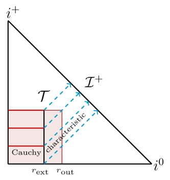
Figure 1: The conformal diagram of part of Minkowski spacetime, where spatial $i^{0}$, future temporal $i^{+}$ and future null $\mathcal{I}^{+}$ infinities are shown. In gravitational waveform modeling, the detector is assumed to be at $\mathcal{I}^{+}$. As is common in this context, we abuse the terminology “Cauchy” to denote the IBVP for a domain foliated by spacelike hypersurfaces that do not extend to $i^{0}$, but are truncated to some radius $r_{*}$, with $r_{*}=r_{\textrm{out}}$ for CCE and $r_{*}=r_{\textrm{ext}}$ for CCM. By “characteristic” we refer to the CIBVP for GR. For Cauchy-characteristic extraction (CCE) and matching (CCM) information between the Cauchy and characteristic domains is communicated via the worldtube $\mathcal{T}$.

The use of present and improved future gravitational wave (GW) detectors such as the ground-based advanced LIGO and Virgo Aasi et al. (2015); Acernese et al. (2015), Kagra Akutsu et al. (2020), the Cosmic Explorer Dwyer et al. (2015), and the Einstein Telescope Maggiore et al. (2020), as well as the space-borne detectors like LISA Amaro-Seoane et al. (2017), Taiji Ruan et al. (2020), and TianQin Luo et al. (2016), is already deepening and will continue to deepen our understanding of gravity. To harness their power, gravitational waveforms of high fidelity are necessary for the parameter estimation process Foucart et al. (2022). These waveform models are used to compare against observational data, and thus to infer the underlying properties of the sources.

In the modeling process, a GW detector is typically assumed to lie infinitely far away from the source in an asymptotically flat spacetime. After emission, GWs propagate toward future null infinity at the speed of light where they can be detected. There are different methods to calculate the detected gravitational radiation; see Bishop and Rezzolla (2016) for a review. A widely used technique is the extrapolation of the Weyl scalar $\psi_{4}$ to null infinity, which, in suitable coordinates Duarte et al. (2022), can be used to predict the effects of GWs on a detector. For this method, the initial boundary value problem (IBVP) that results in the production of GWs is solved, in a bounded numerical domain with outer boundary $r_{\textrm{out}}$. The value of $\psi_{4}$ is then calculated on worldtubes of different radii, and consequently used to fit a polynomial expansion, which is finally taken to calculate $\psi_{4}$ at the limit $r\rightarrow\infty$. This approach however is susceptible to systematic extrapolation errors, which can be avoided using the Cauchy-characteristic extraction (CCE) method Bishop et al. (1996a, 1997a, 1997b); Zlochower et al. (2003); Gomez et al. (2007); Babiuc et al. (2009); Reisswig et al. (2009, 2010); Winicour (2012); Handmer and Szilagyi (2015); Barkett et al. (2020); Moxon et al. (2020); Iozzo et al. (2021a); Mitman et al. (2021); Iozzo et al. (2021b); Mitman et al. (2020); Foucart et al. (2021); Moxon et al. (2021). CCE, as illustrated in Fig. 1, allows one to calculate the gravitational radiation at future null infinity $\mathcal{I}^{+}$ directly. In CCE, information from the Cauchy domain is passed through a worldtube $\mathcal{T}$ to the characteristic one, and propagated to $\mathcal{I}^{+}$.

Since the evolution of the Cauchy and the characteristic setups are decoupled, this method can still be affected by errors related to artificial boundary conditions imposed on the outer boundary of the Cauchy domain. One way to control these errors is to enlarge the Cauchy domain, such that the artificial boundary conditions on $r_{\textrm{out}}$ do not affect the solution within a smaller part of the domain, specifically up to the worldtube $r_{\textrm{ext}}$. The characteristic setup is then used to extract the solution from $r_{\textrm{ext}}$ to $\mathcal{I}^{+}$. However, the initial data provided on the initial null hypersurface for the characteristic initial boundary value problem (CIBVP) very often are not compatible with the IBVP solution outside $r_{\textrm{ext}}$, so there is still a type of error that has not been removed Taylor et al. (2013).

A way to avoid this type of error as well is to evolve the Cauchy and the characteristic setups simultaneously, and allow information to flow via $\mathcal{T}$ both ways. This approach is often called Cauchy-characteristic matching (CCM) and can in principle provide gravitational waveforms of high fidelity Bishop et al. (1996b, 1998); Winicour (2012). Recently, there has been an important effort to improve and optimize characteristic codes that can perform CCE and CCM Moxon et al. (2020, 2021). However, novel results regarding the hyperbolicity of general relativity (GR) in the characteristic setup Giannakopoulos et al. (2020, 2022) pose pressing questions as to whether CCE and CCM as currently performed for GR can indeed deliver on their promise to produce highly accurate waveforms.

Within the framework of numerical relativity, the CIBVP for the Einstein field equations (EFE) is typically constructed using a Bondi-like coordinate system Bondi et al. (1962); Winicour (2012); Cao and He (2013). In CCE and CCM, the resulting Bondi-like CIBVP is combined with the IBVP with a strongly or symmetric hyperbolic formulation of GR, such as the generalized harmonic formulation Pretorius (2005); Lindblom et al. (2006, 2008). Characteristic codes for GR based on a Bondi-like formulation have been widely used in numerical simulations. For instance, the first long-term evolution of a single black hole by the Binary Black Hole Grand Challenge Alliance Gómez et al. (1998), was achieved in such a setup. Many more codes have solved a Bondi-like CIBVP providing, for instance studies of relativistic stars Papadopoulos and Font (1999); Siebel et al. (2002), and gravitational collapse Garfinkle (1995); Crespo et al. (2019); Gundlach et al. (2019); Siebel et al. (2003); Alcoforado et al. (2021); Santos-Olivan and Sopuerta (2016); Santos-Olivan (2017). This success has led to the belief that these Bondi-like CIBVPs are well posed.

A partial differential equation (PDE) problem is well posed if it has a unique solution that depends continuously on the given data in an appropriate norm. Let us for example consider the first order, linear, constant coefficient system with real-valued variables and coefficients

$$\partial_{t}\mathbf{u}=\mathbf{B}^{p}\partial_{p}\mathbf{u}+\mathbf{B}\mathbf{u}\,,$$ (1)

where $\mathbf{u}$ is the state vector, $\partial_{p}$ denote spatial derivatives, $\mathbf{B}^{p}$ are the principal matrices and the product $\mathbf{B}\mathbf{u}$ denotes source terms. This system is weakly hyperbolic (WH) if the principal symbol $\mathbf{P}^{s}\equiv\mathbf{B}^{p}\mathbf{s}_{p}$ has real eigenvalues for all unit spatial covectors $\mathbf{s}_{p}$, and is called strongly hyperbolic (SH) if furthermore $\mathbf{P}^{s}$ is uniformly diagonalizable for all $\mathbf{s}^{p}$. In addition, if all the principal matrices $\mathbf{B}^{p}$ can be brought simultaneously in a symmetric form, then the system is called symmetric hyperbolic (SYMH).

Let us now consider the initial value problem (IVP) for the above system. Continuous dependence of the solution $\mathbf{u}$ at all times $t$ on the initial data $f$ can be understood as being able to provide an estimate of the form

$$||\mathbf{u}(\cdot,t)||\leq Ke^{\alpha t}||f||\,,$$ (2)

with real constants $K\geq 1$ and $\alpha\in\mathbb{R}$, and $||\cdot||$ denoting a suitable norm. The degree of hyperbolicity of the PDE system determines well-posedness of the problem, with the IVP for SH systems being (strongly) well posed in the $L^{2}$ norm of the system. On the contrary, the IVP of a system that is only WH but not SH, is ill posed in the $L^{2}$ norm. However, under certain conditions it may be weakly well posed in a different norm that is not equivalent to $L^{2}$. More details on weak well-posedness can be found in Kreiss and Lorenz (1989); Sarbach and Tiglio (2012). The essential difference between strong and weak well-posedness is that the first, in contrast to the second, is maintained in the presence of lower order perturbations (such as source terms).

The hyperbolicity analysis of free evolution schemes used in numerical relativity can be performed by bringing them to the form (1), via linearization and the constant coefficient approach. In Giannakopoulos et al. (2020) such an analysis was presented for the Bondi-Sachs free evolution system. Existence and uniqueness of solutions to the Bondi-like CIBVP were shown in Frittelli and Lehner (1999); Gomez and Frittelli (2003). In Frittelli (2005), a specific subsystem of the full system was found symmetric hyperbolic, and consequently certain norm estimates were provided. However, the hyperbolicity analyses presented in Giannakopoulos et al. (2020, 2022) which consider the full PDE system (in the linear, constant coefficient approximation), show that it is only weakly hyperbolic. This result is in contrast to that of Frittelli (2005) and implies that a Bondi-like CIBVP is ill posed in $L^{2}$ (in the linear, constant coefficient approximation). It is therefore remarkable that several characteristic codes can perform long simulations and produce physically sensible results. This fact, in combination with the existence of symmetric hyperbolic formulations of GR that involve third order metric derivatives and use Bondi-like gauges Rácz (2014); Cabet et al. (2014); Hilditch et al. (2020); Ripley (2021), suggests that there may still be some norm that is not equivalent to $L^{2}$, which can be used to demonstrate well-posedness of the standard Bondi-like CI(B)VP with energy estimates. By standard here we mean that GR is formulated only via the EFE so that only up to second order metric derivatives are involved, rather than including the Bianchi identities as in Rácz (2014); Cabet et al. (2014); Hilditch et al. (2020); Ripley (2021). However, finding such a norm and showing even weak well-posedness for these second order Bondi-like CI(B)VPs is still an open question.

Here, we concern ourselves with the following question: what are the best error estimates we can obtain for CCE and CCM with present setups and how can we test them numerically? To address this question we focus on simple toy models that have a structure similar to that of GR in the gauges typically employed. More specifically, we employ a characteristic model that is WH in a similar way to free evolution Bondi-like schemes, whereas the Cauchy model is SYMH like for instance GR in harmonic gauge. For completeness and comparison, we also consider cases with SYMH CIBVPs and WH IBVPs. The WH system is such that its IVP is weakly well posed. The paper has the following structure. In Sec. II we introduce the models we use for our analysis and provide energy estimates for each one of them. We also discuss under which conditions we can obtain an energy estimate for CCE and CCM. In Sec. III we discuss the discretization of the models, and perform numerical experiments to address convergence of solutions to discrete approximations of the previously discussed norms. We summarize our findings in Sec. IV and present our conclusions in Sec. V. Table 1 contains the list of all the acronyms used throughout the text.

Acronyms
CCE: Cauchy-Characteristic Extraction
CIBVP: Characteristic Initial Boundary Value Problem
CIVP: Characteristic Initial Value Problem
CCM: Cauchy-Characteristic Matching
EFE: Einstein Field Equations
GR: General Relativity
GW: Gravitational Wave
IBVP: Initial Boundary Value Problem
IVP: Initial Value Problem
PDE: Partial Differential Equation
SH: Strongly Hyperbolic
SYMH: Symmetric Hyperbolic
WH: Weakly Hyperbolic

Table 1: List of acronyms used throughout the text.

II The models

In this section we construct toy models and provide energy estimates for their solutions. For simplicity, we focus on first order, linear, constant coefficient, homogeneous and real-valued PDEs. We study energy estimates both for SYMH and WH models for the IBVP and the CIBVP, as well as for their CCE and CCM. The structure of the WH models are motivated by popular Bondi-like formulations of GR, and follows the model used in Giannakopoulos et al. (2020). Working with SYMH and not just SH systems allows us to mimic the best case scenario in a current GR CCM implementation, matching between a SYMH and a WH system for the IBVP and CIBVP respectively. Furthermore, estimates including boundary terms are simpler to obtain for SYMH systems than for systems that are only SH. The estimates presented in the section form the basis of our numerical tests presented in Sec. III.

II.1 The IBVP

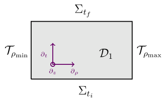
Figure 2: The Cauchy domain $\mathcal{D}_{1}$, with boundaries that are spacelike $\Sigma_{t_{i}}$, $\Sigma_{t_{f}}$ and timelike $\mathcal{T}_{\rho_{\textrm{min}}}$, $\mathcal{T}_{\rho_{\textrm{max}}}$. Initial data are provided on $\Sigma_{t_{i}}$ and boundary data on $\mathcal{T}_{\rho_{\textrm{min}}}$, $\mathcal{T}_{\rho_{\textrm{max}}}$ for the right- and left-moving variables, respectively. The $z$ direction is compact.

Our Cauchy PDE model system is

$$\partial_{t}\phi_{1} =-\partial_{\rho}\phi_{1}+\boxed{\partial_{z}\psi_{\varv 1}}\,,$$ (3a)

$$\partial_{t}\psi_{\varv 1} =-\partial_{\rho}\psi_{\varv 1}+\partial_{z}\phi_{1}\,,$$ (3b)

$$\partial_{t}\psi_{1} =\partial_{\rho}\psi_{1}+\partial_{z}\psi_{1}\,,$$ (3c)

with $\phi_{1},\psi_{\varv 1}$ the right-moving fields, and $\psi_{1}$ the left-moving. This system is SYMH when the boxed term of Eq. (3a) is included and only WH otherwise. The Cauchy domain $\mathcal{D}_{1}$ in which we seek a solution is formed by $t\in[t_{\textrm{i}},t_{\textrm{f}}]$, $\rho\in[\rho_{\textrm{min}},\rho_{\textrm{max}}]$, and $z\in[0,2\pi)$ with $z$ taken to be periodic; see Fig. 2 for an illustration. The given data for the IBVP consist of the initial and boundary data. The former are $\phi_{1}(t_{i},\rho,z)$, $\psi_{\varv 1}(t_{i},\rho,z)$, $\psi_{1}(t_{i},\rho,z)$ on an initial spacelike hypersurface $\Sigma_{t_{i}}$, while the latter are $\phi_{1}(t,\rho_{\textrm{min}},z)$, $\psi_{\varv 1}(t,\rho_{\textrm{min}},z)$ on the left boundary $\mathcal{T}_{\rho_{\textrm{min}}}$ since they are right moving, and $\psi_{1}(t,\rho_{\textrm{max}},z)$ on the right boundary $\mathcal{T}_{\rho_{\textrm{max}}}$, because it is left moving. The solution $\mathbf{u}_{1}$ to this IBVP at a later time $t_{f}>t_{i}$ consists then of $\phi_{1}(t_{f},\rho,z)$, $\psi_{\varv 1}(t_{f},\rho,z)$, $\psi_{1}(t_{f},\rho,z)$ on the final spacelike hypersurface $\Sigma_{t_{f}}$, as well as the values of the right-moving fields on the right boundary $\mathcal{T}_{\rho_{\textrm{max}}}$ and the left-moving on the left boundary $\mathcal{T}_{\rho_{\textrm{min}}}$ for all $t\in(t_{i},t_{f}]$.

To obtain an energy estimate for the solution to the IBVP of the SYMH system (3) we follow the standard procedure. Let us start with the $L^{2}$ norm

$$||\mathbf{u}_{1}||^{2}_{L^{2}(\Sigma_{t})}=\int\left(\phi_{1}^{2}+\psi_{\varv 1}^{2}+\psi_{1}^{2}\right)d\rho\,dz\,.$$ (4)

After acting on it with $\partial_{t}$, using the right-hand side (rhs) of Eq. (3) to replace $\partial_{t}\mathbf{u}_{1}$ and collecting total derivatives, we obtain

$$\partial_{t}||\mathbf{u}_{1}||^{2}_{L_{2}(\Sigma_{t})} =\int\left[-\partial_{\rho}\phi_{1}^{2}-\partial_{\rho}\psi_{\varv 1}^{2}+\partial_{\rho}\psi_{1}^{2}\right.$$

$$\left.\qquad\quad+2\partial_{z}\left(\phi_{1}\psi_{\varv 1}\right)+\partial_{z}\psi_{1}^{2}\right]d\rho\,dz\,,$$

where the total $\partial_{z}$ terms vanish since the data are assumed to be periodic in the $z$ direction throughout. Evaluating the total $\partial_{\rho}$ terms and integrating in $t\in[t_{i},t_{f}]$ we obtain

$$||\mathbf{u}_{1}||_{L^{2}(\Sigma_{t_{f}})}^{2}+\int_{\mathcal{T}_{\rho_{\textrm{max}}}}\left(\phi_{1}^{2}+\psi_{\varv 1}^{2}\right)+\int_{\mathcal{T}_{\rho_{\textrm{min}}}}\psi_{1}^{2}$$

$$=||\mathbf{u}_{1}||_{L^{2}(\Sigma_{t_{i}})}^{2}+\int_{\mathcal{T}_{\rho_{\textrm{min}}}}\left(\phi_{1}^{2}+\psi_{\varv 1}^{2}\right)+\int_{\mathcal{T}_{\rho_{\textrm{max}}}}\psi_{1}^{2}\,,$$ (5)

where we have rearranged terms such that the left-hand side (lhs) includes only the solution and the rhs only given data. This shows that the solution is completely controlled by the given data in the norm described by the lhs of Eq. (5).

Let us next consider the WH version of (3). First, let us note that we fail to obtain an energy estimate in the $L^{2}$ norm for the WH case, due to the boxed term in Eq. (3a). Instead, motivated by the analysis presented in Sec. III.B of Giannakopoulos et al. (2020), we start with the “lopsided” or $q$ norm

$$||\mathbf{u}_{1}||^{2}_{q(\Sigma_{t})}=\int\left[\phi_{1}^{2}+\psi_{\varv 1}^{2}+\psi_{1}^{2}+\left(\partial_{z}\phi_{1}\right)^{2}\right]d\rho\,dz\,,$$ (6)

where $q$ is due to the adoption of the notation of Kreiss and Lorenz (1989) for weak well-posedness and “lopsided” refers to the fact that only the angular derivative of a certain variable is included in the norm, and not of all variables. This norm leads to

$$\partial_{t}||\mathbf{u}_{1}||^{2}_{q(\Sigma_{t})} =\int\left[-\partial_{\rho}\phi_{1}^{2}-\partial_{\rho}\psi_{\varv 1}^{2}+\partial_{\rho}\psi_{1}^{2}-\partial_{\rho}\left(\partial_{z}\phi_{1}\right)^{2}\right.$$

$$\left.\qquad\quad+2\psi_{\varv 1}\partial_{z}\phi_{1}+\partial_{z}\psi_{1}^{2}\right]d\rho\,dz\,,$$

where now, due to the WH structure of the system the term $2\psi_{\varv 1}\partial_{z}\phi_{1}$ does not form a total derivative. The lopsided modification of the original $L^{2}$ norm was performed exactly in a way that allows us to control this term. To see this, let us first integrate in $t$ and drop the total derivative term $\partial_{z}\psi_{1}^{2}$ to obtain

$$||\mathbf{u}_{1}||_{q(\Sigma_{t_{f}})}^{2}=||\mathbf{u}_{1}||_{q(\Sigma_{t_{i}})}^{2}+\int_{\mathcal{T}_{\rho_{\textrm{min}}}}\left[\phi_{1}^{2}+\psi_{\varv 1}^{2}+\left(\partial_{z}\phi_{1}\right)^{2}-\psi_{1}^{2}\right]$$

$$\quad+\int_{\mathcal{T}_{\rho_{\textrm{max}}}}\psi_{1}^{2}-\phi_{1}^{2}-\psi_{\varv 1}^{2}-\left(\partial_{z}\phi_{1}\right)^{2}+\int_{\mathcal{D}_{1}}2\psi_{\varv 1}\partial_{z}\phi_{1}\,.$$

Using that $2\psi_{\varv 1}\partial_{z}\phi_{1}\leq\phi_{1}^{2}+\psi_{\varv 1}^{2}+\psi_{1}^{2}+\left(\partial_{z}\psi_{1}\right)^{2}$ the latter reads as

$$||\mathbf{u}_{1}||_{q(\Sigma_{t_{f}})}^{2}\leq||\mathbf{u}_{1}||_{q(\Sigma_{t_{i}})}^{2}+\int_{\mathcal{T}_{\rho_{\textrm{min}}}}\left[\phi_{1}^{2}+\psi_{\varv 1}^{2}+\left(\partial_{z}\phi_{1}\right)^{2}-\psi_{1}^{2}\right]$$

$$\quad+\int_{\mathcal{T}_{\rho_{\textrm{max}}}}\psi_{1}^{2}-\phi_{1}^{2}-\psi_{\varv 1}^{2}-\left(\partial_{z}\phi_{1}\right)^{2}+\int_{t_{i}}^{t_{f}}\int_{\Sigma_{t^{\prime}}}||\mathbf{u}_{1}||_{q(\Sigma_{t^{\prime}})}^{2}\,,$$

which after using Grönwall’s inequality yields

$$e^{t_{i}-t_{f}}||\mathbf{u}_{1}||_{q(\Sigma_{t_{f}})}^{2}+\int_{\mathcal{T}_{\rho_{\textrm{min}}}}\psi_{1}^{2}+\int_{\mathcal{T}_{\rho_{\textrm{max}}}}\left[\phi_{1}^{2}+\psi_{\varv 1}^{2}+\left(\partial_{z}\phi_{1}\right)^{2}\right]$$

$$\quad\leq||\mathbf{u}_{1}||_{q(\Sigma_{t_{i}})}^{2}+\int_{\mathcal{T}_{\rho_{\textrm{min}}}}\left[\phi_{1}^{2}+\psi_{\varv 1}^{2}+\left(\partial_{z}\phi_{1}\right)^{2}\right]+\int_{\mathcal{T}_{\rho_{\textrm{max}}}}\psi_{1}^{2}\,,$$ (7)

where we have rearranged terms such that the lhs includes only the solution, and the rhs only the given data, showing that the solution is completely controlled by the given data in the $q$ norm (6). It is important to remember that this result is subject to the structure of the source terms, and that for generic source terms one cannot provide such an energy estimate. This is the essential difference between strong and weak well-posedness.

Since the $q$ norm involves a specific derivative in its integrand, we find it useful to employ a norm for which one can show energy estimates for the SYMH IBVP, which also contains derivatives. We denote by $H_{1}$ the following norm:

$$||\mathbf{u}_{1}||^{2}_{H_{1}(\Sigma_{t})} =\int\left[\phi_{1}^{2}+\psi_{\varv 1}^{2}+\psi_{1}^{2}\right.$$

$$\left.+\left(\partial_{\rho}\phi_{1}\right)^{2}+\left(\partial_{\rho}\psi_{\varv 1}\right)^{2}+\left(\partial_{\rho}\psi_{1}\right)^{2}\right.$$

$$\left.+\left(\partial_{z}\phi_{1}\right)^{2}+\left(\partial_{z}\psi_{\varv 1}\right)^{2}+\left(\partial_{z}\psi_{1}\right)^{2}\right]d\rho\,dz\,.$$ (8)

Let us consider the first order system that is formed after we enlarge the SYMH system (3), by including $\partial_{\rho}\mathbf{u}_{1}$ and $\partial_{z}\mathbf{u}_{1}$ as variables. This system has the same principal structure as the original SYMH (3), and an energy estimate for its IBVP can be obtained starting with the $H_{1}$ norm (8). Following the same steps that led to the estimate (5) in the $L^{2}$ norm, one can show that

$$||\mathbf{u}_{1}||_{H_{1}(\Sigma_{t_{f}})}^{2}+\int_{\mathcal{T}_{\rho_{\textrm{min}}}}\left[\psi_{1}^{2}+\left(\partial_{\rho}\psi_{1}\right)^{2}+\left(\partial_{z}\psi_{1}\right)^{2}\right]$$

$$+\int_{\mathcal{T}_{\rho_{\textrm{max}}}}\left[\phi_{1}^{2}+\psi_{\varv 1}^{2}+\left(\partial_{\rho}\phi_{1}\right)^{2}+\left(\partial_{\rho}\psi_{\varv 1}\right)^{2}\right.$$

$$\qquad\qquad\left.+\left(\partial_{z}\phi_{1}\right)^{2}+\left(\partial_{z}\psi_{\varv 1}\right)^{2}\right]$$

$$=||\mathbf{u}_{1}||_{H_{1}(\Sigma_{t_{i}})}^{2}+\int_{\mathcal{T}_{\rho_{\textrm{max}}}}\left[\psi_{1}^{2}+\left(\partial_{\rho}\psi_{1}\right)^{2}+\left(\partial_{z}\psi_{1}\right)^{2}\right]$$

$$+\int_{\mathcal{T}_{\rho_{\textrm{min}}}}\left[\phi_{1}^{2}+\psi_{\varv 1}^{2}+\left(\partial_{\rho}\phi_{1}\right)^{2}+\left(\partial_{\rho}\psi_{\varv 1}\right)^{2}\right.$$

$$\qquad\qquad\left.+\left(\partial_{z}\phi_{1}\right)^{2}+\left(\partial_{z}\psi_{\varv 1}\right)^{2}\right]\,,$$ (9)

where again the lhs involves only the solution, and the rhs the given data. We can use this result to assess the well-posedness of the IBVP of the SYMH system (3), in a norm that includes derivatives. Notice that in comparison to the q norm (7), the $H_{1}$ norm (9) contains the same derivatives on all variables and so is symmetric, rather than lopsided.

II.2 The CIBVP

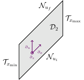
Figure 3: The characteristic domain $\mathcal{D}_{2}$, with boundaries that are null $\mathcal{N}_{u_{i}}$, $\mathcal{N}_{u_{f}}$ and timelike $\mathcal{T}_{x_{\textrm{min}}}$, $\mathcal{T}_{x_{\textrm{max}}}$. Initial data for left-moving fields are provided on $\mathcal{N}_{u_{i}}$ and boundary data on $\mathcal{T}_{\rho_{\textrm{min}}}$, $\mathcal{T}_{\rho_{\textrm{max}}}$ for the right- and left-moving variables, respectively. The $z$ direction is compact.

The characteristic model we consider is

$$\partial_{x}\phi_{2} =\boxed{\partial_{z}\psi_{\varv 2}}\,,$$ (10a)

$$\partial_{x}\psi_{\varv 2} =\partial_{z}\phi_{2}\,,$$ (10b)

$$\partial_{u}\psi_{2} =\frac{1}{2}\partial_{x}\psi_{2}+\partial_{z}\psi_{2}\,,$$ (10c)

where the fields $\phi_{2},\psi_{\varv 2}$ are right moving, and propagate with speed unity and $\psi_{2}$ is left moving with speed $1/2$. The system has two equations with derivatives only intrinsic to the characteristic surfaces $\mathcal{N}_{u}$ and one that includes also a derivative transverse to them. The system is SYMH when the boxed term in Eq. (10a) is included, and only WH otherwise. If we consider the coordinate transformation

$$u=t-\rho\,,\quad x=\rho\,,$$

which implies

$$\partial_{u}=\partial_{t}\,,\quad\partial_{x}=\partial_{t}+\partial_{\rho}\,,$$

the SYMH version of the system (10) is the characteristic version of the Cauchy system (3), provided that

$$\phi_{1} =\phi_{2}\,,\quad\psi_{\varv 1}=\psi_{\varv 2}\,\quad\psi_{1}=\psi_{2}\,,$$

and similarly for the WH one.

We consider the CIBVP for the characteristic domain $\mathcal{D}_{2}$ shown in Fig. 3, that consists of $u\in[u_{\textrm{i}},u_{\textrm{f}}]$, $x\in[x_{\textrm{min}},x_{\textrm{max}}]$, and $z\in[0,2\pi)$ with $z$ a periodic direction. The given data are the left-moving field $\psi_{2}(u_{i},x,z)$ on an initial characteristic $\mathcal{N}_{u_{i}}$, its value $\psi_{2}(u,x_{\textrm{max}},z)$ on the right boundary $\mathcal{T}_{x_{\textrm{max}}}$ and the values of the right-moving fields $\phi_{2}(u,x_{\textrm{min}},z)$, $\psi_{\varv 2}(u,x_{\textrm{min}},z)$ on the left boundary $\mathcal{T}_{x_{\textrm{min}}}$. The solution for which we next provide energy estimates consists of $\phi_{2}(u_{f},x,z)$ on a surface $\mathcal{N}_{u_{f}}$ with $u_{f}>u_{i}$, $\phi_{2}(u,x_{\textrm{min}},z)$ on the left boundary $\mathcal{T}_{x_{\textrm{min}}}$ and $\phi_{2}(u,x_{\textrm{max}},z)$, $\psi_{\varv 2}(u,x_{\textrm{max}},z)$ on the right boundary $\mathcal{T}_{x_{\textrm{max}}}$.

To obtain energy estimates in the characteristic domain, we can treat independently the left- and right-moving fields, due to the fact that the right-moving fields do not have an explicit $\partial_{u}$ time derivative. Let us first consider the left-moving field and start from the energy

$$||\mathbf{u}_{2}||^{2}_{\textrm{left}({\mathcal{N}_{u}})}=\int_{\mathcal{N}_{u}}\psi_{2}^{2}\,.$$

After acting with $\partial_{u}$ and replacing with the rhs of Eq. (10c) we obtain

$$\partial_{u}||\mathbf{u}_{2}||^{2}_{\textrm{left}({\mathcal{N}_{u}})}=\int_{\mathcal{N}_{u}}\partial_{x}\psi_{2}^{2}+\partial_{z}\psi_{2}^{2}\,.$$

By evaluating the total derivatives and integrating in $u\in[u_{i},u_{f}]$ we arrive at

$$2||\mathbf{u}_{2}||^{2}_{\textrm{left}({\mathcal{N}_{u_{f}}})}+\int_{\mathcal{T}_{x_{\textrm{min}}}}\psi_{2}^{2}=2||\mathbf{u}_{2}||^{2}_{\textrm{left}({\mathcal{N}_{u_{i}}})}+\int_{\mathcal{T}_{x_{\textrm{max}}}}\psi_{2}^{2}\,,$$ (11)

where we have rearranged terms such that the lhs contains only the solution and the rhs the given data, as well as multiplied everything by a factor of 2, to cancel the characteristic speed in the worldtube integrals. This estimate allows us to completely control the solution for the left-moving data by given data. If there are source terms in Eq. (10c) that include the right-moving fields, then the above calculation does not work. In that case one needs to perform the calculation for the whole system at once. Potentially, one also needs to consider a slightly different computational domain such that there is an integrand involving both left- and right-moving variables and offer the chance to control them using Grönwall’s inequality, as before. This however is beyond the scope of the current paper.

Next, we consider the right-moving fields, focusing first on the SYMH case. Let us start by considering the energy

$$||\mathbf{u}_{2}||^{2}_{\textrm{right}({\mathcal{T}_{x}})}=\int_{\mathcal{T}_{x}}\phi_{2}^{2}+\psi_{\varv 2}^{2}\,.$$

By acting with $\partial_{x}$ and replacing with the rhs of Eq. (10a), (10b) we obtain

$$\partial_{x}||\mathbf{u}_{2}||^{2}_{\textrm{right}({\mathcal{T}_{x}})}=\int_{\mathcal{T}_{x}}2\partial_{z}\left(\phi_{2}\psi_{\varv_{2}}\right)\,,$$

where the integrand on the right is a total $\partial_{z}$ term, and hence vanishes by periodicity in $z$. Then, integrating in $x\in[x_{\textrm{min}},x^{\prime}]$ for some $x^{\prime}\in(x_{\textrm{min}},x_{\textrm{max}}]$, we arrive at the estimate

$$||\mathbf{u}_{2}||^{2}_{\textrm{right}({\mathcal{T}_{x^{\prime}}})}=||\mathbf{u}_{2}||^{2}_{\textrm{right}({\mathcal{T}_{x_{\textrm{min}}}})}\,,$$ (12)

where the lhs is the solution and the rhs the given data. As was also done in a similar calculation in Giannakopoulos et al. (2020), we can take the supremum of $||\mathbf{u}_{2}||^{2}_{\textrm{right}({\mathcal{T}_{x^{\prime}}})}$ within $(x_{\textrm{min}},x_{\textrm{max}}]$ to obtain a better estimate, since $||\mathbf{u}_{2}||^{2}_{\textrm{right}({\mathcal{T}_{x^{\prime}}})}$ is not necessarily monotonically increasing with increasing $x^{\prime}$. Then, since Eq. (12) is true for all $x^{\prime}\in(x_{\textrm{min}},x_{\textrm{max}}]$ we obtain

$$\textrm{sup}_{x^{\prime}}||\mathbf{u}_{2}||^{2}_{\textrm{right}({\mathcal{T}_{x^{\prime}}})}=||\mathbf{u}_{2}||^{2}_{\textrm{right}({\mathcal{T}_{x_{\textrm{min}}}})}\,.$$ (13)

If we consider the WH model (10), then we should consider the energy

$$||\mathbf{u}_{2}||^{2}_{q-\textrm{right}({\mathcal{T}_{x}})}=\int_{\mathcal{T}_{x}}\phi_{2}^{2}+\psi_{\varv 2}^{2}+\left(\partial_{z}\phi_{2}\right)^{2}\,,$$

in analogy to the $q$ norm (6). Following the same steps as before we can arrive at

$$||\mathbf{u}_{2}||^{2}_{q-\textrm{right}({\mathcal{T}_{x^{\prime}}})}\leq||\mathbf{u}_{2}||^{2}_{q-\textrm{right}({\mathcal{T}_{x_{\textrm{min}}}})}+$$

$$\int_{x_{i}}^{x_{f}}||\mathbf{u}_{2}||^{2}_{q-\textrm{right}({\mathcal{T}_{x}})}dx\,,$$

where we have also used that $2\psi_{\varv 2}\partial_{z}\phi_{2}\leq\phi_{2}^{2}+\psi_{\varv 2}^{2}+\left(\partial_{z}\phi_{2}\right)^{2}$. Using again the Grönwall inequality and noticing that $||\mathbf{u}_{2}||^{2}_{q-\textrm{right}({\mathcal{T}_{x_{\textrm{min}}}})}$ involves only given (boundary) data, and hence is a constant function of $x$ or $x_{f}$ (so nondecreasing), we obtain

$$e^{x_{i}-x_{f}}\textrm{sup}_{x^{\prime}}||\mathbf{u}_{2}||^{2}_{q-\textrm{right}({\mathcal{T}_{x^{\prime}}})}\leq||\mathbf{u}_{2}||^{2}_{q-\textrm{right}({\mathcal{T}_{x_{\textrm{min}}}})}\,,$$ (14)

where we again took the supremum of $x^{\prime}$ to obtain a better estimate and the lhs contains only the solution and the rhs the given data and multiplied overall with $e^{x_{i}-x_{f}}$ for later convenience in the continuum analysis.

We can then proceed to add the estimates (11) and (12) to obtain the estimate for the homogeneous, symmetric hyperbolic system (10)

$$2||\mathbf{u}_{2}||^{2}_{\textrm{left}({\mathcal{N}_{u_{f}}})}+\textrm{sup}_{x^{\prime}}||\mathbf{u}_{2}||^{2}_{\textrm{right}({\mathcal{T}_{x^{\prime}}})}+\int_{\mathcal{T}_{x_{\textrm{min}}}}\psi_{2}^{2}=$$

$$2||\mathbf{u}_{2}||^{2}_{\textrm{left}({\mathcal{N}_{u_{i}}})}+||\mathbf{u}_{2}||^{2}_{\textrm{right}({\mathcal{T}_{x_{\textrm{min}}}})}+\int_{\mathcal{T}_{x_{\textrm{max}}}}\psi_{2}^{2}\,,$$ (15)

or add (11) and (14) to obtain an estimate for the WH characteristic model

$$2||\mathbf{u}_{2}||^{2}_{\textrm{left}({\mathcal{N}_{u_{f}}})}+e^{x_{i}-x_{f}}\textrm{sup}_{x^{\prime}}||\mathbf{u}_{2}||^{2}_{q-\textrm{right}({\mathcal{T}_{x^{\prime}}})}+\int_{\mathcal{T}_{x_{\textrm{min}}}}\psi_{2}^{2}$$

$$\leq 2||\mathbf{u}_{2}||^{2}_{\textrm{left}({\mathcal{N}_{u_{i}}})}+||\mathbf{u}_{2}||^{2}_{q-\textrm{right}({\mathcal{T}_{x_{\textrm{min}}}})}+\int_{\mathcal{T}_{x_{\textrm{max}}}}\psi_{2}^{2}\,.$$ (16)

Subsequently, we drop the factor of 2 in the lhs of Eq. (15) and (16) for convenience, but we still maintain the hypersurface integrals which provide the control of the solution on that region.

In analogy to the $H_{1}$ norm (8) for the SYMH IBVP, we also consider estimates in an $H_{1}$ norm adapted to the CIBVP, again by enlarging the SYMH characteristic system (10) with $\partial_{x}\mathbf{u}_{2}$ and $\partial_{z}\mathbf{u}_{2}$. In the characteristic $H_{1}$ norm one can show the following estimate for the enlarged system

$$2||\mathbf{u}_{2}||^{2}_{H_{1}-\textrm{left}({\mathcal{N}_{u_{f}}})}+\textrm{sup}_{x^{\prime}}||\mathbf{u}_{2}||^{2}_{H_{1}-\textrm{right}({\mathcal{T}_{x^{\prime}}})}+$$

$$\qquad\int_{\mathcal{T}_{x_{\textrm{min}}}}\left[\psi_{2}^{2}+\left(\partial_{x}\psi_{2}\right)^{2}+\left(\partial_{z}\psi_{2}\right)^{2}\right]$$

$$=2||\mathbf{u}_{2}||^{2}_{H_{1}-\textrm{left}({\mathcal{N}_{u_{i}}})}+||\mathbf{u}_{2}||^{2}_{H_{1}-\textrm{right}({\mathcal{T}_{x_{\textrm{min}}}})}+$$

$$\qquad\int_{\mathcal{T}_{x_{\textrm{max}}}}\left[\psi_{2}^{2}+\left(\partial_{x}\psi_{2}\right)^{2}+\left(\partial_{z}\psi_{2}\right)^{2}\right]\,,$$ (17)

with

$$||\mathbf{u}_{2}||^{2}_{H_{1}-\textrm{left}({\mathcal{N}_{u}})}=\int_{\mathcal{N}_{u}}\left[\psi_{2}^{2}+\left(\partial_{x}\psi_{2}\right)^{2}+\left(\partial_{z}\psi_{2}\right)^{2}\right]\,,$$

and

$$||\mathbf{u}_{2}||^{2}_{H_{1}-\textrm{right}({\mathcal{T}_{x}})}=\int_{\mathcal{T}_{x}}\left[\phi_{2}^{2}+\psi_{\varv 2}^{2}+\right.$$

$$\qquad\left.\left(\partial_{x}\phi_{2}\right)^{2}+\left(\partial_{x}\psi_{\varv 2}\right)^{2}+\left(\partial_{z}\phi_{2}\right)^{2}+\left(\partial_{z}\psi_{\varv 2}\right)^{2}\right]\,,$$

by simple commutation of partial derivatives.

II.3 CCE and CCM

Using the energy estimates from the previous subsections, we can now discuss energy estimates for CCE and CCM. For CCE the estimate follows straightforwardly from the previous results, and if both the IBVP and CIBVP are individually well posed in some norm, then CCE is too. The only detail that needs attention for this conclusion to be drawn is to choose the boundary data on $\mathcal{T}_{0}$ such that they are controlled in the appropriate norm for a WH CIBVP. Since these data are solutions of the IBVP, this may amount to having enough control over the derivatives of the solution on $\mathcal{T}_{0}$, so as to be controlled not only in the $L^{2}$ but also in the $H_{1}$ norm, as for instance shown in estimate (9). However, in this case we “lose” derivatives, in the sense that we control derivatives of more variables for the boundary data than for the solution to the WH CIBVP.

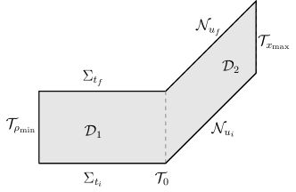
Figure 4: The CCM domain $\mathcal{D}_{3}=\mathcal{D}_{1}+\mathcal{D}_{2}$, with boundaries the spacelike $\Sigma_{t_{i}}$, $\Sigma_{t_{f}}$, the null $\mathcal{N}_{u_{i}}$, $\mathcal{N}_{u_{f}}$ and the timelike $\mathcal{T}_{\rho_{\textrm{min}}}$, $\mathcal{T}_{x_{\textrm{max}}}$. Initial data for all fields are provided on $\Sigma_{t_{i}}$, as well as on $\mathcal{N}_{u_{i}}$ only for left-moving fields. Boundary data are given on $\mathcal{T}_{\rho_{\textrm{min}}}$ for right-moving, and on $\mathcal{T}_{x_{\textrm{max}}}$ for left-moving fields. Data are communicated between the domains $\mathcal{D}_{1}$ and $\mathcal{D}_{2}$ via the worldtube $\mathcal{T}_{0}=\mathcal{T}_{\rho_{\textrm{max}}}=\mathcal{T}_{x_{\textrm{min}}}$. The $z$ direction is compact.

For the composite CCM problem to be well posed the situation is more complicated, as the norms in which the IBVP and the CIBVP are well posed need to be in some sense compatible. As shown in Giannakopoulos et al. (2020) the reason is that otherwise, there is a remaining integral over the interface $\mathcal{T}_{0}$ as shown in Fig. 4. For completeness, we briefly repeat here this calculation. First we consider matching the two SYMH setups. By adding the estimates (5) and (15) and using that $\mathbf{u}_{1}|_{\mathcal{T}_{0}}=\mathbf{u}_{2}|_{\mathcal{T}_{0}}$, we obtain

$$||\mathbf{u}_{1}||_{L_{2}(\Sigma(t_{f})}^{2}+||\mathbf{u}_{2}||^{2}_{\textrm{left}({\mathcal{N}_{u_{f}}})}$$ (18)

$$\qquad+\int_{\mathcal{T}_{\rho_{\textrm{min}}}}\psi_{1}^{2}+\textrm{sup}_{x^{\prime}}\int_{\mathcal{T}_{x^{\prime}}}\phi_{2}^{2}+\psi_{\varv 2}^{2}=$$

$$||\mathbf{u}_{1}||_{L_{2}(\Sigma(t_{i})}^{2}+||\mathbf{u}_{2}||^{2}_{\textrm{left}({\mathcal{N}_{u_{i}}})}+\int_{\mathcal{T}_{\rho_{\textrm{min}}}}\phi_{1}^{2}+\psi_{\varv 1}^{2}+\int_{\mathcal{T}_{x_{\textrm{max}}}}\psi_{2}^{2}\,.$$

The latter is the energy estimate for the composite CCM problem when matching the IBVP and CIBVP of the homogeneous symmetric hyperbolic Cauchy and characteristic systems (3) and (10), respectively. Notice that, as expected for the composite CCM problem, there is no worldtube integral over $\mathcal{T}_{0}$. A similar estimate can be obtained using the $H_{1}$ norms and adding the higher derivative estimates (9) and (17) for the SYMH IBVP and CIBVP, respectively.

Let us next consider matching the IBVP of the SYMH Cauchy system (3) to the weakly well-posed CIBVP of the WH characteristic system (10). In this case we add the energy estimates (5) and (16), which yields

$$||\mathbf{u}_{1}||_{L_{2}(\Sigma(t_{f})}^{2}+||\mathbf{u}_{2}||^{2}_{\textrm{left}({\mathcal{N}_{u_{f}}})}+$$

$$\int_{\mathcal{T}_{\rho_{\textrm{min}}}}\psi_{1}^{2}+e^{x_{i}-x_{f}}\textrm{sup}_{x^{\prime}}\int_{\mathcal{T}_{x^{\prime}}}\left[\phi_{2}^{2}+\psi_{\varv 2}^{2}+\left(\partial_{z}\phi_{2}\right)^{2}\right]$$

$$\leq||\mathbf{u}_{1}||_{L_{2}(\Sigma(t_{i})}^{2}+||\mathbf{u}_{2}||^{2}_{\textrm{left}({\mathcal{N}_{u_{i}}})}+$$

$$\int_{\mathcal{T}_{x_{\textrm{max}}}}\psi_{2}^{2}+\int_{\mathcal{T}_{\rho_{\textrm{min}}}}\left(\phi_{1}^{2}+\psi_{\varv 1}^{2}\right)+$$

$$\boxed{\int_{\mathcal{T}_{0}}\left(\partial_{z}\phi\right)^{2}}\,,$$ (19)

where we have used that on $\mathcal{T}_{0}$, $\mathbf{u}_{1}=\mathbf{u}_{2}$ in our models. The boxed term in the rhs of the latter is what prevents us from obtaining an energy estimate for the composite CCM in this setup and appears purely due to the incompatibility of the norms in which the IBVP and the CIBVP are well posed and weakly well posed, respectively. Since this term is not part of the given data, then the solution is not completely controlled by the intial and boundary data, and so the above is not a valid energy estimate for this composite CCM. If instead of using the $L^{2}$ estimate (5) for the IBVP, we use the $H_{1}$ estimate (9), the result would be similar, in that nonvanishing terms including an integral over the interface $\mathcal{T}_{0}$ remain.

Finally, we consider the matching of two WH setups. In this case, we combine the $q$ norm estimates (7) and (16) for the IBVP and CIBVP, respectively, to obtain

$$e^{t_{i}-t_{f}}||\mathbf{u}_{1}||_{q(\Sigma(t_{f})}+||\mathbf{u}_{2}||^{2}_{\textrm{left}({\mathcal{N}_{u_{f}}})}+$$

$$\int_{\mathcal{T}_{\rho_{\textrm{min}}}}\psi_{1}^{2}+e^{x_{i}-x_{f}}\textrm{sup}_{x^{\prime}}\int_{\mathcal{T}_{x^{\prime}}}\left[\phi_{2}^{2}+\psi_{\varv 2}^{2}+\left(\partial_{z}\phi_{2}\right)^{2}\right]$$

$$\leq||\mathbf{u}_{1}||_{q(\Sigma(t_{i})}+||\mathbf{u}_{2}||^{2}_{\textrm{left}({\mathcal{N}_{u_{i}}})}+$$

$$\int_{\mathcal{T}_{x_{\textrm{max}}}}\psi_{2}^{2}+\int_{\mathcal{T}_{\rho_{\textrm{min}}}}\left(\phi_{1}^{2}+\psi_{\varv 1}^{2}\right)\,.$$ (20)

In this case we see that, due to the compatibility of the norms, the integral over $\mathcal{T}_{0}$ vanishes and the lhs that contains only the solution, is completely controlled by the rhs, that includes only given data.

III Numerical experiments

We present numerical convergence tests for the individual IBVP and CIBVP, as well as for CCE and CCM, using discrete versions of the models analyzed in Sec. II. We work with the homogeneous models, unless explicitly stated otherwise. The implementation was performed using the Julia programming language Bezanson, Jeff and Edelman, Alan and Karpinski, Stefan and Shah, Viral B (2017) with the following details:

1. The numerical domain is defined by

   $$t\in[0,t_{f}]\,,\quad u\in[0,u_{f}]\,,$$

   $$\rho\in[-1,0]\,,\quad x\in[0,1]\,,\quad z\in[0,2\pi)\,,$$

   where $u=t-\rho$, so for $\rho=0$, $t_{f}=u_{f}$. We denote the grid points for $x$ as $x_{i}$ with $i\in[1,\dots,N]$ and the grid spacing as $h_{x}\equiv x_{2}-x_{1}$, and so forth.

2. All the derivatives that appear on the rhs of the systems (3) and (10) are approximated by second order accurate finite difference operators. The derivative $\partial_{x}$ is approximated with a centered stencil $D_{x}f_{i}=(f_{i+1}-f_{i-1})/(2h_{x})$ for the internal points of the $x$ grid. The derivative on the first and last points is approximated with upwind stencils that match the truncation error of the centered one

   $$D_{x}f_{1} =\frac{-4f_{1}+7f_{2}-4f_{3}+f_{4}}{2h_{x}}\,,$$ (21)

   $$D_{x}f_{N} =\frac{4f_{N}-7f_{N-1}+4f_{N-2}-f_{N-3}}{2h_{x}}\,.$$

   The same operators are used to approximate $\partial_{\rho}$, with $h_{x}\rightarrow h_{\rho}$, whereas for $\partial_{z}$, the centered stencil is used for the first and last points as well, taking advantage of the periodicity in $z$.

3. All fields that involve explicit time derivatives, that is $\phi_{1}\,,\psi_{\varv 1}\,,\psi_{1}\,,\psi_{2}$, are integrated in time using the explicit fourth order Runge-Kutta integration scheme.

4. The fields $\phi_{2}\,,\psi_{\varv 2}$ that satisfy equations intrinsic to the outgoing null hypersurfaces are integrated for every timestep from $x=0$ to $x=1$ using the trapezoidal rule, which is second order accurate.

5. No Kreiss-Oliger artificial dissipation is applied.

6. We choose a fixed timestep $h_{t}=0.25h_{\rho}$.

7. The initial data are $\phi_{1}(0,\rho,z)\,,\psi_{\varv 1}(0,\rho,z)\,,\psi_{1}(0,\rho,z)$ on the initial spacelike hypersurface $\Sigma_{t=0}$, and $\psi_{2}(0,x,z)$ on the initial null hypersurface $\mathcal{N}_{u=0}$.

8. For the IBVP, the boundary data are $\phi_{1}(t,-1,z)\,,\psi_{\varv 1}(t,-1,z)$ on the worldtube $\mathcal{T}_{\rho=-1}$, and $\psi_{1}(t,0,z)$ on $\mathcal{T}_{\rho=0}$.

9. For the CIBVP, $\phi_{2}(t,0,z)$ and $\psi_{\varv 2}(t,0,z)$ are provided as boundary data on the worldtube $\mathcal{T}_{x=0}$, as well as  $\psi_{2}(u,1,z)$ on $\mathcal{T}_{x=1}$.

10. For CCE, boundary data for the IBVP are given also on $\mathcal{T}_{\rho=0}$ for the left-moving field $\phi_{1}$. The values of the right-moving fields $\phi_{1}\,,\psi_{\varv 1}$ are propagated from the Cauchy to the characteristic domain via $\mathcal{T}_{\rho=x=0}$, as in CCM.

11. For CCM, on the worldtube (interface) $\mathcal{T}_{\rho=x=0}$ the values of the right-moving fields are propagated from the Cauchy to the characteristic domain via $\phi_{2}(u,0,z)=\phi_{1}(t,0,z)$, $\psi_{\varv 2}(u,0,z)=\psi_{\varv 1}(t,0,z)$, and for the left-moving one from the characteristic to the Cauchy via $\phi_{1}(t,0,z)=\phi_{2}(u,0,z)$.

12. For the tests presented in the paper, all the numerical boundary data are provided with pure injection, that is if $g_{1}(t,z)$ is the value of the grid function $\phi_{1}$ for $\rho=-1$, then $\phi_{1}(t,-1,z)=g_{1}(t,z)$. We have also experimented with a different method for numerical boundary data, namely by providing the time derivative rather than the field itself. The results can be found in Giannakopoulos et al. (2023a) and are qualitatively the same.

The main focus of this work is to examine the consequence of (a lack of) continuous dependence at the continuum level, as in (2), under numerical approximation. Detecting lack of convergence for WH systems can be subtle Calabrese et al. (2002). Numerical convergence tests that include high frequency data are a good choice in order to achieve this Calabrese et al. (2006); Cao and Hilditch (2012); Giannakopoulos et al. (2020). Low frequency data are not ideal to detect the effect of weak hyperbolicity in numerical simulations, since the solution may exhibit frequency dependent exponential or polynomial growth, that may not be evident for small frequencies in finite simulation time. Thus, the loss of convergence for an ill-posed problem may not be evident if the given data are not properly chosen. We run robust stability tests, which use high frequency given data, and monitor the convergence of the obtained numerical solutions in the norms presented in Sec. II.

Since we use uniform grids, we choose the high frequency data to be random noise of a certain amplitude. The random noise is added on top of an exact solution to the PDE problems, which in our tests is zero. We call these exact convergence tests, since we know the exact solution to the PDE problem. To fix ideas, next we present explicitly only the field $\phi_{1}$, but the discussion is the same for all fields $\psi_{\varv 1},\psi_{1},\phi_{2},\psi_{\varv 2},\psi_{2}$. If we denote by $\phi_{1}$ the continuum solution and $\phi_{1h}$ the numerical at resolution $h$, and assume that the dominant error for our discretization is due to the second order finite difference operators, then we expect the following relation to be true:

$$\phi_{1}=\phi_{1h}+O(h^{2})\,.$$

Given $\phi_{1}=0$ in our setup, it follows that

$$\phi_{1h}=O(h^{2})\,.$$

We denote by $h_{c}$ and $h_{m}$ the coarse and medium resolutions for which we solve the same PDE problem, and construct the convergence factor

$$Q\equiv\frac{h_{c}^{2}}{h_{m}^{2}}\simeq\frac{||\phi_{1c}||_{h_{c}}}{||\phi_{1m}||_{h_{m}}}\,,$$

where $\simeq$ here denotes equality up to terms of order $O(h_{c})$. Notice that the above relation is true only when the exact solution vanishes. Generically, when this is not true, one needs to replace $\phi_{1c}\rightarrow\phi_{1}-\phi_{1c}$ in the expression, and similarly for the medium resolution. Every time we increase resolution, we halve the grid spacing (for instance $h_{m}=h_{c}/2$), and therefore the expected convergence factor is $Q=4$. We construct and monitor the following quantity during our simulations

$$C_{\textrm{exact}}\equiv\log_{2}\frac{||\mathbf{u}_{h_{c}}||_{h_{c}}}{||\mathbf{u}_{h_{m}}||_{h_{m}}}\,,$$ (22)

where $||\cdot||_{h}$ is the discrete approximation to the continuum norm $||\cdot||$. The forms of the state vector $\mathbf{u}_{h}$ and the norm $||\cdot||_{h}$ depend on the specific discretized PDE problem solved, and so are clarified in the following subsections. Given that $Q=4$, perfect second order convergence corresponds to $C_{\textrm{exact}}=2$ for our exact convergence tests.

Motivated by the notation of the inequality (2), let us denote as $f_{h}$ the numerical initial and boundary data, which we specify as random noise of amplitude $A_{h}$ centered around zero. It is important to choose this amplitude appropriately such that $C_{\textrm{exact}}=2$ for all given data. Since $f_{h}\sim A_{h}$, for a field that appears without any derivative in the norm under consideration, we find that when $A_{h_{m}}=A_{h_{c}}/4$,

$$C_{\textrm{exact}}=\log_{2}\frac{||f_{h_{c}}||_{h_{c}}}{||f_{h_{m}}||_{h_{m}}}\sim\log_{2}\frac{O(A_{h_{c}})}{O(A_{h_{m}})}=2\,.$$

If however the norm includes a derivative of the field, then due to the finite difference operators used the exact convergence rate behaves as

$$\frac{O(A_{h_{c}})/h_{c}}{O(A_{h_{m}})/h_{m}}\,,$$

which for our setup is equal to 2 when we choose $A_{h_{m}}=A_{h_{c}}/8$. Consequently, our recipe to obtain given data that have $C_{\textrm{exact}}=2$ is the following: every time we double resolution, we drop the noise amplitude of the given data by a factor of 4 for any field with no derivative in the considered norm, and 8 for any field with at least one derivative in the considered norm.

The PDE setup	$L^{2}-L^{2}$ test	$q-q$ test	$H_{1}-H_{1}$ test	$H_{1}-q$ test
IBVP: SYMH (Fig. 5)	$C_{\textrm{exact}}=2$ (pass)	$C_{\textrm{exact}}=1$ (fail)	$C_{\textrm{exact}}=2$ (pass)	$C_{\textrm{exact}}=2$ (fail)
IBVP: WH (Fig. 5)	$C_{\textrm{exact}}=1$ (fail)	$C_{\textrm{exact}}=2$ (pass)	$C_{\textrm{exact}}=1$ (fail)	$C_{\textrm{exact}}=2$ (fail)
CIBVP: SYMH (Fig. 6)	$C_{\textrm{exact}}=2$ (pass)	$C_{\textrm{exact}}=1$ (fail)	$C_{\textrm{exact}}=2$ (pass)	$C_{\textrm{exact}}=2$ (fail)
CIBVP: WH (Fig. 6)	$C_{\textrm{exact}}=1$ (fail)	$C_{\textrm{exact}}=2$ (pass)	$C_{\textrm{exact}}=1$ (fail)	$C_{\textrm{exact}}=2$ (fail)
CIBVP of CCE: SYMH-WH (Fig. 7)	$C_{\textrm{exact}}=1$ (fail)	$C_{\textrm{exact}}=1$ (fail)	$C_{\textrm{exact}}=1$ (fail)	$C_{\textrm{exact}}=2$ (pass)
CIBVP of CCE: inhom. SYMH-WH (Fig. 11)	no test	no test	no test	$C_{\textrm{exact}}=2$ (pass)
CCM: SYMH-SYMH (Fig. 8)	$C_{\textrm{exact}}=2$ (pass)	$C_{\textrm{exact}}=1$ (fail)	$C_{\textrm{exact}}=2$ (pass)	$C_{\textrm{exact}}=2$ (fail)
CCM: WH-WH (Fig. 8)	$C_{\textrm{exact}}=1$ (fail)	$C_{\textrm{exact}}=2$ (pass)	$C_{\textrm{exact}}=1$ (fail)	$C_{\textrm{exact}}=2$ (fail)
CCM: SYMH-WH (Fig. 9)	$C_{\textrm{exact}}=1$ (fail)	$C_{\textrm{exact}}=1$ (fail)	$C_{\textrm{exact}}=1$ (fail)	$C_{\textrm{exact}}=2$ (fail)
CCM: inhom. SYMH-SYMH (Fig. 11)	no test	no test	$C_{\textrm{exact}}=2$ (pass)	no test
CCM: inhom. WH-WH (Fig. 11)	no test	$C_{\textrm{exact}}=2$ briefly (fail)	no test	no test
CCM: inhom. SYMH-WH (Fig. 10)	no convergence (fail)	no convergence (fail)	no convergence (fail)	no convergence (fail)

Table 2: Summary of the convergence tests presented in Sec. III. The first column shows the PDE setups that we have tested. All the setups are homogeneous, unless stated otherwise (“inhom.” stands for “inhomogeneous”). The second, third and forth columns show convergence tests where the same norm is used for the given data and the solution, whereas the last column shows a test where the given data are controlled in a norm bigger than the one we use to check the convergence of the solution. A test is considered as pass when $C_{\textrm{exact}}=2$ for the solution in the same norm as the given data, and fail otherwise (see text). Given our working definitions of pass and fail, the $H_{1}-q$ test should always fail by construction. The only case when we consider  $C_{\textrm{exact}}=2$ a pass for this test is for the CIBVP part of a SYMH-WH CCE setup. In this case, the $H_{1}$ controlled given data for the SYMH IBVP provide a solution that feeds boundary data to the WH CIBVP with enough control over the appropriate derivative terms. All our numerical convergence results are in line with our expectations from theory.

We run tests with given data that exhibit $C_{\textrm{exact}}=2$ in the appropriate $L^{2}$, $q$, or $H_{1}$ norm for the setup under consideration, and monitor the $C_{\textrm{exact}}$ of the solution in its $L^{2}$, $q$, or $H_{1}$ norm. We consider the test as passed if the solution converges in the same norm as the given data, at the same order; that is its $C_{\textrm{exact}}$ tends to $2$ with increasing resolution. In any other case we consider the test as failed. In our numerical experiments we see three different ways in which a test can fail:

1. $C_{\textrm{exact}}$ of the solution tends to a value different from 2 with increasing resolution, in the same norm as the given data.

2. $C_{\textrm{exact}}$ of the solution tends to 2 with increasing resolution, but in a norm different than the given data.

3. $C_{\textrm{exact}}$ does not tend to any fixed value with increasing resolution.

The first and second failing scenarios can actually happen for the same solution, if we just monitor its convergence in a different norm.

One argument to support our working definition of a passed and failed test is the following. Consider inequality (2) at the semidiscrete level, for instance at resolution $h$, namely

$$||\mathbf{u}_{h}||_{h}\leq Ke^{\alpha t}||f_{h}||_{h}\,,$$

with $K,\alpha$ real constants and $K\geq 1$. For a passed test we have that

$$4\simeq\frac{||f_{h}||_{h}}{||f_{h/2}||_{h/2}}=\frac{||\mathbf{u}_{h}||_{h}}{||\mathbf{u}_{h/2}||_{h/2}}\,,$$

where $\simeq$ here denotes equality up to terms of order $O(h)$, and therefore

$$||\mathbf{u}_{h/2}||_{h/2}\leq Ke^{\alpha t}||f_{h/2}||_{h/2}\,.$$

If this exact convergence rate is maintained for higher resolution runs, then we can imagine taking the limit of infinite resolution and recovering inequality (2) at the continuum. If, in contrast, during the tests we see the first type of failure, so that

$$\frac{||\mathbf{u}_{h}||_{h}}{||\mathbf{u}_{h/2}||_{h/2}}\simeq c\neq 4\simeq\frac{||f_{h}||_{h}}{||f_{h/2}||_{h/2}}\,,$$

with $c$ some real positive constant, then after doubling the resolution $n$ times we obtain

$$||\mathbf{u}_{h/2^{n}}||_{h/2^{n}} \leq\left(\frac{4}{c}\right)^{n}Ke^{\alpha t}||f_{h/2^{n}}||_{h/2^{n}}$$

$$=\tilde{K}e^{\alpha t}||f_{h/2^{n}}||_{h/2^{n}}\,,$$

with $\tilde{K}\equiv\left(4/c\right)^{n}K$. If $c<4$ consistently, then in the limit of infinite resolution $n\rightarrow\infty$, $\tilde{K}\rightarrow\infty$, whereas if $c>4$ consistently, $\tilde{K}\rightarrow 0$ as $n\rightarrow\infty$. In either case one does not recover the continuum version of inequality (2), which we interpret as failure of the solution to be controlled by the given data. In this argument we consider the theoretically expected value of $C_{\textrm{exact}}$ for both the solution and the given data, but in practice, we look for a $C_{\textrm{exact}}$ that tends to that value.

The second type of failure is an interesting scenario realized in our tests, where we obtain the same convergence rate for the solution and the given data, but only in different norms,

$$4\simeq\frac{||f_{h}||_{H_{1}}}{||f_{h/2}||_{H_{1}}}=\frac{||\mathbf{u}_{h}||_{q}}{||\mathbf{u}_{h/2}||_{q}}\,,$$

where we have dropped the subscript $\sim h$ in the different discrete norms. In this case, one can at most obtain the following inequality:

$$||\mathbf{u}||_{q}\leq Ke^{\alpha t}||f||_{H_{1}}\,,$$ (23)

by considering again the limit of infinite resolution, This however is not the same as inequality (2), which is involved in the textbook definition of well-posedness. More importantly, since $||\mathbf{u}||_{q}$ is smaller than $||\mathbf{u}||_{H_{1}}$ (controls fewer derivative terms), it is perfectly possible to obtain a solution $\mathbf{u}$ with unbounded $H_{1}$, but bounded $q$ norm. In this case, the blowup would appear in derivatives of the solution that are included in $H_{1}$ but not in the $q$ norm. We therefore consider this scenario also a failure.

The lowest resolution we use for our tests is denoted by $h_{0}$ and has $N_{\rho}=N_{x}=17$ and $N_{z}=16$. The grid points and grid spacing for the different resolutions are set according to

$$N_{\rho}=N_{x}=16^{2D}+1\,,\quad N_{z}=16^{2D}\,,$$

$$h_{\rho}=h_{x}=\frac{1}{N_{\rho}-1}\,,\quad h_{z}=\frac{2\pi}{N_{z}}\,,$$

and $h_{D}$ labels the different resolutions, for instance $D=0$ corresponds to the lowest resolution $h_{0}$. We perform tests for $D=0,1,2,3,4$, and compute $C_{\textrm{exact}}$ only for the timesteps that are common across all resolutions, in other words at each timestep with $h_{0}$ grid spacing. The code and parameter files for the convergence tests can be found in Giannakopoulos et al. (2023a) and the data used to produce the following convergence plots in Giannakopoulos et al. (2023b). In the following subsections, all the norms should be understood as evaluated on the numerical grid. Table 2 contains the summary of our numerical experiments.

III.1 IBVP

First we examine numerical convergence of the Cauchy setup. The discrete norms in which we test the convergence of the solution are

$$||\mathbf{u}_{1}||^{2}_{L^{2}}=\sum_{\rho,z}\left(\phi_{1}^{2}+\psi_{\varv 1}^{2}+\psi_{1}^{2}\right)\,h_{\rho}h_{z}$$ (24)

$$\qquad\qquad+\sum_{t,\rho=-1,z}\psi_{1}^{2}\,h_{t}h_{z}+\sum_{t,\rho=0,z}\left(\phi_{1}^{2}+\psi_{\varv 1}^{2}\right)\,h_{t}h_{z}\,,$$

$$||\mathbf{u}_{1}||^{2}_{q}=\sum_{\rho,z}\left[\phi_{1}^{2}+\psi_{\varv 1}^{2}+\psi_{1}^{2}+\left(D_{z}\phi_{1}\right)^{2}\right]\,h_{\rho}h_{z}$$ (25)

$$+\sum_{t,\rho=-1,z}\psi_{1}^{2}\,h_{t}h_{z}+\sum_{t,\rho=0,z}\left[\phi_{1}^{2}+\psi_{\varv 1}^{2}+\left(D_{z}\phi_{1}\right)^{2}\right]\,h_{t}h_{z}\,,$$

$$||\mathbf{u}_{1}||^{2}_{H_{1}}=\sum_{\rho,z}\left[\phi_{1}^{2}+\psi_{\varv 1}^{2}+\psi_{1}^{2}\right.$$ (26)

$$\left.\qquad\qquad\qquad+\left(D_{\rho}\phi_{1}\right)^{2}+\left(D_{\rho}\psi_{\varv 1}\right)^{2}+\left(D_{\rho}\psi_{1}\right)^{2}\right.$$

$$\left.\qquad\qquad\qquad+\left(D_{z}\phi_{1}\right)^{2}+\left(D_{z}\psi_{\varv 1}\right)^{2}+\left(D_{z}\psi_{1}\right)^{2}\right]\,h_{\rho}h_{z}$$

$$\qquad+\sum_{t,\rho=-1,z}\left[\psi_{1}^{2}+\left(D_{\rho}\psi_{1}\right)^{2}+\left(D_{z}\psi_{1}\right)^{2}\right]\,h_{t}h_{z}$$

$$\quad+\sum_{t,\rho=0,z}\left[\phi_{1}^{2}+\psi_{\varv 1}^{2}+\left(D_{\rho}\phi_{1}\right)^{2}+\left(D_{\rho}\psi_{\varv 1}\right)^{2}\right.$$

$$\qquad\qquad\left.+\left(D_{z}\phi_{1}\right)^{2}+\left(D_{z}\psi_{\varv 1}\right)^{2}\right]\,h_{t}h_{z}\,.$$

In our tests, we choose given data that converge in either the $L^{2}$, $q$, or $H_{1}$ norms. Based on the energy estimates given Sec. II.1, these can be obtained by considering Eqs. (24)-(26), but where the spacelike hypersurface sums are evaluated only for the initial data, and the worldtube sums on the left boundary for right-moving fields and on the right boundary for left-moving fields, i.e., the opposite of what is shown. We perform four different tests:

1. $L^{2}-L^{2}$ test: convergence of the solution in the $L^{2}$ norm (24), for $L^{2}$ given data.

2. $q-q$ test: convergence of the solution in the $q$ norm (25), for $q$ given data.

3. $H_{1}-H_{1}$ test: convergence of the solution in the $H_{1}$ norm (26), for $H_{1}$ given data.

4. $H_{1}-q$ test: convergence of the solution in the $q$ norm (25), for $H_{1}$ given data.

The $L^{2}-L^{2}$, $q-q$, and $H_{1}-H_{1}$ tests examine, at the discrete level, continuous dependence of the solution on the given data as described by inequality (2). In contrast, the $H_{1}-q$ test examines the discrete version of inequality (23). If the latter is satisfied, it shows that a solution is controlled by given data that converge in a bigger norm. In our particular setup, the $q$ norm (25) is smaller than the $H_{1}$ (26) in the sense that it allows control over fewer derivative terms. It then becomes clear that a blowup in a derivative of the solution can still happen, but fail to be detected by the $q$ norm. We consider this test because it can explain why CCE involving a SYMH IBVP and a WH CIBVP can result in well-posed PDE problems that exhibit the expected numerical convergence. But the $H_{1}-q$ test does not address continuous dependence as understood in the standard sense for well-posedness as in inequality (2).

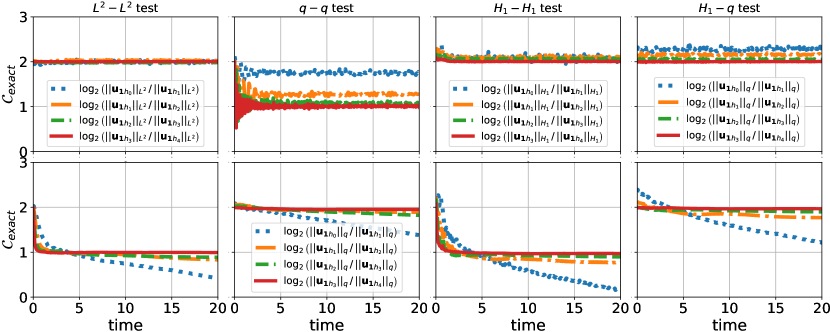
Figure 5: The exact convergence rate $\mathcal{C}_{\textrm{exact}}$ is shown for the IBVP, for all the tests. The top row refers to the SYMH setup, and the bottom to the WH one. The left column presents the results for the $L^{2}-L^{2}$ test, the second to left for the $q-q$ test, and so on. The results of the $L^{2}-L^{2}$, $q-q$, and $H_{1}-H_{1}$ tests are as expected by theory, that is convergence in the $L^{2}$ and $H_{1}$ for the SYMH case and in the $q$ norm for the WH one. The convergence in the $q$ norm seen in the $H_{1}-q$ test is merely a result of the fact that $H_{1}$ (26) is a bigger norm than $q$ (25), in the sense that it controls more derivative terms. We only monitor the $\partial_{z}\phi_{1}$ derivative term, which still converges appropriately for the SYMH case and due to its size in comparison to the nonderivate terms, dominates the $q$ norm. We also see good convergence of the solution to the WH IBVP in the $H_{1}-q$ test, because we ignore the derivative terms that do not exhibit convergence. The plots for the $H_{1}-H_{1}$ and $H_{1}-q$ tests use data from exactly the same runs.

The findings of our numerical tests are shown in Fig. 5. The top row of the figure shows $\mathcal{C}_{\textrm{exact}}$ for a SYMH IBVP setup, whereas the bottom is for a WH one. Each column refers to one test, starting from the left and moving to the right with the $L^{2}-L^{2}$, $q-q$, $H_{1}-H_{1}$, and finally the $H_{1}-q$ test. The first three provide the expected convergence results, that is, for the SYMH case, good empirical convergence of the solution in $L^{2}$ and $H_{1}$ norms and loss of convergence in the $q$ norm. In contrast in the WH case, we see $\mathcal{C}_{\textrm{exact}}=2$ only for the $q-q$ test. The $H_{1}-q$ test returns interesting and potentially confusing results: both solutions to the SYMH and WH setups exhibit good convergence in the $q$ norm for given data controlled in their $H_{1}$ norm. This can be understood in the following terms:

1. SYMH: by monitoring the $q$ norm, we take into account only the $\partial_{z}\phi_{1}$ derivative of the solution. This part still converges appropriately, and due to its relative size in comparison to the nonderivative terms, dominates the convergence rate. This does not mean that the $H_{1}-q$ test provides numerical evidence for well-posedness of the SYMH IBVP in the $q$ norm, which would be the case if the $q-q$ test was passed.

2. WH: when we monitor the $q$ norm, we ignore all the derivatives that appear in $H_{1}$ and not in $q$, which are responsible for the loss of convergence. We only monitor the $\partial_{z}\phi_{1}$ term, which converges properly and due to its relative size, dominates the nonderivative terms of the $q$ norm. Since we are considering the homogeneous case, the loss of convergence of the nonmonitored derivative terms does not propagate to $\partial_{z}\phi_{1}$ due to the lack of a coupling among them. Finally, proper convergence of the given data in the $H_{1}$ norm implies the same in the $q$ norm, since $H_{1}$ is bigger than $q$.

When we see loss of convergence in these tests we observe $C_{\textrm{exact}}=1$, and since this is not the expected rate of convergence for our numerical scheme, we consider these tests as failed. However, it is often the case in physically interesting simulations that the convergence order of the solution is lower than that of the numerical scheme used (for instance shockwave capturing or schemes that include interpolation). Here, we insist in considering these tests as failed, because we do not have additional elements in the scheme that can drop the order of convergence (the data are smooth plus the artificially exaggerated numerical error, no interpolations) and more importantly we try to make contact with the continuum energy estimates. As a final remark on this point, we should mention that it is not clear why $C_{\textrm{exact}}=1$ in these cases. A possibility is that it relates to the bulk integrals in the continuum analysis that prevent us from obtaining energy estimates for the scenarios of the failed tests. Obtaining however a concrete answer requires more testing and is beyond the scope of this work.

III.1.1 Synopsis

The SYMH IBVP exhibits second order convergence in the $L^{2}$ and $H_{1}$ norms for given data controlled in the same norms, and second order convergence in the $q$ norm only when the given data are controlled in the $H_{1}$ norm. The WH IBVP shows second order convergence in the $q$ norm for given data controlled in either their $q$ and $H_{1}$ norms. These results are inline with the expectations from theory.

III.2 CIBVP

We repeat the tests for the CIBVP, monitoring the convergence of the solution in the following discrete norms

$$||\mathbf{u}_{2}||^{2}_{L^{2}}=\sum_{x,z}\psi_{2}^{2}\,h_{x}h_{z}+\sum_{u,x=0,z}\psi_{2}^{2}\,h_{u}h_{z}$$ (27)

$$\qquad\qquad+\textrm{max}_{x}\sum_{u,z}\left(\phi_{2}^{2}+\psi_{\varv 2}^{2}\right)\,h_{u}h_{z}\,,$$

$$||\mathbf{u}_{2}||^{2}_{q}=\sum_{x,z}\psi_{2}^{2}\,h_{x}h_{z}+\sum_{u,x=0,z}\psi_{2}^{2}\,h_{u}h_{z}$$ (28)

$$\qquad\qquad+\textrm{max}_{x}\sum_{u,z}\left[\phi_{2}^{2}+\psi_{\varv 2}^{2}+\left(D_{z}\phi_{2}\right)^{2}\right]\,h_{u}h_{z}\,,$$

and

$$||\mathbf{u}_{2}||^{2}_{H_{1}}=\sum_{x,z}\left[\phi_{2}^{2}+\left(D_{x}\psi_{2}\right)^{2}+\left(D_{z}\psi_{2}\right)^{2}\right]\,h_{x}h_{z}$$ (29)

$$\qquad+\sum_{u,x=-0,z}\left[\psi_{2}^{2}+\left(D_{x}\psi_{2}\right)^{2}+\left(D_{z}\psi_{2}\right)^{2}\right]\,h_{u}h_{z}$$

$$\quad+\textrm{max}_{x}\sum_{u,z}\left[\phi_{2}^{2}+\psi_{\varv 2}^{2}+\left(D_{x}\phi_{2}\right)^{2}+\left(D_{x}\psi_{\varv 2}\right)^{2}\right.$$

$$\qquad\qquad\left.+\left(D_{z}\phi_{2}\right)^{2}+\left(D_{z}\psi_{\varv 2}\right)^{2}\right]\,h_{u}h_{z}\,.$$

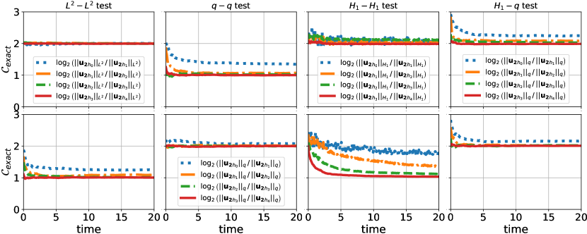
Figure 6: Exact convergence rate $\mathcal{C}_{\textrm{exact}}$ for the CIBVP solution, for our tests in the different norms. The SYMH setup is shown in top row and the WH one in the bottom. Each column shows the results of each test. The $L^{2}-L^{2}$, $q-q$, and $H_{1}-H_{1}$ tests exhibit the expected convergence in the $L^{2}$ and $H_{1}$ for SYMH and in the $q$ norm for WH. Convergence in the $q$ norm seen in the $H_{1}-q$ test is again a result of the fact that $H_{1}$ (29) is bigger than the $q$ (28) norm, as in the IBVP. The plots for the $H_{1}-H_{1}$ and $H_{1}-q$ tests use data from exactly the same runs.

III.2.1 Synopsis

The results are qualitatively the same as for the IBVP, and are summarized in Fig. 6. We again find the expected convergence rate in $L^{2}$ and $H_{1}$ for the SYMH and in the $q$ norm for the WH setup. The $H_{1}-q$ test provides apparent convergence in the $q$ norm for both setups, which is understood exactly in the same way as in the IBVP.

III.3 CCE

The conclusions drawn from the previous tests for the IBVP and CIBVP shape our expectations for CCE. In this setup, convergence of the numerical solution is still examined for the individual IBVP and CIBVP parts of the CCE scheme. The important difference now is that part of the IBVP solution serves as boundary data (for the right-moving fields) for the CIBVP. When performing these tests for CCE we expect the following results:

1. CCE between a SYMH IBVP and a SYMH CIBVP: both IBVP and CIBVP solutions converge in $L^{2}$ and $H_{1}$, but not in the $q$ norm. The $H_{1}-q$ test has the same qualitative results as in Secs. III.1 and III.2.

2. WH-WH CCE: Both IBVP and CIBVP converge only in the $q$ norm, but not in $L^{2}$ or $H_{1}$. The $H_{1}-q$ test shows again that both solutions converge in their $q$ norms for the $H_{1}$ given data.

3. SYMH-WH CCE: The solution to the IBVP exhibits the same behavior as in Sec. III.1. The solution to the CIBVP can converge properly only in the $q$ norm. The boundary data to the CIBVP are part of the solution to the IBVP and so we need a solution to the IBVP that converges properly in the $H_{1}$ norm, such that the boundary data to the CIBVP also converge properly in the $q$ norm (neglecting the derivatives that are in $H_{1}$ but not in $q$). The aforementioned setup is understood in the $H_{1}-q$ test. In addition, choosing characteristic initial data that converge in $L^{2}$ or $H_{1}$ does not affect the convergence of the CIBVP solution in the $q$ norm. The reason is that the derivative term $\partial_{z}\phi_{2}$ dominates the characteristic $q$ norm (28). For our tests we drop the amplitude of $\phi_{2}(u=0,x,z)$ by a factor of 8 every time the grid spacing is halved, that is compatible with $H_{1}$.

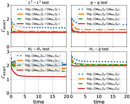
Figure 7: $\mathcal{C}_{\textrm{exact}}$ for all our tests, for the CIBVP part of a CCE setup between a SYMH IBVP and a WH CIBVP. As expected, only the $H_{1}-q$ test provides good convergence. In this case, the $H_{1}$ given data provide an $H_{1}$ controlled solution to the IBVP, part of which serves as boundary data for the WH CIBVP. That control is more than enough to have $q$ controlled given data for the CIBVP, and hence, the solution to the CIBVP is controlled in the $q$ norm.

Repeating these tests for CCE, our expectations were verified. The SYMH-WH scenario is the relevant one for current implementations of CCE in GR simulations, and therefore we present only these results in Fig. 7. We see that indeed the solution to the WH CIBVP setup exhibits the appropriate convergence rate only when $H_{1}$ data are given for the IBVP. The solution to that IBVP provides boundary data for the CIBVP that have $H_{1}$ control, which is more than the necessary control in the $q$ norm. This result is compatible with that of the $H_{1}-q$ test in Sec. III.2.

III.3.1 Synopsis

CCE between a SYMH IBVP and a weakly well-posed WH CIBVP, can only provide a characteristic solution with second order convergence in its $q$ norm, if the solution of the SYMH IBVP is controlled in its $H_{1}$ norm. This is inline with our expectations from theory.

III.4 CCM

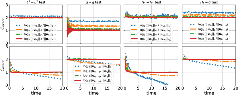
Figure 8: The exact convergence rate of the CCM solution, for SYMH-SYMH (top) and WH-WH (bottom). The first column refers to the $L^{2}-L^{2}$ test, the second to the $q-q$ test, and so on. The $L^{2}-L^{2}$, $q-q$, and $H_{1}-H_{1}$ tests show the expected convergence in the $L^{2}$ and $H_{1}$ for SYMH-SYMH and in the $q$ norm for WH-WH. The convergence in the $q$ norm seen in the $H_{1}-q$ test is again a result of the fact that $H_{1}$ (32) is bigger than $q$ (31), as in the IBVP. The plots for the $H_{1}-H_{1}$ and $H_{1}-q$ tests use data from exactly the same runs.

The discrete norms for which we run our tests for CCM are

$$||\mathbf{u}||^{2}_{L^{2}}=\sum_{\rho,z}\left(\phi_{1}^{2}+\psi_{\varv 1}^{2}+\psi_{1}^{2}\right)\,h_{\rho}h_{z}+\sum_{x,z}\psi_{2}^{2}\,h_{x}h_{z}$$

$$+\sum_{t,\rho=-1,z}\psi_{1}^{2}\,h_{t}h_{z}+\textrm{max}_{x}\sum_{u,x,z}\left(\phi_{2}^{2}+\psi_{\varv 2}^{2}\right)\,h_{u}h_{z}\,.$$ (30)

$$||\mathbf{u}||^{2}_{q}=\sum_{\rho,z}\left(\phi_{1}^{2}+\psi_{\varv 1}^{2}+\psi_{1}^{2}\right)\,h_{\rho}h_{z}+\sum_{x,z}\psi_{2}^{2}\,h_{x}h_{z}$$ (31)

$$+\sum_{t,\rho=-1,z}\psi_{1}^{2}\,h_{t}h_{z}+\textrm{max}_{x}\sum_{u,x,z}\left[\phi_{2}^{2}+\psi_{\varv 2}^{2}+\left(D_{z}\phi_{2}\right)^{2}\right]\,h_{u}h_{z}\,,$$

$$||\mathbf{u}||^{2}_{H_{1}}=\sum_{\rho,z}\left[\phi_{1}^{2}+\psi_{\varv 1}^{2}+\psi_{1}^{2}+\left(D_{\rho}\phi_{1}\right)^{2}+\left(D_{\rho}\psi_{\varv 1}\right)^{2}\right.$$

$$\left.+\left(D_{\rho}\psi_{1}\right)^{2}+\left(D_{z}\phi_{1}\right)^{2}+\left(D_{z}\psi_{\varv 1}\right)^{2}+\left(D_{z}\psi_{1}\right)^{2}\right]\,h_{\rho}h_{z}$$

$$+\sum_{x,z}\left[\psi_{2}^{2}+\left(D_{x}\psi_{2}\right)^{2}+\left(D_{z}\psi_{2}\right)^{2}\right]\,h_{x}h_{z}$$

$$+\sum_{t,\rho=-1,z}\left[\psi_{1}^{2}+\left(D_{\rho}\psi_{1}\right)^{2}+\left(D_{z}\psi_{1}\right)^{2}\right]\,h_{t}h_{z}$$

$$+\textrm{max}_{x}\sum_{u,x,z}\left[\phi_{2}^{2}+\psi_{\varv 2}^{2}+\left(D_{x}\phi_{2}\right)^{2}+\left(D_{x}\psi_{\varv 2}\right)^{2}\right.$$

$$\qquad\qquad\qquad\left.+\left(D_{z}\phi_{2}\right)^{2}+\left(D_{z}\psi_{\varv 2}\right)^{2}\right]\,h_{u}h_{z}\,.$$ (32)

First, let use consider matching PDEs with the same degree of hyperbolicity, that is SYMH to SYMH or WH to WH. The convergence results of these setups are shown in Fig. 8, with SYMH-SYMH at the top and WH-WH the bottom row. As expected by the energy estimates of Sec. II.3, we see good convergence for SYMH-SYMH in the $L^{2}-L^{2}$ and $H_{1}-H_{1}$ tests that is in norms $L^{2}$ (30) and $H_{1}$ (32) respectively, and in the $q-q$ test for the WH-WH case, i.e. norm $q$ (31). In the $H_{1}-q$ test we see convergence of the solution in the $q$ norm (31) for $H_{1}$ given data, in line with the results of the same test for the IBVP and CIBVP. The explanation of this phenomenon is the same as earlier, that is for the SYMH-SYMH setup we see the convergence of the $\partial_{z}\phi_{2}$ term that dominates the norm, whereas in the WH-WH setup we ignore the rest of the derivative terms that do not converge.

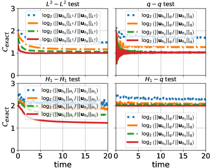
Figure 9: $\mathcal{C}_{\textrm{exact}}$ for a SYMH-WH CCM setup. The $L^{2}-L^{2}$ test is shown in top left, the $q-q$ in top right, the $H_{1}-H_{1}$ in bottom left, and the $H_{1}-q$ test in bottom right. The first three tests fail to exhibit the appropriate convergence rate, as expected for this setup. The $H_{1}-q$ test manifests convergence in the $q$ norm (31), again due to the fact that $H_{1}$ (32) is a bigger norm. The fact that the behavior seen is similar to that of the CIBVP part of CCE, in Fig. 7, is a result of treating the homogeneous case. In Fig. 10 we see that the behavior is different for an inhomogeneous SYMH-WH CCM setup.

Next we consider the matching of a SYMH IBVP to a WH CIBVP, the actual case for CCM in GR as currently performed. The convergence plots are presented in Fig. 9. We see that the solution does not exhibit good convergence in any norm for the $L^{2}-L^{2}$, $q-q$, and $H_{1}-H_{1}$ tests, which are the ones that reflect numerically continuous dependence on given data. Only the  $H_{1}-q$ test shows good convergence of the solution in the $q$ norm for $H_{1}$ given data. This test only provides numerical support for inequality (23) rather than (2). Comparing Fig. 7 with Fig. 9, we see the same qualitative behavior, namely good convergence only for the $H_{1}-q$ test. The latter refers to CCM and the former the CIBVP part of CCE, both for a SYMH IBVP and a WH CIBVP. The difference between CCM and CCE is only the additional propagation of information between the characteristic and Cauchy domain for the left-moving field for CCM. Since we are considering only the homogeneous case here, we see that there is no structure in the composite system that couples the right-moving variables of the characteristic domain that are responsible for weak hyperbolicity, to the left-moving one. Consequently, the qualitative behavior in the convergence tests for CCM and CCE is very similar. The important difference between CCE and CCM is that the $H_{1}-q$ test can actually provide good boundary data for the WH CIBVP in the CCE case, because then the IBVP and CIBVP are still treated individually regarding well-posedness. In contrast, for CCM the whole problem has to be treated simultaneously and so the $H_{1}-q$ test is not an indicator for well-posedness in this case. To clarify the difference between CCE and CCM further, we consider next the inhomogeneous setup (33) and (34).

III.4.1 An inhomogeneous example

We now consider an inhomogeneous IBVP and CIBVP, in which sources are added in such a way that right- and left-moving variables are coupled when CCM is performed. The inhomogeneous IBVP (labeled B1) is:

$$\partial_{t}\phi_{1} =-\partial_{\rho}\phi_{1}+\boxed{\partial_{z}\psi_{\varv 1}}+\psi_{1}\,,$$ (33a)

$$\partial_{t}\psi_{\varv 1} =-\partial_{\rho}\psi_{\varv 1}+\partial_{z}\phi_{1}\,,$$ (33b)

$$\partial_{t}\psi_{1} =\partial_{\rho}\psi_{1}+\partial_{z}\psi_{1}\,,$$ (33c)

where the boxed term controls the hyperbolicity of the system as before. The inhomogeneous CIBVP (labeled B2) is

$$\partial_{x}\phi_{2} =\boxed{\partial_{z}\psi_{\varv 2}}\,,$$ (34a)

$$\partial_{x}\psi_{\varv 2} =\partial_{z}\phi_{2}\,,$$ (34b)

$$\partial_{u}\psi_{2} =\frac{1}{2}\partial_{\rho}\psi_{2}+\partial_{z}\psi_{2}+\psi_{\varv 2}\,.$$ (34c)

When the boxed term is included the systems are SYMH, and when omitted they are only WH. In comparison to the earlier homogeneous case, we made an addition of source terms that is minimal in the following sense: in the characteristic setup, the left-moving part is affected by the right-moving one through the sources, whereas in the Cauchy part, the opposite is true, that is the right-moving part is affected by the left-moving one through the sources. Notice that the characteristic setup has still a nested structure as is desirable in a model for GR. The important difference in comparison to the homogeneous SYMH-WH CCM case is that now the right-moving characteristic variables that form a nontrivial Jordan block in the angular principal part, can affect the left-moving characteristic variable, which then influences the solution to the SYMH IBVP. The latter eventually provides inappropriate boundary data for the right-moving variables of the CIBVP, enhancing the effect of weak hyperbolicity. This coupling provides the aforementioned interaction loop between the left- and right-moving variables when CCM is performed, but not for CCE, since then boundary data for the IBVP are not given by the solution to the CIBVP.

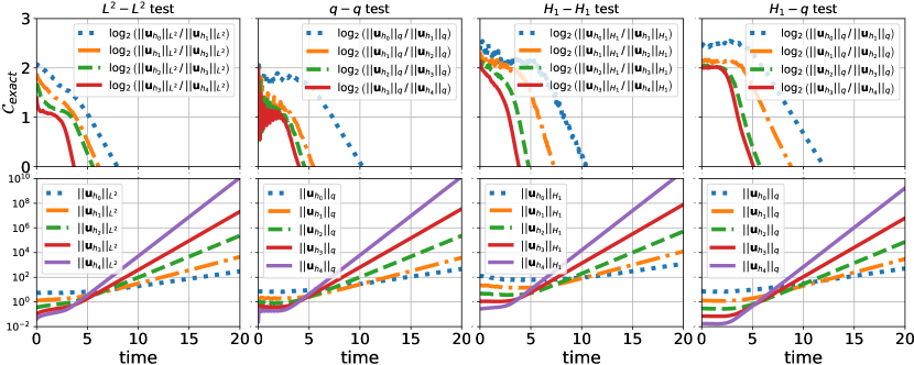
Figure 10: Our convergence tests for the CCM setup SYMH B1-WH B2. The top row shows the exact convergence rate, whereas the bottom the norms that are used to calculate it. The y axis for the bottom plots is $\log_{10}$. We clearly see that for all tests, $\mathcal{C}_{\textrm{exact}}$ moves away from the theoretical value faster with increasing resolution. This is a clear sign of loss of convergence. Furthermore, we see in the bottom row that the norms used in the calculation of $\mathcal{C}_{\textrm{exact}}$ grow exponentially and with increasing rate for bigger resolution.

In Fig. 10 we present all our tests for CCM performed with the SYMH B1 IBVP and the WH B2 CIBVP. In the top row we see the exact convergence rate $\mathcal{C}_{\textrm{exact}}$, and at the bottom the respective norms that are included in the calculation of $\mathcal{C}_{\textrm{exact}}$. In this case we do not see convergence in any of the tests, which can be explained by the fact that the respective norms increase in time, with a growth rate that increases with resolution. Therefore, the ratio between two norms calculated at different resolutions cannot be the desired constant in time. Notice that the way these tests fail is rather different from the way some earlier tests failed. Here we see complete loss of convergence, which is often called an instability—even though the simulation does not stop abruptly—whereas earlier we observed convergence at an order lower than the theoretically expected, or in a smaller norm than that of the given data.

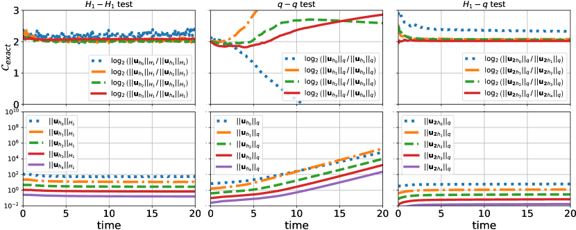
Figure 11: For comparison to the convergence of the CCM setup SYMH B1-WH B2 shown in Fig. 10, we present here the following (from left to right): the $H_{1}-H_{1}$ test for SYMH B1-SYMH B2, the $q-q$ test for WH B1-WH B2, and the $H_{1}-q$ test for the CCE setup SYMH B1-WH B2 (plotting the CIBVP norms).

For comparison, we perform the $H_{1}-H_{1}$ test for CCM between SYMH B1 and SYMH B2, the $q-q$ test for CCM with WH B1-WH B2, as well as the $H_{1}-q$ test for CCE for SYMH B1-WH B2. We chose the specific tests and combinations of PDEs, because these provided good convergence results earlier when monitoring derivative terms in the norms. The results are shown in Fig. 11. More specifically, CCM between the inhomogeneous SYMH setups exhibits the expected convergence in the $H_{1}$ norm, whereas for WH setups we see good convergence in the $q$ norm only for a brief period. The latter should not be surprising, since standard numerical methods as the ones utilized here are developed having in mind PDE problems that are strongly well posed, such as strongly or symmetric hyperbolic. These results indicate that the main source of this rapid loss of convergence is the different degree of hyperbolicity between the IBVP and CIBVP in CCM. In addition, we see good convergence in $q$ norm for the CIBVP part of CCE with SYMH B1 IBVP and WH B2 CIBVP, in line with earlier CCE results. Based on these findings, we deduce that having the influence of the bad part of the WH CIBVP solution affecting the SYMH IBVP is exactly what causes the severe loss of convergence and the rapid growth of the respective norms. When this influence is prevented by doing only CCE, this exponential growth of the norms is not present. For completeness, we have performed convergence tests for CCM with SYMH B1 IBVP and WH B2 CIBVP, with smooth given data. In complete contrast to the random noise data, the smooth data tests exhibit convergence in the $L^{2}$ norm. Note that these are not exact, but self convergence tests, since we do not know the exact solution of the tested smooth setup.

III.4.2 Synopsis

CCM provides the expected second order convergence for the solution of the composite problem, when it is performed between an IBVP and CIBVP with the same degree of hyperbolicity, that is SYMH or WH. In the case of SYMH IBVP matched with WH CIBVP, we considered two cases. In the homogeneous case, most convergence tests failed with the convergence rate reduced from second to first order; whereas in the inhomogeneous case all tests failed with the solution growing at an exponential rate that increases with increased resolution.

IV Summary and Discussion

Modeling gravitational waves at future null infinity accurately is a challenge that has to be met to obtain waveforms of high fidelity. One possibility is to successfully develop a CCM scheme for GR. Such a scheme would combine the ability to capture in detail the physics of the strong gravity regime in the Cauchy setup, with the accurate propagation of gravitational waves due to the foliation with null hypersurfaces of the characteristic setup. CCM does not suffer from artificial boundary conditions on the outer boundary of the Cauchy domain, as for instance a CCE scheme. The characteristic setup is not the only way to obtain accurate gravitational waveform models at future null infinity. Alternative strategies include hyperboloidal compactification Stewart and Friedrich (1982); Moncrief and Rinne (2009); Zenginoglu (2011); Bardeen et al. (2011); Vañó-Viñuales et al. (2015); Hilditch et al. (2018); Ansorg and Panosso Macedo (2016); Vañó-Viñuales and Husa (2018) and the use of the conformal EFEs Hübner (1999); Doulis and Frauendiener (2017); Doulis et al. (2019).

In this paper we focused on mathematical properties of CCE and CCM schemes and their impact on numerical simulations. Our motivation comes from recent progress in understanding the mathematical structure of Einstein’s field equations in the characteristic setup, in which the gauge freedom of GR is typically fixed by choosing Bondi-like coordinates which are built upon outgoing (in the case of CCE and CCM) null geodesics. In Giannakopoulos et al. (2020), certain characteristic PDE systems of GR were shown to be only weakly hyperbolic in some Bondi-like coordinates, and subsequently in Giannakopoulos et al. (2022) this structure was attributed to the choice of a Bondi-like gauge. Based on these results, it becomes clear that current CCE and CCM schemes of GR involve a strongly or symmetric hyperbolic system for the IBVP and the WH Bondi-like one in the CIBVP. Since PDE problems based on WH systems are generically not well posed, it is natural to ask whether these composite CCE and CCM setups are well posed, and to what extent should a solution based on them be trusted in making accurate predictions for gravitational waveforms.

To address this question we constructed toy models and utilized them as models for GR CCE and CCM. To address the effect of weak hyperbolicity we studied weakly and symmetric hyperbolic models for both the IBVP and the CIBVP, comparing different combinations of IBVP and CIBVP in CCE and CCM. The weakly hyperbolic structure of the CIBVP mimics that of the EFE in a Bondi-like gauge. Importantly, the WH system is constructed in such a way that it has a weakly well-posed IBVP and CIBVP. This assumption is the best possible scenario for the Bondi-like CIBVP of the EFE, involving up to second order metric derivatives. Given that there are symmetric hyperbolic characteristic formulations of GR in a Bondi-like gauge that include third order metric derivatives, one might hope to show weak well-posedness for the characteristic setups commonly used in numerical relativity. To the best of our knowledge, such a result is yet to be obtained.

For our toy models, we first studied well-posedness at the continuum level, where we considered the homogeneous case and provided energy estimates for the IBVP, CIBVP, CCE and CCM. We discussed energy estimates in norms with ($q$ and $H_{1}$) and without ($L^{2}$) derivative terms, and adapted to the IBVP, CIBVP, CCE and CCM setups. A similar analysis was performed in Giannakopoulos et al. (2020) only for the $L^{2}$ norm. As in that earlier work, we found that CCM cannot provide a well-posed PDE problem when matching a WH with a SYMH PDE problem. On the contrary, CCE can be weakly well posed if the WH problem is weakly well posed. The essential difference is in the communication of the solution between the Cauchy and the characteristic domains. In terms of the energy estimates, this is translated into a worldtube integral over the interface between the Cauchy and the characteristic domains, that is not controlled by the given data.

Based on the continuum analysis, we performed several numerical convergence tests, with a second order accurate implementation. Our main goal was to address continuous dependence of the solution on the given data, in discrete approximations to the $L^{2}$, $q$, and $H_{1}$ norms previously constructed. Our first step was to verify the expected norm convergence for the individual IBVP and CIBVP. We saw the expected convergence for the SYMH setups in the $L^{2}$ and $H_{1}$ norms and for the WH in the $q$ norm, for both the IBVP and CIBVP. An interesting scenario was realized when the given data were controlled in the $H_{1}$ norm and the convergence of the solution was tested in the $q$ norm, which is appropriate only for the WH setup. In this scenario, we observed second order convergence for both the SYMH and WH cases. Our explanation for this phenomenon is that the $H_{1}$ norm provides more control over derivatives than $q$, so the given data are appropriate for both SYMH and WH setups. Furthermore, when monitoring only the $q$ norm of the solution for the WH case we ignore the derivative terms that are responsible for the loss of convergence we see in $H_{1}$. For the SYMH case, all derivative terms converge well. In the $q$ norm, we only monitor the convergence of one of them, which dominates the norm. This scenario is crucial in understanding the reason that CCE between a SYMH IBVP and a WH CIBVP is numerically well behaved. The key point is that for $H_{1}$ controlled given data, the solution to the SYMH IBVP is also controlled in the same norm. This solution then provides boundary data for the WH CIBVP with enough control over derivative terms and so the solution to that PDE problem converges well in the $q$ norm.

The expected convergence was also seen for CCM between IBVP and CIBVP with the same degree of hyperbolicity, that is when matching SYMH to SYMH or WH to WH. In the first case, we could obtain good convergence for the solution in the $L^{2}$ and $H_{1}$ norms, for given data controlled in the same norms, respectively, whereas in the second, the same was true in the $q$ norm. When we analyzed the convergence of the solution in the $q$ norm for $H_{1}$ given data, we observed the same scenario as earlier, namely second order convergence in the $q$ norm for both SYMH-SYMH and WH-WH setups. Our understanding of this behavior is exactly the same as for the individual IBVP and CIBVP, with the only difference that in this case the various norms considered were adapted to the composite CCM PDE problem.

When matching a SYMH IBVP to a WH CIBVP we did not recover good second order convergence in any of the $L^{2}$, $q$, or $H_{1}$ norms for the solution, when the given data were controlled in the same norm. This result is in line with our expectation from the preceding continuum analysis. It is worth mentioning that as earlier, we were able to see good second order convergence in the $q$ norm when the given data were controlled in the $H_{1}$. Even though this behavior is qualitatively the same as for SYMH-WH CCE, the interpretation in terms of continuous dependence of the solution on the given data is different. In CCM, the composite IBVP-CIBVP PDE problem is treated as one and therefore the solution is controlled in a smaller norm than the given data (some derivative terms are not controlled). In CCE, this was not an issue, because we could verify convergence of the IBVP solution in the $H_{1}$ norm, for $H_{1}$ given data, and for the CIBVP solution in the $q$ norm for $H_{1}$ given data, where the latter include also given data controlled in the $q$ norm.

Our homogeneous models exhibit the same qualitative behavior for SYMH-WH CCE and CCM due to the lack of source terms. To demonstrate this, we considered an inhomogeneous example in which for the CIBVP we added a source term such that the right-moving variables which are responsible for weak hyperbolicity affect the left-moving variable, and in IBVP the left-moving variable couples to the first right-moving one. In this way, there is an interaction loop between left- and right-moving variables that is closed only when we consider CCM but not CCE. Our understanding is that when this loop is closed, it allows the part of the CIBVP solution that is influenced by the WH structure to affect in turn the IBVP solution, which consequently provides bad boundary data to the CIBVP and drives the numerical solution to explode. In our numerical experiments we see severe loss of convergence for the inhomogeneous SYMH-WH CCM setup in all norms and for all given data, even for the combination of $H_{1}$ given data and $q$ norm of the solution. In fact, we observe that the norms involved in the calculation of the convergence rate grow exponentially with time and faster for increasing resolution, which is a clear sign for loss of convergence. For comparison, we tested the inhomogeneous case for SYMH-SYMH and WH-WH CCM. In the first case we found good second order convergence in the CCM $L^{2}$ and $H_{1}$ norms for the solution, whereas in the second we saw second order convergence in the $q$ norm only for a brief initial period, the cause of which is presently unclear to us. Finally, to assess that indeed the two-way communication between the Cauchy and the characteristic domain is the crucial point in this setup, we tested the inhomogeneous SYMH-WH CCE setup for $H_{1}$ given data. In this case, we find second order convergence for the inhomogeneous WH CIBVP, exactly as in the inhomogeneous case. We interpret these results as support of our understanding of the mechanism that drives this loss of convergence, as given above.

We should highlight that we used high frequency given data in all our tests. More specifically, we used random noise with amplitude that dropped appropriately with increasing resolution. This type of data is useful in detecting WH in numerical experiments. In fact, we were able to see second order convergence in the $L^{2}$ norm for our inhomogeneous SYMH-WH CCM model, for smooth given data (see Giannakopoulos et al. (2023a)). We understand that random noise high frequency data may not be appropriate for nonuniform grids, as for instance in spectral methods. In that case, one has to construct a different type of high frequency given data. A possible suggestion could be a sinusoidal of some high but resolved frequency, that increases with increasing resolution, and an amplitude which is dropped with increasing resolution, mimicking the expected behavior of numerical error.

V Conclusions

The take home message from this analysis for current CCE setups in GR is that if the solution to the Cauchy setup is sufficiently controlled (in terms of derivatives) and provided that the WH CIBVP is weakly well posed (a strong assumption that should be firmly established) then, depending on the discretization, the numerical solution of this CCE should converge to the true solution in the limit of infinite resolution. This is another way to say that error estimates on such a solution can be trusted to an arbitrary small level (given the necessary computational resources) to provide highly accurate gravitational waveforms. Ultimately any CCE scheme is still subject to artificial boundary conditions, for which a detailed consideration is beyond our present scope.

Another lesson we take from this study is that CCM for the EFE as currently performed between a SYMH IBVP and WH CIBVP cannot be guaranteed to provide numerical approximations that converge to the true solution of the problem in the limit of infinite resolution. We do not expect the results to be changed if symmetric is replaced with strong hyperbolicity for the IBVP. Developing a strongly, if not symmetric hyperbolic characteristic formulation of the EFE seems to be necessary to move toward an implementation of GR CCM that is (strongly) well posed and properly convergent.

The supporting data for this paper, including the rest of the convergence plots and the pointwise convergence tests, are openly available from Giannakopoulos et al. (2023a, b).

VI Acknowledgments

T.G. acknowledges support from the STFC Consolidated Grant No. ST/V005596/1. D.H. was supported in part by FCT (Portugal) Project No. UIDB/00099/2020. M.Z. acknowledges financial support by the Center for Research and Development in Mathematics and Applications (CIDMA) through the Portuguese Foundation for Science and Technology (FCT – Fundação para a Ciência e a Tecnologia)—references UIDB/04106/2020 and UIDP/04106/2020—as well as FCT Projects No. 2022.00721.CEECIND, No. CERN/FIS-PAR/0027/2019, No. PTDC/FIS-AST/3041/2020, No. CERN/FIS-PAR/0024/2021, and No. 2022.04560.PTDC. This work has further been supported by the European Horizon Europe staff exchange (SE) program HORIZON-MSCA-2021-SE-01 Grant No. NewFunFiCO-101086251.

References

- Aasi et al. (2015) J. Aasi et al. (LIGO Scientific), Class. Quant. Grav. 32, 074001 (2015), arXiv:1411.4547 [gr-qc] .
- Acernese et al. (2015) F. Acernese et al. (VIRGO), Class. Quant. Grav. 32, 024001 (2015), arXiv:1408.3978 [gr-qc] .
- Akutsu et al. (2020) T. Akutsu et al. (KAGRA), (2020), 10.1093/ptep/ptaa120, arXiv:2008.02921 [gr-qc] .
- Dwyer et al. (2015) S. Dwyer, D. Sigg, S. W. Ballmer, L. Barsotti, N. Mavalvala, and M. Evans, Phys. Rev. D 91, 082001 (2015).
- Maggiore et al. (2020) M. Maggiore et al., JCAP 03, 050 (2020), arXiv:1912.02622 [astro-ph.CO] .
- Amaro-Seoane et al. (2017) P. Amaro-Seoane, H. Audley, S. Babak, J. Baker, E. Barausse, P. Bender, E. Berti, P. Binetruy, M. Born, D. Bortoluzzi, J. Camp, C. Caprini, V. Cardoso, M. Colpi, J. Conklin, N. Cornish, C. Cutler, K. Danzmann, R. Dolesi, L. Ferraioli, V. Ferroni, E. Fitzsimons, J. Gair, L. G. Bote, D. Giardini, F. Gibert, C. Grimani, H. Halloin, G. Heinzel, T. Hertog, M. Hewitson, K. Holley-Bockelmann, D. Hollington, M. Hueller, H. Inchauspe, P. Jetzer, N. Karnesis, C. Killow, A. Klein, B. Klipstein, N. Korsakova, S. L. Larson, J. Livas, I. Lloro, N. Man, D. Mance, J. Martino, I. Mateos, K. McKenzie, S. T. McWilliams, C. Miller, G. Mueller, G. Nardini, G. Nelemans, M. Nofrarias, A. Petiteau, P. Pivato, E. Plagnol, E. Porter, J. Reiche, D. Robertson, N. Robertson, E. Rossi, G. Russano, B. Schutz, A. Sesana, D. Shoemaker, J. Slutsky, C. F. Sopuerta, T. Sumner, N. Tamanini, I. Thorpe, M. Troebs, M. Vallisneri, A. Vecchio, D. Vetrugno, S. Vitale, M. Volonteri, G. Wanner, H. Ward, P. Wass, W. Weber, J. Ziemer, and P. Zweifel, “Laser interferometer space antenna,” (2017), arXiv:1702.00786 [astro-ph.IM] .
- Ruan et al. (2020) W.-H. Ruan, Z.-K. Guo, R.-G. Cai, and Y.-Z. Zhang, Int. J. Mod. Phys. A 35, 2050075 (2020), arXiv:1807.09495 [gr-qc] .
- Luo et al. (2016) J. Luo et al. (TianQin), Class. Quant. Grav. 33, 035010 (2016), arXiv:1512.02076 [astro-ph.IM] .
- Foucart et al. (2022) F. Foucart, P. Laguna, G. Lovelace, D. Radice, and H. Witek, (2022), arXiv:2203.08139 [gr-qc] .
- Bishop and Rezzolla (2016) N. T. Bishop and L. Rezzolla, Living Reviews in Relativity 19, 2 (2016).
- Duarte et al. (2022) M. Duarte, J. C. Feng, E. Gasperin, and D. Hilditch, Class. Quant. Grav. 39, 215003 (2022), arXiv:2205.09405 [gr-qc] .
- Bishop et al. (1996a) N. T. Bishop, R. Gómez, L. Lehner, and J. Winicour, Phys. Rev. D 54, 6153 (1996a).
- Bishop et al. (1997a) N. T. Bishop, R. Gómez, P. R. Holvorcem, R. A. Matzner, P. Papadopoulos, and J. Winicour, J. Comput. Phys. 136, 236 (1997a).
- Bishop et al. (1997b) N. T. Bishop, R. Gómez, L. Lehner, M. Maharaj, and J. Winicour, Phys. Rev. D 56, 6298 (1997b), gr-qc/9708065 .
- Zlochower et al. (2003) Y. Zlochower, R. Gómez, S. Husa, L. Lehner, and J. Winicour, Phys. Rev. D 68, 084014 (2003).
- Gomez et al. (2007) R. Gomez, W. Barreto, and S. Frittelli, Phys. Rev. D 76, 124029 (2007), arXiv:0711.0564 [gr-qc] .
- Babiuc et al. (2009) M. C. Babiuc, N. T. Bishop, B. Szilágyi, and J. Winicour, Phys. Rev. D 79, 084011 (2009).
- Reisswig et al. (2009) C. Reisswig, N. T. Bishop, D. Pollney, and B. Szilagyi, Phys. Rev. Lett. 103, 221101 (2009), arXiv:0907.2637 [gr-qc] .
- Reisswig et al. (2010) C. Reisswig, N. Bishop, D. Pollney, and B. Szilagyi, Class.Quant.Grav. 27, 075014 (2010), arXiv:0912.1285 [gr-qc] .
- Winicour (2012) J. Winicour, Living Rev. Relativity 15, 2 (2012), [Online article].
- Handmer and Szilagyi (2015) C. J. Handmer and B. Szilagyi, Class. Quant. Grav. 32, 025008 (2015), arXiv:1406.7029 [gr-qc] .
- Barkett et al. (2020) K. Barkett, J. Moxon, M. A. Scheel, and B. Szilágyi, Phys. Rev. D 102, 024004 (2020), arXiv:1910.09677 [gr-qc] .
- Moxon et al. (2020) J. Moxon, M. A. Scheel, and S. A. Teukolsky, Phys. Rev. D 102, 044052 (2020), arXiv:2007.01339 [gr-qc] .
- Iozzo et al. (2021a) D. A. B. Iozzo et al., Phys. Rev. D 103, 124029 (2021a), arXiv:2104.07052 [gr-qc] .
- Mitman et al. (2021) K. Mitman et al., Phys. Rev. D 103, 024031 (2021), arXiv:2011.01309 [gr-qc] .
- Iozzo et al. (2021b) D. A. B. Iozzo, M. Boyle, N. Deppe, J. Moxon, M. A. Scheel, L. E. Kidder, H. P. Pfeiffer, and S. A. Teukolsky, Phys. Rev. D 103, 024039 (2021b), arXiv:2010.15200 [gr-qc] .
- Mitman et al. (2020) K. Mitman, J. Moxon, M. A. Scheel, S. A. Teukolsky, M. Boyle, N. Deppe, L. E. Kidder, and W. Throwe, Phys. Rev. D 102, 104007 (2020), arXiv:2007.11562 [gr-qc] .
- Foucart et al. (2021) F. Foucart et al., Phys. Rev. D 103, 064007 (2021), arXiv:2010.14518 [gr-qc] .
- Moxon et al. (2021) J. Moxon, M. A. Scheel, S. A. Teukolsky, N. Deppe, N. Fischer, F. Hébert, L. E. Kidder, and W. Throwe, (2021), arXiv:2110.08635 [gr-qc] .
- Taylor et al. (2013) N. W. Taylor, M. Boyle, C. Reisswig, M. A. Scheel, T. Chu, L. E. Kidder, and B. Szilágyi, Phys. Rev. D88, 124010 (2013), arXiv:1309.3605 [gr-qc] .
- Bishop et al. (1996b) N. T. Bishop, R. Gómez, P. R. Holvorcem, R. A. Matzner, P. Papadopoulos, and J. Winicour, Phys. Rev. Lett. 76, 4303 (1996b).
- Bishop et al. (1998) N. T. Bishop, R. Gómez, R. A. Isaacson, L. Lehner, B. Szilagyi, and J. Winicour, in On the Black Hole Trail, edited by B. Bhawal and B. R. Iyer (Kluwer, Dordrecht, 1998) Chap. 24, p. 383.
- Giannakopoulos et al. (2020) T. Giannakopoulos, D. Hilditch, and M. Zilhão, Phys. Rev. D 102, 064035 (2020), arXiv:2007.06419 [gr-qc] .
- Giannakopoulos et al. (2022) T. Giannakopoulos, N. T. Bishop, D. Hilditch, D. Pollney, and M. Zilhão, Phys. Rev. D 105, 084055 (2022), arXiv:2111.14794 [gr-qc] .
- Bondi et al. (1962) H. Bondi, M. G. J. van der Burg, and A. W. K. Metzner, Proc. R. Soc. London A269, 21 (1962).
- Cao and He (2013) Z. Cao and X. He, Phys. Rev. D 88, 104002 (2013).
- Pretorius (2005) F. Pretorius, Phys. Rev. Lett. 95, 121101 (2005), gr-qc/0507014 .
- Lindblom et al. (2006) L. Lindblom, M. A. Scheel, L. E. Kidder, R. Owen, and O. Rinne, Class. Quant. Grav. 23, S447 (2006), gr-qc/0512093 .
- Lindblom et al. (2008) L. Lindblom, K. D. Matthews, O. Rinne, and M. A. Scheel, Phys. Rev. D77, 084001 (2008), arXiv:0711.2084 [gr-qc] .
- Gómez et al. (1998) R. Gómez, L. Lehner, R. Marsa, J. Winicour, A. M. Abrahams, A. Anderson, P. Anninos, T. W. Baumgarte, N. T. Bishop, S. R. Brandt, J. C. Browne, K. Camarda, M. W. Choptuik, G. B. Cook, R. Correll, C. R. Evans, L. S. Finn, G. C. Fox, T. Haupt, M. F. Huq, L. E. Kidder, S. A. Klasky, P. Laguna, W. Landry, J. Lenaghan, J. Masso, R. A. Matzner, S. Mitra, P. Papadopoulos, M. Parashar, L. Rezzolla, M. E. Rupright, F. Saied, P. E. Saylor, M. A. Scheel, E. Seidel, S. L. Shapiro, D. Shoemaker, L. Smarr, B. Szilágyi, S. A. Teukolsky, M. H. P. M. van Putten, P. Walker, and J. W. York Jr, Phys. Rev. Lett. 80, 3915 (1998), gr-qc/9801069 .
- Papadopoulos and Font (1999) P. Papadopoulos and J. A. Font, Phys. Rev. D 61, 024015 (1999).
- Siebel et al. (2002) F. Siebel, J. A. Font, E. Müller, and P. Papadopoulos, Phys. Rev. D 65, 064038 (2002).
- Garfinkle (1995) D. Garfinkle, Phys. Rev. D 51, 5558 (1995).
- Crespo et al. (2019) J. A. Crespo, H. P. de Oliveira, and J. Winicour, Phys. Rev. D100, 104017 (2019), arXiv:1910.03439 [gr-qc] .
- Gundlach et al. (2019) C. Gundlach, T. W. Baumgarte, and D. Hilditch, Phys. Rev. D 100, 104010 (2019), arXiv:1908.05971 [gr-qc] .
- Siebel et al. (2003) F. Siebel, J. A. Font, E. Müller, and P. Papadopoulos, Phys. Rev. D 67, 124018 (2003).
- Alcoforado et al. (2021) M. A. Alcoforado, W. O. Barreto, and H. P. de Oliveira, (2021), 10.1142/S0218271822500286, arXiv:2110.09640 [gr-qc] .
- Santos-Olivan and Sopuerta (2016) D. Santos-Olivan and C. F. Sopuerta, Phys. Rev. Lett. 116, 041101 (2016), arXiv:1511.04344 [gr-qc] .
- Santos-Olivan (2017) D. Santos-Olivan, Numerical Relativity studies in Anti-de Sitter spacetimes: Gravitational Collapse and the AdS/CFT correspondence, Ph.D. thesis, Barcelona U. (2017).
- Kreiss and Lorenz (1989) H.-O. Kreiss and J. Lorenz, Initial-boundary value problems and the Navier-Stokes equations (Academic Press, New York, 1989).
- Sarbach and Tiglio (2012) O. Sarbach and M. Tiglio, Living Reviews in Relativity 15 (2012), arXiv:1203.6443 [gr-qc] .
- Frittelli and Lehner (1999) S. Frittelli and L. Lehner, Phys. Rev. D 59, 084012 (1999).
- Gomez and Frittelli (2003) R. Gomez and S. Frittelli, Phys. Rev. D 68, 084013 (2003), arXiv:gr-qc/0303104 .
- Frittelli (2005) S. Frittelli, Phys. Rev. D 71, 024021 (2005), arXiv:gr-qc/0408035x .
- Rácz (2014) I. Rácz, Class. Quant. Grav. 31, 035006 (2014), arXiv:1307.1683 [gr-qc] .
- Cabet et al. (2014) A. Cabet, P. T. Chruściel, and R. T. Wafo, (2014), arXiv:1406.3009 [gr-qc] .
- Hilditch et al. (2020) D. Hilditch, J. A. Valiente Kroon, and P. Zhao, Gen. Rel. Grav. 52, 99 (2020), arXiv:1911.00047 [gr-qc] .
- Ripley (2021) J. L. Ripley, J. Math. Phys. 62, 062501 (2021), arXiv:2104.09972 [gr-qc] .
- Bezanson, Jeff and Edelman, Alan and Karpinski, Stefan and Shah, Viral B (2017) Bezanson, Jeff and Edelman, Alan and Karpinski, Stefan and Shah, Viral B, SIAM Review 59, 65 (2017).
- Giannakopoulos et al. (2023a) T. Giannakopoulos, N. T. Bishop, D. Hilditch, D. Pollney, and M. Zilhão, “Model CCE & CCM (open code),” https://github.com/ThanasisGiannakopoulos/model_CCE_CCM_public (2023a).
- Calabrese et al. (2002) G. Calabrese, J. Pullin, O. Sarbach, and M. Tiglio, Phys. Rev. D 66, 041501 (2002), gr-qc/0207018 .
- Calabrese et al. (2006) G. Calabrese, I. Hinder, and S. Husa, J. Comp. Phys. 218, 607 (2006), gr-qc/0503056 .
- Cao and Hilditch (2012) Z. Cao and D. Hilditch, Phys. Rev. D 85, 124032 (2012), arXiv:1111.2177 [gr-qc] .
- Giannakopoulos et al. (2023b) T. Giannakopoulos, N. T. Bishop, D. Hilditch, D. Pollney, and M. Zilhão, “Numerical convergence of model Cauchy-Characteristic Extraction and Matching (data),” https://zenodo.org/record/7981429 (2023b).
- Stewart and Friedrich (1982) J. M. Stewart and H. Friedrich, Proc. Roy. Soc. Lond. A 384, 427 (1982).
- Moncrief and Rinne (2009) V. Moncrief and O. Rinne, Class.Quant.Grav. 26, 125010 (2009), arXiv:0811.4109 [gr-qc] .
- Zenginoglu (2011) A. Zenginoglu, J. Comput. Phys. 230, 2286 (2011), arXiv:1008.3809 [math.NA] .
- Bardeen et al. (2011) J. M. Bardeen, O. Sarbach, and L. T. Buchman, Phys. Rev. D83, 104045 (2011), arXiv:1101.5479 [gr-qc] .
- Vañó-Viñuales et al. (2015) A. Vañó-Viñuales, S. Husa, and D. Hilditch, Class. Quant. Grav. 32, 175010 (2015), arXiv:1412.3827 [gr-qc] .
- Hilditch et al. (2018) D. Hilditch, E. Harms, M. Bugner, H. Rüter, and B. Brügmann, Class. Quant. Grav. 35, 055003 (2018), arXiv:1609.08949 [gr-qc] .
- Ansorg and Panosso Macedo (2016) M. Ansorg and R. Panosso Macedo, Phys. Rev. D93, 124016 (2016), arXiv:1604.02261 [gr-qc] .
- Vañó-Viñuales and Husa (2018) A. Vañó-Viñuales and S. Husa, Class. Quant. Grav. 35, 045014 (2018), arXiv:1705.06298 [gr-qc] .
- Hübner (1999) P. Hübner, Class. Quantum Grav. 16, 2823 (1999).
- Doulis and Frauendiener (2017) G. Doulis and J. Frauendiener, Phys. Rev. D 95, 024035 (2017), arXiv:1609.03584 [gr-qc] .
- Doulis et al. (2019) G. Doulis, J. Frauendiener, C. Stevens, and B. Whale, (2019), arXiv:1903.12482 [cs.MS] .