Mutual Information Based Pilot Design for ISAC

Abstract

The following paper presents a novel orthogonal pilot design dedicated for dual-functional radar and communication (DFRC) systems performing multi-user communications and target detection. After careful characterization of both sensing and communication metrics based on mutual information (MI), we propose a multi-objective optimization problem (MOOP) tailored for pilot design, dedicated for simultaneously maximizing both sensing and communication MIs. Moreover, the MOOP is further simplified to a single-objective optimization problem, which characterizes trade-offs between sensing and communication performances. Due to the non-convex nature of the optimization problem, we propose to solve it via the projected gradient descent method on the Stiefel manifold. Closed-form gradient expressions are derived, which enable execution of the projected gradient descent algorithm. Furthermore, we prove convergence to a fixed orthogonal pilot matrix. Finally, we demonstrate the capabilities and superiority of the proposed pilot design, and corroborate relevant trade-offs between sensing MI and communication MI. In particular, significant signal-to-noise ratio (SNR) gains for communication are reported, while re-using the same pilots for target detection with significant gains in terms of probability of detection for fixed false-alarm probability. Other interesting findings are reported through simulations, such as an information overlap phenomenon, whereby the fruitful ISAC integration can be fully exploited.

I Introduction

To address the spectrum constraint resulting from the growing demand of wireless devices, integrated sensing and communication (ISAC) systems [1, 2, 3, 4, 5, 6, 7] have recently emerged as a key enabler to solve the ever-growing spectrum congestion problem, thus attracting both the interest of academia and industry. ISAC is currently presented as one strategy to reducing this problem by co-designing wireless communication functions and radar sensing on a single hardware platform and sharing the spectrum of both radar and communication systems, thus improving band-utilization efficiency. Therefore, radar sensing and communication tasks are carried out through a unified platform and a common radio waveform at the same time, over the same frequency band, utilizing the same antennas. It is worth noting that both sensing and communication have been treated as two separate fields since the $1900$s. Then, radar waveforms performing communications have appeared, and vice-versa. For example, in $1967$, pulse interval modulation was introduced to modulate communication data onto a pulse-based radar waveform, and orthogonal frequency-division multiplexing (OFDM)-based sensing has been utilized to perform sensing with OFDM [8, 9].

Earlier research efforts were dedicated towards spectrum co-existence, also referred to as radar-communication coexistence (RCC) [10, 11, 12], whereby both radar and communication co-exist at the price of deliberate interference caused by one sub-system onto the other. Therefore, interference cancellation methods have been designed to address the RCC interference issue, such as null space projection (NSP)[13]. Unfortunately, allocating different frequency bands for these systems is neither practical nor sustainable, since both sensing and communication systems are requesting additional resources. Although being long thought of as two separate domains, sensing and communication are in fact, intimately entangled from an information-theoretic perspective [14, 15]. To realize the goal of ISAC systems, however, various obstacles must be overcome. For example, this integration complicates the design of signal waveforms, resource and hardware allocation, and network operation. All of this motivates the search for innovative approaches to these issues in order to allow the advantages of the ISAC system in real-world deployments for sensing accuracy and high-rate communications.

From a waveform design perspective, many efforts have been invested in optimizing waveforms that are deemed suitable for both sensing and communications. For instance, the design in [16] generates waveforms that minimize multi-user communication interference, while preserving some chirp characteristics with a configurable peak-to-average power ratio (PAPR). Furthermore, in [17], the authors propose a full-duplex ISAC waveform design framework to leverage the waiting time of pulsed radar for communication transmissions. In addition, a sparse vector coding-based ISAC waveform with low sidelobes and communication guarantees is proposed in [18]. Another fundamental problem for ISAC is to design appropriate beamformers to simultaneously guarantee the desired performance for both sensing amd communication. For example, the design in [19] optimizes the beamforming matrix to minimize the outage signal to interference plus noise ratio (SINR) probability, while maximizing the output radar power in the Bartlett sense. Furthermore, the authors in [20] present a framework for beyond 5G (B5G) cellular internet of things (IoT), where transmit and receive beamforming design was tailored for cochannel interference management and its impact on sensing and communications was analyzed. Moreover, the work in [21] jointly designs the beamforming matrices, along with the unmanned aerial vehicle (UAV) trajectory to maximize the overall weighted sum-rate of the system, while preserving some requirements on the beampattern gain. Besides, in [22], the authors design ISAC beamformers for delay alignment modulation (DAM) optimized for the communication signal-to-noise ratio (SNR) under some integrated sidelobe ratio (ISR) guarantees for radar sensing. The work in [23] leverages deep learning techniques to track sensing parameters within a vehicular network. Some theoretical analysis have been also conducted for ISAC systems. For example, in [24], the authors present a framework to assess the performance of certain ISAC systems, in terms of detection and false-alarm probabilities. Whereas, the work in [14] provides ISAC trade-offs in terms of Cramér-Rao bound (CRB) and communication capacity. Meanwhile, a number of research initiatives have emerged to integrate ISAC with other technologies, such as holographic multiple-input, multiple-output (MIMO) [25, 26], massive MIMO [27], reconfigurable intelligent surface (RIS) [28], simultaneously transmitting and reflecting surface (STARS) [29], OFDM [30, 31], and orthogonal time frequency space (OTFS) [32].

Nevertheless, most of the aforementioned designs focus only on waveform and beamforming designs targeting capacity, spectral efficiency, or sum-rate maximization without addressing channel estimation concerns in the context of ISAC. Therefore, we find it crucial to provide pilots, that are good for both channel estimation and target detection. To this end, this paper considers dual-functional radar and communication (DFRC) base station (BS) pilot design with flexible ISAC trade-offs, intended for downlink (DL) communication users, while listening to the backscattered echo of the transmitted pilot. Meanwhile, the users utilize the pilot for channel estimation, for equalization and decoding purposes. The design aims at maximizing mutual information, for both communication and sensing, on the Stiefel manifold in order to preserve the orthogonality constraint on the pilots. A design parameter is highlighted that trades off communication and sensing performances. Towards this ISAC design, we are faced with a non-convex optimization problem, which can be efficiently and reliably solved via an appropriate projected gradient descent algorithm. It is worth emphasizing that our results show that these pilots can be effectively utilized for channel estimation at the user’s end, while the DFRC BS can exploit the echo of the same pilot to detect targets. To that purpose, we have summarized our main contributions below.

• Gaussian mixture modeling for ISAC. Our work models the communication channel as a Gaussian mixture model (GMM), which is intended to approximate the non-Gaussian noise in wireless communication channels. Such a model is well-justified in transmissions where communication users are spatially dispensed following a non-uniform distribution. This paper is the first to push forward ISAC boundaries and promote GMM communication modeling.

• ISAC orthogonal pilot design framework. Based on the ISAC model at hand, we define key metrics based on mutual information for both sensing and communications. Furthermore, an multi-objective optimization problem (MOOP) is designed with the intention of pilot optimization, which are capable of performing simulateneous channel estimation and target detection via the same pilot waveform. Indeed, the DFRC BS can leverage the backscattered optimized pilot waveform to perform target detection via the optimal detector. Meanwhile, communication users can use the same pilot waveform to perform reliable channel estimation, followed by channel equalization and, eventually, data decoding. The framework offers ISAC trade-offs, thus enabling orthogonal pilot generation with the ability to trade communication performance with sensing, and vice-versa.

• Non-convex optimization via projected gradient descent. Being confronted with a MOOP, we first scalarize the problem, which gives rise to single-objective, but non-convex optimization problem, which is to be solved over the Stiefel manifold. We derive a projected gradient descent algorithm tailored for ISAC orthogonal pilot waveforms and prove that the method can always converge to a stable pilot solution. Convergence properties of the algorithm are derived, as well.

• Extensive simulation results. In order to highlight the various benefits of the proposed orthogonal pilot design and the potential of the designed projected gradient descent method in both multi-user communications and radar sensing, we present extensive simulation results demonstrating the potential, superiority and fruitful ISAC tradeoffs of the proposed scheme.

Furthermore, we unveil some important insights, i.e.

• The number of transmit antennas and the number of pilot symbols have profound impact on the ISAC mutual information (MI) achievable tradeoffs, allowing a flexible design of pilots, even in the presence of clutter.

• The ISAC MI performance is influenced by the target location, where the closer the target approaches the mean of communication user angle of arrival (AoA), the pointier the Pareto frontier becomes. In particular, as the target approaches the communication user, the ISAC MI frontier is pushed outwards towards the utopia point. We term this phenomenon as the information overlap phenomenon, whereby the sensing and communication channels share common information. Consequently, using the same orthogonal pilot matrix, which is designed based on the proposed method, allows to simultaneously achieve better sensing and communication MI performance.

• The receiver operating characteristic (ROC) performance of an optimized orthogonal pilot matrix for communication is better than an non-optimized orthogonal pilot matrix. The ROC performance can be further improved through a design parameter that controls the priority of sensing over communication.

• For multi-user communications, the symbol error rate (SER) performance utilizing the channel estimates aided by the generated pilot matrices exhibit gains as high as $1.6\operatorname{dB}$ for an SER level of $10^{-4}$. This gain can be controlled through an ISAC design parameter trading off sensing for communications. Furthermore, SNR gains of about $6\operatorname{dB}$ are reported for normalized mean square error (NMSE) performance of channel estimation.

The detailed structure of the following paper is given as follows. In Section II, we introduce a general ISAC system model, where both communication and sensing system models are described. Furthermore, Section III introduces mutual information metrics for the problem of pilot design, which enable us to optimize the pilots for both sensing and communication tasks. In Section IV, an optimization framework for ISAC pilot design is designed. Moreover, Section V describes a method to solve the pilot design problem in an iterative fashion, and its convergence property is described. In addition, Section VI provides numerical results to verify our analysis before concluding the paper in Section VII.

Notation: Upper-case and lower-case boldface letters denote matrices and vectors, respectively. $(.)^{T}$, $(.)^{*}$ and $(.)^{H}$ represent the transpose, the conjugate and the transpose-conjugate operators. The statistical expectation is denoted as $\mathbb{E}\{\}$. For any complex number $z\in\mathbb{C}$, the magnitude is denoted as $|z|$, its angle is $\angle z$. The $\ell_{2}$ norm of a vector $\boldsymbol{x}$ is denoted as $\|\boldsymbol{x}\|$. The matrix $\boldsymbol{I}_{N}$ is the identity matrix of size $N\times N$. The zero-vector is $\boldsymbol{0}$. For matrix indexing, the $(i,j)^{th}$ entry of matrix $\boldsymbol{A}$ is denoted by $[\boldsymbol{A}]_{i,j}$ and its $j^{th}$ column is denoted as $[\boldsymbol{A}]_{:,j}$. A positive semi-definite matrix is denoted as $\boldsymbol{A}\succeq\boldsymbol{0}$ and a vector $\boldsymbol{x}$ with all non-negative entries is denoted as $\boldsymbol{x}\succeq\boldsymbol{0}$. The all-ones vector of appropriate dimensions is denoted by $\boldsymbol{1}$.

II System Model

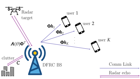
Figure 1: DFRC scenario including a DFRC BS, an intended target with clutter and $K$ communication users.

Consider an ISAC system composed of $K$ single-antenna communication users, a radar target of interest, and a DFRC BS. Let the number of transmit and receive antennas at the BS be $N_{t}$ and $N_{r}$, respectively. The communication users are considered to be located at arbitrary positions, whereas the target is supposed to be at a given angle $\theta_{0}$ from the DFRC BS. In the following, we describe the system model for both communication and radar sensing.

II-A Communication Model

Consider the DFRC BS broadcasting a pilot signal in the downlink (DL) sense over its $N_{t}$ transmit antennas. In particular, let $\boldsymbol{\Phi}\in\mathbb{C}^{L\times N_{t}}$ be the pilot matrix, to be designed, where $[\boldsymbol{\Phi}]_{\ell,n}$ represents the $\ell^{th}$ pilot symbol transmitted over the $n^{th}$ antenna. In matrix notation, we have

$$\boldsymbol{\Phi}=\begin{bmatrix}\boldsymbol{\Phi}_{1}&\ldots&\boldsymbol{\Phi}_{L}\end{bmatrix}^{T}.$$ (1)

Furthermore, let $\boldsymbol{h}_{k}$ be the channel between DFRC BS and $k^{th}$ communication user. Then, the received signal in the DL over $L<N_{t}$ instances seen at the the $k^{th}$ communication user reads

$$\boldsymbol{y}_{k}=\boldsymbol{\Phi}\boldsymbol{h}_{k}+\boldsymbol{n}_{k}.$$ (2)

In (2), $\boldsymbol{y}_{k}\in\mathbb{C}^{L\times 1}$ is the received signal vector at the $k^{th}$ user and $\boldsymbol{n}_{k}$ is background noise, assumed to be white Gaussian independent and identically distributed (i.i.d) with zero mean and a multiple of identity covariance matrix as $\mathcal{N}(0,\sigma_{k}^{2}\boldsymbol{I}_{L})$.

We adopt the GMM in order to model the communication channels between DFRC BS and the users. A GMM is a general model for multicasting, where each communication user is spatially distributed in a non-uniform geometric fashion. Even more, with a large number of mixtures, one can approximate any density with the aid of GMM [33, 34]. Typically, a GMM describes an ensemble of Gaussian distributions, whereby increasing the number of Gaussian components can contribute to better describing the channel [35]. The probability density function (PDF) of channel $\boldsymbol{h}_{m}$ is modeled as GMM, i.e. a weighted sum of Gaussian densities as follows,

$$\phi_{h}(\boldsymbol{h}_{k})=\sum\limits_{n=1}^{N_{k}}\alpha_{k,n}\phi_{n}(\boldsymbol{h}_{k}),$$ (3)

where $\phi_{n}(\boldsymbol{h}_{k})$ is the complex Gaussian distribution with mean $\boldsymbol{\mu}_{m,k}$ and covariance $\boldsymbol{R}_{k,n}$, namely $\phi_{n}(\boldsymbol{h}_{k})=\mathcal{CN}(\boldsymbol{\mu}_{k,n},\boldsymbol{R}_{k,n})$. Furthermore, $\alpha_{k,n}$ are the so-called mixing coefficients, reflecting the probability that the $n^{th}$ Gaussian component, i.e. $\phi_{n}(\boldsymbol{h}_{k})$, is active in the (3), therefore, we must have $\sum_{n=1}^{N_{k}}\alpha_{k,n}=1$, $\forall k$. Also, the number of Gaussian components modeling the $k^{th}$ communication user is $N_{k}$. Finally, as indicated in [35], the set $\{\alpha_{k,n},\boldsymbol{\mu}_{k,n},\boldsymbol{R}_{k,n}\}_{n=1}^{N_{k}}$ are the GMM parameters that model channel component $\boldsymbol{h}_{k}$.

The communication users perform channel estimation, e.g. linear minimum mean square error (MMSE) estimation, then feedback those estimates to the DFRC BS. The DFRC BS then uses those estimates to precode the modulated information as follows

$$\boldsymbol{Y}_{c}=\boldsymbol{H}\boldsymbol{W}\boldsymbol{S}_{c}+\boldsymbol{N}_{c},$$ (4)

where $\boldsymbol{H}=\begin{bmatrix}\boldsymbol{h}_{1}&\ldots&\boldsymbol{h}_{K}\end{bmatrix}^{T}$ is the communication channel matrix over all users, assumed fixed within a certain block. Moreover, $\boldsymbol{S}_{c}\in\mathbb{C}^{K\times B}$ belong to a certain constellation, e.g. $2^{p}-$ quadrature amplitude modulation (QAM) and $B$ is the block length. In addition, $\boldsymbol{W}$ is a communication precoding matrix (e.g. zero-forcing (ZF) or MMSE precoding) that utilizes the channel estimates reported by the users.

II-B Sensing Model

The radar sub-system within the DFRC system exploits the same pilot matrix as the one utilized for communication tasks, i.e. $\boldsymbol{\Phi}$. In precise, the pilots transmitted over $N_{t}$ antennas and $L$ slots are designed to satisfy both dual sensing and communication functionalities. Assuming a colocated mono-static MIMO radar setting, the received backscattered signal at the DFRC BS over $N_{r}$ receiving antennas can be written as [36]

$$\boldsymbol{Y}_{r}=\gamma_{0}\boldsymbol{a}_{N_{r}}(\theta_{0})\boldsymbol{a}_{N_{t}}^{T}(\theta_{0})\boldsymbol{\Phi}^{T}+\sum\limits_{i=1}^{Q}\gamma_{i}\boldsymbol{a}_{N_{r}}(\theta_{i})\boldsymbol{a}_{N_{t}}^{T}(\theta_{i})\boldsymbol{\Phi}^{T}+\boldsymbol{Z}_{r}.$$ (5)

The vectors $\boldsymbol{a}_{N_{r}}(\theta)\in\mathbb{C}^{N_{r}\times 1}$ and $\boldsymbol{a}_{N_{t}}(\theta)\in\mathbb{C}^{N_{t}\times 1}$ model the transmit/receive array steering vectors pointing towards angle $\theta$, respectively. For instance, if a uniform linear antenna (ULA) array setting is adopted, then the steering vectors are given as follows

$$\boldsymbol{a}_{N_{t}}(\theta) =\begin{bmatrix}1&e^{j\frac{2\pi}{\lambda}d_{t}\sin(\theta)}&\ldots&e^{j\frac{2\pi}{\lambda}d_{t}(N_{t}-1)\sin(\theta)}\end{bmatrix}^{T},$$ (6)

$$\boldsymbol{a}_{N_{r}}(\theta) =\begin{bmatrix}1&e^{j\frac{2\pi}{\lambda}d_{r}\sin(\theta)}&\ldots&e^{j\frac{2\pi}{\lambda}d_{r}(N_{r}-1)\sin(\theta)}\end{bmatrix}^{T},$$ (7)

where $\lambda$ is the wavelength and $d_{t},d_{r}$ are the inter-element spacing between transmit and receive antennas, respectively. Since a co-located setting is utilized, the angle of departure (AoD) and AoA of the backscattered component is the same.

We assume that the above reception, sampling and signal processing happen within the same time interval referred to as the coherent processing interval (CPI) [22, 37, 38], which is an interval where $\theta_{0},\theta_{1}\ldots\theta_{Q}$ and $\gamma_{0},\gamma_{1}\ldots\gamma_{Q}$ remain unchanged [6]. The CPI length depends on the mobility of objects in the channels and is typically a few milliseconds when objects move at speeds of tens of meters per second. On the other hand, the $\gamma_{i}$’s vary between different realizations of $\boldsymbol{Y}_{r}$. Therefore, following the Swerling-I model, we can assume that $\gamma_{0}\sim\mathcal{CN}(0,\nu_{0})$ [39, 40]. In addition, the $i^{th}$ clutter power is denoted as $\nu_{i}=\mathbb{E}(|\gamma_{i}|^{2})$.

Furthermore, the backscattered signal $\boldsymbol{Y}_{r}\in\mathbb{C}^{N_{r}\times L}$ is the received radar vector and $\gamma_{0}$ is the complex channel gain of the reflected echo, containing two-way delay information between the DFRC BS and the radar target of interest. The angle $\theta$ represents the AoA of the target relative to the DFRC receive array. Nevertheless, due to clutter presence, the $i^{th}$ clutter source with complex gain $\gamma_{i}$ is located at $\theta_{i}$ relative to the DFRC BS. In addition, $Q$ is the number of clutter components in the environment. The noise of the radar sub-system is i.i.d Gaussian modeled as $\boldsymbol{Z}_{r}\sim\mathcal{N}(0,\sigma_{r}^{2}\boldsymbol{I}_{N})$. In the next section, we introduce performance metrics to optimize the pilot matrix intended for both sensing and communication tasks.

III Performance Metrics

Radar waveforms are designed to enhance various sensing capabilities, such as detection, imaging and location estimation accuracy. On the other hand, communication waveforms maximize the information reliably transported between the BS and the communication users. In this study, the aim is to design a common pilot matrix to simultaneously optimize the sensing detection potential at the DFRC BS and channel estimation reliability at all communication users. In this section, we attempt to unify the communication and sensing performance metrics via appropriate mutual information based indicators.

III-A Mutual Information for Communications

The MI is a special instance of the more general quantity, that is the relative entropy, which measures the distance between probability distributions [41]. Following [41], the MI between the received DL signal at the $k^{th}$ communication user and the $k^{th}$ channel vector can be expressed as

$$I(\boldsymbol{y}_{k};\boldsymbol{h}_{k})=h(\boldsymbol{y}_{k})-h(\boldsymbol{y}_{k}|\boldsymbol{h}_{k}),$$ (8)

where $h(\boldsymbol{y}_{k})$ is the differential entropy of the received signal $\boldsymbol{y}_{k}$ and $h(\boldsymbol{y}_{k}|\boldsymbol{h}_{k})$ stands for differential entropy of $h(\boldsymbol{y}_{k})$ given $\boldsymbol{h}_{k}$. In the following, we propose an MI-based metric associated with the $k^{th}$ communication user.

Proposition 1: For a given pilot matrix $\boldsymbol{\Phi}$, the MI between $\boldsymbol{y}_{k}$ and $\boldsymbol{h}_{k}$ can be approximated as $I(\boldsymbol{y}_{k};\boldsymbol{h}_{k})\simeq\mathcal{M}_{k}^{\tt{comm}}(\boldsymbol{\Phi})$ where

$$\mathcal{M}_{k}^{\tt{comm}}(\boldsymbol{\Phi})\triangleq-\log\Big{(}\sum_{n=1}^{N_{k}}\frac{\alpha_{k,n}e^{-\beta_{k,n}(\boldsymbol{\Phi})}}{\det(\boldsymbol{\Sigma}_{k,n}(\boldsymbol{\Phi}))}\Big{)}+\tt{cnst},$$ (9)

and

$$\beta_{k,n}(\boldsymbol{\Phi}) =\bar{\boldsymbol{\mu}}_{k,n}^{H}\boldsymbol{\Phi}^{H}\boldsymbol{\Sigma}_{k,n}^{-1}(\boldsymbol{\Phi})\boldsymbol{\Phi}\bar{\boldsymbol{\mu}}_{k,n},$$ (10)

$$\bar{\boldsymbol{\mu}}_{k,n} =\sum_{n^{\prime}=1}^{N_{k}}\alpha_{k,n^{\prime}}\boldsymbol{\mu}_{k,n^{\prime}}-\boldsymbol{\mu}_{k,n},$$ (11)

$$\boldsymbol{\Sigma}_{k,n}(\boldsymbol{\Phi}) =\boldsymbol{\Phi}\boldsymbol{R}_{k,n}\boldsymbol{\Phi}^{H}+\sigma_{k}^{2}\boldsymbol{I}_{L}.$$ (12)

Furthermore, ${\tt{cnst}}$ is a term independent of $\boldsymbol{\Phi}$.

Proof: See Appendix A.

III-B Mutual Information for Sensing

We consider that the DFRC BS listens to backscattering reflections and observes the signal based on two hypothesis. The first being $\mathcal{H}_{0}$, where it assumes the absence of any target, therefore observing interference and background noise. On the other hand, the alternative hypothesis, i.e. $\mathcal{H}_{1}$, where the signal is present and is superimposed on top of interference and background noise. To this end, the DFRC listens over $L$ samples and considers the following hypothesis testing problem,

$$\begin{cases}\mathcal{H}_{0}:\qquad\boldsymbol{y}_{r}=\boldsymbol{c}+\boldsymbol{n}_{r},\\ \mathcal{H}_{1}:\qquad\boldsymbol{y}_{r}=\boldsymbol{d}+\boldsymbol{c}+\boldsymbol{n}_{r}.\end{cases}$$ (13)

For convenience, we have directly expressed the hypothesis testing problem using vectorized quantities. In particular, $\boldsymbol{y}_{r}=\operatorname{vec}(\boldsymbol{Y}_{r})\in\mathbb{C}^{N_{r}L\times 1}$, and the signal of interest, i.e. $\boldsymbol{d}$, and the clutter vector $\boldsymbol{c}$ can be expressed as

$$\boldsymbol{d} =\gamma_{0}\operatorname{vec}(\boldsymbol{a}_{N_{r}}(\theta_{0})\boldsymbol{a}_{N_{t}}^{T}(\theta_{0})\boldsymbol{\Phi}^{T})\triangleq\gamma_{0}\boldsymbol{\mu}_{0},$$ (14)

$$\boldsymbol{c} =\sum_{i=1}^{Q}\gamma_{i}\operatorname{vec}(\boldsymbol{a}_{N_{r}}(\theta_{i})\boldsymbol{a}_{N_{t}}^{T}(\theta_{i})\boldsymbol{\Phi}^{T})\triangleq\sum\limits_{i=1}^{Q}\gamma_{i}\boldsymbol{\mu}_{i}.$$ (15)

An equivalent, and more convenient, way of expressing the hypothesis test in (13) is

$$\begin{cases}\mathcal{H}_{0}:\ \boldsymbol{z}\sim\mathcal{CN}(\boldsymbol{0},\boldsymbol{I}),\\ \mathcal{H}_{1}:\ \boldsymbol{z}\sim\mathcal{CN}(\boldsymbol{0},(\boldsymbol{R}_{\boldsymbol{cc}}+\sigma_{r}^{2}\boldsymbol{I})^{-\frac{1}{2}}\boldsymbol{R}_{\boldsymbol{dd}}(\boldsymbol{R}_{\boldsymbol{cc}}+\sigma_{r}^{2}\boldsymbol{I})^{-\frac{1}{2}}+\boldsymbol{I}),\end{cases}$$ (16)

where $\boldsymbol{R}_{\boldsymbol{cc}}$ and $\boldsymbol{R}_{\boldsymbol{dd}}$ are the covariance matrices of $\boldsymbol{c}$ and $\boldsymbol{d}$, respectively. Also, $\boldsymbol{z}=(\boldsymbol{R}_{\boldsymbol{cc}}+\sigma_{r}^{2}\boldsymbol{I})^{-\frac{1}{2}}\boldsymbol{y}_{r}$. In general, the larger the MI between the parameters of interest and the observed data, the more information we have about the target of interest [42]. Based on this, we have the following MI-based performance metric for radar sensing,

Proposition 2: For a given pilot matrix $\boldsymbol{\Phi}$ and large enough number of receive antennas, i.e. $N_{r}$, the MI related to the hypothesis testing problem in (13) can be approximated as $I(\boldsymbol{Y}_{r};\boldsymbol{\Theta},\boldsymbol{\nu}|\boldsymbol{\Phi})\simeq\mathcal{M}^{\tt{sense}}(\boldsymbol{\Phi})$, where

$$\mathcal{M}^{\tt{sense}}(\boldsymbol{\Phi})\triangleq\log(1+\frac{\nu_{0}}{\sigma_{r}^{2}}\|\boldsymbol{\mu}_{0}\|^{2}-\frac{\nu_{0}}{\sigma_{r}^{2}}\sum\limits_{i=1}^{Q}\frac{\nu_{i}|\boldsymbol{\mu}_{0}^{H}\boldsymbol{\mu}_{i}|^{2}}{\sigma_{r}^{2}+\nu_{i}\|\boldsymbol{\mu}_{i}\|^{2}}).$$ (17)

Proof: See Appendix B.

The MI-based performance metric in Proposition 2 provides various insights. First, the second term appearing in the $\log$ is the contribution in the look-direction towards a target of interest located at direction $\theta_{0}$. The third term appearing within the $\log$ is due to the presence of the $Q$ clutter components. Therefore, the maximization of the proposed MI-based metric, i.e. $\mathcal{M}^{\tt{sense}}(\boldsymbol{\Phi})$, aims at maximizing the difference between the power found in the look direction and that of the clutter components, in $\log$ sense. In the next sub-section, we aim at integrating both MI-based metrics for optimizing communication and sensing performance.

IV Optimization Framework for ISAC Pilot Design

In this section, we describe an optimization framework enabling us to generate orthogonal pilots that optimize the mutual information for communication and sensing. Since multiple MI-based objectives are to be jointly optimized, an appropriate MOOP [43] can be constructed. To this end, in order to jointly optimize both communication and sensing, we consider the following problem

$$(\mathcal{P}_{\tt{MOOP}}):\begin{cases}\max\limits_{\boldsymbol{\Phi}}&\begin{bmatrix}\mathcal{M}_{1}^{\tt{comm}}(\boldsymbol{\Phi}),\ldots,\mathcal{M}_{K}^{\tt{comm}}(\boldsymbol{\Phi}),\mathcal{M}^{\tt{sense}}(\boldsymbol{\Phi})\end{bmatrix}\\ \textrm{s.t.}&\boldsymbol{\Phi}\boldsymbol{\Phi}^{H}=\boldsymbol{I}.\end{cases}$$ (18)

In equation (18), the MOOP aims at maximizing all sensing and multi-communication MIs simultaneously. This type of optimization problem appears under different names in the literature, such as a vector optimization [44, 45] or multi-criteria optimization [46, 47]. Notice that an orthogonality constraint is enforced on the pilot matrix through $\boldsymbol{\Phi}\boldsymbol{\Phi}^{H}=\boldsymbol{I}$ because orthogonal pilot patterns are commonly employed and desired for multi-channel estimation. Generally speaking, orthogonal pilot sequences represent one approach to eliminate the inter-cell interference. In addition, least squares channel estimators become straightforward to implement as no matrix inversion of $\boldsymbol{\Phi}$ will be required.

Now, since the objective function in (18) is multi-dimensional, we can transform it, utilizing a technique referred to as scalarization, with the aid of a goal function [43], hereby denoted as $\psi:\mathbb{R}^{K+1}\rightarrow\mathbb{R}$. More precisely, this goal function describes an ISAC tradeoff between the different MI-based sensing and communication objectives. There are a number of goal function options to be aware of, the simplest being the weighted-sum function, i.e. $\psi(\boldsymbol{x})=\sum_{k}w_{k}\boldsymbol{x}_{k}$. Another choice includes the geometric mean, which is useful when the underlying objectives have different numerical ranges. Since our objectives are all MI-based, hence are of the same nature, then the geometric mean function does not seem to be useful. Other choices are the weighted Chebyshev function and the distance goal function.

Adopting the scalarization technique via weighted-sum, the scalarized version of the MOOP in (18) can be written as

$$(\mathcal{P}_{\tt{s}}):\begin{cases}\max\limits_{\boldsymbol{\Phi}}&\mathcal{M}^{\tt{ISAC}}(\boldsymbol{\Phi})\triangleq\rho\mathcal{M}^{\tt{comm}}(\boldsymbol{\Phi})+(1-\rho)\mathcal{M}^{\tt{sense}}(\boldsymbol{\Phi})\\ \textrm{s.t.}&\boldsymbol{\Phi}\boldsymbol{\Phi}^{H}=\boldsymbol{I}.\end{cases}$$ (19)

where $\mathcal{M}^{\tt{comm}}(\boldsymbol{\Phi})=\sum_{k}w_{k}\mathcal{M}_{k}^{\tt{comm}}(\boldsymbol{\Phi})$ and $\sum_{k}w_{k}=1$. In the above formulation, the design parameter $\rho$ balances the ISAC tradeoff between sensing, in terms of detection performance seen through $\mathcal{M}^{\tt{sense}}(\boldsymbol{\Phi})$ and the communication channel estimation performance, which is seen through $\mathcal{M}^{\tt{comm}}(\boldsymbol{\Phi})$. In other words, increasing $\rho$ gives a higher priority onto the communication sub-system and decreasing it prioritizes sensing. For communications, the $k^{th}$ user is given a preference associated with value $w_{k}$. For equal performance along communication users, one can set $w_{1}=\ldots=w_{K}=\frac{1}{K}$. Observing problem $(\mathcal{P}_{\tt{s}})$ in (19), the cost $\mathcal{M}^{\tt{ISAC}}(\boldsymbol{\Phi})$ in conjunction with the orthogonality constraint leave us with a highly non-convex and non-linear optimization problem. In the next section, we propose an algorithm to directly solve $(\mathcal{P}_{\tt{s}})$.

V ISAC Pilot Design by Projected Gradient Descent

V-A Projected Gradient Descent over the Stiefel Manifold

Figure 2: An illustration depicting the convergence of the projected gradient descent method for ISAC pilot-design. The point $\boldsymbol{\Phi}^{\tt{opt}}$ is the optimal design matrix, which globally maximizes $\mathcal{M}^{\tt{ISAC}}(\boldsymbol{\Phi})$ on the Stiefel manifold.

We design a projected gradient descent method to optimize problem $(\mathcal{P}_{\tt{s}})$. In other words, the projected gradient descent iterates as follows

$$\boldsymbol{Z}_{t+1} =\boldsymbol{\Phi}_{t}+\gamma\nabla_{\boldsymbol{\Phi}}\mathcal{M}^{\tt{ISAC}}(\boldsymbol{\Phi})\Big{|}_{\boldsymbol{\Phi}=\boldsymbol{\Phi}_{t}},$$ (20)

$$\boldsymbol{\Phi}_{t+1} =\boldsymbol{\pi}(\boldsymbol{Z}_{t+1}),$$ (21)

where

$$\boldsymbol{\pi}(\boldsymbol{Y})=\operatorname*{arg\,min}_{\boldsymbol{X}\in{\tt{St}}(L,N_{t})}\|\boldsymbol{X}-\boldsymbol{Y}\|^{2}_{F}.$$ (22)

where ${\tt{St}}(N_{t},L)=\{\boldsymbol{X}\in\mathbb{C}^{L\times N_{t}}:\boldsymbol{X}\boldsymbol{X}^{H}=\boldsymbol{I}_{L}\}$ is the Stiefel manifold, which ”boils down” to the unit-sphere manifold for $L=1$. Note that for the case of $N_{t}>L$, $\boldsymbol{\pi}(\boldsymbol{Y})=\boldsymbol{U}\boldsymbol{I}_{L,N_{t}}\boldsymbol{V}^{H}$, where $\boldsymbol{I}_{L,N_{t}}\in\mathbb{R}^{L\times N_{t}}$ is a rectangular diagonal matrix with all of its diagonal entries set to $1$. Also $\boldsymbol{Y}=\boldsymbol{U}\boldsymbol{\Lambda}\boldsymbol{V}^{H}$ represents the singular value decomposition (SVD) operation. Observe that (20) is a classical gradient descent step and (21) projects the current intermediate point onto the closest point within the feasible set, i.e. the Stiefel manifold, via $\boldsymbol{\pi}(\boldsymbol{Y})$. In this way, any iteration of the projected gradient algorithm is guaranteed to output an orthogonal pilot, while maximizing the cost $\mathcal{M}^{\tt{ISAC}}(\boldsymbol{\Phi})$.

We now shed light on the gradients, by noting that their expressions can be computed in closed-form. Using the expression defined of $\mathcal{M}^{\tt{ISAC}}(\boldsymbol{\Phi})$ defined in (19), and with the help of (9) and (17), we can write

$$\nabla_{\boldsymbol{\Phi}}\mathcal{M}^{\tt{ISAC}}(\boldsymbol{\Phi})=\rho\sum_{k}w_{k}\nabla_{\boldsymbol{\Phi}}\mathcal{M}_{k}^{\tt{comm}}(\boldsymbol{\Phi})+(1-\rho)\nabla_{\boldsymbol{\Phi}}\mathcal{M}^{\tt{sense}}(\boldsymbol{\Phi}),$$ (23)

where the expression of $\nabla_{\boldsymbol{\Phi}}\mathcal{M}_{k}^{\tt{comm}}(\boldsymbol{\Phi})$ is given in Appendix C and the expression of $\nabla_{\boldsymbol{\Phi}}\mathcal{M}^{\tt{sense}}(\boldsymbol{\Phi})$ is given in Appendix D. At this point, the projected gradient descent method is fully defined and can be executed with the defined gradients. We now analyze the convergence properties of the iterative algorithm.

V-B Convergence Properties

Unlike classical analysis, where the cost and the projection set are assumed to be convex, this analysis studies the convergence properties of the projected gradient descent of the non-convex pilot design problem. Before we proceed, we make some assumptions regarding the structure of the function $\mathcal{M}^{\tt{ISAC}}(\boldsymbol{\Phi})$. The following definitions provide lower/upper bounds on specific classes of differentiable, and possibly non-convex, functions, namely

Definition 1: [48] A function $f:\mathbb{R}^{n}\rightarrow\mathbb{R}$ is said to be $(\alpha,\beta,\epsilon)-$ restricted strongly smooth (RSS) if it is continuously differentiable over a possibly non-convex region $\mathcal{S}\subseteq\mathbb{R}^{n}$ and for every $\boldsymbol{x}_{1},\boldsymbol{x}_{2}\in\mathcal{S}$, we have that

$$f(\boldsymbol{x}_{2})-f(\boldsymbol{x}_{1})-\nabla f^{T}(\boldsymbol{x}_{1})(\boldsymbol{x}_{2}-\boldsymbol{x}_{1})\leq\frac{\beta}{2}\|\boldsymbol{x}_{1}-\boldsymbol{x}_{2}\|^{2}+\frac{\alpha}{2}\epsilon^{2}.$$ (24)

Definition 2: [48] A function $f:\mathbb{R}^{n}\rightarrow\mathbb{R}$ is said to be $(\alpha,\epsilon)-$ restricted strongly convex (RSC) if it is continuously differentiable over a possibly non-convex region $\mathcal{S}\subseteq\mathbb{R}^{n}$ and for every $\boldsymbol{x}_{1},\boldsymbol{x}_{2}\in\mathcal{S}$, we have that

$$f(\boldsymbol{x}_{2})-f(\boldsymbol{x}_{1})-\nabla f^{T}(\boldsymbol{x}_{1})(\boldsymbol{x}_{2}-\boldsymbol{x}_{1})\geq\frac{\alpha}{2}\|\boldsymbol{x}_{1}-\boldsymbol{x}_{2}\|^{2}-\frac{\alpha}{2}\epsilon^{2}.$$ (25)

Given the RSC and RSS of a continuously differentiable function, the term $\epsilon$ captures the non-convexity of $f$ along $\mathcal{S}\subseteq\mathbb{R}^{n}$. Indeed, with $\epsilon=0$, one can see that the function is strongly convex and smooth. Hence, $\epsilon,\alpha,\beta$ can be seen as parameters that trade-off smoothness and convexity. Note that $(\alpha,\epsilon)-$RSC assumptions were also used to establish theoretical results to quantify local optima of regularized estimators, where loss/penalty function are allowed to be non-convex over its associated domain [49].

Provided these definitions, we have the following convergence result on the pilot design projected gradient descent method.

Theorem 1: For any random initialization of the pilot matrix $\boldsymbol{\Phi}_{0}$ and given $\alpha,\beta,\epsilon$ such that function $-\mathcal{M}^{\tt{ISAC}}(\boldsymbol{\Phi})$ is $(\alpha,\epsilon)-$RSC and $(\alpha,\beta,\epsilon)-$RSS, the projected gradient descent ISAC-based pilot design algorithm described in (20), (21), (22) converges to $\boldsymbol{\Phi}_{\infty}$, such that

$$\mathcal{M}^{\tt{ISAC}}(\boldsymbol{\Phi}^{{\tt{opt}}})-\mathcal{M}^{\tt{ISAC}}(\boldsymbol{\Phi}_{\infty})\leq\frac{\alpha+\frac{\beta}{2}}{1-\frac{\beta}{\alpha}}\epsilon^{2},$$ (26)

where $\boldsymbol{\Phi}^{{\tt{opt}}}$ is the global maximum of $\mathcal{M}^{\tt{ISAC}}(\boldsymbol{\Phi})$.

Proof: See Appendix E.

Therefore, Theorem 1 reveals that the projected gradient descent method converges to the true maximizer $\boldsymbol{\Phi}^{{\tt{opt}}}$, up to a certain precision level controlled by $\epsilon$. An illustration showing the points related to the projected gradient descent method is given in Fig. 2. The pilots generated by the method are projected back onto the Steifel manifold ${\tt{St}}(L,N_{t})$ to give $\boldsymbol{\Phi}_{t}$ whenever a new descent update is available, i.e. $\boldsymbol{Z}_{t-1}$.

VI Simulation Results

In this section, we carry out simulations to demonstrate the MI-based ISAC tradeoffs, as well as the performance advantages of the proposed pilot design method. The array configuration at the DFRC BS follow a ULA fashion for both transmit and receive arrays as shown given in (6) and (7). The central frequency is set to $f_{c}=5\operatorname{GHz}$. We take $N_{k}=180$ over all $K$ communication users. Following [50], the PDF of each channel component follows a GMM given in (3), where each activation probability is modeled through a Laplacian distribution, i.e. $\alpha_{k,n}=\frac{1}{\sqrt{2}\bar{\sigma}_{k}}\exp(-\frac{\sqrt{2}|\theta_{n}-\bar{\theta}_{k}|}{\bar{\sigma}_{k}})$, where $\bar{\sigma}_{k}$ is the azimuth spread characterizing the channel between the DFRC BS and the $k^{th}$ communication user. Also, $\bar{\theta}_{k}$ represents the mean AoA of the spread of the channel towards the $k^{th}$ user. Each Gaussian component of the GMM is assumed to have a covariance matrix $\boldsymbol{R}_{k,n}=\int_{\mathcal{R}_{n}}\boldsymbol{a}_{N_{t}}(\theta)\boldsymbol{a}_{N_{t}}^{H}(\theta)\ d\theta$, where $\mathcal{R}_{n}$ is the region of over which the $n^{th}$ GMM component is assumed to be observed. These regions are assumed to be disjoint and $\bigcup_{n}\mathcal{R}_{n}$ covers $[-90^{\circ},+90^{\circ}]$. Therefore, to generate a random realization of channel $\boldsymbol{h}_{k}$, we first generate $N_{k}=180$ Gaussian random realizations, where the $n^{th}$ component has mean $\boldsymbol{\mu}_{k,n}$ and co-variance matrix $\boldsymbol{R}_{k,n}$, then $\boldsymbol{h}_{k}$ is picked based on the activation probabilities $\alpha_{k,n}$. For the single-user case, i.e. $K=1$, we set the mean AoA component to $\bar{\theta}_{1}=70^{\circ}$. For the multi-user case, where we have set $K=4$, we assume that $\bar{\theta}_{2}=23^{\circ}$, $\bar{\theta}_{3}=-23^{\circ}$, and $\bar{\theta}_{4}=-70^{\circ}$. All communication users are treated equally, therefore $w_{k}=\frac{1}{K}$. Unless otherwise stated, the projected gradient descent algorithm runs with a step size of $\gamma=0.1$.

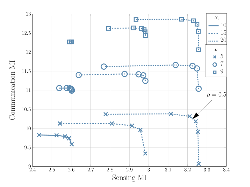
Figure 3: Achievable sensing and communication MI values for the single-user case by projected gradient descent optimization for different values of $N_{t}$ and $L$. The number of receive antennas is set to $N_{r}=5$. The target is located at $\theta_{0}=60^{\circ}$. The radar noise is $\sigma_{r}=2$ and the communication noise is $\sigma_{1}=0.1$. No clutter is considered here.

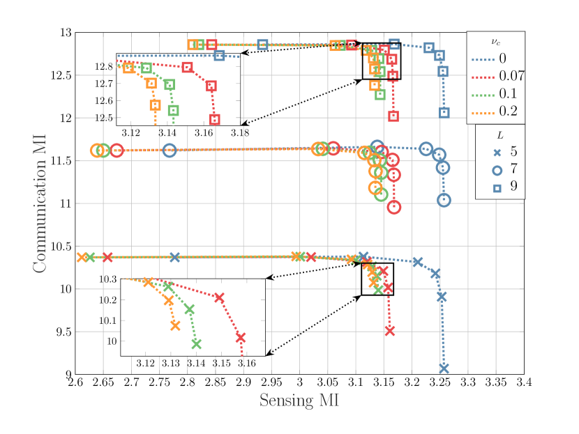
Figure 4: Clutter impact on the MI ISAC performance for the single-user case and different clutter power $\nu_{c}$ and values of $L$. We set $\theta_{1}=0^{\circ}$, $N_{r}=5$, $\theta_{0}=60^{\circ}$, $\sigma_{r}=2$ and $\sigma_{1}=0.1$.

Impact of $N_{t}$ and $L$ on the MI ISAC trade-off

In Fig. 3, we study the impact of number of transmit antennas, $N_{t}$ and number of pilot symbols (pilot length) $L$ on the sensing and communication mutual information. For fixed $L$ and with increasing number of transmit antennas, we can see that both sensing and communication mutual information improve. For example, fixing $L=5$, we see that maximum communication MI improves from $9.82$ bits to $10.12$ bits when increasing $N_{t}$ from $10$ to $15$ antennas, while the maximum sensing MI rises from $2.6$ to $2.98$ bits. The same observation is noticed when going from $N_{t}=15$ to $N_{t}=20$ for $L=5$. We set $\sigma_{r}=2$. We assume that the single-user communication noise is $\sigma_{1}=0.1$. Furthermore, the azimuth spread is set to $\bar{\sigma}_{1}=6^{\circ}$. Moreover, the target is located at $\theta_{0}=60^{\circ}$, and the number of receive antennas is set to $N_{r}=5$. Another point worth highlighting is the point corresponding to $\rho=0.5$, where we have equal priority on communication and sensing performance. We also observe that increasing $N_{t}$ also contributes to a simultaneous increase in both communication and sensing MI. For $\rho=0.5$, we observe that for $L=5$, the sensing MI increases from $2.56$ bits to $3.21$ bits, while the communication MI increases from $9.78$ bits to $10.31$ bits, when doubling the number of transmit antennas from $10$ to $20$. Another factor contributing to the joint ISAC MI gain is $L$. For instance, focusing on the point corresponding to $\rho=0.5$ and fixing $N_{t}=15$, we observe that the sensing MI increases from $2.91$ bits to $2.99$ bits, whereas the communication MI increases from $10.06$ bits to $12.58$ bits, when $L$ increases from $5$ to $9$. An interesting phenomenon worth highlighting is the achievable range of ISAC tradeoffs, as a function of $N_{t}$ and $L$. For example, when $L=9$, we notice that increasing $N_{t}$ not only improves the ISAC MI, but also allows the designer to achieve a wider set of sensing and communication MI values for different ISAC pilot matrices. Indeed, notice that for $N_{t}=10$ and $L=9$, the trade-off achieves sensing MI values that are within $[2.59,2.61]$, whereas communication MI values are within $[12.265,12.27]$. Both range of values can be increased by increasing $N_{t}$, thus allowing for more ISAC trade-offs.

Impact of clutter on the MI ISAC trade-off

In Fig. 4, we highlight how clutter can influence the ISAC performances from a mutual information perspective. The same simulation parameters as in Fig. 3, with the exception of the clutter setting. In particular, to study the impact of clutter, we set $Q=1$ and denote $\nu_{c}=\nu_{1}$. We vary the values of $\nu_{c}$ to analyze the clutter impact. The clutter is assumed to be located at $\theta_{1}=0^{\circ}$. We can see that for fixed $N_{t}$ and $L$, an increase in $\nu_{c}$ causes the sensing MI to decrease without majorly impacting the communication MI. Despite the presence of clutter, we see that the sensing MI is still relatively high enough, hence detection can still be reliably performed. Fixing $L$ to $5$, we see that a clutter component with $\nu_{c}=0.07$ deteriorates the maximal sensing MI from $3.25$ to $3.16$ bits compared to the no-clutter case. On the other hand, the maximal communication MI is at $10.37$ bits regardless of the clutter power. When equal priority is set on sensing and communication, increasing $L$ can aid in improving the sensing performance. For example, the sensing MI increases from $3.14$ to $3.16$ bits when increasing $L$ from $5$ to $9$. Similar observations can be reported for increasing $\nu_{c}$.

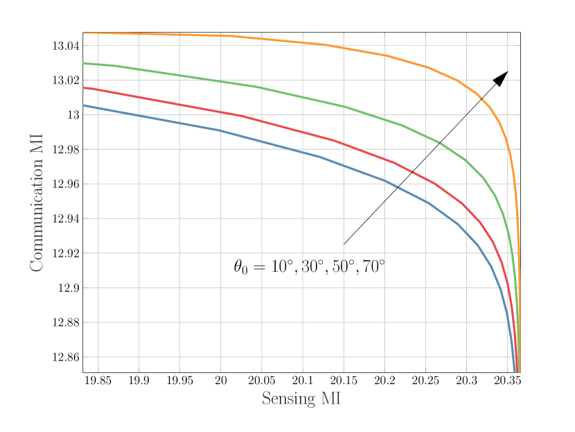
Figure 5: The impact of the target AoA on the ISAC trade-off for the single-user case. We plot $4$ MI-frontiers where the blue frontier corresponds to $\theta_{0}=10^{\circ}$ and the orange corresponds to $\theta_{0}=70^{\circ}$. We set $N_{r}=70$, $L=10$. We have $\sigma_{1}=0.1$ and $\sigma_{r}=0.002$. The user is located around $\bar{\theta}_{1}=70^{\circ}$.

Target location can improve MI ISAC gains

In Fig. 5, we aim at studying the target position and its impact on the sensing and communication MI tradeoffs. The single-user case is assumed with $L=10$ and number of receive antennas $N_{r}=70$ at the DFRC BS. We set $\sigma_{1}=0.1$ and $\sigma_{r}=0.002$. The frontiers are generated by sweeping over multiple values of $\rho$. The different frontiers are generated by changing the target’s location. The user is located around $\bar{\theta}_{1}=70^{\circ}$. In particular, we vary the target AoA by bringing it closer towards the mean of the communication user AoA. Indeed, the closer the target is brought towards the user, the boundary approach a utopia point, i.e. achieving maximal sensing and communication MI performance with the same orthogonal pilot symbols. This can be explained by some sensing and communication information overlap between the communication channel $\boldsymbol{h}_{k}$ and part of the sensing channel characterized by the AoAs $\boldsymbol{\Theta}$ and the path gains $\boldsymbol{\nu}$. Note that a similar phenomenon is reported in [14], where a sensing and communication subspace overlap can also improve communication-rate and sensing performance. The study, herein, serves as a complementary one as pilots can provide better channel estimates when the target approaches the communication user. The best performance is observed when the target and communication user are at the same location, which is an interesting use case when the objective is to sense a communication user, hence the integration gain is fully exploited.

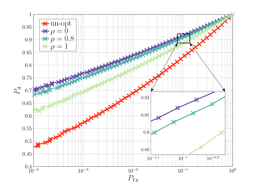
Figure 6: Receiver operating characteristic curves for different values of $\rho$ and for an non-optimized and orthogonal pilot, i.e. random but orthogonal, for $\sigma_{r}=2$. The single-user case is considered with $N_{t}=20$ and $N_{r}=5$ antennas. The pilot length is $L=9$. The target is located at $\theta_{0}=60^{\circ}$ and $\sigma_{1}=0.1$.

ROC performance of pilot matrices

In Fig. 6, we take a step further and utilize the generated pilot symbols to evaluate the performance of the ROC via the optimal detector reported in [51]. In particular, the figure shows the ROC curves for different values of $\rho$ and compares the ROC performance to an non-optimized and orthogonal pilot matrix. To this end, we set the pilot length is $L=9$. Moreover, the number of transmit and receive antennas at the DFRC BS are set to $N_{t}=20$ and $N_{r}=5$ antennas, respectively. It is clear that optimizing the pilot matrix via the proposed projected gradient method can improve the detection capabilities performed at the DFRC through the same pilot matrix used for communications. For this simulation, the target is located at $\theta_{0}=60^{\circ}$ and the communication noise level is $\sigma_{1}=0.1$. As an example, if the designer sets a probability of false alarm at $P_{\tt{fa}}=10^{-4}$ and generates an orthogonal pilot matrix by the proposed method for $\rho=1$ (communication-optimal), the achieved probability of detection is $P_{\tt{d}}=0.61$, which is greater than that of an non-optimized orthogonal pilot, which achieves $P_{\tt{d}}=0.475$. Note that, even though the priority is set to the communication task (i.e. channel estimation), the optimized pilot generated by the proposed method can still outperform an non-optimized one. If the designer seeks a better detection performance, then this can be achieved by lowering $\rho$, hence giving more priority towards sensing. Indeed, with $\rho=0.8$ and for the same $P_{\tt{fa}}=10^{-4}$, the $P_{\tt{d}}$ increases from $0.61$ to $0.68$ and can reach $P_{\tt{d}}=0.7$ for $\rho=1$. Similar observations are noticed for any false-alarm probability.

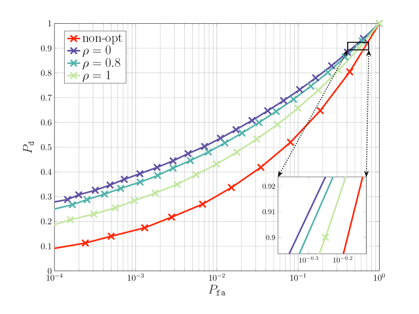
Figure 7: Receiver operating characteristic curves for different values of $\rho$ and for an non-optimized and orthogonal pilot for $\sigma_{r}=4$. All other simulation parameters are the same as those in Fig. 6.

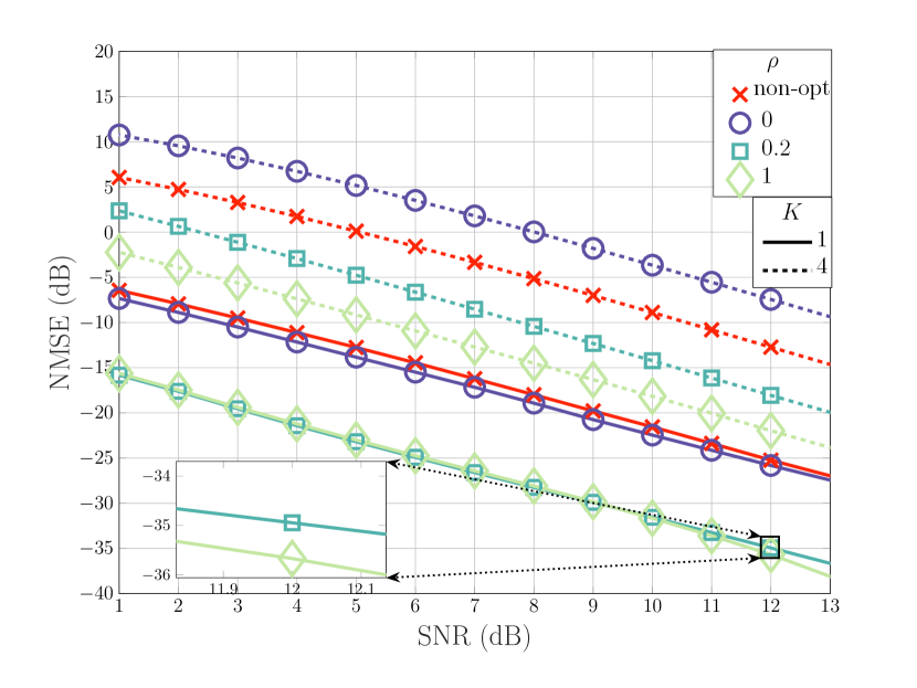
Figure 8: NMSE performance of the generated pilots compared to an unoptimized orthogonal pilot matrix for different number of communication users and different values of $\rho$.

In Fig. 7, we increase the radar noise to $\sigma_{r}=4$. All other simulation parameters are exactly the same as those in Fig. 6. Indeed, due to a more noisy radar sub-system, the detector has to increase the probability of false alarm to achieve the same detection probability performance as those specified in Fig. 6 (i.e. $\sigma_{r}=2$) for $P_{\tt{d}}=0.475$. Given that, increasing the $P_{\tt{fa}}$ level to $P_{\tt{fa}}=5\times 10^{-2}$, the non-optimized pilot achieves $P_{\tt{d}}=0.475$, whereas the proposed method for $\rho=1$ generates an orthogonal pilot with $P_{\tt{d}}=0.59$ capabilities. If a larger detection probability is desired, one would have to decrease $\rho$ thus achieving $P_{\tt{d}}=0.64$ for $\rho=0.8$ and $P_{\tt{d}}=0.67$ for $\rho=1$. We have identical observations for different false-alarm levels.

NMSE performance

In Fig. 8, we assess the NMSE performance of the generated orthogonal pilot matrices in order to study its channel estimation capability with different number of communication users, i.e. $K$, and different values of $\rho$. To this end, the NMSE is evaluated as

$$\operatorname{NMSE}=\frac{1}{KR}\sum_{k=1}^{K}\sum_{r=1}^{R}\frac{\|\boldsymbol{h}_{k,r}-\widehat{\boldsymbol{h}}^{\tt{MMSE}}_{k,r}\|^{2}}{\|\boldsymbol{h}_{k,r}\|^{2}},$$ (27)

where $\boldsymbol{h}_{k,r}$ is the communication channel between the DFRC BS and the $k^{th}$ user generated at the $r^{th}$ Monte-Carlo trial, and $\widehat{\boldsymbol{h}}^{\tt{MMSE}}_{k,r}$ is its MMSE estimate, which is a widely adopted figure of merit in signal processing [52]. As a reminder, the MMSE estimate minimizes $\mathbb{E}(\|\boldsymbol{h}_{k,r}-\widehat{\boldsymbol{h}}_{k,r}\|^{2})$ with respect to $\widehat{\boldsymbol{h}}_{k,r}$ and is obtained via the following marginalization as follows [53]

$$\begin{split}\widehat{\boldsymbol{h}}^{\tt{MMSE}}_{k,r}&\triangleq\mathbb{E}({\boldsymbol{h}}_{k,r}|\boldsymbol{y}_{k,r})\\ &=\sum\limits_{n=1}^{N_{k}}p_{k,n,r}(\boldsymbol{\mu}_{k,n}+\boldsymbol{R}_{k,n}\boldsymbol{\Phi}^{H}\boldsymbol{\Sigma}^{-1}_{k,n}(\boldsymbol{\Phi})(\boldsymbol{y}_{k,r}-\boldsymbol{\Phi}\boldsymbol{\mu}_{k,n})),\end{split}$$ (28)

where $\boldsymbol{y}_{k,r}\in\mathbb{C}^{L\times 1}$ is the received signal at the $k^{th}$ user on the $r^{th}$ trial following (2). Moreover, $\boldsymbol{\Sigma}_{k,n}(\boldsymbol{\Phi})$ is given in equation (12). The probabilities at the $r^{th}$ trial $p_{k,n,r}$ (also referred to as responsibilities) are computed via

$$p_{k,n,r}=\frac{\alpha_{k,n}\mathcal{CN}(\boldsymbol{y}_{k,r};\boldsymbol{\Phi}\boldsymbol{\mu}_{k,n},\boldsymbol{\Sigma}_{k,n}(\boldsymbol{\Phi}))}{\sum_{n^{\prime}=1}^{N_{k}}\alpha_{k,n^{\prime}}\mathcal{CN}(\boldsymbol{y}_{k,r};\boldsymbol{\Phi}\boldsymbol{\mu}_{k,n^{\prime}},\boldsymbol{\Sigma}_{k,n^{\prime}}(\boldsymbol{\Phi}))}.$$ (29)

Fig. 8 shows the resulting NMSE performance for the single-user case and multi-user (e.g. $K=4$) case. We have set $L=10$. The target is located at $\theta_{0}=-20^{\circ}$. The azimuth spread is set to $\bar{\sigma}_{k}=4^{\circ}$ per user. The number of transmit and receive antennas are set to $N_{t}=40$ and $N_{r}=70$ antennas. Analyzing the single-user case, we see that the NMSE performance of the non-optimized pilot matrix is very close to the pilot matrix generated by the proposed method for $\rho=0$ (sensing-optimal). Increasing $\rho$ to $0.2$ generates performance close to the communication-optimal pilot matrix ($\rho=1$) which gives a gain of about $6\operatorname{dB}$ as compared to the non-optimized pilot matrix. For the multi-user case at $K=4$, we can observe a more interesting phenomenon. Even though the sensing-optimal performance worse than the non-optimized pilot matrix, roughly by $2\operatorname{dB}$, a wider range of trade-offs can be achieved. For example, for $\rho=0.2$, we can gain an $\operatorname{NMSE}$ of about $3\operatorname{dB}$ and again a gain of about $6\operatorname{dB}$ when tuning for a communication-optimal orthogonal pilot matrix, i.e. $\rho=1$.

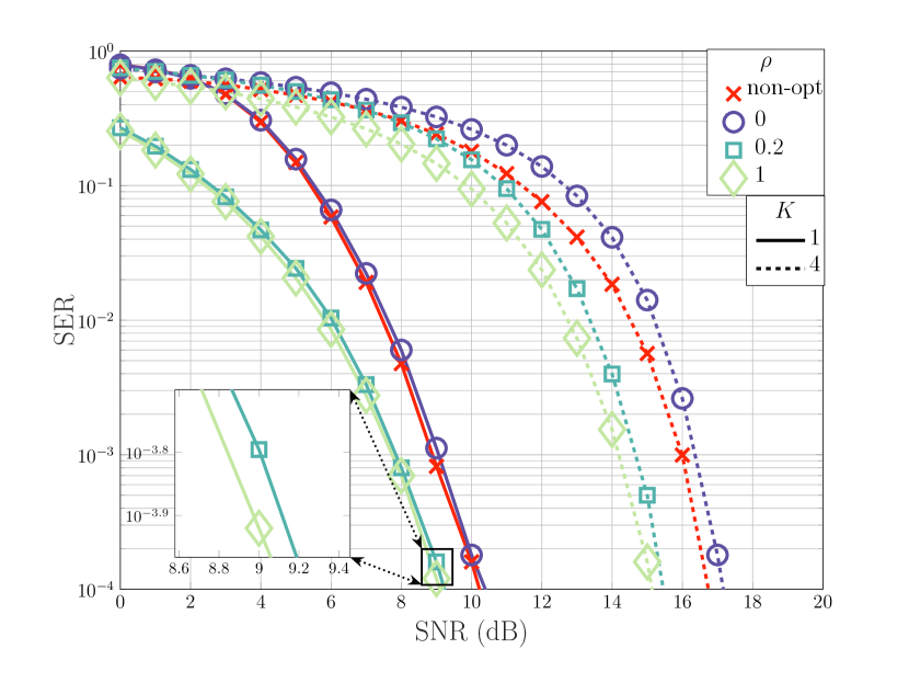
Figure 9: SER performance of the generated pilots compared to an unoptimized orthogonal pilot matrix for different values of $\rho$ and different number of communication users. A $64-$QAM with Gray encoding is used for data modulation.

SER performance

In Fig. 9, we evaluate the SER performance of the generated orthogonal pilot matrices and observe the gains in SER as compared to the non-optimized pilot matrix as a function of SNR and for different values of $\rho$ and number of communication users, i.e. $K$. The same simulation parameters are used as those in Fig. 8. For communications, a $64-$QAM was used as constellation for digital modulation with gray encoding. The MMSE channel estimator in (28) and (29) is first utilized to estimate the channel, then a ZF equalizer is used to demodulate the symbol using a hard-decision decoder. For the single-user case, and setting the SER level to $10^{-4}$, we see that the SER performance of the non-optimized pilot matrix is $0.15\operatorname{dB}$ better than that of the pilot matrix generated by the proposed method for $\rho=0$ (sensing-optimal). We can improve the SER by $1\operatorname{dB}$ by increasing $\rho$ to $0.2$. An additional gain of about $0.1\operatorname{dB}$ can be achieved by increasing $\rho$ to $1$. As for the multi-user case for $K=4$, better gains can be reported, even though the non-optimized pilot gains $0.5\operatorname{dB}$ as compared to pilot matrix generated by the proposed method for $\rho=0$. For example, setting the SER level to $10^{-4}$ and $\rho=0.2$, we can gain $1.3\operatorname{dB}$ of SNR as compared to the non-optimized pilot and $1.6\operatorname{dB}$ if we fix $\rho=1$. Therefore, we can report more SNR gains with increasing number of communication users.

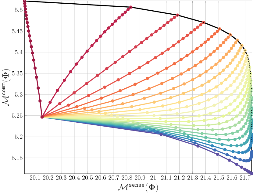
Figure 10: The convergence behavior of the proposed method in terms of $\mathcal{M}^{\tt{comm}}(\boldsymbol{\Phi})$ and $\mathcal{M}^{\tt{sense}}(\boldsymbol{\Phi})$. Each colored path represents the path taken for a fixed $\rho$. Each point corresponds to a pilot matrix generated by the method. The initial point at $(20.15,5.24)$ is the initial point shared for all paths. The paths joining the initial point with the upper left corner point and the initial point with the lower right corner point corresponds to $\rho=1$ and $\rho=0$, respectively.

Convergence Behaviour

In Fig. 10, we study the convergence behavior of the proposed method for different values of $\rho$, in terms of $\mathcal{M}^{\tt{sense}}(\boldsymbol{\Phi})$ and $\mathcal{M}^{\tt{comm}}(\boldsymbol{\Phi})$. For the sake of illustration and presentation, we pick the same initial pilot for different $\rho$ to study the path taken by the proposed projected gradient descent algorithm. For simplicity, we assume a single-user case, where the simulation parameters are the same as the single-user case in Fig. 8. The communication noise level is set to $\sigma_{1}=0.2$. The step-size is set to $\gamma=0.1$. The illustration was generated for each $\rho$ by running the proposed method, storing each generated pilot per iteration, and subsequently computing $\mathcal{M}^{\tt{comm}}(\boldsymbol{\Phi})$ with the help of (9) and $\mathcal{M}^{\tt{sense}}(\boldsymbol{\Phi})$ via (17). Therefore, each path corresponds to a different values of $\rho$. We have $21$ paths simulated by increasing $\rho$ a value of $0.05$ each time. We can see that for any $\rho$, the proposed method is guaranteed to converge to a fixed point. It is interesting to observe that all paths converge to a stable frontier. For instance, when $\rho=0$, the method converges to an orthogonal pilot matrix whose sensing and communication MI values are $(21.75,5.11)$ and $(21.75,5.16)$ for $\rho=0.05$. When $\rho=0.5$, we converge to $(21.72,5.37)$ and $(20.02,5.52)$ when $\rho=1$.

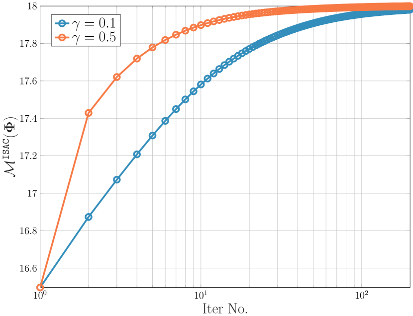
Figure 11: The impact of the step size on the convergence behavior of the projected gradient descent for ISAC pilot design.

Next, in Fig. 11, we plot the cost convergence versus the iteration number. We run the algorithm for $200$ iterations and for different values of step-size, $\gamma$. We see that for both values of $\gamma$, the method converges to a stable value of $\mathcal{M}^{\tt{ISAC}}(\boldsymbol{\Phi})=18$. Moreover, when $\gamma=0.5$, the convergence is reported to be faster as the method can converge with about $50$ iterations.

VII Conclusions and Research Directions

This paper formulated a thorough ISAC framework for designing orthogonal pilots tailored for communication and sensing purposes. With the help of mutual information quantities, we designed orthogonal pilots that are optimized for both communication and target detection. For this, a multi-objective optimization problem has been formulated to model the pilot design problem at hand. Nevertheless, a scalarization procedure was adopted, followed by an algorithmic description based on projected gradient descent was derived to generate our ISAC orthogonal pilots. Our analysis also reveals that the proposed design is guaranteed to converge to a stable orthogonal pilot. In addition, simulation results unveil the full dual potential of the design pilots, as well as the ISAC tradeoffs the framework has to offer.

Future research will be oriented towards pilot generation with additional practical properties, such as good synchronization properties and low PAPR. A possible direction may also be to utilize artificial intelligence and deep learning techniques for pilot generation, offering various features, which include but are not limited to multi-target detection and channel tracking.

Appendix A Expression of $\mathcal{M}_{k}^{\tt{comm}}(\boldsymbol{\Phi})$

This part of the appendix re-writes the mutual information between the received signal at the $k^{th}$ communication user and the channel between the DFRC BS and the $k^{th}$ communication user. To this end, we have the following set of equalities and approximations

$$\begin{split}&I(\boldsymbol{y}_{k};\boldsymbol{h}_{k})\\ &=h(\boldsymbol{y}_{k})-h(\boldsymbol{y}_{k}|\boldsymbol{h}_{k})\\ &\mathrel{\overset{\makebox[0.0pt]{\mbox{\tiny(a)}}}{=}}-\mathbb{E}\big{(}\log\phi_{y}(\boldsymbol{y}_{k})\big{)}-\mathbb{E}\big{(}\log\phi_{y}(\boldsymbol{y}_{k}|\boldsymbol{h}_{k})\big{)}\\ &\mathrel{\overset{\makebox[0.0pt]{\mbox{\tiny(b)}}}{\simeq}}-\mathbb{E}\Big{(}\log\phi_{y}(\bar{\boldsymbol{y}}_{k})+\boldsymbol{d}^{H}(\bar{\boldsymbol{y}}_{k})[\boldsymbol{y}_{k}-\bar{\boldsymbol{y}}_{k}]\Big{)}-\mathbb{E}\big{(}\log\phi_{y}(\boldsymbol{y}_{k}|\boldsymbol{h}_{k})\big{)}\\ &\mathrel{\overset{\makebox[0.0pt]{\mbox{\tiny(c)}}}{=}}-\log\phi_{y}(\bar{\boldsymbol{y}}_{k})-\boldsymbol{d}^{H}(\bar{\boldsymbol{y}}_{k})[\mathbb{E}(\boldsymbol{y}_{k})-\bar{\boldsymbol{y}}_{k}]-\mathbb{E}\big{(}\log\phi_{y}(\boldsymbol{y}_{k}|\boldsymbol{h}_{k})\big{)}\\ &\mathrel{\overset{\makebox[0.0pt]{\mbox{\tiny(d)}}}{=}}-\log\Big{(}\sum\limits_{n=1}^{N_{k}}\alpha_{k,n}\phi_{n}(\bar{\boldsymbol{y}}_{k})\Big{)}-\mathbb{E}\big{(}\log\phi_{y}(\boldsymbol{y}_{k}|\boldsymbol{h}_{k})\big{)}\\ &\mathrel{\overset{\makebox[0.0pt]{\mbox{\tiny(e)}}}{=}}-\log\Big{(}\sum_{n=1}^{N_{k}}\frac{\alpha_{k,n}\exp(-\bar{\boldsymbol{\mu}}_{k,n}^{H}\boldsymbol{\Phi}^{H}\boldsymbol{\Sigma}_{k,n}^{-1}(\boldsymbol{\Phi})\boldsymbol{\Phi}\bar{\boldsymbol{\mu}}_{k,n})}{\det(\boldsymbol{\Sigma}_{k,n}(\boldsymbol{\Phi}))}\Big{)}+\tt{cnst}.\end{split}$$ (30)

In (30), step (a) follows from the definition of differential entropy and conditional differential entropy, respectively. Note that $\phi_{y}$ is the PDF describing random variable $\boldsymbol{y}_{k}$, i.e. $\boldsymbol{y}_{k}\sim\phi_{y}$. Step (b) linearizes the $\log$ function through a $1^{st}$ order Taylor expansion around the mean of ${\boldsymbol{y}}_{k}$, i.e.

$$\bar{\boldsymbol{y}}_{k}=\mathbb{E}({\boldsymbol{y}}_{k})=\sum_{n=1}^{N_{k}}\alpha_{k,n}\boldsymbol{\Phi}\boldsymbol{\mu}_{k,n},$$ (31)

where $\boldsymbol{d}(\boldsymbol{y})$ is the gradient of $\log\phi_{y}(\boldsymbol{y})$ with respect to $\boldsymbol{y}$. Step (c) applies the expectation onto random variable $\boldsymbol{y}_{k}$. Step (d) uses $\bar{\boldsymbol{y}}_{k}\triangleq\mathbb{E}({\boldsymbol{y}}_{k})$ and uses the fact that $\boldsymbol{y}_{k}$ is also a GMM, whose PDF is given as

$$\phi_{y}(\boldsymbol{y}_{k})=\sum\limits_{n=1}^{N_{k}}\alpha_{k,n}\phi_{n}(\boldsymbol{y}_{k}),$$ (32)

where it is easy to show that each Gaussian component $\phi_{n}$ is $\phi_{n}(\boldsymbol{y}_{k})=\mathcal{CN}(\boldsymbol{\Phi}\boldsymbol{\mu}_{k,n},\boldsymbol{\Sigma}_{k,n}(\boldsymbol{\Phi}))$, and the expression of $\boldsymbol{\Sigma}_{k,n}(\boldsymbol{\Phi})$ is given in (12). Furthermore, we evaluate $\phi_{y}(\boldsymbol{y})$ in (32) at $\bar{\boldsymbol{y}}_{k}$ given in (31) to obtain $\phi_{n}(\bar{\boldsymbol{y}}_{k})$ in step (d) in (30). Indeed, after some straightforward linear algebra, we can show

$$\phi_{n}(\bar{\boldsymbol{y}}_{k})=\frac{1}{\pi^{L}\det(\boldsymbol{\Sigma}_{k,n}(\boldsymbol{\Phi}))}\times\exp(-\bar{\boldsymbol{\mu}}_{k,n}^{H}\boldsymbol{\Phi}^{H}\boldsymbol{\Sigma}_{k,n}^{-1}(\boldsymbol{\Phi})\boldsymbol{\Phi}\bar{\boldsymbol{\mu}}_{k,n}),$$ (33)

where the expression of $\bar{\boldsymbol{\mu}}_{k,n}$ is given in (11). Finally, injecting (33) in the first term of step (d) in (30), we arrive at step (e), where ${\tt{cnst}}=L\log\pi-L\log(\pi\sigma_{k}^{2}e)$. The first term in ${\tt{cnst}}$ is due to the $\pi^{L}$ appearing in the denominator of (33), whereas the second term is due to the fact that the differential entropy conditioned over the channel can be written as $\mathbb{E}\big{(}\log\phi_{y}(\boldsymbol{y}_{k}|\boldsymbol{h}_{k})\big{)}=\mathbb{E}\big{(}\log\phi_{y}(\boldsymbol{y}_{k}-\boldsymbol{\Phi}\boldsymbol{h}_{k}|\boldsymbol{h}_{k})\big{)}=\mathbb{E}\big{(}\phi_{n}(\boldsymbol{n}_{k}|\boldsymbol{h}_{k}))=-L\log(\pi\sigma_{k}^{2}e)$, since $\boldsymbol{n}_{k}$ is a complex Gaussian distribution.

Appendix B Expression of $\mathcal{M}^{\tt{sense}}(\boldsymbol{\Phi})$

In this appendix, we express the mutual information for sensing in terms of power quantities of the target of interest and clutter, as well as the cross-correlations between target of interest and the clutter. Therefore, we have the following set of equalities

$$\begin{split}&\mathcal{M}^{\tt{sense}}(\boldsymbol{\Phi})\\ &\triangleq I(\boldsymbol{Y}_{r};\boldsymbol{\Theta},\boldsymbol{\nu}|\boldsymbol{\Phi})\mathrel{\overset{\makebox[0.0pt]{\mbox{\tiny(a)}}}{=}}h(\boldsymbol{Y}_{r}|\boldsymbol{\Phi})-h(\boldsymbol{Y}_{r}|\boldsymbol{\Phi},\boldsymbol{\Theta},\boldsymbol{\nu})\\ &\mathrel{\overset{\makebox[0.0pt]{\mbox{\tiny(b)}}}{=}}\log[(\pi e)^{N_{r}}\det\{(\boldsymbol{R}_{\boldsymbol{cc}}+\sigma_{r}^{2}\boldsymbol{I})^{-\frac{1}{2}}\boldsymbol{R}_{\boldsymbol{dd}}(\boldsymbol{R}_{\boldsymbol{cc}}+\sigma_{r}^{2}\boldsymbol{I})^{-\frac{1}{2}}+\boldsymbol{I}\}]\\ &-\log((\pi e)^{N_{r}}\det\{\boldsymbol{I}\}\\ &\mathrel{\overset{\makebox[0.0pt]{\mbox{\tiny(c)}}}{=}}\log[\det\{(\boldsymbol{R}_{\boldsymbol{cc}}+\sigma_{r}^{2}\boldsymbol{I})^{-1}\boldsymbol{R}_{\boldsymbol{dd}}+\boldsymbol{I}\}]\\ &\mathrel{\overset{\makebox[0.0pt]{\mbox{\tiny(d)}}}{=}}\log(1+\nu_{0}\boldsymbol{\mu}_{0}^{H}(\sum_{i=1}^{Q}\nu_{i}\boldsymbol{\mu}_{i}\boldsymbol{\mu}_{i}^{H}+\sigma_{r}^{2}\boldsymbol{I})^{-1}\boldsymbol{\mu}_{0})\\ &\mathrel{\overset{\makebox[0.0pt]{\mbox{\tiny(e)}}}{\simeq}}\log(1+\frac{\nu_{0}}{\sigma_{r}^{2}}\|\boldsymbol{\mu}_{0}\|^{2}-\sum\limits_{i=1}^{Q}\frac{\frac{\nu_{0}}{\sigma_{r}^{2}}\nu_{i}|\boldsymbol{\mu}_{0}^{H}\boldsymbol{\mu}_{i}|^{2}}{\sigma_{r}^{2}+\nu_{i}\|\boldsymbol{\mu}_{i}\|^{2}}).\\ \end{split}$$ (34)

In step (a), we applied the definition of mutual information. In step (b), we followed the definition of (conditional) differential entropy, and used the equivalence between (13) and (16). In step (c), we used $\det(\boldsymbol{I}+\boldsymbol{AB})=\det(\boldsymbol{I}+\boldsymbol{BA})$. In step (d), we used $\det(\boldsymbol{I}+\boldsymbol{A}\boldsymbol{x}\boldsymbol{x}^{H})=1+\boldsymbol{x}^{H}\boldsymbol{A}\boldsymbol{x}$, and we expressed the covariance matrices in terms of $\boldsymbol{\mu}_{i}$, for all $i=0\ldots Q$, i.e. $\boldsymbol{R}_{\boldsymbol{dd}}=\nu_{0}\boldsymbol{\mu}_{0}\boldsymbol{\mu}_{0}^{H}$ and $\boldsymbol{R}_{\boldsymbol{cc}}=\sum_{i=1}^{Q}\nu_{i}\boldsymbol{\mu}_{i}\boldsymbol{\mu}_{i}^{H}$. In step (e), we have applied the Woodbury matrix identity, i.e. $(\boldsymbol{I}+\boldsymbol{UU}^{H})^{-1}=\boldsymbol{I}-\boldsymbol{U}(\boldsymbol{I}+\boldsymbol{U}^{H}\boldsymbol{U})^{-1}\boldsymbol{U}^{H}$, where $\boldsymbol{U}=\begin{bmatrix}\frac{\sqrt{\nu_{1}}}{\sigma_{r}}\boldsymbol{\mu}_{1}&\ldots&\frac{\sqrt{\nu_{Q}}}{\sigma_{r}}\boldsymbol{\mu}_{Q}\end{bmatrix}$ and approximated $\boldsymbol{U}^{H}\boldsymbol{U}$ to be diagonal, which is valid when $N_{r}$ grows large.

Appendix C Expression of $\nabla_{\boldsymbol{\Phi}}\mathcal{M}_{k}^{\tt{comm}}(\boldsymbol{\Phi})$

In this part of the appendix, we derive the gradient expression of $\mathcal{M}_{k}^{\tt{comm}}(\boldsymbol{\Phi})$ with respect to $\boldsymbol{\Phi}$. Using matrix-based gradient identities found in [54], we have the following set of equtions

$$\begin{split}&\nabla_{\boldsymbol{\Phi}}\mathcal{M}_{k}^{\tt{comm}}(\boldsymbol{\Phi})\\ &=-\nabla_{\boldsymbol{\Phi}}\log d_{k,n}=-\frac{1}{\omega_{k}(\boldsymbol{\Phi})}\sum_{n=1}^{N_{k}}\nabla_{\boldsymbol{\Phi}}d_{k,n}\\ &=\begin{aligned} -\frac{1}{\omega_{k}(\boldsymbol{\Phi})}\sum_{n=1}^{N_{k}}\alpha_{k,n}\Bigg{\{}\nabla_{\boldsymbol{\Phi}}&\Bigg{[}\frac{1}{\det(\boldsymbol{\Sigma}_{k,n}(\boldsymbol{\Phi}))}\Bigg{]}e^{-\beta_{k,n}(\boldsymbol{\Phi})}\\ &+\frac{1}{\det(\boldsymbol{\Sigma}_{k,n}(\boldsymbol{\Phi}))}\nabla_{\boldsymbol{\Phi}}e^{-\beta_{k,n}(\boldsymbol{\Phi})}\Bigg{\}}\end{aligned}\\ &=\begin{aligned} \frac{1}{\omega_{k}(\boldsymbol{\Phi})}\sum_{n=1}^{N_{k}}\alpha_{k,n}\Bigg{\{}&\frac{\nabla_{\boldsymbol{\Phi}}\det(\boldsymbol{\Sigma}_{k,n}(\boldsymbol{\Phi}))}{\det^{2}(\boldsymbol{\Sigma}_{k,n}(\boldsymbol{\Phi}))}e^{-\beta_{k,n}(\boldsymbol{\Phi})}\\ &+\frac{\nabla_{\boldsymbol{\Phi}}\beta_{k,n}(\boldsymbol{\Phi})}{\det(\boldsymbol{\Sigma}_{k,n}(\boldsymbol{\Phi}))}e^{-\beta_{k,n}(\boldsymbol{\Phi})}\Bigg{\}}\end{aligned}\\ &=\frac{1}{\omega_{k}(\boldsymbol{\Phi})}\sum_{n=1}^{N_{k}}d_{k,n}\Bigg{\{}\frac{\nabla_{\boldsymbol{\Phi}}\det(\boldsymbol{\Sigma}_{k,n}(\boldsymbol{\Phi}))}{\det(\boldsymbol{\Sigma}_{k,n}(\boldsymbol{\Phi}))}+\nabla_{\boldsymbol{\Phi}}\beta_{k,n}(\boldsymbol{\Phi})\Bigg{\}}\\ &=\frac{1}{\omega_{k}(\boldsymbol{\Phi})}\sum_{n=1}^{N_{k}}d_{k,n}\Bigg{\{}\boldsymbol{\Sigma}^{-1}_{k,n}(\boldsymbol{\Phi})\nabla_{\boldsymbol{\Phi}}\boldsymbol{\Sigma}_{k,n}(\boldsymbol{\Phi})+\nabla_{\boldsymbol{\Phi}}\beta_{k,n}(\boldsymbol{\Phi})\Bigg{\}}\\ &=\begin{aligned} &\frac{2}{\omega_{k}(\boldsymbol{\Phi})}\sum_{n=1}^{N_{k}}d_{k,n}\Bigg{\{}\boldsymbol{\Sigma}^{-1}_{k,n}(\boldsymbol{\Phi})\boldsymbol{\Phi}\boldsymbol{R}_{k,n}\\ &-\boldsymbol{R}_{k,n}\boldsymbol{\Phi}^{H}\boldsymbol{\Sigma}^{-1}_{k,n}(\boldsymbol{\Phi})\boldsymbol{\Phi}\bar{\boldsymbol{\mu}}_{k,n}\bar{\boldsymbol{\mu}}_{k,n}^{H}\boldsymbol{\Phi}^{H}\boldsymbol{\Sigma}^{-1}_{k,n}(\boldsymbol{\Phi})\\ &+\bar{\boldsymbol{\mu}}_{k,n}\bar{\boldsymbol{\mu}}_{k,n}^{H}\boldsymbol{\Phi}^{H}\boldsymbol{\Sigma}^{-1}_{k,n}(\boldsymbol{\Phi})\Bigg{\}},\end{aligned}\end{split}$$ (35)

where $\omega_{k}(\boldsymbol{\Phi})=\sum_{n=1}^{N_{k}}d_{k,n}$ and $d_{k,n}=\frac{\alpha_{k,n}e^{-\beta_{k,n}(\boldsymbol{\Phi})}}{\det(\boldsymbol{\Sigma}_{k,n}(\boldsymbol{\Phi}))}$ have been introduced for sake of compact notation.

Appendix D Expression of $\nabla_{\boldsymbol{\Phi}_{l}}\mathcal{M}^{\tt{sense}}(\boldsymbol{\Phi})$

In this part of the appendix, we derive the gradient of $\mathcal{M}^{\tt{sense}}(\boldsymbol{\Phi})$ with respect to the $l^{th}$ pilot vector $\boldsymbol{\Phi}_{l}$. Due to the $\log$ structure, it is easily verified that we can write

$$\nabla_{\boldsymbol{\Phi}_{l}}\mathcal{M}^{\tt{sense}}(\boldsymbol{\Phi})=\frac{\frac{\nu_{0}}{\sigma_{r}^{2}}\nabla_{\boldsymbol{\Phi}_{l}}\|\boldsymbol{\mu}_{0}\|^{2}-\frac{\nu_{0}}{\sigma_{r}^{2}}\sum\limits_{i=1}^{Q}\nabla_{\boldsymbol{\Phi}_{l}}\frac{\nu_{i}|\boldsymbol{\mu}_{0}^{H}\boldsymbol{\mu}_{i}|^{2}}{\sigma_{r}^{2}+\nu_{i}\|\boldsymbol{\mu}_{i}\|^{2}}}{1+\frac{\nu_{0}}{\sigma_{r}^{2}}\|\boldsymbol{\mu}_{0}\|^{2}-\frac{\nu_{0}}{\sigma_{r}^{2}}\sum\limits_{i=1}^{Q}\frac{\nu_{i}|\boldsymbol{\mu}_{0}^{H}\boldsymbol{\mu}_{i}|^{2}}{\sigma_{r}^{2}+\nu_{i}\|\boldsymbol{\mu}_{i}\|^{2}}}.$$ (36)

Using the following expressions

$$\nabla_{\boldsymbol{\Phi}_{l}}\|\boldsymbol{\mu}_{i}\|^{2} =2\boldsymbol{A}^{H}(\theta_{i})\boldsymbol{A}(\theta_{i})\boldsymbol{\Phi}_{l},$$ (37)

$$\nabla_{\boldsymbol{\Phi}_{l}}\boldsymbol{\mu}_{i}^{H}\boldsymbol{\mu}_{j} =\boldsymbol{A}^{H}(\theta_{i})\boldsymbol{A}(\theta_{j})\boldsymbol{\Phi}_{l}+\boldsymbol{A}^{H}(\theta_{j})\boldsymbol{A}(\theta_{i})\boldsymbol{\Phi}_{l},$$ (38)

$$\nabla_{\boldsymbol{\Phi}_{l}}|\boldsymbol{\mu}_{i}^{H}\boldsymbol{\mu}_{j}|^{2} =2\Re[\boldsymbol{\mu}_{i}^{H}\boldsymbol{\mu}_{j}]\big{(}\boldsymbol{A}^{H}(\theta_{i})\boldsymbol{A}(\theta_{j})+\boldsymbol{A}^{H}(\theta_{j})\boldsymbol{A}(\theta_{i})\big{)}\boldsymbol{\Phi}_{l},$$ (39)

we can express equation (36) as follows

$$\nabla_{\boldsymbol{\Phi}_{l}}\mathcal{M}^{\tt{sense}}(\boldsymbol{\Phi})=\frac{g_{0}(\boldsymbol{\Phi})-\sum_{i=1}^{Q}g_{i}(\boldsymbol{\Phi})}{1+\frac{\nu_{0}}{\sigma_{r}^{2}}\|\boldsymbol{\mu}_{0}\|^{2}-\frac{\nu_{0}}{\sigma_{r}^{2}}\sum\limits_{i=1}^{Q}\frac{\nu_{i}|\boldsymbol{\mu}_{0}^{H}\boldsymbol{\mu}_{i}|^{2}}{\sigma_{r}^{2}+\nu_{i}\|\boldsymbol{\mu}_{i}\|^{2}}}.$$ (40)

where $g_{i}=g_{i}^{(1)}+g_{i}^{(2)}$ and

$$g_{0}(\boldsymbol{\Phi}) =\frac{2\nu_{0}}{\sigma_{r}^{2}}\boldsymbol{A}^{H}(\theta_{i})\boldsymbol{A}(\theta_{i})\boldsymbol{\Phi}_{l},$$ (41)

$$g_{i}^{(1)}(\boldsymbol{\Phi}) =\frac{2\nu_{i}\Re[\boldsymbol{\mu}_{0}^{H}\boldsymbol{\mu}_{i}]}{(\sigma_{r}^{2}+\nu_{i}\|\boldsymbol{\mu}_{i}\|^{2})}\big{(}\boldsymbol{A}^{H}(\theta_{0})\boldsymbol{A}(\theta_{i})+\boldsymbol{A}^{H}(\theta_{i})\boldsymbol{A}(\theta_{0})\big{)}\boldsymbol{\Phi}_{l},$$ (42)

$$g_{i}^{(2)}(\boldsymbol{\Phi}) =-\frac{2\nu_{i}^{2}|\boldsymbol{\mu}_{0}^{H}\boldsymbol{\mu}_{i}|^{2}}{(\sigma_{r}^{2}+\nu_{i}\|\boldsymbol{\mu}_{i}\|^{2})^{2}}\boldsymbol{A}^{H}(\theta_{i})\boldsymbol{A}(\theta_{i})\boldsymbol{\Phi}_{l}.$$ (43)

Appendix E Proof of Theorem 1

Before demonstrating the proof, we introduce the following real-valued vectorial notation for compactness. We first denote $f(\boldsymbol{\phi})=-\mathcal{M}^{\tt{ISAC}}(\boldsymbol{\Phi})$. As a result, we can reformulate projected gradient descent as follows

$$\nabla f(\boldsymbol{\phi})=-\begin{bmatrix}\operatorname{Re}(\operatorname{vec}(\nabla\mathcal{M}^{\tt{ISAC}}(\boldsymbol{\Phi})))\\ \operatorname{Im}(\operatorname{vec}(\nabla\mathcal{M}^{\tt{ISAC}}(\boldsymbol{\Phi})))\\ \end{bmatrix}.$$ (44)

The update equations are now simply represented as

$$\boldsymbol{z}_{t+1}=\boldsymbol{\phi}_{t}-\gamma\nabla f(\boldsymbol{\phi}_{t}),$$ (45)

where $\boldsymbol{\phi}_{t+1}$ is further vectorized as follows

$$\boldsymbol{\phi}_{t+1}\triangleq\bar{\boldsymbol{\pi}}(\boldsymbol{Z}_{t+1})=-\begin{bmatrix}\operatorname{Re}(\operatorname{vec}(\boldsymbol{\pi}(\boldsymbol{Z}_{t+1})))\\ \operatorname{Im}(\operatorname{vec}(\boldsymbol{\pi}(\boldsymbol{Z}_{t+1})))\\ \end{bmatrix}.$$ (46)

Using the RSS condition in Definition 1, and exploiting (24) for $\boldsymbol{x}_{1}=\boldsymbol{\phi}_{t}$ and $\boldsymbol{x}_{2}=\boldsymbol{\phi}_{t+1}$, we have the following series of (in)equalities that hold true for all $\boldsymbol{\phi}_{t},\boldsymbol{\phi}_{t+1}$, namely

$$\begin{split}\Delta_{t+1}&\mathrel{\overset{\makebox[0.0pt]{\mbox{\tiny(a)}}}{\leq}}\nabla f^{T}(\boldsymbol{\phi}_{t})(\boldsymbol{\phi}_{t+1}-\boldsymbol{\phi}_{t})+\frac{\beta}{2}\|\boldsymbol{\phi}_{t}-\boldsymbol{\phi}_{t+1}\|^{2}+\frac{\alpha}{2}\epsilon^{2}\\ &\mathrel{\overset{\makebox[0.0pt]{\mbox{\tiny(b)}}}{=}}\frac{1}{\gamma}(\boldsymbol{\phi}_{t}-\boldsymbol{z}_{t+1})^{T}(\boldsymbol{\phi}_{t+1}-\boldsymbol{\phi}_{t})+\frac{\beta}{2}\|\boldsymbol{\phi}_{t}-\boldsymbol{\phi}_{t+1}\|^{2}+\frac{\alpha}{2}\epsilon^{2}\\ &\mathrel{\overset{\makebox[0.0pt]{\mbox{\tiny(c)}}}{=}}\frac{\beta}{2}(\|\boldsymbol{\phi}_{t+1}-\boldsymbol{z}_{t+1}\|^{2}-\|\boldsymbol{\phi}_{t}-\boldsymbol{z}_{t+1}\|^{2})+\frac{\alpha}{2}\epsilon^{2}\\ &\mathrel{\overset{\makebox[0.0pt]{\mbox{\tiny(d)}}}{\leq}}\frac{\beta}{2}(\|\boldsymbol{\phi}^{{\tt{opt}}}-\boldsymbol{z}_{t+1}\|^{2}-\|\boldsymbol{\phi}_{t}-\boldsymbol{z}_{t+1}\|^{2})+\frac{\alpha}{2}\epsilon^{2}\\ &\mathrel{\overset{\makebox[0.0pt]{\mbox{\tiny(e)}}}{=}}\frac{\beta}{2}(\|\boldsymbol{\phi}^{{\tt{opt}}}-\boldsymbol{\phi}_{t}\|^{2}+2(\boldsymbol{\phi}^{{\tt{opt}}}-\boldsymbol{\phi}_{t})^{T}(\boldsymbol{\phi}_{t}-\boldsymbol{z}_{t+1}))+\frac{\alpha}{2}\epsilon^{2}\\ &\mathrel{\overset{\makebox[0.0pt]{\mbox{\tiny(f)}}}{=}}\frac{\beta}{2}\|\boldsymbol{\phi}^{{\tt{opt}}}-\boldsymbol{\phi}_{t}\|^{2}+(\boldsymbol{\phi}^{{\tt{opt}}}-\boldsymbol{\phi}_{t})^{T}\nabla f(\boldsymbol{\phi}_{t})+\frac{\alpha}{2}\epsilon^{2},\end{split}$$ (47)

where $\Delta_{t+1}=f(\boldsymbol{\phi}_{t+1})-f(\boldsymbol{\phi}_{t})$ is the drift in cost at iteration $t+1$ of the projected gradient descent algorithm. In step (a), we utilized the Definition 1 at $\boldsymbol{\phi}_{t},\boldsymbol{\phi}_{t+1}$. In step (b), we used (45). In step (c), we used a descent step size of $\gamma=\frac{1}{\beta}$ and the identity

$$(\boldsymbol{a}-\boldsymbol{b})^{T}(\boldsymbol{b}-\boldsymbol{c})=\frac{1}{2}(\|\boldsymbol{a}-\boldsymbol{c}\|^{2}-\|\boldsymbol{a}-\boldsymbol{b}\|^{2}-\|\boldsymbol{b}-\boldsymbol{c}\|^{2}),$$ (48)

for any real-valued $p-$dimensional vectors, $\boldsymbol{a},\boldsymbol{b},\boldsymbol{c}$. In step (d), we have used the property that for all $\boldsymbol{x}=\bar{\operatorname{vec}}(\boldsymbol{X})$, such that $\boldsymbol{X}\in{\tt{St}}(L,N_{t})$, we have that $\|\boldsymbol{\phi}-\boldsymbol{z}\|^{2}\leq\|\boldsymbol{x}-\boldsymbol{z}\|^{2}$, for $\boldsymbol{\phi}=\bar{\boldsymbol{\pi}}(\boldsymbol{z})$ and $\bar{\boldsymbol{\pi}}()$ is defined in (46). This property is trivial, as $\boldsymbol{\phi}$ minimizes the distance in criterion (22) on the Stiefel manifold. In step (e), we again apply identity (48). In step (f), we used (45).

Now we leverage the RSC condition given in Definition 2. This is done by applying (25) twice. The first time through $\boldsymbol{x}_{2}=\boldsymbol{\phi}^{{\tt{opt}}}$ and $\boldsymbol{x}_{1}=\boldsymbol{\phi}_{t}$, which gives

$$f(\boldsymbol{\phi}^{{\tt{opt}}})-f(\boldsymbol{\phi}_{t})\geq\nabla f^{T}(\boldsymbol{\phi}_{t})(\boldsymbol{\phi}^{{\tt{opt}}}-\boldsymbol{\phi}_{t})+\frac{\alpha}{2}\|\boldsymbol{\phi}_{t}-\boldsymbol{\phi}^{{\tt{opt}}}\|^{2}-\frac{\alpha}{2}\epsilon^{2},$$ (49)

and the second through $\boldsymbol{x}_{2}=\boldsymbol{\phi}_{t}$ and $\boldsymbol{x}_{1}=\boldsymbol{\phi}^{{\tt{opt}}}$, i.e.

$$f(\boldsymbol{\phi}_{t})-f(\boldsymbol{\phi}^{{\tt{opt}}})\geq\frac{\alpha}{2}\|\boldsymbol{\phi}_{t}-\boldsymbol{\phi}^{{\tt{opt}}}\|^{2}-\frac{\alpha}{2}\epsilon^{2}.$$ (50)

where in $\nabla f(\boldsymbol{\phi}^{{\tt{opt}}})=\boldsymbol{0}$, since the gradient is null at the optimal pilot matrix. Now, multiplying inequality (50) by $\frac{\beta}{\alpha}$ then adding it with inequality (49) gives

$$\begin{split}(1-\frac{\beta}{\alpha})(f(\boldsymbol{\phi}^{{\tt{opt}}})-f(\boldsymbol{\phi}_{t}))&\geq\frac{\beta}{2}\|\boldsymbol{\phi}^{{\tt{opt}}}-\boldsymbol{\phi}_{t}\|^{2}\\ &+(\boldsymbol{\phi}^{{\tt{opt}}}-\boldsymbol{\phi}_{t})^{T}\nabla f(\boldsymbol{\phi}_{t})-(\alpha+\beta)\frac{\epsilon^{2}}{2}.\end{split}$$ (51)

In (51), we have further relaxed the lower bound by removing the non-negative term, $\frac{\alpha}{2}\|\boldsymbol{\phi}_{t}-\boldsymbol{\phi}^{{\tt{opt}}}\|^{2}.$ Combining (47) with (51) gives

$$(1-\frac{\beta}{\alpha})(f(\boldsymbol{\phi}^{{\tt{opt}}})-f(\boldsymbol{\phi}_{t}))\geq-(\alpha+\frac{\beta}{2})\epsilon^{2}+\Delta_{t+1}.$$ (52)

Then, by adding and subtracting the term $f(\boldsymbol{\phi}^{{\tt{opt}}})$ on the lower bound in (52) gives

$$\frac{\beta}{\alpha}(f(\boldsymbol{\phi}_{t})-f(\boldsymbol{\phi}^{{\tt{opt}}}))+(\alpha+\frac{\beta}{2})\epsilon^{2}\geq f(\boldsymbol{\phi}_{t+1})-f(\boldsymbol{\phi}^{{\tt{opt}}}).$$ (53)

Applying (53) over $t$ iterations enables us to bound $f(\boldsymbol{\phi}_{t+1})-f(\boldsymbol{\phi}^{{\tt{opt}}})$ as follows

$$\begin{split}f(\boldsymbol{\phi}_{t+1})-f(\boldsymbol{\phi}^{{\tt{opt}}})&\leq(\frac{\beta}{\alpha})^{t+1}[f(\boldsymbol{\phi}_{0})-f(\boldsymbol{\phi}^{{\tt{opt}}})]\\ &+(\alpha+\frac{\beta}{2})\epsilon^{2}\sum_{k=0}^{t}(\frac{\beta}{\alpha})^{k},\end{split}$$ (54)

where by applying geometric progression, i.e. $\sum_{k=1}^{n}aq^{k-1}=\frac{a(q^{n}-1)}{q-1}$ [55], we get

$$\begin{split}f(\boldsymbol{\phi}_{t+1})-f(\boldsymbol{\phi}^{{\tt{opt}}})&\leq(\frac{\beta}{\alpha})^{t+1}(f(\boldsymbol{\phi}_{0})-f(\boldsymbol{\phi}^{{\tt{opt}}}))\\ &+(\alpha+\frac{\beta}{2})\epsilon^{2}\frac{1-(\frac{\beta}{\alpha})^{t+1}}{1-(\frac{\beta}{\alpha})}.\end{split}$$ (55)

Provided that $\frac{\beta}{\alpha}<1$, it is easily observed that as $t\rightarrow\infty$, we have that

$$f(\boldsymbol{\phi}_{\infty})-f(\boldsymbol{\phi}^{{\tt{opt}}})\leq(\alpha+\frac{\beta}{2})\epsilon^{2}\frac{1}{1-\frac{\beta}{\alpha}}.$$ (56)

Replacing $f(\boldsymbol{\phi})$ with $-\mathcal{M}^{\tt{ISAC}}(\boldsymbol{\Phi})$, we arrive at the result in (26), which finalizes the proof of the theorem.

References

- [1] M. Chafii, L. Bariah, S. Muhaidat, and M. Debbah, “Twelve Scientific Challenges for 6G: Rethinking the Foundations of Communications Theory,” IEEE Communications Surveys & Tutorials, vol. 25, no. 2, pp. 868–904, 2023.
- [2] A. Liu, Z. Huang, M. Li, Y. Wan, W. Li, T. X. Han, C. Liu, R. Du, D. K. P. Tan, J. Lu, Y. Shen, F. Colone, and K. Chetty, “A Survey on Fundamental Limits of Integrated Sensing and Communication,” IEEE Communications Surveys & Tutorials, vol. 24, no. 2, pp. 994–1034, 2022.
- [3] J. A. Zhang, M. L. Rahman, K. Wu, X. Huang, Y. J. Guo, S. Chen, and J. Yuan, “Enabling Joint Communication and Radar Sensing in Mobile Networks—A Survey,” IEEE Communications Surveys & Tutorials, vol. 24, no. 1, pp. 306–345, 2022.
- [4] Z. Feng, Z. Fang, Z. Wei, X. Chen, Z. Quan, and D. Ji, “Joint radar and communication: A survey,” China Communications, vol. 17, no. 1, pp. 1–27, 2020.
- [5] R. Thomä, T. Dallmann, S. Jovanoska, P. Knott, and A. Schmeink, “Joint Communication and Radar Sensing: An Overview,” in 2021 15th European Conference on Antennas and Propagation (EuCAP), 2021, pp. 1–5.
- [6] J. A. Zhang, F. Liu, C. Masouros, R. W. Heath, Z. Feng, L. Zheng, and A. Petropulu, “An Overview of Signal Processing Techniques for Joint Communication and Radar Sensing,” IEEE Journal of Selected Topics in Signal Processing, vol. 15, no. 6, pp. 1295–1315, 2021.
- [7] U. Demirhan and A. Alkhateeb, “Integrated Sensing and Communication for 6G: Ten Key Machine Learning Roles,” IEEE Communications Magazine, vol. 61, no. 5, pp. 113–119, 2023.
- [8] Y. L. Sit, T. T. Nguyen, C. Sturm, and T. Zwick, “2D radar imaging with velocity estimation using a MIMO OFDM-based radar for automotive applications,” in 2013 European Radar Conference. IEEE, 2013, pp. 145–148.
- [9] M. Braun, C. Sturm, A. Niethammer, and F. K. Jondral, “Parametrization of joint OFDM-based radar and communication systems for vehicular applications,” in 2009 IEEE 20th International Symposium on Personal, Indoor and Mobile Radio Communications, 2009, pp. 3020–3024.
- [10] L. Zheng, M. Lops, Y. C. Eldar, and X. Wang, “Radar and Communication Coexistence: An Overview: A Review of Recent Methods,” IEEE Signal Processing Magazine, vol. 36, no. 5, pp. 85–99, 2019.
- [11] A. Hassanien, M. G. Amin, E. Aboutanios, and B. Himed, “Dual-Function Radar Communication Systems: A Solution to the Spectrum Congestion Problem,” IEEE Signal Processing Magazine, vol. 36, no. 5, pp. 115–126, 2019.
- [12] C. Shi, F. Wang, M. Sellathurai, J. Zhou, and S. Salous, “Power Minimization-Based Robust OFDM Radar Waveform Design for Radar and Communication Systems in Coexistence,” IEEE Transactions on Signal Processing, vol. 66, no. 5, pp. 1316–1330, 2018.
- [13] S. Sodagari, A. Khawar, T. C. Clancy, and R. McGwier, “A projection based approach for radar and telecommunication systems coexistence,” in 2012 IEEE Global Communications Conference (GLOBECOM), 2012, pp. 5010–5014.
- [14] Y. Xiong, F. Liu, Y. Cui, W. Yuan, T. X. Han, and G. Caire, “On the Fundamental Tradeoff of Integrated Sensing and Communications Under Gaussian Channels,” IEEE Transactions on Information Theory, pp. 1–1, 2023.
- [15] D. W. Bliss, “Cooperative radar and communications signaling: The estimation and information theory odd couple,” in 2014 IEEE Radar Conference, 2014, pp. 0050–0055.
- [16] A. Bazzi and M. Chafii, “On Integrated Sensing and Communication Waveforms with Tunable PAPR,” IEEE Transactions on Wireless Communications, pp. 1–1, 2023.
- [17] Z. Xiao and Y. Zeng, “Waveform Design and Performance Analysis for Full-Duplex Integrated Sensing and Communication,” IEEE Journal on Selected Areas in Communications, vol. 40, no. 6, pp. 1823–1837, 2022.
- [18] R. Zhang, B. Shim, W. Yuan, M. D. Renzo, X. Dang, and W. Wu, “Integrated Sensing and Communication Waveform Design With Sparse Vector Coding: Low Sidelobes and Ultra Reliability,” IEEE Transactions on Vehicular Technology, vol. 71, no. 4, pp. 4489–4494, 2022.
- [19] A. Bazzi and M. Chafii, “On Outage-based Beamforming Design for Dual-Functional Radar-Communication 6G Systems,” IEEE Transactions on Wireless Communications, pp. 1–1, 2023.
- [20] Q. Qi, X. Chen, C. Zhong, and Z. Zhang, “Integrated Sensing, Computation and Communication in B5G Cellular Internet of Things,” IEEE Transactions on Wireless Communications, vol. 20, no. 1, pp. 332–344, 2021.
- [21] Z. Lyu, G. Zhu, and J. Xu, “Joint Maneuver and Beamforming Design for UAV-Enabled Integrated Sensing and Communication,” IEEE Transactions on Wireless Communications, vol. 22, no. 4, pp. 2424–2440, 2023.
- [22] Z. Xiao and Y. Zeng, “Integrated Sensing and Communication with Delay Alignment Modulation: Performance Analysis and Beamforming Optimization,” IEEE Transactions on Wireless Communications, pp. 1–1, 2023.
- [23] J. Mu, Y. Gong, F. Zhang, Y. Cui, F. Zheng, and X. Jing, “Integrated Sensing and Communication-Enabled Predictive Beamforming With Deep Learning in Vehicular Networks,” IEEE Communications Letters, vol. 25, no. 10, pp. 3301–3304, 2021.
- [24] J. An, H. Li, D. W. K. Ng, and C. Yuen, “Fundamental Detection Probability vs. Achievable Rate Tradeoff in Integrated Sensing and Communication Systems,” IEEE Transactions on Wireless Communications, pp. 1–1, 2023.
- [25] H. Zhang, H. Zhang, B. Di, M. D. Renzo, Z. Han, H. V. Poor, and L. Song, “Holographic Integrated Sensing and Communication,” IEEE Journal on Selected Areas in Communications, vol. 40, no. 7, pp. 2114–2130, 2022.
- [26] H. Zhang, H. Zhang, B. Di, and L. Song, “Holographic Integrated Sensing and Communications: Principles, Technology, and Implementation,” IEEE Communications Magazine, vol. 61, no. 5, pp. 83–89, 2023.
- [27] Z. Gao, Z. Wan, D. Zheng, S. Tan, C. Masouros, D. W. K. Ng, and S. Chen, “Integrated Sensing and Communication With mmWave Massive MIMO: A Compressed Sampling Perspective,” IEEE Transactions on Wireless Communications, vol. 22, no. 3, pp. 1745–1762, 2023.
- [28] A. Bazzi and M. Chafii, “RIS-Enabled Passive Radar towards Target Localization,” arXiv preprint arXiv:2210.11887, 2022.
- [29] Z. Wang, X. Mu, and Y. Liu, “STARS Enabled Integrated Sensing and Communications,” IEEE Transactions on Wireless Communications, pp. 1–1, 2023.
- [30] Y. Wu, F. Lemic, C. Han, and Z. Chen, “Sensing Integrated DFT-Spread OFDM Waveform and Deep Learning-Powered Receiver Design for Terahertz Integrated Sensing and Communication Systems,” IEEE Transactions on Communications, vol. 71, no. 1, pp. 595–610, 2023.
- [31] K. Zerhouni, E. M. Amhoud, and M. Chafii, “Filtered Multicarrier Waveforms Classification: A Deep Learning-Based Approach,” IEEE Access, vol. 9, pp. 69 426–69 438, 2021.
- [32] Y. Shi and Y. Huang, “Integrated Sensing and Communication-Assisted User State Refinement for OTFS Systems,” IEEE Transactions on Wireless Communications, pp. 1–1, 2023.
- [33] B. Li, Y. Rong, J. Sun, and K. L. Teo, “A Distributionally Robust Linear Receiver Design for Multi-Access Space-Time Block Coded MIMO Systems,” IEEE Transactions on Wireless Communications, vol. 16, no. 1, pp. 464–474, 2017.
- [34] V. Ntranos, N. D. Sidiropoulos, and L. Tassiulas, “On multicast beamforming for minimum outage,” IEEE Transactions on Wireless Communications, vol. 8, no. 6, pp. 3172–3181, 2009.
- [35] Y. Gu, N. A. Goodman, and A. Ashok, “Radar Target Profiling and Recognition Based on TSI-Optimized Compressive Sensing Kernel,” IEEE Transactions on Signal Processing, vol. 62, no. 12, pp. 3194–3207, 2014.
- [36] J. Li, L. Xu, P. Stoica, K. W. Forsythe, and D. W. Bliss, “Range Compression and Waveform Optimization for MIMO Radar: A CramÉr–Rao Bound Based Study,” IEEE Transactions on Signal Processing, vol. 56, no. 1, pp. 218–232, 2008.
- [37] F. Zhang, Z. Zhang, W. Yu, and T.-K. Truong, “Joint Range and Velocity Estimation With Intrapulse and Intersubcarrier Doppler Effects for OFDM-Based RadCom Systems,” IEEE Transactions on Signal Processing, vol. 68, pp. 662–675, 2020.
- [38] K. V. Mishra, M. Bhavani Shankar, V. Koivunen, B. Ottersten, and S. A. Vorobyov, “Toward Millimeter-Wave Joint Radar Communications: A Signal Processing Perspective,” IEEE Signal Processing Magazine, vol. 36, no. 5, pp. 100–114, 2019.
- [39] F. Yin, C. Debes, and A. M. Zoubir, “Parametric Waveform Design Using Discrete Prolate Spheroidal Sequences for Enhanced Detection of Extended Targets,” IEEE Transactions on Signal Processing, vol. 60, no. 9, pp. 4525–4536, 2012.
- [40] S. Kay, “Optimal Signal Design for Detection of Gaussian Point Targets in Stationary Gaussian Clutter/Reverberation,” IEEE Journal of Selected Topics in Signal Processing, vol. 1, no. 1, pp. 31–41, 2007.
- [41] T. M. Cover, Elements of Information Theory. John Wiley & Sons, 1999.
- [42] M. Bell, “Information theory and radar waveform design,” IEEE Transactions on Information Theory, vol. 39, no. 5, pp. 1578–1597, 1993.
- [43] E. Bjornson, E. A. Jorswieck, M. Debbah, and B. Ottersten, “Multiobjective Signal Processing Optimization: The way to balance conflicting metrics in 5G systems,” IEEE Signal Processing Magazine, vol. 31, no. 6, pp. 14–23, 2014.
- [44] J. Ye, S. Guo, and M.-S. Alouini, “Joint Reflecting and Precoding Designs for SER Minimization in Reconfigurable Intelligent Surfaces Assisted MIMO Systems,” IEEE Transactions on Wireless Communications, vol. 19, no. 8, pp. 5561–5574, 2020.
- [45] S. P. Boyd and L. Vandenberghe, Convex optimization. Cambridge university press, 2004.
- [46] S. Zhang, T. Wu, and V. K. Lau, “A low-overhead energy detection based cooperative sensing protocol for cognitive radio systems,” IEEE Transactions on Wireless Communications, vol. 8, no. 11, pp. 5575–5581, 2009.
- [47] C. Jiang, Y. Shi, S. Kompella, Y. T. Hou, and S. F. Midkiff, “Bicriteria Optimization in Multihop Wireless Networks: Characterizing the Throughput-Energy Envelope,” IEEE Transactions on Mobile Computing, vol. 12, no. 9, pp. 1866–1878, 2013.
- [48] R. F. Barber and W. Ha, “Gradient descent with non-convex constraints: Local Concavity Determines Convergence,” Information and Inference: A Journal of the IMA, vol. 7, no. 4, pp. 755–806, 03 2018. [Online]. Available: https://doi.org/10.1093/imaiai/iay002
- [49] P.-L. Loh and M. J. Wainwright, “Regularized M-estimators with nonconvexity: Statistical and algorithmic theory for local optima,” Advances in Neural Information Processing Systems, vol. 26, 2013.
- [50] S. R. Saunders and A. Aragón-Zavala, Antennas and propagation for wireless communication systems. John Wiley & Sons, 2007.
- [51] S. M. Kay, Fundamentals of statistical signal processing: estimation theory. Prentice-Hall, Inc., 1993.
- [52] D. Guo, S. Shamai, S. Verdú et al., “The interplay between information and estimation measures,” Foundations and Trends® in Signal Processing, vol. 6, no. 4, pp. 243–429, 2013.
- [53] B. Fesl, M. Joham, S. Hu, M. Koller, N. Turan, and W. Utschick, “Channel estimation based on Gaussian mixture models with structured covariances,” arXiv preprint arXiv:2205.03634, 2022.
- [54] K. B. Petersen, M. S. Pedersen et al., “The matrix cookbook,” Technical University of Denmark, vol. 7, no. 15, p. 510, 2008.
- [55] I. S. Gradshteyn and I. M. Ryzhik, Table of integrals, series, and products. Academic press, 2014.