Sixth-Order Hybrid Finite Difference Methods for Elliptic Interface Problems with Mixed Boundary Conditions

Abstract.

In this paper, we develop sixth-order hybrid finite difference methods (FDMs) for the elliptic interface problem $-\nabla\cdot(a\nabla u)=f$ in $\Omega\backslash\Gamma$, where $\Gamma$ is a smooth interface inside $\Omega$. The variable scalar coefficient $a>0$ and source $f$ are possibly discontinuous across $\Gamma$. The hybrid FDMs utilize a $9$-point compact stencil at any interior regular points of the grid and a $13$-point stencil at irregular points near $\Gamma$. For interior regular points away from $\Gamma$, we obtain a sixth-order $9$-point compact FDM satisfying the sign and sum conditions for ensuring the M-matrix property. We also derive sixth-order compact ($4$-point for corners and $6$-point for edges) FDMs satisfying the sign and sum conditions for the M-matrix property at any boundary point subject to (mixed) Dirichlet/Neumann/Robin boundary conditions. Thus, for the elliptic problem without interface (i.e., $\Gamma$ is empty), our compact FDM has the M-matrix property for any mesh size $h>0$ and consequently, satisfies the discrete maximum principle, which guarantees the theoretical sixth-order convergence. For irregular points near $\Gamma$, we propose fifth-order $13$-point FDMs, whose stencil coefficients can be effectively calculated by recursively solving several small linear systems. Theoretically, the proposed high order FDMs use high order (partial) derivatives of the coefficient $a$, the source term $f$, the interface curve $\Gamma$, the two jump functions along $\Gamma$, and the functions on $\partial\Omega$. Numerically, we always use function values to approximate all required high order (partial) derivatives in our hybrid FDMs without losing accuracy. Our proposed FDMs are independent of the choice representing $\Gamma$ and are also applicable if the jump conditions on $\Gamma$ only depend on the geometry (e.g., curvature) of the curve $\Gamma$. Our numerical experiments confirm the sixth-order convergence in the $l_{\infty}$ norm of the proposed hybrid FDMs for the elliptic interface problem.

1. Introduction and motivations

Elliptic interface problems with discontinuous coefficients appear in many real-world applications: composite materials, fluid mechanics, nuclear waste disposal, and many others. Consider the domain $\Omega=(l_{1},l_{2})\times(l_{3},l_{4})$ and a smooth two-dimensional function $\psi$. Define a smooth curve $\Gamma:=\{(x,y)\in\Omega:\psi(x,y)=0\}$, which partitions $\Omega$ into two subregions: $\Omega_{+}:=\{(x,y)\in\Omega\;:\;\psi(x,y)>0\}$ and $\Omega_{-}:=\{(x,y)\in\Omega\;:\;\psi(x,y)<0\}$. We also define $a_{\pm}:=a\chi_{\Omega_{\pm}}$, $f_{\pm}:=f\chi_{\Omega_{\pm}}$ and $u_{\pm}:=u\chi_{\Omega_{\pm}}.$ The model problem considered in this paper is defined to be:

$$\begin{cases}-\nabla\cdot(a\nabla u)=f&\text{in $\Omega\setminus\Gamma$},\\ \left[u\right]=g,\quad\left[a\nabla u\cdot\vec{n}\right]=g_{\Gamma}&\text{on $\Gamma$},\\ \mathcal{B}_{1}u=g_{1}\text{ on }\Gamma_{1}:=\{l_{1}\}\times(l_{3},l_{4}),&\mathcal{B}_{2}u=g_{2}\text{ on }\Gamma_{2}:=\{l_{2}\}\times(l_{3},l_{4}),\\ \mathcal{B}_{3}u=g_{3}\text{ on }\Gamma_{3}:=(l_{1},l_{2})\times\{l_{3}\},&\mathcal{B}_{4}u=g_{4}\text{ on }\Gamma_{4}:=(l_{1},l_{2})\times\{l_{4}\},\end{cases}$$ (1.1)

where $f$ is the source term, and for any point $(x_{0},y_{0})\in\Gamma$ on the interface $\Gamma$, we define

$$[u](x_{0},y_{0}) :=\lim_{(x,y)\in\Omega_{+},(x,y)\to(x_{0},y_{0})}u(x,y)-\lim_{(x,y)\in\Omega_{-},(x,y)\to(x_{0},y_{0})}u(x,y),$$

$$[a\nabla u\cdot\vec{n}](x_{0},y_{0}) :=\lim_{(x,y)\in\Omega_{+},(x,y)\to(x_{0},y_{0})}a\nabla u(x,y)\cdot\vec{n}-\lim_{(x,y)\in\Omega_{-},(x,y)\to(x_{0},y_{0})}a\nabla u(x,y)\cdot\vec{n},$$

where $\vec{n}$ is the unit normal vector of $\Gamma$ pointing towards $\Omega_{+}$. In (1.1), the boundary operators $\mathcal{B}_{1},\ldots,\mathcal{B}_{4}\in\{\mathbf{I}_{d},\frac{\partial}{\partial\vec{n}}+\alpha\mathbf{I}_{d}\}$, where $\mathbf{I}_{d}$ represents the Dirichlet boundary condition; when $\alpha=0$, $\frac{\partial}{\partial\vec{n}}$ represents the Neumann boundary condition; when $\alpha\neq 0$, $\frac{\partial}{\partial\vec{n}}+\alpha\mathbf{I}_{d}$ represents the Robin boundary condition. An example for the boundary conditions of (1.1) is shown in Fig. 1.

Figure 1. An example for the (mixed) boundary conditions of (1.1), where $\mathcal{B}_{1}u=\frac{\partial u}{\partial\vec{n}}+\alpha u$, $\mathcal{B}_{2}u=u$, $\mathcal{B}_{3}u=\frac{\partial u}{\partial\vec{n}}+\beta u$ and $\mathcal{B}_{4}u=u$. Note that $a_{+}(x,y)$ and $a_{-}(x,y)$ are 2D functions, $a_{+}(x,y)\neq a_{-}(x,y)$ can happen for $(x,y)\in\Gamma$, while $\alpha(y)$ and $\beta(x)$ are 1D functions for describing boundary conditions.

On the one hand, the extensively studied elliptic problem without interface corresponds to (1.1) with $\Gamma$ being empty (i.e., no interface $\Gamma$). To solve $-\nabla\cdot(a\nabla u)=f$ without interface for a scalar variable coefficient $a>0$, the monotonicity is sufficient to guarantee that the corresponding scheme satisfies a discrete maximum principle which is used to prove the convergence rate theoretically. Furthermore, the M-matrix property is sufficient to prove that the corresponding scheme is monotone. For the convection-diffusion problem, the stiffness matrix of the first-order finite element method (FEM) in [30] is an M-matrix under some mild constraints on the finite element grids. Note that even for the Poisson equation $-\Delta u=f$ almost all high order schemes, except for some high order 9-point FDMs, do not result in an M-matrix, due to positive off-diagonal entries [22]. For example, for the second-order FEM on a generic triangular mesh, a very strong mesh constraint is required to satisfy the discrete maximum principle for $-\Delta u=0$ [15]. For the third and higher order FEM on regular triangular meshes, [28] showed that the discrete maximum principle could not hold for $-\Delta u=f$. For the elliptic equation $-\nabla\cdot(a\nabla u)+cu=f$ with a scalar variable coefficient $a>0$ and $c\geq 0$, [22] proposed a fourth-order FDM implementation of $C^{0}$–$Q^{2}$ FEM, where the corresponding matrix is not an M-matrix but monotone under some suitable mesh constraints. The additional mesh constraints in [22] can be satisfied for small $h$, but are not all satisfied for any $h$ even if $a$ is concave and $c=0$. In this paper, we explicitly construct a 9-point compact scheme for the elliptic equation with a variable scalar coefficient, that has the sixth-order consistency, and satisfies the M-matrix property for any $h>0$, without any mesh constraint.

At present, perhaps the most popular approach to handle elliptic problems with discontinuous coefficients is the so-called immersed interface method (IIM), proposed by LeVeque and Li (e.g., see [17]). It has been combined with FDM, FEM, and finite volume method (FVM) spatial discretizations, with various degrees of accuracy. Some of the most important developments include: the second-order IIM [2, 17], the first-order immersed finite volume-element method [5], the second-order immersed FEM [12, 14], the second-order fast iterative IIM [19], the second-order explicit-jump IIM [29], the third-order 9-point compact FDM [24], and fourth-order IIM [34]. Another possible approach to handle irregular points is the matched interface and boundary method (MIB). The related papers of MIB for the elliptic interface problems can be summarized as: second-order MIB [32], fourth-order MIB [35], fourth-order augmented MIB with the FFT acceleration [10, 26], sixth-order MIB [31, 36]. For the anisotropic elliptic interface problems with discontinuous and matrix coefficients, [3] proposed a new second-order finite element-finite difference (FE-FD) method. A relatively simple second-order finite volume technique for elliptic problems with discontinuous solutions was introduced in [1]. An attractive feature of this approach is that it yields a linear system with a bounded condition number. [4] proposed the so-called xGFM (extended Ghost Fluid Method) to recover convergence of the fluxes. Another second-order method called Voronoi Interface Method, that yields a symmetric positive definite matrix, was introduced in [13]. [8] developed a 9-point compact FDM for elliptic interface problems with discontinuous scalar coefficients, that is formally fourth-order consistent away from the interface of singularity of the solution (regular points), and third-order consistent in the vicinity of the interface (irregular points). For the elliptic cross-interface problem with a vertical and a horizontal straight line, we derived a sixth-order 9-point compact FDM with the M-matrix property for the specific case (the internal interfaces coincide with some grid lines) in [9]. For the general case (the interfaces are not matched by grid lines), we proposed a fourth/fifth-order 9-point compact FDM without the M-matrix property and a third-order 9-point compact FDM with the M-matrix property in [9]. In the present paper we derive a 9-point compact scheme that has the sixth-order consistency at regular points. Additionally, we derive a 13-point discretization at irregular points that achieves the fifth-order consistency. Further, the two discretizations are combined in a hybrid scheme that utilizes a 9-point stencil with the sixth-order consistency for regular points and a 13-point stencil with the fifth-order consistency for irregular points. Our numerical experiments confirm the sixth-order convergence in the $l_{\infty}$ norm. Furthermore, we also propose a recursive solver to efficiently derive the stencil coefficients of the proposed scheme. The resulting sixth-order hybrid scheme shows a significantly improved numerical performance with a slight increase in its complexity over the fourth-order scheme in [8]. Theoretically, our hybrid FDMs use high order (partial) derivatives of the coefficient function $a$, the source term $f$, the interface curve $\Gamma$, the two jump functions $g,g_{\Gamma}$ on $\Gamma$, and boundary data. In this paper, we always use a numerical technique to employ only function values to estimate all required high order (partial) derivatives in our proposed hybrid FDMs without losing their accuracy and performance.

A comprehensive literature review of the high order schemes for mixed boundary conditions can be found in [21]. In addition, one should also mention the following literature concerned with the discretization of the boundary conditions for Poisson/elliptic/Helmholtz problems in rectangular domains: the sixth-order FDM for 1-side Neumann/Robin and 3-side Dirichlet boundary conditions of Helmholtz equations [23, 27], the fourth-order FDM for flux boundary conditions for diffusion-advection/anisotropic equations [21], 4th-8th-order MIB methods with the FFT acceleration for mixed boundary conditions of Dirichlet/Neumann/Robin for Poisson/elliptic/Helmholtz equations [10, 11]. Furthermore, [33] proposed the MIB method to implement general boundary conditions in high order central FDMs in various differential equations. For elliptic problems with various boundary conditions in non-rectangular domains, [25] proposed a fourth-order augmented MIB with the FFT acceleration, [29] developed a second-order explicit-jump IIM, and [16, 20, 24] proposed third/fourth-order FDMs. In [6], we discussed sixth-order FDMs for various boundary conditions of the Helmholtz equation with constant wavenumbers. In this paper, we consider the elliptic equation with the variable coefficient $a$ and mixed combinations of Dirichlet, Neumann $\tfrac{\partial u}{\partial\vec{n}}$, and Robin boundary conditions $\tfrac{\partial u}{\partial\vec{n}}+\alpha u$, $\tfrac{\partial u}{\partial\vec{n}}+\beta u$ with variable functions $\alpha,\beta$ (see Fig. 1 for an example of the mixed boundary conditions). Finally, we derive the $6$-point FDM for edge points and $4$-point FDM for corner points with the sixth-order consistency and the M-matrix property for any $h>0$ if $\alpha\geq 0$ and $\beta\geq 0$ on $\partial\Omega$ (see Fig. 1).

In this paper, we consider the model problem (1.1) under the following assumptions:

• The coefficient $a$ is positive and has uniformly continuous partial derivatives of (total) orders up to six in each of the subregions $\Omega_{+}$ and $\Omega_{-}$, but $a$ may be discontinuous across $\Gamma$.

• The solution $u$ and the source term $f$ have uniformly continuous partial derivatives of (total) orders up to seven and five respectively in each of the subregions $\Omega_{+}$ and $\Omega_{-}$. Both the solution $u$ and the source function $f$ can be discontinuous across the interface $\Gamma$.

• The interface curve $\Gamma$ is smooth: for each $(x^{*},y^{*})\in\Gamma$, there exists a local parametric equation of $\Gamma$: $(r(t),s(t))$ such that $(r(t^{*}),s(t^{*}))=(x^{*},y^{*})$ for some $t^{*}\in\mathbb{R}$, $(r^{\prime}(t^{*}),s^{\prime}(t^{*}))\neq(0,0)$, $r(t)$ and $s(t)$ have uniformly continuous derivatives of (total) order up to five for $t=t^{*}$.

• The (essentially 1D) interface jump functions $g$ and $g_{\Gamma}$ along $\Gamma$ have uniformly continuous derivatives of (total) orders up to five and four respectively on the interface $\Gamma$.

• All 1D boundary functions $g_{1},\ldots,g_{4}$ in (1.1) and $\alpha,\beta$ in the Robin boundary conditions have uniformly continuous derivatives of (total) order up to five on the boundary $\partial\Omega$.

The organization of this paper is as follows. In Section 2.3 we explicitly construct a 9-point discretization for interior regular points, with the sixth-order consistency, satisfying the M-matrix property for any $h>0$, without any mesh constraints. We also extend this result to the boundary points. For the sake of readability, we give in Appendix A the corresponding 6-point and 4-point discretizations in the vicinity of $\partial\Omega$, in Theorems A.1 and A.2, respectively. In Section 2.4, we provide the 13-point FDM with the fifth-order consistency for irregular points. We explicitly derive a recursive solver that decomposes the original linear system in Theorem 2.3 into several small linear systems for computing the stencil coefficients effectively. In Section 2.5, we discuss how to estimate high order (partial) derivatives used in the computation of the stencil coefficients, only using the values of the corresponding function. In Section 3, we present some numerical examples which confirm the sixth-order convergence of the proposed hybrid scheme in the $l_{\infty}$ norm. In Section 4, we summarize the main contributions of this paper. Finally, in Appendix A, we present the proofs of Theorems 2.1, 2.2 and 2.3 in Section 2 and Theorems A.1 and A.2 for sixth-order FDMs for mixed boundary conditions.

2. Hybrid FDMs on uniform Cartesian grids for the elliptic interface problem

In this section we propose hybrid FDMs on uniform Cartesian grids by using $9$-point compact stencils at regular points and $13$-point stencils at irregular points near the interface $\Gamma$.

2.1. Some auxiliary identities

To present hybrid FDMs for the elliptic interface problem, we introduce some auxiliary identities used in this paper. First, we shall use the following notations for the $(m,n)$th partial derivatives:

$$\begin{split}&a^{(m,n)}:=\frac{\partial^{m+n}a}{\partial^{m}x\partial^{n}y},\qquad u^{(m,n)}:=\frac{\partial^{m+n}u}{\partial^{m}x\partial^{n}y},\qquad f^{(m,n)}:=\frac{\partial^{m+n}f}{\partial^{m}x\partial^{n}y}.\end{split}$$ (2.1)

From $-\nabla\cdot(a\nabla u)=f$, we have $au_{xx}+au_{yy}+a_{x}u_{x}+a_{y}u_{y}=-f$, which is just

$$u^{(2,0)}=-\left(\frac{f}{a}\right)-u^{(0,2)}-\left(\frac{a^{(1,0)}}{a}\right)u^{(1,0)}-\left(\frac{a^{(0,1)}}{a}\right)u^{(0,1)}.$$ (2.2)

Consequently, for any $m,n\in\mathbb{N}_{0}$, applying the Leibniz differentiation formula to (2.2), we obtain

$$\begin{split}u^{(m+2,n)}=&-\left(\tfrac{f}{a}\right)^{(m,n)}-u^{(m,n+2)}\\ &-\sum_{\textsf{i}=0}^{m}\binom{m}{\textsf{i}}\sum_{\textsf{j}=0}^{n}\binom{n}{\textsf{j}}\left(\left(\tfrac{a^{(1,0)}}{a}\right)^{(m-\textsf{i},n-\textsf{j})}u^{(\textsf{i}+1,\textsf{j})}+\left(\tfrac{a^{(0,1)}}{a}\right)^{(m-\textsf{i},n-\textsf{j})}u^{(\textsf{i},\textsf{j}+1)}\right),\end{split}$$ (2.3)

where $\binom{m}{\textsf{i}}:=\frac{m!}{\textsf{i}!(m-\textsf{i})!}$. Note that the $x$-derivative (i.e., with respect to $x$) order on the right-hand side of (2.3) is always one order less than that on the left-hand side, i.e., though $u^{(m+2,n)}$ on the left-hand side of (2.3) has the $x$-derivative order $m+2$, all the derivatives $u^{(p,q)}$ on the right-hand side of (2.3) satisfying $p<m+2$ and $p+q\leq m+n+2$. We now define several index sets $\Lambda_{M+1},\Lambda_{M+1}^{1},\Lambda_{M+1}^{2}$, which are employed throughout the whole paper. For $M+1\in\mathbb{N}_{0}:=\mathbb{N}\cup\{0\}$, we define

$$\Lambda_{M+1}:=\{(m,n)\in\mathbb{N}_{0}^{2}\;:\;m+n\leq M+1\},\qquad M+1\in\mathbb{N}_{0},$$ (2.4)

$$\Lambda_{M+1}^{2}:=\Lambda_{M+1}\setminus\Lambda_{M+1}^{1}\quad\mbox{with}\quad\Lambda_{M+1}^{1}:=\{(m,n)\in\Lambda_{M+1}\;:\;m=0,1\}.$$ (2.5)

Recursively applying (2.3) by reducing the derivative orders with respect to $x$ to less than $2$, we have

$$\begin{split}u^{(p,q)}=\sum_{(m,n)\in\Lambda_{p+q}^{1}}a^{u}_{p,q,m,n}u^{(m,n)}+\sum_{(m,n)\in\Lambda_{p+q-2}}a^{f}_{p,q,m,n}f^{(m,n)},\qquad\forall\;(p,q)\in\Lambda_{M+1},\end{split}$$ (2.6)

where $a^{u}_{p,q,m,n}$, $a^{f}_{p,q,m,n}$ are uniquely determined by $\{a^{(i,j)}:(i,j)\in\Lambda_{M}\}$ with $a^{u}_{p,q,m,n}=0$ for all $(m,n)\not\in\Lambda^{1}_{p+q}$ and $a^{f}_{p,q,m,n}=0$ for all $(m,n)\not\in\Lambda_{p+q-2}$, and can be obtained uniquely by a recursive procedure using (2.3) as follows:

$$\begin{split}a^{u}_{p,q,m,n}=\delta(m-p)\delta(n-q)\quad\text{if}\quad(p,q)\in\Lambda^{1}_{M+1},\quad\text{and}\quad a^{u}_{p,q,m,n}=0\quad\text{if}\quad(m,n)\not\in\Lambda^{1}_{p+q},\end{split}$$ (2.7)

$$\begin{split}&a^{u}_{p,q+1,m,n}=(a^{u}_{p,q,m,n})^{(0,1)}+a^{u}_{p,q,m,n-1},\\ &a^{u}_{p+1,q,m,n}=\begin{cases}(a^{u}_{p,q,m,n})^{(1,0)}-a^{u}_{p,q,m+1,n-2}-\chi_{[1,p+q]}(n)\sum_{s=0}^{p+q-n}\binom{s+n-1}{n-1}a^{u}_{p,q,1,s+n-1}(\tfrac{a_{y}}{a})^{(0,s)},&\text{if }m=0,\\ (a^{u}_{p,q,m,n})^{(1,0)}+a^{u}_{p,q,m-1,n}-\chi_{[0,p+q-1]}(n)\sum_{s=0}^{p+q-1-n}\binom{s+n}{n}a^{u}_{p,q,1,s+n}(\tfrac{a_{x}}{a})^{(0,s)},&\text{if }m=1,\\ \end{cases}\end{split}$$ (2.8)

where $\delta(0)=1$, and $\delta(m)=0$ if $m\neq 0$, $\chi_{[1,p+q]}(n)=1$ if $1\leq n\leq p+q$, and $\chi_{[1,p+q]}(n)=0$ if $n<1$ or $n>p+q$, and the recursive formula for $a^{f}_{p,q,m,n}$ is similar. See Fig. 2 for an illustration of (2.6) with $M=6$. By a direct calculation, (2.6) can be rewritten as

$$\begin{split}&u^{(p,q)}=(-1)^{\lfloor\frac{p}{2}\rfloor}u^{(\operatorname{odd}(p),q+p-\operatorname{odd}(p))}+\sum_{(m,n)\in\Lambda_{p+q-1}^{1}}a^{u}_{p,q,m,n}u^{(m,n)}+\sum_{(m,n)\in\Lambda_{p+q-2}}a^{f}_{p,q,m,n}f^{(m,n)},\\ &\text{for any }(p,q)\in\Lambda_{M+1}^{2},\quad\text{and trivially}\quad u^{(p,q)}=u^{(p,q)}\text{ for any }(p,q)\in\Lambda_{M+1}^{1},\end{split}$$ (2.9)

where $\operatorname{odd}(p)=1$ if $p$ is odd, $\operatorname{odd}(p)=0$ if $p$ is even, and the floor function $\lfloor x\rfloor$ is the largest integer less than or equal to $x\in\mathbb{R}$.

Figure 2. The illustration for (2.6)–(2.12) with $M=6$.

For the sake of presentation, we plug $(x,y)=(x_{i}^{*},y_{j}^{*})\in\overline{\Omega}$ into (2.1), i.e., we use the following abbreviation notations in the rest of this paper:

$$a^{(m,n)}:=\frac{\partial^{m+n}a}{\partial^{m}x\partial^{n}y}(x_{i}^{*},y_{j}^{*}),\qquad u^{(m,n)}:=\frac{\partial^{m+n}u}{\partial^{m}x\partial^{n}y}(x_{i}^{*},y_{j}^{*}),\qquad f^{(m,n)}:=\frac{\partial^{m+n}f}{\partial^{m}x\partial^{n}y}(x_{i}^{*},y_{j}^{*}).$$ (2.10)

Using the Taylor approximation at a base point $(x_{i}^{*},y_{j}^{*})\in\overline{\Omega}$, we have

$$u(x+x_{i}^{*},y+y_{j}^{*})=\sum_{(m,n)\in\Lambda_{M+1}}u^{(m,n)}\frac{x^{m}y^{n}}{m!n!}+\mathcal{O}(h^{M+2}),\qquad x,y\in(-2h,2h).$$ (2.11)

Plugging (2.9) into (2.11) and rearranging terms of $u^{(m,n)}$ with $(m,n)\in\Lambda_{M+1}^{1}$ (see Fig. 2), we have

$$\begin{split}u(x+x_{i}^{*},y+y_{j}^{*})=&\sum_{(m,n)\in\Lambda_{M+1}^{1}}u^{(m,n)}G_{M+1,m,n}(x,y)+\sum_{(m,n)\in\Lambda_{M-1}}f^{(m,n)}H_{M+1,m,n}(x,y)+\mathcal{O}(h^{M+2}),\end{split}$$ (2.12)

for $x,y\in(-2h,2h)$, where

$$G_{M+1,m,n}(x,y):=\sum_{(p,q)\in\Lambda_{M+1}}\frac{a^{u}_{p,q,m,n}}{p!q!}x^{p}y^{q}=G_{m,n}(x,y)+\sum_{(p,q)\in\Lambda_{M+1}^{2}\setminus\Lambda_{m+n}^{2}}\frac{a^{u}_{p,q,m,n}}{p!q!}x^{p}y^{q},$$ (2.13)

$$\begin{split}G_{m,n}(x,y):=\sum_{\ell=0}^{\lfloor\frac{n}{2}\rfloor}\frac{(-1)^{\ell}x^{m+2\ell}y^{n-2\ell}}{(m+2\ell)!(n-2\ell)!},\qquad H_{M+1,m,n}(x,y):=\sum_{(p,q)\in\Lambda_{M+1}^{2}}\frac{a^{f}_{p,q,m,n}}{p!q!}x^{p}y^{q}.\end{split}$$ (2.14)

In particular, by a direct calculation, we obtain

$$G_{M+1,0,0}(x,y):=1\quad\text{ for all }M+1\in\mathbb{N}_{0}.$$ (2.15)

If $a$ is a constant function, then $G_{M+1,m,n}(x,y)=G_{m,n}(x,y)$ in (2.13).

2.2. The M-matrix property

Let $\Omega=(l_{1},l_{2})\times(l_{3},l_{4})$ and we assume $l_{4}-l_{3}=N_{0}(l_{2}-l_{1})$ for some $N_{0}\in\mathbb{N}$. For any positive integer $N_{1}\in\mathbb{N}$, we define $N_{2}:=N_{0}N_{1}$ and so the grid size is $h:=(l_{2}-l_{1})/N_{1}=(l_{4}-l_{3})/N_{2}$. Let

$$x_{i}=l_{1}+ih,\quad i=0,\ldots,N_{1},\quad\text{and}\quad y_{j}=l_{3}+jh,\quad j=0,\ldots,N_{2}.$$ (2.16)

We define $(u_{h})_{i,j}$ to be the value of the numerical approximation $u_{h}$ of the exact solution $u$ of the elliptic interface problem (1.1), at the grid point $(x_{i},y_{j})$. A 9-point compact stencil centered at a grid point $(x_{i},y_{j})$ contains nine points $(x_{i}+kh,y_{j}+\ell h)$ with stencil coefficients $C_{k,\ell}\in\mathbb{R}$ for $k,\ell\in\{-1,0,1\}$. Define

$$\begin{split}&d_{i,j}^{+}:=\{(k,\ell)\;:\;k,\ell\in\{-1,0,1\},\psi(x_{i}+kh,y_{j}+\ell h)>0\},\quad\mbox{and}\\ &d_{i,j}^{-}:=\{(k,\ell)\;:\;k,\ell\in\{-1,0,1\},\psi(x_{i}+kh,y_{j}+\ell h)\leq 0\}.\end{split}$$ (2.17)

Thus, the interface curve $\Gamma:=\{(x,y)\in\Omega\;:\;\psi(x,y)=0\}$ splits the nine points of the 9-point compact stencil into two disjoint sets $\{(x_{i+k},y_{j+\ell})\;:\;(k,\ell)\in d_{i,j}^{+}\}\subseteq\Omega_{+}$ and $\{(x_{i+k},y_{j+\ell})\;:\;(k,\ell)\in d_{i,j}^{-}\}\subseteq\Omega_{-}\cup\Gamma$. We refer to a grid/center point $(x_{i},y_{j})$ as a regular point if $d_{i,j}^{+}=\emptyset$ or $d_{i,j}^{-}=\emptyset$. The center grid point $(x_{i},y_{j})$ of a stencil is regular if all of its nine points are in $\Omega_{+}$ (hence $d_{i,j}^{-}=\emptyset$) or in $\Omega_{-}\cup\Gamma$ (i.e., $d_{i,j}^{+}=\emptyset$). Otherwise, if both $d_{i,j}^{+}$ and $d_{i,j}^{-}$ are nonempty, the center grid point $(x_{i},y_{j})$ of a stencil is referred to as an irregular point. Now, let us pick and fix a base point $(x_{i}^{*},y_{j}^{*})$ inside the open square $(x_{i}-h,x_{i}+h)\times(y_{j}-h,y_{j}+h)$, which can be written as

$$x_{i}^{*}=x_{i}-v_{0}h\quad\mbox{and}\quad y_{j}^{*}=y_{j}-w_{0}h\quad\mbox{with}\quad-1<v_{0},w_{0}<1.$$ (2.18)

We now discuss the M-matrix property. An M-matrix is a real square matrix with non-positive off-diagonal entries and positive diagonal entries such that all row sums are non-negative with at least one row sum being positive. The linear system with an M-matrix has the potential to construct the efficient iterative solver and preconditioner to obtain the solution accurately and effectively. Furthermore, an M-matrix is sufficient to guarantee that the corresponding scheme satisfies the discrete maximum principle which is used to prove the convergence rate theoretically. To form an M-matrix, we consider following sign and sum conditions for a scheme with stencil coefficients $\{C_{k,\ell}\}$:

$$\begin{cases}C_{k,\ell}>0,&\quad\mbox{if}\quad(k,\ell)=(0,0),\\ C_{k,\ell}\leq 0,&\quad\mbox{if}\quad(k,\ell)\neq(0,0),\end{cases}$$ (2.19)

and

$$\sum_{k}\sum_{\ell}C_{k,\ell}\geq 0.$$ (2.20)

If all the stencil coefficients $C_{k,\ell}$ are polynomials (in terms of $h$) of degree at most $M+1\in\mathbb{N}_{0}$:

$$C_{k,\ell}:=\sum_{p=0}^{M+1}c_{k,\ell,p}h^{p}\quad\mbox{ with }\quad c_{k,\ell,p}\in\mathbb{R},$$ (2.21)

then $\{C_{k,\ell}\}$ satisfies the sign condition (2.19) for any mesh size $h>0$ if

$$\begin{cases}c_{k,\ell,0}>0,&\quad\mbox{if}\quad(k,\ell)=(0,0),\\ c_{k,\ell,0}\leq 0,&\quad\mbox{if}\quad(k,\ell)\neq(0,0),\end{cases}\quad\begin{cases}c_{k,\ell,p}\geq 0,&\quad\mbox{if}\quad(k,\ell)=(0,0),\\ c_{k,\ell,p}\leq 0,&\quad\mbox{if}\quad(k,\ell)\neq(0,0),\end{cases}\quad p=1,\dots,M+1,$$ (2.22)

and $\{C_{k,\ell}\}$ satisfies the sum condition (2.20) for any mesh size $h>0$ if

$$\sum_{k}\sum_{\ell}c_{k,\ell,p}\geq 0,\quad p=0,\dots,M+1.$$ (2.23)

In this paper, we say that the $\{C_{k,\ell}\}$ in (2.21) is nontrivial if $c_{k,\ell,0}\neq 0$ for at least one choice of $k,\ell$. Under suitable boundary conditions such that at least one sum in (2.20) satisfies $\sum_{k}\sum_{\ell}C_{k,\ell}>0$ for any $h$ (such as the Dirichlet boundary condition is imposed on at least one grid point $(x_{i},y_{j})\in\partial\Omega$ implies $\sum_{k}\sum_{\ell}C_{k,\ell}=1$ for any $h$ on $(x_{i},y_{j})$), it is well known that (2.22) and (2.23) together guarantee the resulting coefficient matrix to be an M-matrix for any $h>0$. For the sake of better readability, all technical proofs of Section 2 are provided in Section A.1.

2.3. $9$-point compact stencils at regular points (interior)

In this subsection, we discuss how to construct 9-point FDMs with the sixth-order consistency and satisfying the M-matrix property for any $h>0$ for interior regular points. We choose $(x_{i}^{*},y_{j}^{*})$ to be the center point of the 9-point scheme, i.e., $(x_{i}^{*},y_{j}^{*})=(x_{i},y_{j})$ and $v_{0}=w_{0}=0$ in (2.18).

Figure 3. The illustration for the 9-point scheme in (2.24) of Theorem 2.1.

Theorem 2.1.

Let a grid point $(x_{i},y_{j})$ be a regular point and $(x_{i},y_{j})\notin\partial\Omega$ and $(x_{i}^{*},y_{j}^{*})=(x_{i},y_{j})$. Then the following 9-point scheme centered at $(x_{i},y_{j})$ (see Fig. 3):

$$\begin{split}h^{-2}\mathcal{L}_{h}u_{h}:=&h^{-2}\sum_{k=-1}^{1}\sum_{\ell=-1}^{1}C_{k,\ell}(u_{h})_{i+k,j+\ell}=h^{-2}\sum_{(m,n)\in\Lambda_{5}}f^{(m,n)}\sum_{k=-1}^{1}\sum_{\ell=-1}^{1}C_{k,\ell}H_{7,m,n}(kh,\ell h),\end{split}$$ (2.24)

achieves the sixth-order consistency for $-\nabla\cdot(a\nabla u)=f$ at the point $(x_{i},y_{j})$, where $\{c_{k,\ell,p}\}_{-1\leq k,\ell\leq 1,0\leq p\leq 7}$ in the stencil coefficients $C_{k,\ell}:=\sum_{p=0}^{7}c_{k,\ell,p}h^{p}$ is any nontrivial solution of

$$\begin{split}&\sum_{k=-1}^{1}\sum_{\ell=-1}^{1}c_{k,\ell,d}G_{m,n}(k,\ell)=-\sum_{k=-1}^{1}\sum_{\ell=-1}^{1}\sum_{s=0}^{d-1}c_{k,\ell,s}A^{u}_{k,\ell,m,n,s},\\ &\mbox{with}\quad A^{u}_{k,\ell,m,n,s}:=\sum_{\begin{subarray}{c}(p,q)\in\Lambda_{7}^{2}\setminus\Lambda_{m+n}^{2}\\ p+q=m+n+d-s\end{subarray}}\frac{a^{u}_{p,q,m,n}}{p!q!}k^{p}\ell^{q}\qquad\quad\mbox{ for all }(m,n)\in\Lambda_{7-d}^{1},\end{split}$$ (2.25)

for all $d=0,\ldots,7$, where $G_{m,n}$ and $H_{7,m,n}$ are defined in (2.14), $a^{u}_{p,q,m,n}$ can be computed through (2.7)–(2.8). By the symbolic calculation, the linear system in (2.25) always has nontrivial solutions such that

• All nontrivial solutions of (2.25) satisfy the sum condition (2.20) for any mesh size $h>0$;

• There must exist a nontrivial solution of (2.25) such that $\{C_{k,\ell}\}_{k,\ell=-1,0,1}$ satisfies the sign condition (2.19) for any mesh size $h>0$.

An efficient way to compute $\{C_{k,\ell}\}$ in Theorem 2.1: Obviously, the systems of linear equations in (2.25) for $d=0,\ldots,7$ can be equivalently expressed in matrix forms:

$$\begin{split}&A_{0}C_{0}=\textbf{0},\quad A_{d}C_{d}=-\sum_{s=0}^{d-1}B_{d,s}C_{s},\quad\text{for}\quad 1\leq d\leq 6,\quad\mbox{and}\quad A_{7}C_{7}=0,\\ &\mbox{with}\quad C_{d}=\left(c_{-1,-1,d},c_{-1,0,d},c_{-1,1,d},c_{0,-1,d},c_{0,0,d},c_{0,1,d},c_{1,-1,d},c_{1,0,d},c_{1,1,d}\right)^{\textsf{T}},\quad d=0,\ldots,7,\end{split}$$ (2.26)

where $B_{d,s}:=[A^{u}_{k,\ell,m,n,s}]_{(k,\ell)\in\{-1,0,1\}^{2},(m,n)\in\Lambda_{7-d}^{1}}$ and the $15\times 9$ matrix $A_{0}:=[G_{m,n}(k,\ell)]_{(k,\ell)\in\{-1,0,1\}^{2},(m,n)\in\Lambda_{7}^{1}}$ in (2.26) is given by

$$A_{0}=\begin{pmatrix}1&1&1&1&1&1&1&1&1\\ -1&0&1&-1&0&1&-1&0&1\\ -1&-1&-1&0&0&0&1&1&1\\ 0&-1/2&0&1/2&0&1/2&0&-1/2&0\\ 1&0&-1&0&0&0&-1&0&1\\ 1/3&0&-1/3&-1/6&0&1/6&1/3&0&-1/3\\ -1/3&1/6&-1/3&0&0&0&1/3&-1/6&1/3\\ -1/6&1/24&-1/6&1/24&0&1/24&-1/6&1/24&-1/6\\ 0&0&0&0&0&0&0&0&0\\ 1/30&0&-1/30&-1/120&0&1/120&1/30&0&-1/30\\ 1/30&-1/120&1/30&0&0&0&-1/30&1/120&-1/30\\ 0&-1/720&0&1/720&0&1/720&0&-1/720&0\\ -1/90&0&1/90&0&0&0&1/90&0&-1/90\\ -1/630&0&1/630&-1/5040&0&1/5040&-1/630&0&1/630\\ 1/630&1/5040&1/630&0&0&0&-1/630&-1/5040&-1/630\\ \end{pmatrix},$$ (2.27)

and all other matrices $A_{1},\ldots,A_{7}$ are sub-matrices of $A_{0}$ by deleting some rows of $A_{0}$ as follows:

$$\begin{split}&A_{1}=A_{0}(1:13,:),\quad A_{2}=A_{0}(1:11,:),\quad A_{3}=A_{0}(1:9,:),\quad A_{4}=A_{0}(1:7,:),\qquad\\ &A_{5}=A_{0}(1:5,:),\quad\;A_{6}=A_{0}(1:3,:),\qquad A_{7}=A_{0}(1,:)=(1,\ldots,1),\end{split}$$ (2.28)

where the submatrix $A_{0}(1:n,:)$ consists of the first $n$ rows of $A_{0}$. All nontrivial solutions of $A_{0}C_{0}=\textbf{0}$ in (2.26) are given by $c_{-1,-1,0}=c_{-1,1,0}=c_{1,-1,0}=c_{1,1,0}$, $c_{-1,0,0}=c_{1,0,0}=c_{0,-1,0}=c_{0,1,0}=4c_{1,1,0}$, $c_{0,0,0}=-20c_{1,1,0}$ with the free parameter $c_{1,1,0}\in\mathbb{R}\backslash\{0\}$. We simply choose the trivial solution $C_{7}=\textbf{0}$ of $A_{7}C_{7}=0$ in (2.26) so that all the nine stencil coefficients $\{C_{k,\ell}\}$ are polynomials (in terms of $h$) of degree at most $6$.

Stencil coefficients $\{C_{k,\ell}\}$ in Theorem 2.1 forming an M-matrix: Because the solutions of $\{C_{k,\ell}\}_{k,\ell=-1,0,1}$ to (2.26) are not unique, for our numerical experiments and for achieving the M-matrix property, we set some free parameters in $\{c_{k,\ell,d}\}$ in advance for uniqueness as follows:

1. Set $C_{7}=\textbf{0}$, pick a particular solution $C_{0}$ of $A_{0}C_{0}=\textbf{0}$ in (2.26) by

   $$c_{-1,-1,0}=c_{-1,1,0}=c_{1,-1,0}=c_{1,1,0}=-1,\quad c_{-1,0,0}=c_{1,0,0}=c_{0,-1,0}=c_{0,1,0}=-4,\quad c_{0,0,0}=20,$$

   and further reduce some free parameters by artificially imposing

   $$c_{1,0,4}=c_{1,1,4},\quad c_{0,1,5}=c_{1,-1,5}=c_{1,0,5}=c_{1,1,5},\quad c_{-1,1,6}=c_{0,1,6}=c_{1,-1,6}=c_{1,0,6}=c_{1,1,6},\quad c_{0,0,6}=-8c_{1,1,6}.$$

2. Recursively obtain $C_{d}:=\left(c_{-1,-1,d},c_{-1,0,d},c_{-1,1,d},c_{0,-1,d},c_{0,0,d},c_{0,1,d},c_{1,-1,d},c_{1,0,d},c_{1,1,d}\right)^{\textsf{T}}$ in the order $d=1,\ldots,6$ by solving $A_{d}C_{d}=b_{d}$ in (2.26) with the free parameter $c_{1,1,d}\in\mathbb{R}$ and then choose the free parameter $c_{1,1,d}$ to be the maximum value such that

   $$\begin{cases}c_{k,\ell,d}\geq 0,&\quad\mbox{if}\quad(k,\ell)=(0,0),\\ c_{k,\ell,d}\leq 0,&\quad\mbox{if}\quad(k,\ell)\neq(0,0).\end{cases}$$ (2.29)

The proof of Theorem 2.1 in Section A.1 guarantees the existence of $c_{1,1,d}$ satisfying (2.29). The proof of Theorem 2.1 further guarantees that the above unique 9-point FDM must satisfy (2.19) and (2.20) for any mesh size $h>0$ to achieve the M-matrix property and achieve the sixth-order consistency at regular points. For the special case that $a^{(m,n)}=0$ for all $2\leq m+n\leq 6$, all the above nine unique stencil coefficients $C_{k,\ell}:=\sum_{p=0}^{7}c_{k,\ell,p}h^{p}$ in Theorem 2.1 are explicitly presented in (A.29)-(A.32) with the sixth-order consistency (but only second order if $a^{(m,n)}\neq 0$ for some $2\leq m+n\leq 6$) and satisfying the sign condition (2.19) and the sum condition (2.20) for any mesh size $h>0$.

For the sake of better readability, the corresponding 4-point and 6-point FDMs on the boundary $\partial\Omega$ for various boundary conditions and their proofs are provided in Section A.2.

2.4. $13$-point stencils at irregular points

We now discuss how to construct a $13$-point FDM with the fifth-order consistency at irregular points and derive the recursive solver to obtain stencil coefficients effectively. Let $(x_{i},y_{j})$ be an irregular point (i.e., both $d_{i,j}^{+}$ and $d_{i,j}^{-}$ are nonempty, see the left panel of Fig. 4) and choose the base point $(x^{*}_{i},y^{*}_{j})\in\Gamma\cap(x_{i}-h,x_{i}+h)\times(y_{j}-h,y_{j}+h)$. By (2.18),

$$x_{i}^{*}=x_{i}-v_{0}h\quad\mbox{and}\quad y_{j}^{*}=y_{j}-w_{0}h\quad\mbox{with}\quad-1<v_{0},w_{0}<1\quad\mbox{and}\quad(x_{i}^{*},y_{j}^{*})\in\Gamma.$$ (2.30)

Let $a_{\pm}$, $u_{\pm}$ and $f_{\pm}$ represent the diffusion coefficient $a$, the solution $u$ and the source term $f$ in $\Omega_{\pm}$. Similarly to (2.10), we define

$$a_{\pm}^{(m,n)}:=\frac{\partial^{m+n}a_{\pm}}{\partial^{m}x\partial^{n}y}(x^{*}_{i},y^{*}_{j}),\qquad u_{\pm}^{(m,n)}:=\frac{\partial^{m+n}u_{\pm}}{\partial^{m}x\partial^{n}y}(x^{*}_{i},y^{*}_{j}),\qquad f_{\pm}^{(m,n)}:=\frac{\partial^{m+n}f_{\pm}}{\partial^{m}x\partial^{n}y}(x^{*}_{i},y^{*}_{j}).$$

Similarly to (2.12), we have

$$\begin{split}u_{\pm}(x+x_{i}^{*},y+y_{j}^{*})&=\sum_{(m,n)\in\Lambda_{M}^{1}}u_{\pm}^{(m,n)}G^{\pm}_{M,m,n}(x,y)+\sum_{(m,n)\in\Lambda_{M-2}}f_{\pm}^{(m,n)}H^{\pm}_{M,m,n}(x,y)+\mathcal{O}(h^{M+1}),\end{split}$$ (2.31)

for $x,y\in(-2h,2h)$, where $\Lambda_{M-2}$ and $\Lambda_{M}^{1}$ are defined in (2.4) and (2.5) respectively, $G^{\pm}_{M,m,n}(x,y)$ and $H^{\pm}_{M,m,n}(x,y)$ are obtained by replacing $\{a^{(m,n)}:(m,n)\in\Lambda_{M}\}$ by $\{a_{\pm}^{(m,n)}:(m,n)\in\Lambda_{M}\}$ and replacing $M$ by $M-1$ in (2.13) and (2.14). For the sake of presentation, we can replace $a^{u}_{p,q,m,n}$ by $a^{u_{\pm}}_{p,q,m,n}$ in (2.13) and replace $a^{f}_{p,q,m,n}$ by $a^{f_{\pm}}_{p,q,m,n}$ in (2.14). Near the point $(x_{i}^{*},y_{j}^{*})\in\Gamma$, the parametric equation $(r(t),s(t))$ of the interface $\Gamma$ can be written as:

$$x=r(t),\quad y=s(t),\quad x^{*}_{i}=r(t_{k}^{*}),\quad y^{*}_{j}=s(t_{k}^{*}),\quad(r^{\prime}(t_{k}^{*}))^{2}+(s^{\prime}(t_{k}^{*}))^{2}\neq 0\quad\mbox{for some }k\in\mathbb{N},$$ (2.32)

where $r(t)$ and $s(t)$ are smooth functions. Similarly to the definition of the 9-point compact stencil in (2.17), we define the following extra 4-point set for the 13-point scheme (see Fig. 6):

$$\begin{split}&e_{i,j}^{+}:=\{(k,\ell)\;:\;(k,\ell)\in\{(-2,0),(2,0),(0,-2),(0,2)\},\ \psi(x_{i}+kh,y_{j}+\ell h)>0\},\\ &e_{i,j}^{-}:=\{(k,\ell)\;:\;(k,\ell)\in\{(-2,0),(2,0),(0,-2),(0,2)\},\ \psi(x_{i}+kh,y_{j}+\ell h)\leq 0\}.\end{split}$$ (2.33)

In the next Theorem 2.2, we present the transmission equation (2.34) to transfer $u_{-}$ to $u_{+}$ at an irregular point (see Fig. 4). Furthermore, we provide some results of the transmission coefficients $T^{u_{+}}_{m^{\prime},n^{\prime},m,n}$ in (2.34) which are used to develop an efficient recursive way to obtain the stencil coefficients $\{C_{k,\ell}\}$ of the 13-point scheme with the fifth-order consistency in Theorem 2.3.

Figure 4. An example for an irregular point (left) and the illustration for the transmission equation (2.34) in Theorem 2.2 (right).

Figure 5. The illustration for the transmission equation (2.34) in Theorem 2.2 with $M=5$.

Theorem 2.2.

Let $u$ be the solution to the elliptic interface problem (1.1) and let $\Gamma$ be parameterized near $(x_{i}^{*},y_{j}^{*})$ by (2.32). Then the transmission equation for $u_{\pm}$ at $(x_{i}^{*},y_{j}^{*})$ (see Figs. 4 and 5) is

$$\begin{split}u_{-}^{(m^{\prime},n^{\prime})}&=\sum_{\begin{subarray}{c}(m,n)\in\Lambda_{M}^{1}\\ m+n\leq m^{\prime}+n^{\prime}\end{subarray}}T^{u_{+}}_{m^{\prime},n^{\prime},m,n}u_{+}^{(m,n)}+\sum_{(m,n)\in\Lambda_{M-2}}\left(T^{+}_{m^{\prime},n^{\prime},m,n}f_{+}^{(m,n)}+T^{-}_{m^{\prime},n^{\prime},m,n}f_{-}^{(m,n)}\right)\\ &+\sum_{p=0}^{M}T^{g}_{m^{\prime},n^{\prime},p}g^{(p)}+\sum_{p=0}^{M-1}T^{g_{\Gamma}}_{m^{\prime},n^{\prime},p}g_{\Gamma}^{(p)},\qquad\forall\;(m^{\prime},n^{\prime})\in\Lambda_{M}^{1},\end{split}$$ (2.34)

$$\begin{split}&g^{(p)}:=\frac{1}{p!}\frac{d^{p}}{dt^{p}}(g(t))\Big{|}_{t=t_{k}^{*}},\qquad g^{(p)}_{\Gamma}:=\frac{1}{p!}\frac{d^{p}}{dt^{p}}\left(g_{\Gamma}(t)\sqrt{(r^{\prime}(t))^{2}+(s^{\prime}(t))^{2}}\right)\Big{|}_{t=t_{k}^{*}},\\ &r^{(p)}:=\frac{d^{p}}{dt^{p}}(r(t))\Big{|}_{t=t_{k}^{*}},\qquad s^{(p)}:=\frac{d^{p}}{dt^{p}}(s(t))\Big{|}_{t=t_{k}^{*}},\end{split}$$ (2.35)

where all the transmission coefficients $T^{u_{+}},T^{\pm},T^{g},T^{g_{\Gamma}}$ are uniquely determined by $r^{(p)}$, $s^{(p)}$ for $p=0,\ldots,M$ and $\{a_{\pm}^{(m,n)}:(m,n)\in\Lambda_{M-1}\}$. Moreover, let $T^{u_{+}}_{m^{\prime},n^{\prime},m,n}$ be the transmission coefficient of $u_{+}^{(m,n)}$ in (2.34) with $(m,n)\in\Lambda_{M}^{1}$, $m+n=m^{\prime}+n^{\prime}$ and $(m^{\prime},n^{\prime})\in\Lambda_{M}^{1}$. Then $T^{u_{+}}_{m^{\prime},n^{\prime},m,n}$ only depends on $a_{\pm}^{(0,0)}$ and $(r^{\prime}(t_{k}^{*}),s^{\prime}(t_{k}^{*}))$ of (2.32). Particularly,

$$T^{u_{+}}_{0,0,0,0}=1\quad\mbox{and}\quad T^{u_{+}}_{m^{\prime},n^{\prime},0,0}=0\quad\mbox{if }(m^{\prime},n^{\prime})\neq(0,0).$$ (2.36)

By the proof of Theorem 2.2, the transmission coefficients $T^{u_{+}},T^{\pm},T^{g},T^{g_{\Gamma}}$ are uniquely determined by solving (A.37) and (A.39) recursively in the order $p=1,\dots,M$, and $u_{-}^{(0,0)}=u_{+}^{(0,0)}-g^{(0)}$. Next, we provide the 13-point FDM with the fifth-order consistency for interior irregular points.

Figure 6. The illustration for the 13-point scheme (2.37) in Theorem 2.3.

Theorem 2.3.

Let $(x_{i},y_{j})=(x_{i}^{*}+v_{0}h,y_{j}^{*}+w_{0}h)$ be an interior irregular point with $(x_{i}^{*},y_{j}^{*})\in\Gamma$ and $-1<v_{0},w_{0}<1$. Then the following 13-point scheme centered at $(x_{i},y_{j})$ (see Fig. 6):

$$\begin{split}h^{-1}\mathcal{L}_{h}u_{h}&:=h^{-1}\Big{(}\sum_{k=-1}^{1}\sum_{\ell=-1}^{1}C_{k,\ell}(u_{h})_{i+k,j+\ell}+\sum_{k=-2,2}C_{k,0}(u_{h})_{i+k,j}+\sum_{\ell=-2,2}C_{0,\ell}(u_{h})_{i,j+\ell}\Big{)}\\ &=\sum_{(m,n)\in\Lambda_{3}}f_{+}^{(m,n)}J^{+}_{m,n}+\sum_{(m,n)\in\Lambda_{3}}f_{-}^{(m,n)}J^{-}_{m,n}+\sum_{p=0}^{5}g^{(p)}J^{g}_{p}+\sum_{p=0}^{4}g_{\Gamma}^{(p)}J^{g_{\Gamma}}_{p},\end{split}$$ (2.37)

achieves the fifth-order consistency for $\left[u\right]=g$ and $\left[a\nabla u\cdot\vec{n}\right]=g_{\Gamma}$ at $(x_{i}^{*},y_{j}^{*})\in\Gamma$, where $\{C_{k,\ell}\}_{k,\ell=-1,0,1}$, $\{C_{k,0}\}_{k=-2,2}$, and $\{C_{0,\ell}\}_{\ell=-2,2}$ are given by $C_{k,\ell}:=\sum_{p=0}^{5}c_{k,\ell,p}h^{p}$ with $c_{k,\ell,p}\in\mathbb{R}$ such that $\{c_{k,\ell,p}\}_{k,\ell=-1,0,1}$, $\{c_{k,0,p}\}_{k=-2,2}$, and $\{c_{0,\ell,p}\}_{\ell=-2,2}$ with $p=0,\ldots,5$ is any nontrivial solution of the linear system induced by the following equations

$$I^{+}_{m,n}+\sum_{\begin{subarray}{c}(m^{\prime},n^{\prime})\in\Lambda_{5}^{1}\\ m^{\prime}+n^{\prime}\geq m+n\end{subarray}}I^{-}_{m^{\prime},n^{\prime}}T^{u_{+}}_{m^{\prime},n^{\prime},m,n}=\mathcal{O}(h^{6}),\quad\mbox{ for all }\;(m,n)\in\Lambda_{5}^{1},$$ (2.38)

with

$$\begin{split}&I^{\pm}_{m,n}:=\sum_{(k,\ell)\in\tilde{d}_{i,j}^{\pm}}C_{k,\ell}G^{\pm}_{5,m,n}(v_{1}h,w_{1}h),\quad J^{\pm}_{m,n}:=J_{m,n}^{\pm,0}+J^{\pm,T}_{m,n},\quad v_{1}=v_{0}+k,\qquad w_{1}=w_{0}+\ell,\\ &J^{\pm,0}_{m,n}:=h^{-1}\sum_{(k,\ell)\in\tilde{d}_{i,j}^{\pm}}C_{k,\ell}H^{\pm}_{5,m,n}(v_{1}h,w_{1}h),\qquad J^{\pm,T}_{m,n}:=h^{-1}\sum_{\begin{subarray}{c}(m^{\prime},n^{\prime})\in\Lambda_{5}^{1}\end{subarray}}I^{-}_{m^{\prime},n^{\prime}}T^{\pm}_{m^{\prime},n^{\prime},m,n},\\ &J^{g}_{p}:=h^{-1}\sum_{\begin{subarray}{c}(m^{\prime},n^{\prime})\in\Lambda_{5}^{1}\end{subarray}}I^{-}_{m^{\prime},n^{\prime}}T^{g}_{m^{\prime},n^{\prime},p},\qquad J^{g_{\Gamma}}_{p}:=h^{-1}\sum_{\begin{subarray}{c}(m^{\prime},n^{\prime})\in\Lambda_{5}^{1}\end{subarray}}I^{-}_{m^{\prime},n^{\prime}}T^{g_{\Gamma}}_{m^{\prime},n^{\prime},p},\qquad\tilde{d}_{i,j}^{\pm}=d_{i,j}^{\pm}\cup e_{i,j}^{\pm}.\end{split}$$ (2.39)

By the symbolic calculation, the linear system in (2.38) always has nontrivial solutions.

An efficient way to compute $\{C_{k,\ell}\}$ in Theorem 2.3: From the proof of Theorem 2.3, we observe that (2.38) can be equivalently expressed as

$$\begin{split}&\sum_{(k,\ell)\in\tilde{d}_{i,j}^{+}}c_{k,\ell,d}G_{m,n}(v_{1},w_{1})+\sum_{(k,\ell)\in\tilde{d}_{i,j}^{-}}c_{k,\ell,d}\sum_{\begin{subarray}{c}(m^{\prime},n^{\prime})\in\Lambda_{5}^{1}\\ m^{\prime}+n^{\prime}=m+n\end{subarray}}T^{u_{+}}_{m^{\prime},n^{\prime},m,n}G_{m^{\prime},n^{\prime}}(v_{1},w_{1})\\ &=-\sum_{(k,\ell)\in\tilde{d}_{i,j}^{+}}\sum_{s=0}^{d-1}c_{k,\ell,s}\sum_{\begin{subarray}{c}(p,q)\in\Lambda_{5}^{2}\setminus\Lambda_{m+n}^{2}\\ p+q=m+n+d-s\end{subarray}}\frac{a^{u_{+}}_{p,q,m,n}}{p!q!}v_{1}^{p}w_{1}^{q}-\sum_{(k,\ell)\in\tilde{d}_{i,j}^{-}}\sum_{s=0}^{d-1}c_{k,\ell,s}\sum_{\begin{subarray}{c}(m^{\prime},n^{\prime})\in\Lambda_{5}^{1}\\ m^{\prime}+n^{\prime}=m+n+d-s\end{subarray}}T^{u_{+}}_{m^{\prime},n^{\prime},m,n}G_{m^{\prime},n^{\prime}}(v_{1},w_{1})\\ &\quad-\sum_{(k,\ell)\in\tilde{d}_{i,j}^{-}}\sum_{s=0}^{d-1}c_{k,\ell,s}\sum_{\begin{subarray}{c}(m^{\prime},n^{\prime})\in\Lambda_{5}^{1}\\ m^{\prime}+n^{\prime}\geq m+n\end{subarray}}T^{u_{+}}_{m^{\prime},n^{\prime},m,n}\sum_{\begin{subarray}{c}(p,q)\in\Lambda_{5}^{2}\setminus\Lambda_{m^{\prime}+n^{\prime}}^{2}\\ p+q=m+n+d-s\end{subarray}}\frac{a^{u_{-}}_{p,q,m^{\prime},n^{\prime}}}{p!q!}v_{1}^{p}w_{1}^{q},\quad\mbox{for all }(m,n)\in\Lambda_{5-d}^{1},0\leq d\leq 5.\end{split}$$ (2.40)

The system of linear equations in (2.40) can be further equivalently expressed as follows:

$$\begin{split}&A_{0}C_{0}=\textbf{0},\quad A_{1}C_{1}=b_{1},\quad A_{2}C_{2}=b_{2},\quad A_{3}C_{3}=b_{3},\quad A_{4}C_{4}=b_{4},\quad A_{5}C_{5}=0\quad\mbox{with }\\ &C_{d}=\left(c_{-1,-1,d},c_{-1,0,d},c_{-1,1,d},c_{0,-1,d},c_{0,0,d},c_{0,1,d},c_{1,-1,d},c_{1,0,d},c_{1,1,d},c_{-2,0,d},c_{2,0,d},c_{0,-2,d},c_{0,2,d}\right)^{\textsf{T}},\end{split}$$ (2.41)

where $b_{d},d=1,\ldots,4$ depend on $\{C_{i}\}_{i=0}^{d-1}$, $\{a_{\pm}^{(i,j)}\}_{(i,j)\in\Lambda_{4}}$, $\{(r^{(p)},s^{(p)})\}_{1\leq p\leq 5}$ in (2.35) and $(v_{0},w_{0})$ in (2.30). Theorem 2.2 shows that $T^{u_{+}}_{m^{\prime},n^{\prime},m,n}$ only depends on $a_{\pm}^{(0,0)}$ and $(r^{\prime}(t_{k}^{*}),s^{\prime}(t_{k}^{*}))$ in (2.32) if $(m,n)\in\Lambda_{M}^{1}$, $m+n=m^{\prime}+n^{\prime}$ and $(m^{\prime},n^{\prime})\in\Lambda_{M}^{1}$. So the left-hand side of (2.40) implies all matrices $A_{0},\ldots,A_{5}$ in (2.41) only depend on $a_{\pm}^{(0,0)}$, $(r^{\prime}(t_{k}^{*}),s^{\prime}(t_{k}^{*}))$ in (2.32) and $(v_{0},w_{0})$ in (2.30) such that $A_{0}$ is a $11\times 13$ matrix and all other matrices $A_{1},\ldots,A_{5}$ are sub-matrices of $A_{0}$ by deleting some rows of $A_{0}$ as follows:

$$\begin{split}&A_{1}=A_{0}(1:9,:),\quad A_{2}=A_{0}(1:7,:),\quad A_{3}=A_{0}(1:5,:),\quad A_{4}=A_{0}(1:3,:),\quad\\ &A_{5}=A_{0}(1,:)=(1\quad 1\quad 1\quad 1\quad 1\quad 1\quad 1\quad 1\quad 1\quad 1\quad 1\quad 1\quad 1).\end{split}$$ (2.42)

The explicit expression of $A_{0}$ in (2.41)–(2.42): Recall that $v_{1}=v_{0}+k$, $w_{1}=w_{0}+\ell$ in (2.39). Let $\xi_{1}=\tfrac{1}{2}(w_{1}^{2}-v_{1}^{2})$, $\xi_{2}=v_{1}w_{1}$, $\xi_{3}=\tfrac{1}{6}w_{1}(w_{1}^{2}-3v_{1}^{2})$, $\xi_{4}=\tfrac{1}{6}v_{1}(3w_{1}^{2}-v_{1}^{2})$, $\xi_{5}=\tfrac{1}{24}(w_{1}^{4}-6v_{1}^{2}w_{1}^{2}+v_{1}^{4})$, $\xi_{6}=\tfrac{1}{6}v_{1}w_{1}(w_{1}^{2}-v_{1}^{2})$, $\xi_{7}=\tfrac{1}{120}w_{1}(w_{1}^{4}-10v_{1}^{2}w_{1}^{2}+5v_{1}^{4})$, $\xi_{8}=\tfrac{1}{120}v_{1}(v_{1}^{4}-10v_{1}^{2}w_{1}^{2}+5w_{1}^{4})$, and define two $11\times 1$ matrices as follows

$$\textsf{A}^{+}_{k,\ell}:=\begin{pmatrix}1\\ w_{1}\\ v_{1}\\ \xi_{1}\\ \xi_{2}\\ \xi_{3}\\ \xi_{4}\\ \xi_{5}\\ \xi_{6}\\ \xi_{7}\\ \xi_{8}\\ \end{pmatrix},\qquad\textsf{A}^{-}_{k,\ell}:=\begin{pmatrix}1\\ T^{u_{+}}_{0,1,0,1}w_{1}+T^{u_{+}}_{1,0,0,1}v_{1}\\ T^{u_{+}}_{0,1,1,0}w_{1}+T^{u_{+}}_{1,0,1,0}v_{1}\\ T^{u_{+}}_{0,2,0,2}\xi_{1}+T^{u_{+}}_{1,1,0,2}\xi_{2}\\ T^{u_{+}}_{0,2,1,1}\xi_{1}+T^{u_{+}}_{1,1,1,1}\xi_{2}\\ T^{u_{+}}_{0,3,0,3}\xi_{3}+T^{u_{+}}_{1,2,0,3}\xi_{4}\\ T^{u_{+}}_{0,3,1,2}\xi_{3}+T^{u_{+}}_{1,2,1,2}\xi_{4}\\ T^{u_{+}}_{0,4,0,4}\xi_{5}+T^{u_{+}}_{1,3,0,4}\xi_{6}\\ T^{u_{+}}_{0,4,1,3}\xi_{5}+T^{u_{+}}_{1,3,1,3}\xi_{6}\\ T^{u_{+}}_{0,5,0,5}\xi_{7}+T^{u_{+}}_{1,4,0,5}\xi_{8}\\ T^{u_{+}}_{0,5,1,4}\xi_{7}+T^{u_{+}}_{1,4,1,4}\xi_{8}\\ \end{pmatrix},$$ (2.43)

where $T^{u_{+}}$ is the coefficient of $u_{+}$ in (2.34). By Theorem 2.2, all $T^{u_{+}}$ in (2.43) only depend on $a_{\pm}^{(0,0)}$ and $(r^{\prime}(t_{k}^{*}),s^{\prime}(t_{k}^{*}))$. Now, by the left-hand side of (2.40), the $11\times 13$ matrix $A_{0}$ for the irregular point in Fig. 6 is

$$A_{0}=(\textsf{A}^{-}_{-1,-1}\quad\textsf{A}^{-}_{-1,0}\quad\textsf{A}^{+}_{-1,1}\quad\textsf{A}^{-}_{0,-1}\quad\textsf{A}^{-}_{0,0}\quad\textsf{A}^{+}_{0,1}\quad\textsf{A}^{-}_{1,-1}\quad\textsf{A}^{-}_{1,0}\quad\textsf{A}^{-}_{1,1}\quad\textsf{A}^{+}_{-2,0}\quad\textsf{A}^{-}_{2,0}\quad\textsf{A}^{-}_{0,-2}\quad\textsf{A}^{+}_{0,2}).$$ (2.44)

The matrix $A_{0}$ for other irregular points can be obtained straightforwardly by using $\textsf{A}^{\pm}_{k,\ell}$ in (2.43).

Stencil coefficients $\{C_{k,\ell}\}$ in Theorem 2.3 for numerical tests: To verify the 13-point scheme (2.37) of Theorem 2.3 for numerical tests in Section 3, we obtain a unique solution $\{C_{k,\ell}\}$ by

• choosing $(x_{i}^{*},y_{j}^{*})\in\Gamma$ to be the orthogonal projection of $(x_{i},y_{j})$ (see the right panel of Fig. 7);

• setting $c_{0,0,0}=1$ and $C_{5}=\textbf{0}$;

• first solving $A_{0}C_{0}=0$ for $C_{0}$, and then solving $A_{d}C_{d}=b_{d}$ in (2.41) recursively in the order $d=1,\ldots,4$ by the MATLAB Package $\texttt{mldivide}(\textsf{A},\textsf{b})$.

Note that if we use the MATLAB Package $\texttt{mldivide}(\textsf{A},\textsf{b})$ to solve $\textsf{A}\textsf{x}=\textsf{b}$ with infinitely many solutions, then it automatically sets free parameters to be $0$.

Figure 7. Three choices of $(x_{i}^{*},y_{j}^{*})$: $(x_{i}^{*},y_{j}^{*})=(x_{i}^{*},y_{j})$ (left), $(x_{i}^{*},y_{j}^{*})=(x_{i},y_{j}^{*})$ (middle) and $(x_{i}^{*},y_{j}^{*})\in\Gamma$ is the orthogonal projection of $(x_{i},y_{j})$ (right).

Remark 2.4.

In this paper, we use $(x_{i}^{*},y_{j}^{*})\in\Gamma$ as the orthogonal projection of $(x_{i},y_{j})$ (see the right panel of Fig. 7). To obtain the orthogonal projection, we discretize the interface curve $\Gamma$ by a mesh of size $\frac{h}{2^{4}}$, and select the point on $\Gamma$ that is closest to $(x_{i},y_{j})$. Theoretically, the choice of $(x_{i}^{*},y_{j}^{*})\in\Gamma$ within the stencil centered at $(x_{i},y_{j})$ will not affect the accuracy order. Two simple choices are $(x_{i}^{*},y_{j}^{*})=(x_{i}-v_{0}h,y_{j})$ with $w_{0}=0$ or $(x_{i}^{*},y_{j}^{*})=(x_{i},y_{j}-w_{0}h)$ with $v_{0}=0$, see left and middle panels of Fig. 7. Among these two points, we can choose the one closest to the point $(x_{i},y_{j})$.

2.5. Estimate high order (partial) derivatives only using function values

To achieve the high order consistency for all grid points, our FDMs in Sections 2.3, 2.4 and A.2 theoretically use high order (partial) derivatives of the coefficient function $a$, the source term $f$, the interface curve $\Gamma$, two jump functions $g,g_{\Gamma}$, and functions on $\partial\Omega$. To avoid explicitly and symbolically computing such derivatives, numerically (but without losing accuracy and performance), we always use function values to estimate required high order (partial) derivatives in this paper by the moving least-squares method in [18]. Let $\textsf{Z}:=(\textsf{z}_{1},\dots,\textsf{z}_{\textsf{K}})$, where $\textsf{K}\in\mathbb{N}$ and every $\textsf{z}_{\textsf{k}}$ is a 1D/2D point for $1\leq\textsf{k}\leq\textsf{K}$. For a 1D/2D point $\textsf{z}^{*}$, we define a $\textsf{K}\times\textsf{K}$ diagonal matrix $\textsf{D}:=2\textsf{diag}(\eta(\|\textsf{z}_{1}-\textsf{z}^{*}\|),\dots,\eta(\|\textsf{z}_{\textsf{K}}-\textsf{z}^{*}\|))$ with $\eta(\textsf{r})=\exp(\textsf{r}^{2}/h^{2})$, and define the space of polynomials of total degree $\leq\textsf{M}$ as follows:

$$\textsf{P}_{\textsf{M}}:=\begin{cases}\textsf{span}\{(x-\textsf{x}^{*})^{\textsf{m}}:0\leq\textsf{m}\leq\textsf{M}\},&\qquad\mbox{for the 1D case},\\ \textsf{span}\{(x-\textsf{x}^{*})^{\textsf{m}}(y-\textsf{y}^{*})^{\textsf{n}}:0\leq\textsf{n}\leq\textsf{M}-\textsf{m}\text{ and }0\leq\textsf{m}\leq\textsf{M}\},&\qquad\mbox{for the 2D case}.\end{cases}$$

For the sake of better readability, we identify the linear space $\textsf{P}_{\textsf{M}}$ with a vector of the above basis elements $(\textsf{p}_{1},\dots,\textsf{p}_{\textsf{J}})^{\textsf{T}}$ where $\textsf{J}\in\mathbb{N}$ is the dimension of $\textsf{P}_{\textsf{M}}$. Then we define a $\textsf{K}\times\textsf{J}$ matrix E by

$$\textsf{E}_{\textsf{k},\textsf{j}}:=\textsf{p}_{\textsf{j}}(\textsf{z}_{\textsf{k}}),\qquad\textsf{k}=1,\dots,\textsf{K},\quad\textsf{j}=1,\dots,\textsf{J}.$$

By [18], the $\omega$th (partial) derivative of the 1D/2D function $\textsf{f}(\textsf{z})$ at the point $\textsf{z}^{*}$ can be approximated by

$$\textsf{f}^{(\omega)}(\textsf{z}^{*})=(\textsf{f}(\textsf{z}_{1}),\dots,\textsf{f}(\textsf{z}_{\textsf{K}}))\textsf{D}^{-1}\textsf{E}(\textsf{E}^{\textsf{T}}\textsf{D}^{-1}\textsf{E})^{-1}(\textsf{p}_{1}^{(\omega)}(\textsf{z}^{*}),\dots,\textsf{p}_{\textsf{J}}^{(\omega)}(\textsf{z}^{*}))^{\textsf{T}}.$$ (2.45)

Details about our concrete choices of $\textsf{Z},\textsf{P}_{\textsf{M}},\textsf{z}^{*}$, and $(\textsf{x}^{*},\textsf{y}^{*})$ used in our numerical experiments: For numerical experiments in Section 3, we shall employ the following settings to estimate high order (partial) derivatives using only function values:

• For 2D functions $a(x,y)$ and $f(x,y)$ used in Theorem 2.1. Let $\textsf{Z}=\{(x_{i}\pm\textsf{i}\textsf{h},y_{j}\pm\textsf{j}\textsf{h}):0\leq\textsf{i},\textsf{j}\leq 2^{2},\textsf{h}=h/2^{2}\}$, $\textsf{z}^{*}=(\textsf{x}^{*},\textsf{y}^{*})=(x_{i},y_{j})$. Then we use (2.45) with $\textsf{P}_{\textsf{6}}$ and $\textsf{P}_{\textsf{5}}$ to approximate $\{a^{(m,n)}\}_{(m,n)\in\Lambda_{6}}$ and $\{f^{(m,n)}\}_{(m,n)\in\Lambda_{5}}$, respectively.

• For 2D functions $a(x,y)$ and $f(x,y)$ used in Theorem 2.3. Let $\textsf{Z}=\Omega_{\pm}\cap\{(x_{i}\pm\textsf{i}\textsf{h},y_{j}\pm\textsf{j}\textsf{h}):0\leq\textsf{i},\textsf{j}\leq 2^{5},\textsf{h}=h/2^{5}\}$, $\textsf{z}^{*}=(x_{i}^{*},y_{j}^{*})$ and $(\textsf{x}^{*},\textsf{y}^{*})=(x_{i},y_{j})$. Then we use (2.45) with $\textsf{P}_{\textsf{4}}$ and $\textsf{P}_{\textsf{3}}$ to approximate $\{a_{\pm}^{(m,n)}:(m,n)\in\Lambda_{4}\}$ and $\{f_{\pm}^{(m,n)}:(m,n)\in\Lambda_{3}\}$, respectively.

• For 1D functions $r(t),s(t),g(t)$ and $g_{\Gamma}(t)$ with $t\in\Gamma$ used in Theorem 2.3.

  • If the parametric equation $(r(t),s(t))$ of $\Gamma$ is equal to $(x,s(x))$. Let $\textsf{Z}=\{x_{i}^{*}\pm\textsf{i}\textsf{h}:0\leq\textsf{i}\leq 5,\textsf{h}=h/2^{4}\}$, $\textsf{z}^{*}=\textsf{x}^{*}=x_{i}^{*}$. Then we use (2.45) with $\textsf{P}_{\textsf{6}}$ to approximate $\{r^{(p)}\}_{p=0}^{5}$, $\{s^{(p)}\}_{p=0}^{5}$, $\{g^{(p)}\}_{p=0}^{5}$ and use (2.45) with $\textsf{P}_{\textsf{5}}$ to approximate $\{g_{\Gamma}^{(p)}\}_{p=0}^{4}$. The corresponding procedure for $(r(t),s(t))=(r(y),y)$ is straightforward.

  • If $(r(t),s(t))=(r(\theta),s(\theta))$ with $x^{*}_{i}=r(\theta^{*})$ and $y^{*}_{j}=s(\theta^{*})$. Let $\textsf{Z}=\{\theta^{*}\pm\textsf{i}\textsf{h}:0\leq\textsf{i}\leq 5,\textsf{h}=h/2^{4}\}$, $\textsf{z}^{*}=\textsf{x}^{*}=\theta^{*}$. Then we use (2.45) with $\textsf{P}_{\textsf{6}}$ to approximate $\{r^{(p)}\}_{p=0}^{5}$, $\{s^{(p)}\}_{p=0}^{5}$, $\{g^{(p)}\}_{p=0}^{5}$ and use (2.45) with $\textsf{P}_{\textsf{5}}$ to approximate $\{g_{\Gamma}^{(p)}\}_{p=0}^{4}$.

• For 1D and 2D functions used in Theorem A.1. Let $\textsf{Z}=\{(x_{0}+\textsf{i}\textsf{h},y_{j}\pm\textsf{j}\textsf{h}):0\leq\textsf{i},\textsf{j}\leq 2^{3},\textsf{h}=h/2^{3}\}$, $\textsf{z}^{*}=(\textsf{x}^{*},\textsf{y}^{*})=(x_{0},y_{j})$. Then we use (2.45) with $\textsf{P}_{\textsf{5}}$ and $\textsf{P}_{\textsf{4}}$ to approximate $\{a^{(m,n)}\}_{(m,n)\in\Lambda_{5}}$ and $\{f^{(m,n)}\}_{(m,n)\in\Lambda_{4}}$ respectively, use (2.45) with $\Gamma_{1}\cap\textsf{Z}$ and $\textsf{P}_{\textsf{5}}$ to approximate $\{\alpha^{(n)}\}_{n=0}^{5}$ and $\{g_{1}^{(n)}\}_{n=0}^{5}$.

• For 1D and 2D functions used in Theorem A.2. Let $\textsf{Z}=\{(x_{0}+\textsf{i}\textsf{h},y_{0}+\textsf{j}\textsf{h}):0\leq\textsf{i},\textsf{j}\leq 2^{4},\textsf{h}=h/2^{4}\}$, $\textsf{z}^{*}=(\textsf{x}^{*},\textsf{y}^{*})=(x_{0},y_{0})$. Then we use (2.45) with $\textsf{P}_{\textsf{5}}$ and $\textsf{P}_{\textsf{4}}$ to approximate $\{a^{(m,n)}\}_{(m,n)\in\Lambda_{5}}$ and $\{f^{(m,n)}\}_{(m,n)\in\Lambda_{4}}$ respectively, use (2.45) with $(\Gamma_{1}\cup\Gamma_{3}\cup(x_{0},y_{0}))\cap\textsf{Z}$ and $\textsf{P}_{\textsf{5}}$ to approximate $\{\alpha^{(n)}\}_{n=0}^{5}$, $\{g_{1}^{(n)}\}_{n=0}^{5}$, $\{\beta^{(m)}\}_{m=0}^{5}$, and $\{g_{3}^{(m)}\}_{m=0}^{5}$.

3. Numerical experiments

Let $\Omega=(l_{1},l_{2})\times(l_{3},l_{4})$ with $l_{4}-l_{3}=N_{0}(l_{2}-l_{1})$ for some positive integer $N_{0}$. For a given $J\in\mathbb{N}_{0}$, we define $h:=(l_{2}-l_{1})/N_{1}$ with $N_{1}:=2^{J}$ and let $x_{i}=l_{1}+ih$ and $y_{j}=l_{3}+jh$ for $i=0,1,\dots,N_{1}$ and $j=0,1,\dots,N_{2}$ with $N_{2}:=N_{0}N_{1}$. Let $u(x,y)$ be the exact solution of (1.1) and $(u_{h})_{i,j}$ be a numerical approximated solution at $(x_{i},y_{j})$ using the mesh size $h$. Then we quantify the order of convergence of the proposed hybrid FDM by the following errors

$$\begin{split}&\|u_{h}-u\|_{\infty}:=\max_{0\leq i\leq N_{1},0\leq j\leq N_{2}}\left|(u_{h})_{i,j}-u(x_{i},y_{j})\right|,\quad\text{if the exact solution $u$ is known},\\ &\|u_{h}-u_{h/2}\|_{\infty}:=\max_{0\leq i\leq N_{1},0\leq j\leq N_{2}}\left|(u_{h})_{i,j}-(u_{h/2})_{2i,2j}\right|,\quad\text{if the exact solution $u$ is unknown}.\end{split}$$

Before presenting several numerical examples, we make some remarks. First of all, to set up our FDMs at an irregular point near a base point $(x_{i}^{*},y_{j}^{*})\in\Gamma$, we only need a local parametric equation describing $\Gamma$ near $(x_{i}^{*},y_{j}^{*})$, and the uniqueness of (2.34) guarantees that our proposed FDMs in this paper are independent of the choice of the local parametric equations of $\Gamma$. Hence, the essential 1D data $g,g_{\Gamma}$ on the interface $\Gamma$ in (1.1) can be given by any chosen local parametric equation of $\Gamma$. Second, in some applications, the 1D data $g,g_{\Gamma}$ along $\Gamma$ only depend on the geometry (such as the curvature) of $\Gamma$. Our proposed FDMs can handle it easily. We present Example 3.3, where $g,g_{\Gamma}$ at any point $p\in\Gamma$ are functions of the curvature of $\Gamma$ at $p\in\Gamma$. Third, though theoretically our proposed FDMs employ high order (partial) derivatives of given/known data, for all our numerical examples, we always use the numerical technique stated in Section 2.5 to estimate all needed high order (partial) derivatives by only using function values without losing accuracy and performance. Fourth, we provide Example 3.1 where $\Gamma$ is described by a level set $\psi(x,y)=0$. The Implicit Function Theorem theoretically guarantees a local parametric equation near a base point and their associated derivatives can be computed without explicitly solving $\psi(x,y)=0$. Without using the Implicit Function Theorem, we can easily obtain some points $(x,y)\in\Gamma$ satisfying $\psi(x,y)=0$ (e.g., if $x$ is given, then the $y$ value(s) can be computed from $\psi(x,y)=0$ by Newton method) and then we can use the function values at these points to approximate the needed derivatives for our FDMs.

3.1. Two numerical examples with known $u$

Example 3.1.

Let $\Omega=(-2.5,2.5)^{2}$ and the functions in (1.1) are given by

$$\Gamma=\{(x,y):\ x^{4}+2y^{4}-2=0\},$$

$$\Omega_{+}=\{(x,y)\in\Omega:x^{4}+2y^{4}-2>0\},\qquad a_{+}=2+\sin(x)\sin(y),$$

$$\Omega_{-}=\{(x,y)\in\Omega:x^{4}+2y^{4}-2<0\},\qquad a_{-}=10^{3}(2+\sin(x)\sin(y)),\qquad g=-30,\qquad g_{\Gamma}=0,$$

$$u_{+}=\sin(2x)\sin(2y)(x^{4}+2y^{4}-2)+1,\qquad u_{-}=10^{-3}\sin(2x)\sin(2y)(x^{4}+2y^{4}-2)+31,$$

$$\tfrac{\partial u}{\partial\vec{n}}+(\cos(y)+2)u=g_{1}\text{ on }\Gamma_{1},\quad u=g_{2}\text{ on }\Gamma_{2},\quad\tfrac{\partial u}{\partial\vec{n}}+(\sin(x)+2)u=g_{3}\text{ on }\Gamma_{3},\quad u=g_{4}\text{ on }\Gamma_{4},$$

the other functions $f_{+}=f_{-}$, $g_{1},\ldots,g_{4}$ in (1.1) can be obtained by plugging the above functions into (1.1). $\|u_{h}\|_{\infty}=106.95$ with $J=9$. The numerical results are presented in Tables 1 and 2 and Fig. 8.

Table 1. Performance in Examples 3.1, 3.2, 3.3 and 3.4 of the proposed hybrid FDM.

Example 3.1 with $h=\tfrac{5}{2^{J}}$			Example 3.2 with $h=2^{2-J}$			Example 3.3 with $h=\tfrac{3}{2^{J}}$			Example 3.4 with $h=2^{2-J}$
$J$	$\|u_{h}-u\|_{\infty}$	order	$J$	$\|u_{h}-u\|_{\infty}$	order	$J$	$\|u_{h}-u_{h/2}\|_{\infty}$	order	$J$	$\|u_{h}-u_{h/2}\|_{\infty}$	order
									4	1.31113E+06
5	3.87139E+01		5	2.25635E+06					5	4.75213E+04	4.79
6	7.69404E-01	5.65	6	6.11924E+04	5.20	6	1.31810E+02		6	6.84381E+02	6.12
7	1.62588E-02	5.56	7	5.49910E+02	6.80	7	3.04318E+00	5.44	7	5.23606E+00	7.03
8	1.57108E-04	6.69	8	4.90656E+00	6.81	8	4.78581E-02	5.99	8	9.05642E-02	5.85
9	1.99369E-06	6.30	9	1.03630E-01	5.57	9	7.89042E-04	5.92	9	1.18424E-03	6.26
	Average Order:	6.05		Average Order:	6.09		Average Order:	5.78		Average Order:	6.01

Table 2. CPU time to compute $u_{h}$ with $J=9$ in Examples 3.1, 3.2, 3.3 and 3.4 by the proposed hybrid FDM.

	Example 3.1	Example 3.2	Example 3.3	Example 3.4
Stencil generations (regular points)	3.970 minutes	2.756 minutes	2.261 minutes	2.258 minutes
Stencil generations (irregular points)	1.701 minutes	3.058 minutes	2.064 minutes	4.122 minutes
Form linear systems	0.104 seconds	0.107 seconds	0.096 seconds	0.118 seconds
Solve linear systems	1.112 seconds	1.265 seconds	1.184 seconds	1.357 seconds
Total	5.691 minutes	5.837 minutes	4.347 minutes	6.405 minutes

Figure 8. Performance of the proposed hybrid FDM in case of Example 3.1: the numerical solution $(u_{h})_{i,j}$ (first and second panels), and $|(u_{h})_{i,j}-u(x_{i},y_{j})|$ (third and fourth panels), at all grid points $(x_{i},y_{j})$ on $\overline{\Omega}=[-2.5,2.5]^{2}$ with $h=\tfrac{5}{2^{9}}$. Note that the second and fourth panels are just the 2D color map formats corresponding to the first and third panels, respectively.

Example 3.2.

Let $\Omega=(-2,2)^{2}$ and the functions in (1.1) are given by

$$\Gamma=\{(x,y):\ x(\theta)=(\pi/3+0.4\sin(8\theta))\cos(\theta),\ y(\theta)=(\pi/3+0.4\sin(8\theta))\sin(\theta)\},$$

$$\Omega_{+}=\{(x,y)\in\Omega:x^{2}(\theta)+y^{2}(\theta)>(\pi/3+0.4\sin(8\theta))^{2}\},\qquad a_{+}=1,\qquad f_{+}=\cos(x),$$

$$\Omega_{-}=\{(x,y)\in\Omega:x^{2}(\theta)+y^{2}(\theta)<(\pi/3+0.4\sin(8\theta))^{2}\},\qquad a_{-}=10^{-3},\qquad f_{-}=(3\pi)^{2}\sin(3\pi y),$$

$$u_{+}=\cos(x),\qquad u_{-}=10^{3}\sin(3\pi y)+1500,$$

$$u=g_{1}=\cos(-2)\text{ on }\Gamma_{1},\quad u=g_{2}=\cos(2)\text{ on }\Gamma_{2},\quad u=g_{3}=\cos(x)\text{ on }\Gamma_{3},\quad u=g_{4}=\cos(x)\text{ on }\Gamma_{4},$$

the two jump functions $g\neq 0,g_{\Gamma}\neq 0$ in (1.1) can be obtained by plugging the above functions into (1.1). Note that $g,g_{\Gamma}$ are two non-constant functions and $\|u_{h}\|_{\infty}=2499.98$ with $J=9$. The numerical results are presented in Tables 1 and 2 and Fig. 9.

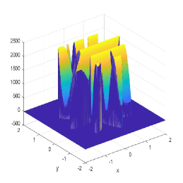
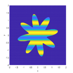
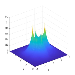
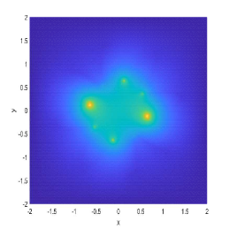
Figure 9. Performance of the proposed hybrid FDM in case of Example 3.2 : the numerical solution $(u_{h})_{i,j}$ (first and second panels) and $|(u_{h})_{i,j}-u(x_{i},y_{j})|$ (third and fourth panels) at all grid points $(x_{i},y_{j})$ on $\overline{\Omega}=[-2,2]^{2}$ with $h=2^{-7}$. Note that the second and fourth panels are just the 2D color map formats corresponding to the first and third panels, respectively.

3.2. Two numerical examples with unknown $u$

Example 3.3.

Let $\Omega=(-3/2,3/2)^{2}$ and the functions in (1.1) are given by

$$\Gamma=\{(x,y):\ x(\theta)=\cos(\theta),\ y(\theta)=1/2\sin(\theta)\},$$

$$\Omega_{+}=\{(x,y)\in\Omega:x^{2}(\theta)+4y^{2}(\theta)>1\},\qquad a_{+}=2+\sin(x+y),\qquad f_{+}=\cos(\pi x)\cos(\pi y),$$

$$\Omega_{-}=\{(x,y)\in\Omega:x^{2}(\theta)+4y^{2}(\theta)<1\},\qquad a_{-}=10^{4}(2+\sin(x+y)),\qquad f_{-}=\sin(\pi(x-y)),$$

$$g=\frac{|x^{\prime}(\theta)y^{\prime\prime}(\theta)-x^{\prime\prime}(\theta)y^{\prime}(\theta)|}{((x^{\prime}(\theta))^{2}+(y^{\prime}(\theta))^{2})^{3/2}}-1,\qquad g_{\Gamma}=\frac{|x^{\prime}(\theta)y^{\prime\prime}(\theta)-x^{\prime\prime}(\theta)y^{\prime}(\theta)|}{((x^{\prime}(\theta))^{2}+(y^{\prime}(\theta))^{2})^{3/2}},\quad\mbox{for}\quad\theta\in[0,2\pi),$$

$$\tfrac{\partial u}{\partial\vec{n}}+(\cos(y)+2)u=\sin(2\pi y)\text{ on }\Gamma_{1},\qquad u=0\text{ on }\Gamma_{2},$$

$$\tfrac{\partial u}{\partial\vec{n}}+(\sin(x)+2)u=\cos(\pi x)\text{ on }\Gamma_{3},\qquad u=0\text{ on }\Gamma_{4}.$$

Note that the exact solution $u$ is unknown in this example, and $\frac{|x^{\prime}(\theta)y^{\prime\prime}(\theta)-x^{\prime\prime}(\theta)y^{\prime}(\theta)|}{((x^{\prime}(\theta))^{2}+(y^{\prime}(\theta))^{2})^{3/2}}$ is just the curvature of $\Gamma$ at the point $(x(\theta),y(\theta))\in\Gamma$. Therefore, the data $g,g_{\Gamma}$ on $\Gamma$ are functions depending only on the curvature of the interface $\Gamma$. $\|u_{h}\|_{\infty}=1.7822$ with $J=10$. The numerical results are presented in Tables 1 and 2 and Fig. 10.

Figure 10. Performance of the proposed hybrid FDM in case of Example 3.3: the numerical solution $(u_{h})_{i,j}$ (first and second panels) at all grid points $(x_{i},y_{j})$ on $\overline{\Omega}=[-3/2,3/2]^{2}$ with $h=\tfrac{3}{2^{10}}$, and $|(u_{h})_{i,j}-(u_{h/2})_{2i,2j}|$ (third and fourth panels) at all grid points $(x_{i},y_{j})$ on $\overline{\Omega}=[-3/2,3/2]^{2}$ with $h=\tfrac{3}{2^{9}}$. Note that the second and fourth panels are just the 2D color map formats corresponding to the first and third panels, respectively.

Example 3.4.

Let $\Omega=(-2,2)^{2}$ and the functions in (1.1) are given by

$$\Gamma=\{(x,y):\ x(\theta)=(\pi/3+0.4\sin(10\theta))\cos(\theta),\ y(\theta)=(\pi/3+0.4\sin(10\theta))\sin(\theta)\},$$

$$\Omega_{+}=\{(x,y)\in\Omega:x^{2}(\theta)+y^{2}(\theta)>(\pi/3+0.4\sin(10\theta))^{2}\},\qquad a_{+}=10^{3}(2+\cos(x)\cos(y)),$$

$$\Omega_{-}=\{(x,y)\in\Omega:x^{2}(\theta)+y^{2}(\theta)<(\pi/3+0.4\sin(10\theta))^{2}\},\qquad a_{-}=2+\cos(x)\cos(y),$$

$$f_{+}=\sin(\pi x)\sin(\pi y),\qquad f_{-}=\cos(\pi x)\cos(\pi y),$$

$$g=-\sin(\theta)-1,\qquad g_{\Gamma}=\cos(\theta),\qquad\mbox{for}\qquad\theta\in[0,2\pi),\qquad u=0\text{ on }\partial\Omega.$$

Note that the exact solution $u$ is unknown in this example and $\|u_{h}\|_{\infty}=1.9992$ with $J=10$. The numerical results are presented in Tables 1 and 2 and Fig. 11.

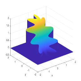
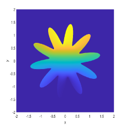
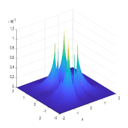
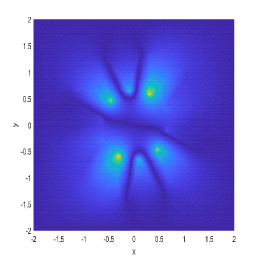
Figure 11. Performance of the proposed hybrid FDM in case of Example 3.4: the numerical solution $(u_{h})_{i,j}$ (first and second panels) at all grid points $(x_{i},y_{j})$ on $\overline{\Omega}=[-2,2]^{2}$ with $h=2^{-8}$, and $|(u_{h})_{i,j}-(u_{h/2})_{2i,2j}|$ (third and fourth panels) at all grid points $(x_{i},y_{j})$ on $\overline{\Omega}=[-2,2]^{2}$ with $h=2^{-7}$. Note that the second and fourth panels are just the 2D color map formats corresponding to the first and third panels, respectively.

Remark 3.5.

We extended the method proposed in this paper to the Helmholtz interface problem $\Delta u+{\textsf{k}}^{2}u=f$ in $\Omega\setminus\Gamma$ with $\left[u\right]=g$ and $\left[\nabla u\cdot\vec{n}\right]=g_{\Gamma}$ on $\Gamma$ in [6]. More precisely, [6] derived a fifth-order 9-point compact FDM for piecewise constant wavenumbers, and a sixth-order 9-point compact FDM with reduced pollution effect for constant wavenumbers. We also provided the results of four numerical experiments that confirm the order of convergence: Examples 3.5 and 3.6 consider constant wavenumbers and Examples 3.7 and 3.8 consider discontinuous piecewise constant wavenumbers.

Remark 3.6.

We consider complex interface curves $\Gamma$ in Examples 3.2 and 3.4 (an eight-star interface and a ten-star interface). From Fig. 12, we observe that when the $J$ is small (i.e., the mesh size $h$ is coarse), the interface curves $\Gamma$ have large curvatures within some 13-point stencils. So the errors observed in Examples 3.2 and 3.4 are large when $J$ is small (see Table 1). Motivated by the pollution minimization strategy in [6], we plan to propose a new technique to tackle this issue in our future work.

Figure 12. The 13-point scheme at the irregular point $(x_{i},y_{j})=(0.375,-0.625)$ for Example 3.2 with $J=5$ (left) and the 13-point scheme at the irregular point $(x_{i},y_{j})=(0.5,-0.75)$ for Example 3.4 with $J=4$ (right).

4. Conclusion

Regarding the proposed sixth-order compact FDM at regular points:

• To our best knowledge, thus far in the literature there were no schemes for solving the elliptic equation $-\nabla\cdot(a\nabla u)=f$ with a scalar variable coefficient $a>0$, that could achieve fourth and higher order consistency and the M-matrix property for any $h>0$. We prove the existence of a 9-point compact FDM with the sixth-order consistency, satisfying the M-matrix property for any $h>0$ without any mesh constraints and we explicitly construct such a scheme.

• We also derive the $6$-point/$4$-point compact FDMs with the sixth-order consistency and satisfying the M-matrix property for any $h>0$ at the side/corner boundary points for any mixed boundary conditions under the proposed necessary condition of the boundary functions $\alpha,\beta$.

• The matrices ($A_{d}$ with $d=0,\dots,6$ or 7, see (2.27)–(2.28), (A.73)-(A.74) and (A.100)–(A.101)) of linear systems to derive the above FDMs are constant matrices. High order (partial) derivatives of $a,\alpha,\beta$ only appear on the right hand side of linear systems.

Regarding the proposed fifth-order $13$-point FDM at irregular points:

• We propose a 13-point FDM with the fifth-order consistency, and our numerical experiments confirm the sixth-order convergence in the $l_{\infty}$ norm of the combined hybrid scheme.

• To obtain the stencil coefficients of the 13-point FDM with the fifth-order consistency, we explicitly derive a recursive solver to decompose the original linear system into six smaller ones. This significantly reduces the computational cost and make the implementation efficient.

• The matrices ($A_{d}$ with $d=0,\dots,5$, see (2.41)–(2.44)) of linear systems to obtain the stencil coefficients of the above FDM only depend on $a_{\pm}^{(0,0)}$, the first derivative of $\Gamma$ and $(v_{0},w_{0})$ in (2.30). High order (partial) derivatives of $a_{\pm}$ and $\Gamma$ only appear on the right hand side of linear systems.

Finally, our proposed FDMs are independent of the choice of local parametric equations (or the level set functions) of $\Gamma$ near the base point and can handle the jump functions $g,g_{\Gamma}$ along $\Gamma$ which only depend on the geometry (such as curvature) of $\Gamma$. Moreover, we only use function values to numerically approximate (without losing accuracy) high order (partial) derivatives of the coefficient $a$, the source term $f$, the interface curve $\Gamma$, the two jump functions on $\Gamma$, and the functions on $\partial\Omega$.

Appendix A Proofs of Theorems 2.1, 2.2 and 2.3 and FDMs at boundary grid points

A.1. Proofs of Theorems 2.1, 2.2 and 2.3

We now prove Theorems 2.1, 2.2 and 2.3 stated in Section 2.

Proof of Theorem 2.1.

Applying the definition of $\mathcal{L}_{h}$ in (2.24) to the exact solution $u$, we have

$$\begin{split}&h^{-2}\mathcal{L}_{h}u=h^{-2}\sum_{k=-1}^{1}\sum_{\ell=-1}^{1}C_{k,\ell}u(x_{i}+kh,y_{j}+\ell h),\end{split}$$

where the stencil coefficients $C_{k,\ell}$ are defined in (2.21), i.e., $C_{k,\ell}:=\sum_{p=0}^{M+1}c_{k,\ell,p}h^{p}$. Using the established identity (2.12) with the particular base point $(x_{i}^{*},y^{*}_{j}):=(x_{i},y_{j})$, we have

$$\begin{split}&h^{-2}\mathcal{L}_{h}u=h^{-2}\sum_{(m,n)\in\Lambda_{M+1}^{1}}u^{(m,n)}I_{m,n}+\sum_{(m,n)\in\Lambda_{M-1}}f^{(m,n)}J_{m,n}+\mathcal{O}(h^{M}),\end{split}$$ (A.1)

where

$$\begin{split}I_{m,n}=\sum_{k=-1}^{1}\sum_{\ell=-1}^{1}C_{k,\ell}G_{M+1,m,n}(kh,\ell h),\qquad J_{m,n}=h^{-2}\sum_{k=-1}^{1}\sum_{\ell=-1}^{1}C_{k,\ell}H_{M+1,m,n}(kh,\ell h).\end{split}$$ (A.2)

Then (A.1) and (2.24) yield $h^{-2}\mathcal{L}_{h}(u-u_{h})=\mathcal{O}(h^{M})$, if $I_{m,n}$ in (A.2) satisfies

$$\sum_{k=-1}^{1}\sum_{\ell=-1}^{1}C_{k,\ell}G_{M+1,m,n}(kh,\ell h)=\mathcal{O}(h^{M+2})\quad\mbox{for all}\quad(m,n)\in\Lambda_{M+1}^{1}.$$ (A.3)

By the symbolic calculation, (A.3) has a nontrivial solution $\{C_{k,\ell}\}_{k,\ell=-1,0,1}$ if and only if $M\leq 6$. We now derive (2.25) and prove items (i) and (ii) in Theorem 2.1. First, (A.3) with $m=n=0$, (2.15), and (2.21) lead to

$$\sum\limits_{k=-1}^{1}\sum\limits_{\ell=-1}^{1}c_{k,\ell,p}=0,\quad\mbox{for}\quad p=0,\dots,M+1.$$ (A.4)

So we proved the item (i) in Theorem 2.1. By (2.21) and (2.13), (A.3) becomes

$$\begin{split}&\sum_{k=-1}^{1}\sum_{\ell=-1}^{1}\sum_{p=0}^{M+1}c_{k,\ell,p}h^{p}\Big{(}G_{m,n}(kh,\ell h)+\sum_{(p,q)\in\Lambda_{M+1}^{2}\setminus\Lambda_{m+n}^{2}}\frac{a^{u}_{p,q,m,n}}{p!q!}(kh)^{p}(\ell h)^{q}\Big{)}\\ &=\mathcal{O}(h^{M+2}),\qquad\text{for all }(m,n)\in\Lambda_{M+1}^{1},\end{split}$$ (A.5)

i.e.,

$$\begin{split}&\sum_{k=-1}^{1}\sum_{\ell=-1}^{1}\sum_{p=0}^{M+1}c_{k,\ell,p}h^{p}G_{m,n}(kh,\ell h)\\ &+\sum_{k=-1}^{1}\sum_{\ell=-1}^{1}\sum_{s=0}^{M+1}c_{k,\ell,s}h^{s}\sum_{(p,q)\in\Lambda_{M+1}^{2}\setminus\Lambda_{m+n}^{2}}\frac{a^{u}_{p,q,m,n}}{p!q!}k^{p}\ell^{q}h^{p+q}=\mathcal{O}(h^{M+2}),\quad\text{for all }(m,n)\in\Lambda_{M+1}^{1}.\end{split}$$ (A.6)

Since $(p,q)\in\Lambda_{M+1}^{2}\setminus\Lambda_{m+n}^{2}$ implies $p+q>m+n$, we have that the degree of $h$ of $k^{p}\ell^{q}h^{p+q}$ must be greater than $m+n$, if $k^{p}\ell^{q}h^{p+q}\neq 0$. By (2.14), the degree of $h$ of $G_{m,n}(kh,\ell h)$ is $m+n$, if $G_{m,n}(kh,\ell h)\neq 0$. Consider non-zero terms $h^{m+n+d}$ in (A.6) with $0\leq d\leq M+1-m-n$, we deduce

$$\begin{split}&\sum_{k=-1}^{1}\sum_{\ell=-1}^{1}c_{k,\ell,d}h^{d}G_{m,n}(kh,\ell h)+\sum_{k=-1}^{1}\sum_{\ell=-1}^{1}\sum_{s=0}^{M+1}c_{k,\ell,s}h^{s}\sum_{\begin{subarray}{c}(p,q)\in\Lambda_{M+1}^{2}\setminus\Lambda_{m+n}^{2}\\ p+q=m+n+d-s\end{subarray}}\frac{a^{u}_{p,q,m,n}}{p!q!}k^{p}\ell^{q}h^{p+q}\\ &=\mathcal{O}(h^{M+2}),\quad\mbox{ for all }0\leq d\leq M+1-m-n\mbox{ and }(m,n)\in\Lambda_{M+1}^{1}.\end{split}$$ (A.7)

By (2.4)–(2.14), we can say that (A.7) is equivalent to

$$\begin{split}&\sum_{k=-1}^{1}\sum_{\ell=-1}^{1}c_{k,\ell,d}G_{m,n}(k,\ell)+\sum_{k=-1}^{1}\sum_{\ell=-1}^{1}\sum_{s=0}^{M+1}c_{k,\ell,s}\sum_{\begin{subarray}{c}(p,q)\in\Lambda_{M+1}^{2}\setminus\Lambda_{m+n}^{2}\\ p+q=m+n+d-s\end{subarray}}\frac{a^{u}_{p,q,m,n}}{p!q!}k^{p}\ell^{q}=0,\\ &\mbox{ for all }0\leq d\leq M+1-m-n\mbox{ and }(m,n)\in\Lambda_{M+1}^{1}.\end{split}$$ (A.8)

Note that $(p,q)\in\Lambda_{M+1}^{2}\setminus\Lambda_{m+n}^{2}$ results in $m+n+1\leq p+q\leq M+1$. By $p+q=m+n+d-s$, $1\leq d-s\leq M+1-m-n$, so $s\leq d-1$. By the definition of $\Lambda_{M+1}^{1}$ in (2.5), $0\leq d\leq M+1-m-n$ and $(m,n)\in\Lambda_{M+1}^{1}$ can be equivalently rewritten as $(m,n)\in\Lambda_{M+1-d}^{1}$ and $0\leq d\leq M+1$. So (A.8) is equivalent to

$$\begin{split}&\sum_{k=-1}^{1}\sum_{\ell=-1}^{1}c_{k,\ell,d}G_{m,n}(k,\ell)+\sum_{k=-1}^{1}\sum_{\ell=-1}^{1}\sum_{s=0}^{d-1}c_{k,\ell,s}A^{u}_{k,\ell,m,n,s}=0,\\ &\mbox{with}\quad A^{u}_{k,\ell,m,n,s}:=\sum_{\begin{subarray}{c}(p,q)\in\Lambda_{M+1}^{2}\setminus\Lambda_{m+n}^{2}\\ p+q=m+n+d-s\end{subarray}}\frac{a^{u}_{p,q,m,n}}{p!q!}k^{p}\ell^{q}\qquad\quad\mbox{ for all }(m,n)\in\Lambda_{M+1-d}^{1},\end{split}$$ (A.9)

for all $d=0,\ldots,M+1$. By (A.5)–(A.9), we can say that (A.3) is equivalent to (A.9). Note that $\sum_{s=0}^{d-1}$ in (A.9) is empty for $d=0$. Now (2.25) in Theorem 2.1 can be seen from (A.9) with $M=6$.

The system of linear equations in (A.9) can be represented in the following matrix form:

$$\begin{pmatrix}A_{0}&\textbf{0}&\textbf{0}&\cdots&\textbf{0}&\textbf{0}\\ B_{1,0}&A_{1}&\textbf{0}&\cdots&\textbf{0}&\textbf{0}\\ B_{2,0}&B_{2,1}&A_{2}&\cdots&\textbf{0}&\textbf{0}\\ \vdots&\vdots&\vdots&\ddots&\vdots&\vdots\\ B_{M,0}&B_{M,1}&B_{M,2}&\cdots&A_{M}&\textbf{0}\\ \textbf{0}&\textbf{0}&\textbf{0}&\cdots&\textbf{0}&A_{M+1}\\ \end{pmatrix}\begin{pmatrix}C_{0}\\ C_{1}\\ C_{2}\\ \vdots\\ C_{M}\\ C_{M+1}\end{pmatrix}=\textbf{0},\text{ with }C_{d}={\tiny{\begin{pmatrix}c_{-1,-1,d}\\ c_{-1,0,d}\\ c_{-1,1,d}\\ c_{0,-1,d}\\ c_{0,0,d}\\ c_{0,1,d}\\ c_{1,-1,d}\\ c_{1,0,d}\\ c_{1,1,d}\end{pmatrix},}}$$ (A.10)

where $0\leq d\leq M+1$ and

$$\begin{split}&A_{d}:=[G_{m,n}(k,\ell)]_{(k,\ell)\in\{-1,0,1\}^{2},(m,n)\in\Lambda_{M+1-d}^{1}},\text{ with }0\leq d\leq M+1,\\ &B_{d,s}:=[A^{u}_{k,\ell,m,n,s}]_{(k,\ell)\in\{-1,0,1\}^{2},(m,n)\in\Lambda_{M+1-d}^{1}},\text{ with }1\leq d\leq M\text{ and }0\leq s\leq d-1.\end{split}$$

The $G_{m,n}(x,y)$ in (2.14) and $a^{u}_{p,q,m,n}$ in (2.6) imply that that every $A_{d}$ is a constant matrix, and every matrix $B_{d,s}$ only depends on $\{a^{(i,j)}:(i,j)\in\Lambda_{M}\}$. See (2.27) and (2.28) for $\{A_{d}:0\leq d\leq 7\}$ with $M=6$. Clearly, (A.3) is equivalent to (A.10). For the sake of brevity, let $\textsf{A}\textsf{C}=\textbf{0}$ represent the whole homogeneous linear system in (A.10) with $M=6$. Then $\text{rank}(\textsf{A})=48$ and the dimension of the solution C is 24 by the symbolic calculation. Clearly, (A.10) implies

$$A_{0}C_{0}=\textbf{0},\quad A_{d}C_{d}=b_{d}\text{ with }b_{d}:=-\sum_{s=0}^{d-1}B_{d,s}C_{s}\text{ for }1\leq d\leq M,\quad\mbox{and}\quad A_{M+1}C_{M+1}=0.$$ (A.11)

So $b_{d}$ depends on $\{C_{i}:0\leq i\leq d-1\}$ and $\{a^{(i,j)}:(i,j)\in\Lambda_{M}\}$ for $1\leq d\leq M$. By a direct calculation, we observe that the dimension of the solution of (A.11) is 24 for $M=6$ (see the following (A.13), (A.14), (A.16), (A.18), (A.21), (A.24) and (A.27)). Now we can say that (A.10) is equivalent to (A.11) for $M=6$, i.e., (A.3) is equivalent to (A.11) for $M=6$.

We now prove item (ii) in Theorem 2.1 by establishing the following (A.12)–(A.28). By $h>0$, the nontrivial $\{C_{k,\ell}\}_{k,\ell=-1,0,1}$ in (2.24) satisfies the sign condition (2.19) for any $h$ if it satisfies (2.22). By (A.11) with $M=6$, we have

$$A_{0}C_{0}=\textbf{0},\qquad A_{d}C_{d}=b_{d},\quad d=1,\dots,6,\qquad A_{7}C_{7}=0.$$ (A.12)

All solutions of $A_{0}C_{0}=\textbf{0}$ in (A.12) with $M=6$ can be represented as

$$\begin{split}&c_{0,0,0}=-20c_{1,1,0},\quad c_{-1,0,0}=c_{1,0,0}=c_{0,-1,0}=c_{0,1,0}=4c_{1,1,0},\quad c_{-1,-1,0}=c_{-1,1,0}=c_{1,-1,0}=c_{1,1,0},\end{split}$$ (A.13)

where $c_{1,1,0}$ is free parameter. Then $\{c_{k,\ell,0}\}_{k,\ell=-1,0,1}$ in (A.13) satisfies the condition in (2.22) if and only if $c_{1,1,0}<0$. All solutions of $A_{1}C_{1}=b_{1}$ in (A.12) with $M=6$ can be represented as

$$\begin{split}&c_{0,0,1}=-20c_{1,1,1}+r_{1,1},\quad c_{-1,0,1}=4c_{1,1,1}+r_{1,2},\quad c_{1,0,1}=4c_{1,1,1}+r_{1,3},\quad c_{0,-1,1}=4c_{1,1,1}+r_{1,4},\\ &c_{0,1,1}=4c_{1,1,1}+r_{1,5},\quad c_{-1,-1,1}=c_{1,1,1}+r_{1,6},\quad c_{-1,1,1}=c_{1,1,1}+r_{1,7},\quad c_{1,-1,1}=c_{1,1,1}+r_{1,8},\end{split}$$ (A.14)

where $c_{1,1,1}$ is the free parameter, $\{r_{1,p}\}_{p=1,\dots,8}$ only depends on $\{c_{k,\ell,0}\}_{k,\ell=-1,0,1}$ in (A.13) and $\{a^{(i,j)}:(i,j)\in\Lambda_{6}\}$ (a special (A.14) with explicit expressions is shown in (A.29)-(A.32)). Then $\{c_{k,\ell,1}\}_{k,\ell=-1,0,1}$ in (A.14) satisfies the condition in (2.22) if and only if

$$c_{1,1,1}\leq\min\{\tfrac{r_{1,1}}{20},\tfrac{-r_{1,2}}{4},\tfrac{-r_{1,3}}{4},\tfrac{-r_{1,4}}{4},\tfrac{-r_{1,5}}{4},-r_{1,6},-r_{1,7},-r_{1,8},0\}.$$ (A.15)

All solutions of $A_{d}C_{d}=b_{d}$ with $d=2,3$ in (A.12) with $M=6$ can be represented as

$$\begin{split}&c_{0,0,d}=-20c_{1,1,d}+r_{d,1},\quad c_{-1,0,d}=4c_{1,1,d}+r_{d,2},\quad c_{1,0,d}=4c_{1,1,d}+r_{d,3},\quad c_{0,-1,d}=4c_{1,1,d}+r_{d,4},\\ &c_{0,1,d}=4c_{1,1,d}+r_{d,5},\ c_{-1,-1,d}=c_{1,1,d}+r_{d,6},\ c_{-1,1,d}=c_{1,1,d}+r_{d,7},\ c_{1,-1,d}=c_{1,1,d}+r_{d,8},\ d=2,3,\end{split}$$ (A.16)

where $c_{1,1,d}$ with $d=2,3$ is the free parameter, $\{r_{d,p}\}_{p=1,\dots,8}$ only depends on $\{c_{k,\ell,s}\}_{k,\ell=-1,0,1}$ with $0\leq s\leq d-1$ in (A.13), (A.14), (A.16) and $\{a^{(i,j)}:(i,j)\in\Lambda_{6}\}$ for $d=2,3$ (a special (A.16) with explicit expressions is shown in (A.29)-(A.32)). Then $\{c_{k,\ell,d}\}_{k,\ell=-1,0,1}$ in (A.16) satisfies the condition in (2.22) if and only if

$$\begin{split}c_{1,1,d}\leq\min\{\tfrac{r_{d,1}}{20},\tfrac{-r_{d,2}}{4},\tfrac{-r_{d,3}}{4},\tfrac{-r_{d,4}}{4},\tfrac{-r_{d,5}}{4},-r_{d,6},-r_{d,7},-r_{d,8},0\},\quad d=2,3.\end{split}$$ (A.17)

All solutions of $A_{4}C_{4}=b_{4}$ in (A.12) with $M=6$ can be represented as

$$\begin{split}&c_{0,0,4}=-4c_{1,0,4}-4c_{1,1,4}+r_{4,1},\quad c_{-1,0,4}=c_{1,0,4}+r_{4,2},\quad c_{0,-1,4}=c_{1,0,4}+r_{4,3},\\ &c_{0,1,4}=c_{1,0,4}+r_{4,4},\quad c_{-1,-1,4}=c_{1,1,4}+r_{4,5},\quad c_{-1,1,4}=c_{1,1,4}+r_{4,6},\quad c_{1,-1,4}=c_{1,1,4}+r_{4,7},\end{split}$$ (A.18)

where $\{c_{1,0,4},c_{1,1,4}\}$ are the free parameters, $\{r_{4,p}\}_{p=1,\dots,7}$ only depends on $\{c_{k,\ell,s}\}_{k,\ell=-1,0,1}$ with $0\leq s\leq 3$ in (A.13), (A.14), (A.16) and $\{a^{(i,j)}:(i,j)\in\Lambda_{6}\}$ (a special (A.18) with explicit expressions is shown in (A.29)-(A.32)). Then $\{c_{k,\ell,4}\}_{k,\ell=-1,0,1}$ in (A.18) satisfies the condition (2.22) if and only if

$$\begin{split}&c_{1,0,4}+c_{1,1,4}\leq\tfrac{r_{4,1}}{4},\quad c_{1,0,4}\leq\min\{-r_{4,2},-r_{4,3},-r_{4,4},0\},\quad c_{1,1,4}\leq\min\{-r_{4,5},-r_{4,6},-r_{4,7},0\}.\end{split}$$ (A.19)

One non-empty interval of (A.19) is

$$\begin{split}c_{1,0,4}=c_{1,1,4},\qquad c_{1,1,4}\leq\min\{\tfrac{r_{4,1}}{8},-r_{4,2},-r_{4,3},-r_{4,4},-r_{4,5},-r_{4,6},-r_{4,7},0\}.\end{split}$$ (A.20)

All solutions of $A_{5}C_{5}=b_{5}$ in (A.12) with $M=6$ can be represented as

$$\begin{split}&c_{0,0,5}=-2c_{0,1,5}-2c_{1,0,5}-4c_{1,1,5}+r_{5,1},\\ &c_{-1,0,5}=2c_{0,1,5}-2c_{1,-1,5}-c_{1,0,5}+2c_{1,1,5}+r_{5,2},\quad c_{0,-1,5}=c_{0,1,5}-2c_{1,-1,5}+2c_{1,1,5}+r_{5,3},\\ &c_{-1,-1,5}=-c_{0,1,5}+2c_{1,-1,5}+c_{1,0,5}-c_{1,1,5}+r_{5,4},\quad c_{-1,1,5}=-c_{0,1,5}+c_{1,-1,5}+c_{1,0,5}+r_{5,5},\end{split}$$ (A.21)

where $\{c_{0,1,5},c_{1,-1,5},c_{1,0,5},c_{1,1,5}\}$ are the free parameters, $\{r_{5,p}\}_{p=1,\dots,5}$ only depends on $\{c_{k,\ell,s}\}_{k,\ell=-1,0,1}$ with $0\leq s\leq 4$ in (A.13), (A.14), (A.16), (A.18) and $\{a^{(i,j)}:(i,j)\in\Lambda_{6}\}$ (a special (A.21) with explicit expressions is shown in (A.29)-(A.32)). Then $\{c_{k,\ell,5}\}_{k,\ell=-1,0,1}$ in (A.21) satisfies the condition in (2.22) if and only if

$$\begin{split}&-2c_{0,1,5}-2c_{1,0,5}-4c_{1,1,5}+r_{5,1}\geq 0,\quad 2c_{0,1,5}-2c_{1,-1,5}-c_{1,0,5}+2c_{1,1,5}+r_{5,2}\leq 0,\\ &c_{0,1,5}-2c_{1,-1,5}+2c_{1,1,5}+r_{5,3}\leq 0,\quad-c_{0,1,5}+2c_{1,-1,5}+c_{1,0,5}-c_{1,1,5}+r_{5,4}\leq 0,\\ &-c_{0,1,5}+c_{1,-1,5}+c_{1,0,5}+r_{5,5}\leq 0,\quad c_{0,1,5}\leq 0,\quad c_{1,-1,5}\leq 0,\quad c_{1,0,5}\leq 0,\quad c_{1,1,5}\leq 0.\end{split}$$ (A.22)

One non-empty interval of (A.22) is

$$\begin{split}&c_{0,1,5}=c_{1,-1,5}=c_{1,0,5}=c_{1,1,5},\qquad c_{1,1,5}\leq\min\{\tfrac{r_{5,1}}{8},-r_{5,2},-r_{5,3},-r_{5,4},-r_{5,5},0\}.\end{split}$$ (A.23)

All solutions of $A_{6}C_{6}=b_{6}$ in (A.12) with $M=6$ can be represented as

$$\begin{split}&c_{-1,0,6}=-2c_{-1,1,6}-c_{0,0,6}-2c_{0,1,6}-c_{1,0,6}-2c_{1,1,6}+r_{6,1},\\ &c_{0,-1,6}=-c_{0,0,6}-c_{0,1,6}-2c_{1,-1,6}-2c_{1,0,6}-2c_{1,1,6}+r_{6,2},\\ &c_{-1,-1,6}=c_{-1,1,6}+c_{0,0,6}+2c_{0,1,6}+c_{1,-1,6}+2c_{1,0,6}+3c_{1,1,6}+r_{6,3},\end{split}$$ (A.24)

where $\{c_{-1,1,6},c_{0,0,6},c_{0,1,6},c_{1,-1,6},c_{1,0,6},c_{1,1,6}\}$ are the free parameters, $\{r_{6,p}\}_{p=1,2,3}$ only depends on $\{c_{k,\ell,s}\}_{k,\ell=-1,0,1}$ with $0\leq s\leq 5$ in (A.13), (A.14), (A.16), (A.18), (A.21) and $\{a^{(i,j)}:(i,j)\in\Lambda_{6}\}$ (a special (A.24) with explicit expressions is shown in (A.29)-(A.32)). Then $\{c_{k,\ell,6}\}_{k,\ell=-1,0,1}$ in (A.24) satisfies the condition in (2.22) if and only if

$$\begin{split}&-2c_{-1,1,6}-c_{0,0,6}-2c_{0,1,6}-c_{1,0,6}-2c_{1,1,6}+r_{6,1}\leq 0,\\ &-c_{0,0,6}-c_{0,1,6}-2c_{1,-1,6}-2c_{1,0,6}-2c_{1,1,6}+r_{6,2}\leq 0,\\ &c_{-1,1,6}+c_{0,0,6}+2c_{0,1,6}+c_{1,-1,6}+2c_{1,0,6}+3c_{1,1,6}+r_{6,3}\leq 0,\\ &c_{-1,1,6}\leq 0,\quad c_{0,0,6}\geq 0,\quad c_{0,1,6}\leq 0,\quad c_{1,-1,6}\leq 0,\quad c_{1,0,6}\leq 0,\quad c_{1,1,6}\leq 0.\end{split}$$ (A.25)

One non-empty interval of (A.25) is

$$\begin{split}&c_{-1,1,6}=c_{0,1,6}=c_{1,-1,6}=c_{1,0,6}=c_{1,1,6},\quad c_{0,0,6}=-8c_{1,1,6},\quad c_{1,1,6}\leq\min\{-r_{6,1},-r_{6,2},-r_{6,3},0\}.\end{split}$$ (A.26)

All solutions of $A_{7}C_{7}=0$ in (A.12) with $M=6$ are

$$c_{0,0,7}=-c_{-1,0,7}-c_{1,0,7}-c_{0,-1,7}-c_{0,1,7}-c_{-1,-1,7}-c_{-1,1,7}-c_{1,-1,7}-c_{1,1,7},$$ (A.27)

where $\{c_{-1,0,7},c_{1,0,7},c_{0,-1,7},c_{0,1,7},c_{-1,-1,7},c_{-1,1,7},c_{1,-1,7},c_{1,1,7}\}$ are free parameters. Then $\{c_{k,\ell,7}\}_{k,\ell=-1,0,1}$ in (A.27) satisfies the condition in (2.22) if and only if

$$\begin{split}&c_{0,0,7}=-c_{-1,0,7}-c_{1,0,7}-c_{0,-1,7}-c_{0,1,7}-c_{-1,-1,7}-c_{-1,1,7}-c_{1,-1,7}-c_{1,1,7}\geq 0,\quad c_{1,1,7}\leq 0,\\ &c_{-1,0,7}\leq 0,\quad c_{1,0,7}\leq 0,\quad c_{0,-1,7}\leq 0,\quad c_{0,1,7}\leq 0,\quad c_{-1,-1,7}\leq 0,\quad c_{-1,1,7}\leq 0,\quad c_{1,-1,7}\leq 0.\end{split}$$ (A.28)

One non-empty interval of (A.28) is $c_{k,\ell,7}=0$ for $k,\ell\in\{-1,0,1\}$. By the symbolic calculation, all $r_{d,p}$ $\neq\pm\infty$ in (A.15)–(A.26) by $a\neq 0$ in $\Omega$. By (A.12)–(A.28), we proved the item (ii) in Theorem 2.1. ∎

The explicit expressions for a particular $\{C_{k,\ell}\}$ in Theorem 2.1: Let $a(x,y)$ be a linear function (i.e., all $a^{(m,n)}$ are 0 for $m+n\geq 2$), $r_{1}=a^{(1,0)}/a^{(0,0)}$ and $r_{2}=a^{(0,1)}/a^{(0,0)}$. Then the explicit expressions of $C_{k,\ell}:=\sum_{p=0}^{7}c_{k,\ell,p}h^{p}$ in (2.24) with the sixth-order consistency and satisfying the sign condition (2.19) and the sum condition (2.20) for any mesh size $h$ are defined in the following (A.29)–(A.32) (we highlight the free parameters using the color red or blue to increase the visibility):

$$\begin{split}&c_{0,0,0}=20,\ c_{-1,0,0}=c_{1,0,0}=c_{0,-1,0}=c_{0,1,0}=-4,\ c_{-1,-1,0}=c_{-1,1,0}=c_{1,-1,0}=c_{1,1,0}=-1,\\ &c_{0,0,d}=-20c_{d}+r_{d,1},\quad c_{-1,0,d}=4c_{d}+r_{d,2},\quad c_{1,0,d}=4c_{d}+r_{d,3},\quad c_{0,-1,d}=4c_{d}+r_{d,4},\\ &c_{0,1,d}=4c_{d}+r_{d,5},\quad c_{-1,-1,d}=c_{d}+r_{d,6},\quad c_{-1,1,d}=c_{d}+r_{d,7},\quad c_{1,-1,d}=c_{d}+r_{d,8},\\ &c_{1,1,d}=c_{d},\quad{\color[rgb]{1,0,0}c_{d}}=\min\{r_{d,1}/20,-r_{d,2}/4,-r_{d,3}/4,-r_{d,4}/4,-r_{d,5}/4,-r_{d,6},-r_{d,7},-r_{d,8},0\},\end{split}$$ (A.29)

for $d=1,2,3$, where

$$\begin{split}&r_{1,1}=-10(r_{1}+r_{2}),\quad r_{1,2}=4r_{1}+2r_{2},\quad r_{1,3}=2r_{2},\quad r_{1,4}=2r_{1}+4r_{2},\\ &r_{1,5}=2r_{1},\quad r_{1,6}=r_{1}+r_{2},\quad r_{1,7}=r_{1},\quad r_{1,8}=r_{2},\\ &r_{2,p}=-r_{1,p}{\color[rgb]{0,0,1}c_{1}}+r_{p+2},\quad r_{3,p}=-r_{p+2}{\color[rgb]{0,0,1}c_{1}}-r_{1,p}{\color[rgb]{0,0,1}c_{2}}+r_{10+p},\quad\text{for}\quad p=1,\dots,8,\end{split}$$

and

$$\begin{split}&r_{3}=29/5(r_{1}^{2}+r_{2}^{2})+15r_{1}r_{2},\quad r_{4}=-(39r_{1}^{2}+29r_{2}^{2})/20-4r_{1}r_{2},\quad r_{5}=(r_{1}^{2}-29r_{2}^{2})/20-2r_{1}r_{2},\\ &r_{6}=-(39r_{2}^{2}+29r_{1}^{2})/20-4r_{1}r_{2},\quad r_{7}=(r_{2}^{2}-29r_{1}^{2})/20-2r_{1}r_{2},\quad r_{8}=-(r_{1}+r_{2})^{2}/2,\\ &r_{9}=-r_{1}(2r_{2}+r_{1})/2,\quad r_{10}=-r_{2}(2r_{1}+r_{2})/2,\quad r_{11}=-127/30(r_{1}^{3}+r_{2}^{3})-251/15(r_{1}^{2}r_{2}+r_{1}r_{2}^{2}),\\ &r_{12}=(119r_{2}^{3}+569r_{1}^{2}r_{2})/120+(49r_{1}r_{2}^{2}+19r_{1}^{3})/12,\quad r_{13}=(119r_{2}^{3}+209r_{1}^{2}r_{2})/120+(29r_{1}r_{2}^{2}-r_{1}^{3})/10,\\ &r_{14}=(119r_{1}^{3}+569r_{1}r_{2}^{2})/120+(49r_{1}^{2}r_{2}+19r_{2}^{3})/12,\quad r_{15}=(119r_{1}^{3}+209r_{1}r_{2}^{2})/120+(29r_{1}^{2}r_{2}-r_{2}^{3})/10,\\ &r_{16}=23/60(r_{1}^{3}+r_{2}^{3})+83/60(r_{1}^{2}r_{2}+r_{1}r_{2}^{2}),\ r_{17}=(23r_{1}^{3}+53r_{1}r_{2}^{2})/60+r_{1}^{2}r_{2},\ r_{18}=(23r_{2}^{3}+53r_{1}^{2}r_{2})/60+r_{1}r_{2}^{2}.\end{split}$$

$$\begin{split}&c_{0,0,4}=-8c_{4}+r_{4,1},\quad c_{-1,0,4}=c_{4}+r_{4,2},\quad c_{0,-1,4}=c_{4}+r_{4,3},\quad c_{0,1,4}=c_{4}+r_{4,4},\\ &c_{-1,-1,4}=c_{4}+r_{4,5},\quad c_{-1,1,4}=c_{4}+r_{4,6},\quad c_{1,-1,4}=c_{4}+r_{4,7},\quad c_{1,0,4}=c_{1,1,4}=c_{4},\\ &{\color[rgb]{1,0,0}c_{4}}=\min\{r_{4,1}/8,-r_{4,2},-r_{4,3},-r_{4,4},-r_{4,5},-r_{4,6},-r_{4,7},0\},\end{split}$$ (A.30)

where

$$\begin{split}r_{4,1}=&(139r_{1}^{3}+293r_{1}^{2}r_{2}+154r_{1}r_{2}^{2}+8r_{2}^{3})/30{\color[rgb]{0,0,1}c_{1}}-(6r_{1}^{2}+7r_{1}r_{2}){\color[rgb]{0,0,1}c_{2}}+2(5r_{1}+r_{2}){\color[rgb]{0,0,1}c_{3}}+(413r_{1}^{4}-23r_{2}^{4})/120+23/2r_{1}^{2}r_{2}^{2}\\ &+(34r_{1}^{3}r_{2}+13r_{1}r_{2}^{3})/3,\\ r_{4,2}=&(-(101r_{1}^{3}+71r_{1}r_{2}^{2})/60-3r_{1}^{2}r_{2}){\color[rgb]{0,0,1}c_{1}}+2r_{1}(r_{1}+r_{2}){\color[rgb]{0,0,1}c_{2}}-4r_{1}{\color[rgb]{0,0,1}c_{3}}-(133r_{1}^{4}+433r_{1}^{3}r_{2}+403r_{1}^{2}r_{2}^{2}+103r_{1}r_{2}^{3})/120,\\ r_{4,3}=&(-131r_{1}^{3}-281r_{1}^{2}r_{2}-221r_{1}r_{2}^{2}-71r_{2}^{3})/120{\color[rgb]{0,0,1}c_{1}}+(3r_{1}+r_{2})(r_{1}+r_{2})/2{\color[rgb]{0,0,1}c_{2}}-2(r_{1}+r_{2}){\color[rgb]{0,0,1}c_{3}}-1/5r_{2}^{4}-(109r_{1}^{4}\\ &+403r_{1}^{2}r_{2}^{2}+223r_{1}r_{2}^{3}+313r_{1}^{3}r_{2})/120,\\ r_{4,4}=&(131(r_{2}^{3}-r_{1}^{3})+139(r_{1}r_{2}^{2}-r_{1}^{2}r_{2}))/120{\color[rgb]{0,0,1}c_{1}}+3/2(r_{1}^{2}-r_{2}^{2}){\color[rgb]{0,0,1}c_{2}}+2(r_{2}-r_{1}){\color[rgb]{0,0,1}c_{3}}+109/120(r_{2}^{4}-r_{1}^{4})+7/4(r_{1}r_{2}^{3}-r_{1}^{3}r_{2}),\\ r_{4,5}=&-23/60(r_{1}^{2}+60/23r_{1}r_{2}+r_{2}^{2})(r_{1}+r_{2}){\color[rgb]{0,0,1}c_{1}}+(r_{1}+r_{2})^{2}/2{\color[rgb]{0,0,1}c_{2}}-(r_{1}+r_{2}){\color[rgb]{0,0,1}c_{3}}-31/120(r_{1}^{2}+90/31r_{1}r_{2}+r_{2}^{2})(r_{1}+r_{2})^{2},\\ r_{4,6}=&(-(53r_{1}r_{2}^{2}+23r_{1}^{3})/60-r_{1}^{2}r_{2}){\color[rgb]{0,0,1}c_{1}}+(r_{1}+2r_{2})r_{1}/2{\color[rgb]{0,0,1}c_{2}}-r_{1}{\color[rgb]{0,0,1}c_{3}}-31/120r_{1}^{4}-13/10r_{1}^{3}r_{2}-83/60r_{1}^{2}r_{2}^{2}-4/5r_{1}r_{2}^{3},\\ r_{4,7}=&(-(53r_{1}^{2}r_{2}+23r_{2}^{3})/60-r_{1}r_{2}^{2}){\color[rgb]{0,0,1}c_{1}}+(r_{2}+2r_{1})r_{2}/2{\color[rgb]{0,0,1}c_{2}}-r_{2}{\color[rgb]{0,0,1}c_{3}}-31/120r_{2}^{4}-13/10r_{1}r_{2}^{3}-83/60r_{1}^{2}r_{2}^{2}-4/5r_{1}^{3}r_{2}.\end{split}$$

$$\begin{split}&c_{0,0,5}=-8c_{5}+r_{5,1},\quad c_{-1,0,5}=c_{5}+r_{5,2},\quad c_{0,-1,5}=c_{5}+r_{5,3},\quad c_{-1,-1,5}=c_{5}+r_{5,4},\\ &c_{-1,1,5}=c_{5}+r_{5,5},\quad c_{0,1,5}=c_{1,-1,5}=c_{1,0,5}=c_{1,1,5}=c_{5},\\ &{\color[rgb]{1,0,0}c_{5}}=\min\{r_{5,1}/8,-r_{5,2},-r_{5,3},-r_{5,4},-r_{5,5},0\},\end{split}$$ (A.31)

where

$$\begin{split}r_{5,1}=&(-207r_{1}^{4}-743r_{1}^{3}r_{2}-823r_{1}^{2}r_{2}^{2}-473r_{1}r_{2}^{3}-76r_{2}^{4})/120{\color[rgb]{0,0,1}c_{1}}+(5/2r_{1}^{3}+11/2r_{1}^{2}r_{2}+4r_{1}r_{2}^{2}+r_{2}^{3}){\color[rgb]{0,0,1}c_{2}}-(3r_{1}^{2}+5r_{1}r_{2}+r_{2}^{2}){\color[rgb]{0,0,1}c_{3}}\\ &+3(r_{1}+r_{2}){\color[rgb]{0,0,1}c_{4}}-73/48r_{1}^{5}-749/120r_{1}^{4}r_{2}-521/48r_{1}^{3}r_{2}^{2}-437/48r_{1}^{2}r_{2}^{3}-43/12r_{1}r_{2}^{4}-49/80r_{2}^{5},\\ r_{5,2}=&(217r_{1}^{3}r_{2}-85r_{1}^{4}+526r_{1}^{2}r_{2}^{2}+487r_{1}r_{2}^{3}+161r_{2}^{4})/120{\color[rgb]{0,0,1}c_{1}}+(r_{1}^{3}/2-3/2r_{2}^{3}-7/2r_{1}r_{2}^{2}-5/2r_{1}^{2}r_{2}){\color[rgb]{0,0,1}c_{2}}+(2r_{2}^{2}-r_{1}^{2}+4r_{1}r_{2}){\color[rgb]{0,0,1}c_{3}}\\ &-3r_{2}{\color[rgb]{0,0,1}c_{4}}+31/30r_{2}^{5}+241/60r_{1}r_{2}^{4}+869/120r_{1}^{2}r_{2}^{3}+1133/240r_{1}^{3}r_{2}^{2}+23/24r_{1}^{4}r_{2}-101/240r_{1}^{5},\\ r_{5,3}=&(76r_{2}^{4}+397r_{1}r_{2}^{3}+526r_{1}^{2}r_{2}^{2}+307r_{1}^{3}r_{2})/120{\color[rgb]{0,0,1}c_{1}}-3r_{2}(r_{1}^{2}+r_{1}r_{2}+1/3r_{2}^{2}){\color[rgb]{0,0,1}c_{2}}+r_{2}(4r_{1}+r_{2}){\color[rgb]{0,0,1}c_{3}}-3r_{2}{\color[rgb]{0,0,1}c_{4}}+49/80r_{2}^{5}\\ &+713/240r_{1}r_{2}^{4}+397/60r_{1}^{2}r_{2}^{3}+1283/240r_{1}^{3}r_{2}^{2}+481/240r_{1}^{4}r_{2},\\ r_{5,4}=&(292r_{1}^{4}+119r_{1}^{3}r_{2}-319r_{1}^{2}r_{2}^{2}-511r_{1}r_{2}^{3}-161r_{2}^{4})/240{\color[rgb]{0,0,1}c_{1}}+(r_{1}^{2}r_{2}/4-3/2r_{1}^{3}+3/2r_{1}r_{2}^{2}+3/4r_{2}^{3}){\color[rgb]{0,0,1}c_{2}}+(2r_{1}^{2}-2r_{1}r_{2}\\ &-r_{2}^{2}){\color[rgb]{0,0,1}c_{3}}+3/2(r_{2}-r_{1}){\color[rgb]{0,0,1}c_{4}}+233/240r_{1}^{5}+671/480r_{1}^{4}r_{2}-77/480r_{1}^{3}r_{2}^{2}-469/160r_{1}^{2}r_{2}^{3}-311/160r_{1}r_{2}^{4}-31/60r_{2}^{5},\\ r_{5,5}=&(292r_{1}^{4}+319r_{1}^{3}r_{2}-139r_{1}^{2}r_{2}^{2}-311r_{1}r_{2}^{3}-161r_{2}^{4})/240{\color[rgb]{0,0,1}c_{1}}+(r_{1}r_{2}^{2}-3/2r_{1}^{3}-r_{1}^{2}r_{2}/4+3/4r_{2}^{3}){\color[rgb]{0,0,1}c_{2}}+(r_{2}+2r_{1})(r_{1}\\ &-r_{2}){\color[rgb]{0,0,1}c_{3}}+3/2(r_{2}-r_{1}){\color[rgb]{0,0,1}c_{4}}+233/240r_{1}^{5}+301/160r_{1}^{4}r_{2}+91/96r_{1}^{3}r_{2}^{2}-175/96r_{1}^{2}r_{2}^{3}-701/480r_{1}r_{2}^{4}-31/60r_{2}^{5}.\end{split}$$

$$\begin{split}&c_{0,0,6}=-8c_{6},\quad c_{-1,0,6}=c_{6}+r_{6,1},\quad c_{0,-1,6}=c_{6}+r_{6,2},\quad c_{-1,-1,6}=c_{6}+r_{6,3},\\ &c_{-1,1,6}=c_{0,1,6}=c_{1,-1,6}=c_{1,0,6}=c_{1,1,6}=c_{6},\quad{\color[rgb]{1,0,0}c_{6}}=\min\{-r_{6,1},-r_{6,2},-r_{6,3},0\},\ \text{ all }c_{k,\ell,7}=0,\end{split}$$ (A.32)

where

$$\begin{split}r_{6,1}=&(85r_{2}^{5}+166r_{2}^{4}r_{1}+642r_{2}^{3}r_{1}^{2}+616r_{2}^{2}r_{1}^{3}+377r_{2}r_{1}^{4})/240{\color[rgb]{0,0,1}c_{1}}-(r_{2}^{4}+3r_{1}r_{2}^{3}+7r_{1}^{2}r_{2}^{2}+7r_{1}^{3}r_{2})/4{\color[rgb]{0,0,1}c_{2}}+r_{2}/2(5r_{1}^{2}+r_{1}r_{2}+r_{2}^{2}){\color[rgb]{0,0,1}c_{3}}\\ &-3/2r_{1}r_{2}{\color[rgb]{0,0,1}c_{4}}+3r_{2}{\color[rgb]{0,0,1}c_{5}}+101/480r_{2}^{6}+199/240r_{1}r_{2}^{5}+19/8r_{1}^{2}r_{2}^{4}+403/96r_{1}^{3}r_{2}^{3}+1519/480r_{1}^{4}r_{2}^{2}+189/160r_{1}^{5}r_{2},\\ r_{6,2}=&(377r_{1}^{5}+616r_{2}r_{1}^{4}+642r_{2}^{2}r_{1}^{3}+166r_{2}^{3}r_{1}^{2}+85r_{2}^{4}r_{1})/240{\color[rgb]{0,0,1}c_{1}}-(7r_{1}^{4}+7r_{1}^{3}r_{2}+3r_{1}^{2}r_{2}^{2}+r_{1}r_{2}^{3})/4{\color[rgb]{0,0,1}c_{2}}+r_{1}/2(5r_{1}^{2}+r_{1}r_{2}+r_{2}^{2}){\color[rgb]{0,0,1}c_{3}}\\ &-3/2r_{1}^{2}{\color[rgb]{0,0,1}c_{4}}+3r_{1}{\color[rgb]{0,0,1}c_{5}}+189/160r_{1}^{6}+1519/480r_{1}^{5}r_{2}+403/96r_{1}^{4}r_{2}^{2}+19/8r_{1}^{3}r_{2}^{3}+199/240r_{1}^{2}r_{2}^{4}+101/480r_{1}r_{2}^{5},\\ r_{6,3}=&(-377r_{1}^{5}-993r_{2}r_{1}^{4}-1258r_{2}^{2}r_{1}^{3}-808r_{2}^{3}r_{1}^{2}-251r_{2}^{4}r_{1}-85r_{2}^{5})/240{\color[rgb]{0,0,1}c_{1}}+(7r_{1}^{4}+14r_{1}^{3}r_{2}+10r_{1}^{2}r_{2}^{2}+4r_{1}r_{2}^{3}+r_{2}^{4})/4{\color[rgb]{0,0,1}c_{2}}\\ &-(5/2r_{1}^{3}+3r_{1}^{2}r_{2}+r_{1}r_{2}^{2}+r_{2}^{3}/2){\color[rgb]{0,0,1}c_{3}}+3/2r_{1}(r_{1}+r_{2}){\color[rgb]{0,0,1}c_{4}}-3(r_{1}+r_{2}){\color[rgb]{0,0,1}c_{5}}-189/160r_{1}^{6}-1043/240r_{1}^{5}r_{2}-589/80r_{1}^{4}r_{2}^{2}\\ &-631/96r_{1}^{3}r_{2}^{3}-769/240r_{1}^{2}r_{2}^{4}-499/480r_{1}r_{2}^{5}-101/480r_{2}^{6}.\end{split}$$

If $a$ is a positive constant, then all the above parameters $r$’s vanish and all the stencil coefficients $C_{k,\ell}$ are constants given in (A.29).

Proof of Theorem 2.2.

Replacing $x$ and $y$ by $x-x_{i}^{*}$ and $y-y_{j}^{*}$ respectively in (2.31), we have

$$\begin{split}u_{\pm}(x,y)=\sum_{(m,n)\in\Lambda_{M}^{1}}u_{\pm}^{(m,n)}G^{\pm}_{M,m,n}(x-x_{i}^{*},y-y_{j}^{*})+\sum_{(m,n)\in\Lambda_{M-2}}f_{\pm}^{(m,n)}H^{\pm}_{M,m,n}(x-x_{i}^{*},y-y_{j}^{*})+\mathcal{O}(h^{M+1}),\end{split}$$

for $x\in(x_{i}^{*}-2h,x_{i}^{*}+2h)$ and $y\in(y_{j}^{*}-2h,y_{j}^{*}+2h)$. Since $(x(t),y(t))=(r(t),s(t))$ is the parametric equation of $\Gamma$ and $(x_{i}^{*},y_{j}^{*})=(r(t_{k}^{*}),s(t_{k}^{*}))$, we have

$$\begin{split}&a_{\pm}(r(t),s(t))\nabla u_{\pm}(r(t),s(t))\cdot(s^{\prime}(t),-r^{\prime}(t))\\ &=\sum_{p=0}^{M-1}\Big{(}\sum_{(m,n)\in\Lambda_{M}^{1}}u_{\pm}^{(m,n)}\tilde{g}^{\pm}_{m,n,p}+\sum_{(m,n)\in\Lambda_{M-2}}f_{\pm}^{(m,n)}\tilde{h}^{\pm}_{m,n,p}\Big{)}(t-t_{k}^{*})^{p}+\mathcal{O}((t-t_{k}^{*})^{M}),\end{split}$$ (A.33)

as $t\to t_{k}^{*}$, where

$$\begin{split}&\tilde{g}^{\pm}_{m,n,p}:=\frac{d^{p}(\widetilde{G}^{\pm}_{M,m,n}(r(t)-x_{i}^{*},s(t)-y_{j}^{*})\cdot(s^{\prime}(t),-r^{\prime}(t)))}{p!dt^{p}}\Big{|}_{t=t_{k}^{*}},\\ &\tilde{h}^{\pm}_{m,n,p}:=\frac{d^{p}(\widetilde{H}^{\pm}_{M,m,n}(r(t)-x_{i}^{*},s(t)-y_{j}^{*})\cdot(s^{\prime}(t),-r^{\prime}(t)))}{p!dt^{p}}\Big{|}_{t=t_{k}^{*}},\end{split}$$ (A.34)

$$\widetilde{G}^{\pm}_{M,m,n}(x,y)=\nabla G^{\pm}_{M,m,n}(x,y)\sum_{(m,n)\in\Lambda_{M-1}}a_{\pm}^{(m,n)}\tfrac{x^{m}y^{n}}{m!n!},\ \ \widetilde{H}^{\pm}_{M,m,n}(x,y)=\nabla H^{\pm}_{M,m,n}(x,y)\sum_{(m,n)\in\Lambda_{M-1}}a_{\pm}^{(m,n)}\tfrac{x^{m}y^{n}}{m!n!}.$$

By (2.35),

$$g_{\Gamma}(t)\sqrt{(r^{\prime}(t))^{2}+(s^{\prime}(t))^{2}}=\sum_{p=0}^{M-1}g_{\Gamma}^{(p)}(t-t_{k}^{*})^{p}+\mathcal{O}((t-t_{k}^{*})^{M}),\quad\text{as}\quad t\to t_{k}^{*}.$$ (A.35)

So $\left[a\nabla u\cdot\vec{n}\right]=g_{\Gamma}$ on $\Gamma$ with (A.33)–(A.35) implies

$$\sum_{(m,n)\in\Lambda_{M}^{1}}(u_{+}^{(m,n)}\tilde{g}^{+}_{m,n,p}-u_{-}^{(m,n)}\tilde{g}^{-}_{m,n,p})=g_{\Gamma}^{(p)}+\sum_{(m,n)\in\Lambda_{M-2}}(f_{-}^{(m,n)}\tilde{h}^{-}_{m,n,p}-f_{+}^{(m,n)}\tilde{h}^{+}_{m,n,p}),$$ (A.36)

where $p=0,\ldots,M-1$. By the definition of $\tilde{g}^{\pm}_{m,n,p}$ in (A.34), (2.13), and $(r(t_{k}^{*})-x_{i}^{*},s(t_{k}^{*})-y_{j}^{*})=(0,0)$, we have $\tilde{g}^{\pm}_{m,n,p-1}=0$ for $m+n>p$. So (A.36) with $p$ being replaced by $p-1$ yields

$$\begin{split}&u_{-}^{(0,p)}\tilde{g}^{-}_{0,p,p-1}+u_{-}^{(1,p-1)}\tilde{g}^{-}_{1,p-1,p-1}=u_{+}^{(0,p)}\tilde{g}^{+}_{0,p,p-1}+u_{+}^{(1,p-1)}\tilde{g}^{+}_{1,p-1,p-1}+\sum_{(m,n)\in\Lambda_{p-1}^{1}}u_{+}^{(m,n)}\tilde{g}^{+}_{m,n,p-1}\\ &\qquad\qquad-\sum_{(m,n)\in\Lambda_{p-1}^{1}}u_{-}^{(m,n)}\tilde{g}^{-}_{m,n,p-1}-\sum_{(m,n)\in\Lambda_{M-2}}(f_{-}^{(m,n)}\tilde{h}^{-}_{m,n,p-1}-f_{+}^{(m,n)}\tilde{h}^{+}_{m,n,p-1})-g_{\Gamma}^{(p-1)},\end{split}$$ (A.37)

where $p=1,\ldots,M$. By (A.34), (2.13) and $(r(t_{k}^{*})-x_{i}^{*},s(t_{k}^{*})-y_{j}^{*})=(0,0)$, we also have

$$\tilde{g}^{\pm}_{m,n,p-1}=a_{\pm}^{(0,0)}\frac{d^{p-1}(\nabla G_{m,n}(r(t)-x_{i}^{*},s(t)-y_{j}^{*})\cdot(s^{\prime}(t),-r^{\prime}(t)))}{(p-1)!dt^{p-1}}\Big{|}_{t=t_{k}^{*}},$$ (A.38)

for $(m,n)\in\{(0,p),(1,p-1)\}$. Similarly, $\left[u\right]=g$ on $\Gamma$ implies $u_{-}^{(0,0)}=u_{+}^{(0,0)}-g^{(0)}$ and

$$\begin{split}&u_{-}^{(0,p)}g^{-}_{0,p,p}+u_{-}^{(1,p-1)}g^{-}_{1,p-1,p}=u_{+}^{(0,p)}g^{+}_{0,p,p}+u_{+}^{(1,p-1)}g^{+}_{1,p-1,p}+\sum_{(m,n)\in\Lambda_{p-1}^{1}}u_{+}^{(m,n)}g^{+}_{m,n,p}\\ &\qquad\qquad\qquad-\sum_{(m,n)\in\Lambda_{p-1}^{1}}u_{-}^{(m,n)}g^{-}_{m,n,p}-\sum_{(m,n)\in\Lambda_{M-2}}(f_{-}^{(m,n)}h^{-}_{m,n,p}-f_{+}^{(m,n)}h^{+}_{m,n,p})-g^{(p)},\end{split}$$ (A.39)

for $p=1,\ldots,M$, where

$$g^{\pm}_{m,n,p}:=\frac{d^{p}(G^{\pm}_{M,m,n}(r(t)-x_{i}^{*},s(t)-y_{j}^{*}))}{p!dt^{p}}\Big{|}_{t=t_{k}^{*}},\ \ h^{\pm}_{m,n,p}:=\frac{d^{p}(H^{\pm}_{M,m,n}(r(t)-x_{i}^{*},s(t)-y_{j}^{*}))}{p!dt^{p}}\Big{|}_{t=t_{k}^{*}},$$ (A.40)

$$g^{\pm}_{m,n,p}=\frac{d^{p}(G_{m,n}(r(t)-x_{i}^{*},s(t)-y_{j}^{*}))}{p!dt^{p}}\Big{|}_{t=t_{k}^{*}},\quad(m,n)\in\{(0,p),(1,p-1)\}.$$ (A.41)

By $(r^{\prime}(t_{k}^{*}))^{2}+(s^{\prime}(t_{k}^{*}))^{2}>0$, $a_{\pm}^{(0,0)}>0$, (A.38) and (A.41), [7, (A.15)-(A.28)] implies

$$g^{-}_{0,p,p}\tilde{g}^{-}_{1,p-1,p-1}-g^{-}_{1,p-1,p}\tilde{g}^{-}_{0,p,p-1}=a_{-}^{(0,0)}p((r^{\prime}(t_{k}^{*}))^{2}+(s^{\prime}(t_{k}^{*}))^{2})^{p}/(p!)^{2}>0,\quad p=1,\ldots,M.$$ (A.42)

Now, (2.34) can be obtained by solving (A.37) and (A.39) recursively in the order $p=1,\dots,M$, and $u_{-}^{(0,0)}=u_{+}^{(0,0)}-g^{(0)}$ ((A.42) implies the uniqueness and existence of (2.34)). Since all $\{u_{\pm}^{(m,n)}:(m,n)\in\Lambda_{M}^{1}\setminus\Lambda_{p}^{1}\}$ vanish in (A.37) and (A.39), we have $T^{u_{+}}_{m^{\prime},n^{\prime},m,n}=0$ for $m+n>m^{\prime}+n^{\prime}$ in (2.34).

The uniqueness of (2.34) and $u_{-}^{(0,0)}=u_{+}^{(0,0)}-g^{(0)}$ lead to $T^{u_{+}}_{0,0,0,0}=1$. (2.15) implies $G^{\pm}_{M,0,0}(x,y)=1$ for all $M\in\mathbb{N}_{0}$. Then, by (A.34) and (A.40), $\tilde{g}^{\pm}_{0,0,p-1}=g^{\pm}_{0,0,p}=0$ in (A.37) and (A.39) for $1\leq p$. So $T^{u_{+}}_{m^{\prime},n^{\prime},0,0}=0$ for $(m^{\prime},n^{\prime})\neq(0,0)$ in (2.34). Thus we proved (2.36).

By (2.14), (A.38), (A.41) and $(r(t_{k}^{*})-x_{i}^{*},s(t_{k}^{*})-y_{j}^{*})=(0,0)$, we have that $\tilde{g}^{\pm}_{0,p,p-1},\tilde{g}^{\pm}_{1,p-1,p-1}$ in (A.37) only depend on $a_{\pm}^{(0,0)}$, $(r^{\prime}(t_{k}^{*}),s^{\prime}(t_{k}^{*}))$, and $g^{\pm}_{0,p,p},g^{\pm}_{1,p-1,p}$ in (A.39) only depend on $(r^{\prime}(t_{k}^{*}),s^{\prime}(t_{k}^{*}))$. So each $T^{u_{+}}_{m^{\prime},n^{\prime},m,n}$ with $m+n=m^{\prime}+n^{\prime}$ in (2.34) only depends on $a_{\pm}^{(0,0)}$ and $(r^{\prime}(t_{k}^{*}),s^{\prime}(t_{k}^{*}))$.

∎

Proof of Theorem 2.3.

In the following statement, (A.43)–(A.47) are used to derive (2.37)–(2.39), (A.48)–(A.55) are used to derive (2.40) and (2.41).
For $(x_{i}^{*},y_{j}^{*})\in\Gamma$ and $(x_{i},y_{j})=(x_{i}^{*}+v_{0}h,y_{j}^{*}+w_{0}h)$, we define

$$h^{-1}\mathcal{L}_{h}u:=h^{-1}\Big{(}\sum_{k=-1}^{1}\sum_{\ell=-1}^{1}C_{k,\ell}u(x_{i}+kh,y_{j}+\ell h)+\sum_{k=-2,2}C_{k,0}u(x_{i}+kh,y_{j})+\sum_{\ell=-2,2}C_{0,\ell}u(x_{i},y_{j}+\ell h)\Big{)},$$

where $C_{k,\ell}:=\sum_{p=0}^{M}c_{k,\ell,p}h^{p}$ with $c_{k,\ell,p}\in\mathbb{R}$. According to (2.31),

$$\begin{split}&h^{-1}\mathcal{L}_{h}u=h^{-1}\sum_{(k,\ell)\in\tilde{d}_{i,j}^{+}}C_{k,\ell}u(x_{i}^{*}+v_{1}h,y_{j}^{*}+w_{1}h)+h^{-1}\sum_{(k,\ell)\in\tilde{d}_{i,j}^{-}}C_{k,\ell}u(x_{i}^{*}+v_{1}h,y_{j}^{*}+w_{1}h)\\ &=h^{-1}\sum_{(m,n)\in\Lambda_{M}^{1}}\Big{(}u_{+}^{(m,n)}I^{+}_{m,n}+u_{-}^{(m,n)}I^{-}_{m,n}\Big{)}+\sum_{(m,n)\in\Lambda_{M-2}}\Big{(}f_{+}^{(m,n)}J^{+,0}_{m,n}+f_{-}^{(m,n)}J^{-,0}_{m,n}\Big{)}+\mathcal{O}(h^{M}),\\ \end{split}$$ (A.43)

with

$$\begin{split}&I^{\pm}_{m,n}:=\sum_{(k,\ell)\in\tilde{d}_{i,j}^{\pm}}C_{k,\ell}G^{\pm}_{M,m,n}(v_{1}h,w_{1}h),\quad J^{\pm,0}_{m,n}:=h^{-1}\sum_{(k,\ell)\in\tilde{d}_{i,j}^{\pm}}C_{k,\ell}H^{\pm}_{M,m,n}(v_{1}h,w_{1}h),\\ &v_{1}=v_{0}+k,\quad w_{1}=w_{0}+\ell,\quad\tilde{d}_{i,j}^{\pm}=d_{i,j}^{\pm}\cup e_{i,j}^{\pm}.\end{split}$$ (A.44)

(2.34) implies

$$h^{-1}\sum_{(m^{\prime},n^{\prime})\in\Lambda_{M}^{1}}u_{-}^{(m^{\prime},n^{\prime})}I^{-}_{m^{\prime},n^{\prime}}= h^{-1}\sum_{(m,n)\in\Lambda_{M}^{1}}u_{+}^{(m,n)}J^{u_{+},T}_{m,n}+\sum_{(m,n)\in\Lambda_{M-2}}f_{+}^{(m,n)}J^{+,T}_{m,n}$$

$$+\sum_{(m,n)\in\Lambda_{M-2}}f_{-}^{(m,n)}J^{-,T}_{m,n}+\sum_{p=0}^{M}g^{(p)}J^{g}_{p}+\sum_{p=0}^{M-1}g^{(p)}_{\Gamma}J^{g_{\Gamma}}_{p},$$

with

$$\begin{split}&J^{u_{+},T}_{m,n}:=\sum_{\begin{subarray}{c}(m^{\prime},n^{\prime})\in\Lambda_{M}^{1}\\ m^{\prime}+n^{\prime}\geq m+n\end{subarray}}I^{-}_{m^{\prime},n^{\prime}}T^{u_{+}}_{m^{\prime},n^{\prime},m,n},\quad J^{\pm,T}_{m,n}:=h^{-1}\sum_{(m^{\prime},n^{\prime})\in\Lambda_{M}^{1}}I^{-}_{m^{\prime},n^{\prime}}T^{\pm}_{m^{\prime},n^{\prime},m,n},\\ &J^{g}_{p}:=h^{-1}\sum_{(m^{\prime},n^{\prime})\in\Lambda_{M}^{1}}I^{-}_{m^{\prime},n^{\prime}}T^{g}_{m^{\prime},n^{\prime},p},\quad J^{g_{\Gamma}}_{p}:=h^{-1}\sum_{(m^{\prime},n^{\prime})\in\Lambda_{M}^{1}}I^{-}_{m^{\prime},n^{\prime}}T^{g_{\Gamma}}_{m^{\prime},n^{\prime},p}.\end{split}$$ (A.45)

We define that

$$\begin{split}h^{-1}\mathcal{L}_{h}u_{h}&:=h^{-1}\Big{(}\sum_{k=-1}^{1}\sum_{\ell=-1}^{1}C_{k,\ell}(u_{h})_{i+k,j+\ell}+\sum_{k=-2,2}C_{k,0}(u_{h})_{i+k,j}+\sum_{\ell=-2,2}C_{0,\ell}(u_{h})_{i,j+\ell}\Big{)}\\ &=\sum_{(m,n)\in\Lambda_{M-2}}\left(f_{-}^{(m,n)}J^{-}_{m,n}+f_{+}^{(m,n)}J^{+}_{m,n}\right)+\sum_{p=0}^{M}g^{(p)}J^{g}_{p}+\sum_{p=0}^{M-1}g^{(p)}_{\Gamma}J^{g_{\Gamma}}_{p},\end{split}$$ (A.46)

where $J^{\pm}_{m,n}:=J_{m,n}^{\pm,0}+J^{\pm,T}_{m,n}$ with $J_{m,n}^{\pm,0}$ and $J^{\pm,T}_{m,n}$ in (A.44) and (A.45) respectively. We conclude from (A.43)–(A.46) that $h^{-1}\mathcal{L}_{h}(u-u_{h})=\mathcal{O}(h^{M}),$ if

$$I^{+}_{m,n}+J^{u_{+},T}_{m,n}=\mathcal{O}(h^{M+1}),\quad\mbox{ for all }\;(m,n)\in\Lambda_{M}^{1},$$ (A.47)

where $I^{\pm}_{m,n}$ and $J^{u_{+},T}_{m,n}$ are defined in (A.44) and (A.45) respectively. By the symbolic calculation, (A.47) has a nontrivial solution $\{C_{k,\ell}\}$ if and only if $M\leq 5$. (A.44)–(A.47) with $M=5$ yield (2.37)–(2.39) in Theorem 2.3.

In order to derive (2.40) and (2.41) to solve (A.47) efficiently, let us consider the following (A.48)–(A.55): (A.44), (A.45) and $m=n=0$ in (A.47) result in

$$\sum_{(k,\ell)\in\tilde{d}_{i,j}^{+}}C_{k,\ell}G^{+}_{M,0,0}(v_{1}h,w_{1}h)+\sum_{\begin{subarray}{c}(m^{\prime},n^{\prime})\in\Lambda_{M}^{1}\\ m^{\prime}+n^{\prime}\geq 0\end{subarray}}I^{-}_{m^{\prime},n^{\prime}}T^{u_{+}}_{m^{\prime},n^{\prime},0,0}=\mathcal{O}(h^{M+1}).$$ (A.48)

By (2.36), (A.48) becomes

$$\sum_{(k,\ell)\in\tilde{d}_{i,j}^{+}}C_{k,\ell}G^{+}_{M,0,0}(v_{1}h,w_{1}h)+I^{-}_{0,0}=\mathcal{O}(h^{M+1}).$$

Using $I^{-}_{m,n}$ in (A.44), we obtain

$$\sum_{(k,\ell)\in\tilde{d}_{i,j}^{+}}C_{k,\ell}G^{+}_{M,0,0}(v_{1}h,w_{1}h)+\sum_{(k,\ell)\in\tilde{d}_{i,j}^{-}}C_{k,\ell}G^{-}_{M,0,0}(v_{1}h,w_{1}h)=\mathcal{O}(h^{M+1}).$$ (A.49)

By (2.15), $G^{\pm}_{M,0,0}(x,y)=1$. $C_{k,\ell}:=\sum_{p=0}^{M}c_{k,\ell,p}h^{p}$ and (A.49) lead to

$$\sum_{(k,\ell)\in\tilde{d}_{i,j}^{+}}c_{k,\ell,p}+\sum_{(k,\ell)\in\tilde{d}_{i,j}^{-}}c_{k,\ell,p}=0,\quad\mbox{for}\quad p=0,\dots,M,$$ (A.50)

i.e.,

$$\sum_{k=-2,2}c_{k,0,p}+\sum_{\ell=-2,2}c_{0,\ell,p}+\sum_{k=-1}^{1}\sum_{\ell=-1}^{1}c_{k,\ell,p}=0,\quad\mbox{for}\quad p=0,\dots,M.$$ (A.51)

By (A.44) and (A.45), (A.47) becomes

$$\begin{split}&\sum_{(k,\ell)\in\tilde{d}_{i,j}^{+}}C_{k,\ell}G^{+}_{M,m,n}(v_{1}h,w_{1}h)+\sum_{\begin{subarray}{c}(m^{\prime},n^{\prime})\in\Lambda_{M}^{1}\\ m^{\prime}+n^{\prime}\geq m+n\end{subarray}}T^{u_{+}}_{m^{\prime},n^{\prime},m,n}\sum_{(k,\ell)\in\tilde{d}_{i,j}^{-}}C_{k,\ell}G^{-}_{M,m^{\prime},n^{\prime}}(v_{1}h,w_{1}h)=\mathcal{O}(h^{M+1}),\end{split}$$

for all $(m,n)\in\Lambda_{M}^{1}$. By $C_{k,\ell}:=\sum_{p=0}^{M}c_{k,\ell,p}h^{p}$, (A.47) is equivalent to

$$\begin{split}&\sum_{(k,\ell)\in\tilde{d}_{i,j}^{+}}\sum_{p=0}^{M}c_{k,\ell,p}h^{p}G^{+}_{M,m,n}(v_{1}h,w_{1}h)+\sum_{(k,\ell)\in\tilde{d}_{i,j}^{-}}\sum_{p=0}^{M}c_{k,\ell,p}h^{p}\sum_{\begin{subarray}{c}(m^{\prime},n^{\prime})\in\Lambda_{M}^{1}\\ m^{\prime}+n^{\prime}\geq m+n\end{subarray}}T^{u_{+}}_{m^{\prime},n^{\prime},m,n}G^{-}_{M,m^{\prime},n^{\prime}}(v_{1}h,w_{1}h)=\mathcal{O}(h^{M+1}),\end{split}$$ (A.52)

for all $(m,n)\in\Lambda_{M}^{1}$. By (2.13), (A.52) is equivalent to

$$\begin{split}&\sum_{(k,\ell)\in\tilde{d}_{i,j}^{+}}\sum_{p=0}^{M}c_{k,\ell,p}h^{p}G_{m,n}(v_{1}h,w_{1}h)+\sum_{(k,\ell)\in\tilde{d}_{i,j}^{+}}\sum_{p=0}^{M}c_{k,\ell,p}h^{p}G^{2,+}_{m,n}(v_{1}h,w_{1}h)\\ &+\sum_{(k,\ell)\in\tilde{d}_{i,j}^{-}}\sum_{p=0}^{M}c_{k,\ell,p}h^{p}\sum_{\begin{subarray}{c}(m^{\prime},n^{\prime})\in\Lambda_{M}^{1}\\ m^{\prime}+n^{\prime}\geq m+n\end{subarray}}T^{u_{+}}_{m^{\prime},n^{\prime},m,n}G_{m^{\prime},n^{\prime}}(v_{1}h,w_{1}h)\\ &+\sum_{(k,\ell)\in\tilde{d}_{i,j}^{-}}\sum_{p=0}^{M}c_{k,\ell,p}h^{p}\sum_{\begin{subarray}{c}(m^{\prime},n^{\prime})\in\Lambda_{M}^{1}\\ m^{\prime}+n^{\prime}\geq m+n\end{subarray}}T^{u_{+}}_{m^{\prime},n^{\prime},m,n}G^{2,-}_{m^{\prime},n^{\prime}}(v_{1}h,w_{1}h)=\mathcal{O}(h^{M+1}),\end{split}$$ (A.53)

for all $(m,n)\in\Lambda_{M}^{1}$, where $G^{2,\pm}_{m^{\prime},n^{\prime}}(x,y)=\sum_{(p,q)\in\Lambda_{M}^{2}\setminus\Lambda_{m^{\prime}+n^{\prime}}^{2}}a^{u_{\pm}}_{p,q,m^{\prime},n^{\prime}}\frac{x^{p}y^{q}}{p!q!}$. For the sake of brevity, we define that $\textsf{degree}(f)$ is the degree of $f$ of $h$. By $\textsf{degree}(G_{m,n}(v_{1}h,w_{1}h))=m+n$, and $\textsf{degree}(G^{2,\pm}_{m,n}(v_{1}h,w_{1}h))>m+n$, non-zero terms of $h^{m+n+d}$ in (A.53) with $0\leq d\leq M-m-n$ and $(m,n)\in\Lambda_{M}^{1}$ lead to

$$\begin{split}&\sum_{(k,\ell)\in\tilde{d}_{i,j}^{+}}c_{k,\ell,d}h^{d}G_{m,n}(v_{1}h,w_{1}h)+\sum_{(k,\ell)\in\tilde{d}_{i,j}^{+}}\sum_{s=0}^{M}c_{k,\ell,s}h^{s}\sum_{\begin{subarray}{c}(p,q)\in\Lambda_{M}^{2}\setminus\Lambda_{m+n}^{2}\\ p+q=m+n+d-s\end{subarray}}\frac{a^{u_{+}}_{p,q,m,n}}{p!q!}v_{1}^{p}w_{1}^{q}h^{p+q}\\ &+\sum_{(k,\ell)\in\tilde{d}_{i,j}^{-}}\sum_{s=0}^{M}c_{k,\ell,s}h^{s}\sum_{\begin{subarray}{c}(m^{\prime},n^{\prime})\in\Lambda_{M}^{1}\\ m^{\prime}+n^{\prime}\geq m+n\\ m^{\prime}+n^{\prime}=m+n+d-s\end{subarray}}T^{u_{+}}_{m^{\prime},n^{\prime},m,n}G_{m^{\prime},n^{\prime}}(v_{1}h,w_{1}h)\\ &+\sum_{(k,\ell)\in\tilde{d}_{i,j}^{-}}\sum_{s=0}^{M}c_{k,\ell,s}h^{s}\sum_{\begin{subarray}{c}(m^{\prime},n^{\prime})\in\Lambda_{M}^{1}\\ m^{\prime}+n^{\prime}\geq m+n\end{subarray}}T^{u_{+}}_{m^{\prime},n^{\prime},m,n}\sum_{\begin{subarray}{c}(p,q)\in\Lambda_{M}^{2}\setminus\Lambda_{m^{\prime}+n^{\prime}}^{2}\\ p+q=m+n+d-s\end{subarray}}\frac{a^{u_{-}}_{p,q,m^{\prime},n^{\prime}}}{p!q!}v_{1}^{p}w_{1}^{q}h^{p+q}=\mathcal{O}(h^{M+1}).\end{split}$$ (A.54)

Note that $(p,q)\in\Lambda_{M}^{2}\setminus\Lambda_{m+n}^{2}$ implies $p+q>m+n$. In the first row of (A.54), $m+n+d-s=p+q>m+n\Rightarrow$ $m+n+d-s>m+n\Rightarrow$ $s\leq d-1$. In the second row of (A.54), $m+n+d-s\geq m+n\Rightarrow$ $s\leq d$. In the third row of (A.54), $m+n+d-s=p+q>m^{\prime}+n^{\prime}\geq m+n\Rightarrow$ $m+n+d-s>m+n\Rightarrow$ $s\leq d-1$. So (A.54) is equivalent to

$$\begin{split}&\sum_{(k,\ell)\in\tilde{d}_{i,j}^{+}}c_{k,\ell,d}G_{m,n}(v_{1},w_{1})+\sum_{(k,\ell)\in\tilde{d}_{i,j}^{+}}\sum_{s=0}^{d-1}c_{k,\ell,s}\sum_{\begin{subarray}{c}(p,q)\in\Lambda_{M}^{2}\setminus\Lambda_{m+n}^{2}\\ p+q=m+n+d-s\end{subarray}}\frac{a^{u_{+}}_{p,q,m,n}}{p!q!}v_{1}^{p}w_{1}^{q}\\ &+\sum_{(k,\ell)\in\tilde{d}_{i,j}^{-}}\sum_{s=0}^{d}c_{k,\ell,s}\sum_{\begin{subarray}{c}(m^{\prime},n^{\prime})\in\Lambda_{M}^{1}\\ m^{\prime}+n^{\prime}=m+n+d-s\end{subarray}}T^{u_{+}}_{m^{\prime},n^{\prime},m,n}G_{m^{\prime},n^{\prime}}(v_{1},w_{1})\\ &+\sum_{(k,\ell)\in\tilde{d}_{i,j}^{-}}\sum_{s=0}^{d-1}c_{k,\ell,s}\sum_{\begin{subarray}{c}(m^{\prime},n^{\prime})\in\Lambda_{M}^{1}\\ m^{\prime}+n^{\prime}\geq m+n\end{subarray}}T^{u_{+}}_{m^{\prime},n^{\prime},m,n}\sum_{\begin{subarray}{c}(p,q)\in\Lambda_{M}^{2}\setminus\Lambda_{m^{\prime}+n^{\prime}}^{2}\\ p+q=m+n+d-s\end{subarray}}\frac{a^{u_{-}}_{p,q,m^{\prime},n^{\prime}}}{p!q!}v_{1}^{p}w_{1}^{q}=0,\end{split}$$ (A.55)

where $0\leq d\leq M-m-n$ and $(m,n)\in\Lambda_{M}^{1}$. Note that the summation $\sum_{s=0}^{d-1}$ in (A.55) is empty for $d=0$. By a direct calculation of (A.55) with $M=5$, we can obtain (2.40) and (2.41). ∎

A.2. 6-point and 4-point compact stencils at boundary points

In this subsection, we discuss how to find the 6-point FDM with the sixth-order consistency centered at $(x_{i},y_{j})\in\Gamma_{1}$ in Theorem A.1, where $(x_{i},y_{j})$ is not the corner point (see Figs. 1 and 14). Then we discuss how to find the 4-point FDM with the sixth-order consistency centered at the corner point $(x_{i},y_{j})=(l_{1},l_{3})$ in Theorem A.2 (see Figs. 1, 15 and 16). In this subsection, we choose $(x_{i}^{*},y_{j}^{*})=(x_{i},y_{j})$, i.e., $v_{0}=w_{0}=0$ in (2.18) and use the following notations:

$$\begin{split}&\alpha^{(n)}:=\frac{d^{n}\alpha}{dy^{n}}(y_{j}^{*}),\quad{g_{1}}^{(n)}:=\frac{d^{n}g_{1}}{dy^{n}}(y_{j}^{*}),\quad\beta^{(m)}:=\frac{d^{m}\beta}{dx^{m}}(x_{i}^{*}),\quad{g_{3}}^{(m)}:=\frac{d^{m}g_{3}}{dx^{m}}(x_{i}^{*}),\end{split}$$ (A.56)

which are their $n$th or $m$th derivatives at the base point $(x_{i}^{*},y_{j}^{*})$. For the sake of presentation, we establish the following auxiliary identities (A.57)–(A.64) for the proofs of Theorems A.1 and A.2. Since $-u_{x}+\alpha u=g_{1}$ on $\Gamma_{1}$, choose $(x_{i}^{*},y_{j}^{*})=(x_{i},y_{j})\in\Gamma_{1}$, we have $u^{(1,0)}={\alpha}^{(0)}u^{(0,0)}-g_{1}^{(0)}$. Then

$$u^{(1,n)}=\sum_{i=0}^{n}{n\choose i}{\alpha}^{(n-i)}u^{(0,i)}-g_{1}^{(n)},\qquad\text{ for all }n=0,\dots,M-1.$$ (A.57)

By (2.12) with $M$ being replaced by $M-1$ and (A.57), choose $(x_{i}^{*},y_{j}^{*})=(x_{i},y_{j})\in\Gamma_{1}$, we have (see Fig. 13):

$$u(x+x_{i}^{*},y+y_{j}^{*}) =\sum_{n=0}^{M}u^{(0,n)}G_{M,0,n}(x,y)+\sum_{n=0}^{M-1}\bigg{(}\sum_{i=0}^{n}{n\choose i}{\alpha}^{(n-i)}u^{(0,i)}-g_{1}^{(n)}\bigg{)}G_{M,1,n}(x,y)$$

$$\qquad+\sum_{(m,n)\in\Lambda_{M-2}}f^{(m,n)}H_{M,m,n}(x,y)+\mathcal{O}(h^{M+1})$$

$$=\sum_{n=0}^{M}u^{(0,n)}G_{M,0,n}(x,y)+\sum_{i=0}^{M-1}u^{(0,i)}\bigg{(}\sum_{n=i}^{M-1}{n\choose i}{\alpha}^{(n-i)}G_{M,1,n}(x,y)\bigg{)}$$

$$\qquad-\sum_{n=0}^{M-1}g_{1}^{(n)}G_{M,1,n}(x,y)+\sum_{(m,n)\in\Lambda_{M-2}}f^{(m,n)}H_{M,m,n}(x,y)+\mathcal{O}(h^{M+1}),$$

for $x,y\in(-2h,2h)$, i.e.,

$$\begin{split}u(x+x_{i}^{*},y+y_{j}^{*})&=\sum_{n=0}^{M}u^{(0,n)}E_{n}(x,y)-\sum_{n=0}^{M-1}g_{1}^{(n)}G_{M,1,n}(x,y)\\ &\quad+\sum_{(m,n)\in\Lambda_{M-2}}f^{(m,n)}H_{M,m,n}(x,y)+\mathcal{O}(h^{M+1}),\end{split}$$ (A.58)

where

$$E_{n}(x,y)=G_{M,0,n}(x,y)+(1-\delta_{n,M})\sum_{i=n}^{M-1}{i\choose n}{\alpha}^{(i-n)}G_{M,1,i}(x,y),$$ (A.59)

and $\delta_{n,M}=1$ if $n=M$, and $\delta_{n,M}=0$ if $n\neq M$.

Figure 13. The illustration for (A.58) with $M=6$.

Choose $(x_{i}^{*},y_{j}^{*})=(x_{i},y_{j})\in\Gamma_{3}$, $-u_{y}+\beta u=g_{3}$ on $\Gamma_{3}$ implies $u^{(0,1)}={\beta}^{(0)}u^{(0,0)}-g_{3}^{(0)}$, and

$$u^{(m,1)}=\sum_{i=0}^{m}{m\choose i}{\beta}^{(m-i)}u^{(i,0)}-g_{3}^{(m)},\qquad\text{ for all }m=0,\dots,M-1.$$ (A.60)

Similarly to (2.11)–(2.14), we have (see Fig. 17):

$$u(x+x_{i}^{*},y+y_{j}^{*})=\sum_{(n,m)\in\Lambda_{M+1}^{1}}u^{(m,n)}\tilde{G}_{M+1,m,n}(x,y)+\sum_{(m,n)\in\Lambda_{M-1}}f^{(m,n)}\tilde{H}_{M+1,m,n}(x,y)+\mathcal{O}(h^{M+2}),$$ (A.61)

for $x,y\in(-2h,2h)$ and $(x_{i}^{*},y_{j}^{*})\in\overline{\Omega}$ with

$$\tilde{G}_{M+1,m,n}(x,y):=\sum_{(q,p)\in\Lambda_{M+1}}\tilde{a}^{u}_{p,q,m,n}\frac{x^{p}y^{q}}{p!q!},\qquad\tilde{H}_{M+1,m,n}(x,y):=\sum_{(q,p)\in\Lambda_{M+1}^{2}}\tilde{a}^{f}_{p,q,m,n}\frac{x^{p}y^{q}}{p!q!},$$ (A.62)

where $\tilde{a}^{u}_{p,q,m,n}$ and $\tilde{a}^{f}_{p,q,m,n}$ are uniquely determined by $\{a^{(i,j)}:(i,j)\in\Lambda_{M}\}$, and can be obtained similarly as (2.2)–(2.8). Choose $(x_{i}^{*},y_{j}^{*})=(x_{i},y_{j})\in\Gamma_{3}$, (A.61) with $M$ being replaced by $M-1$ and (A.60) imply (see Fig. 17):

$$\begin{split}u(x+x_{i}^{*},y+y_{j}^{*})&=\sum_{m=0}^{M}u^{(m,0)}\tilde{E}_{m}(x,y)-\sum_{m=0}^{M-1}g_{3}^{(m)}\tilde{G}_{M,m,1}(x,y)\\ &\quad+\sum_{(m,n)\in\Lambda_{M-2}}f^{(m,n)}\tilde{H}_{M,m,n}(x,y)+\mathcal{O}(h^{M+1}),\end{split}$$ (A.63)

where

$$\tilde{E}_{m}(x,y)=\tilde{G}_{M,m,0}(x,y)+(1-\delta_{m,M})\sum_{i=m}^{M-1}{i\choose m}{\beta}^{(i-m)}\tilde{G}_{M,i,1}(x,y).$$ (A.64)

Figure 14. The illustration for the 6-point scheme in (A.65) of Theorem A.1.

Now, we discuss the 6-point FDM with the sixth-order consistency centered at the point $(x_{i},y_{j})\in\Gamma_{1}$ in the following theorem (see Fig. 14).

Theorem A.1.

Let $(x_{0},y_{j})\in\Gamma_{1}$ and $(x_{i}^{*},y_{j}^{*})=(x_{i},y_{j})=(x_{0},y_{j})$. Then the following 6-point scheme centered at $(x_{0},y_{j})$ (see Fig. 14):

$$\begin{split}h^{-1}\mathcal{L}_{h}u_{h}:=h^{-1}\sum_{k=0}^{1}\sum_{\ell=-1}^{1}C_{k,\ell}(u_{h})_{k,j+\ell}=&h^{-1}\sum_{(m,n)\in\Lambda_{4}}f^{(m,n)}\sum\limits_{k=0}^{1}\sum\limits_{\ell=-1}^{1}C_{k,\ell}H_{6,m,n}(kh,\ell h)\\ &-h^{-1}\sum_{n=0}^{5}g_{1}^{(n)}\sum\limits_{k=0}^{1}\sum\limits_{\ell=-1}^{1}C_{k,\ell}G_{6,1,n}(kh,\ell h),\end{split}$$ (A.65)

achieves the sixth-order consistency for $\frac{\partial u}{\partial\vec{n}}+\alpha u=g_{1}$ at the point $(x_{0},y_{j})$, where $\{C_{k,\ell}:C_{k,\ell}:=\sum_{p=0}^{6}c_{k,\ell,p}h^{p},\ c_{k,\ell,p}\in\mathbb{R}\}_{k\in\{0,1\},\ \ell\in\{-1,0,1\}}$ is any nontrivial solution of the linear system induced by

$$\begin{split}&\sum_{k=0}^{1}\sum_{\ell=-1}^{1}C_{k,\ell}\bigg{(}G_{6,0,n}(kh,\ell h)+(1-\delta_{n,6})\sum_{i=n}^{5}{i\choose n}{\alpha}^{(i-n)}G_{6,1,i}(kh,\ell h)\bigg{)}\\ &=\mathcal{O}(h^{7}),\quad\mbox{for all}\quad n=0,\dots,6,\ \text{with}\quad\delta_{6,6}=1\quad\mbox{and}\quad\delta_{n,6}=0\quad\mbox{for }\quad n\neq 6.\end{split}$$ (A.66)

By the symbolic calculation, the linear system in (A.66) always has nontrivial solutions. Furthermore,

• One necessary condition for $\{C_{k,\ell}\}$ in (A.65) to satisfy (2.23) is $\alpha(y_{j})\geq 0$;

• There must exist a nontrivial solution of (A.66) such that $\{C_{k,\ell}\}$ in (A.65) satisfies the sign condition (2.19) and the sum condition (2.20) for any mesh size $h$ if $\alpha(y_{j})\geq 0$.

Proof of Theorem A.1.

In the following statement, (A.67)–(A.71) are used to derive (A.65) and (A.66), (A.72)–(A.85) are used to derive the necessary and sufficient condition for $\{C_{k,\ell}\}$ in (A.65) to satisfy (2.22) and (2.23), and prove items (i) and (ii). Let

$$\begin{split}&\frac{1}{h}\mathcal{L}_{h}u:=\frac{1}{h}\sum_{k=0}^{1}\sum_{\ell=-1}^{1}C_{k,\ell}u(x_{0}+kh,y_{j}+\ell h),\quad C_{k,\ell}:=\sum_{p=0}^{M}c_{k,\ell,p}h^{p},\quad c_{k,\ell,p}\in\mathbb{R},\quad k=0,1,\ \ell=-1,0,1.\end{split}$$

(A.58) and (A.59) with $x_{i}^{*}=x_{i}=x_{0}$ and $y_{j}^{*}=y_{j}$ result in

$$\begin{split}&h^{-1}\mathcal{L}_{h}u=h^{-1}\sum_{n=0}^{M}u^{(0,n)}I_{n}+\sum_{(m,n)\in\Lambda_{M-2}}f^{(m,n)}J_{m,n}+\sum_{n=0}^{M-1}g_{1}^{(n)}J_{g_{1},n}+\mathcal{O}(h^{M}),\end{split}$$ (A.67)

where

$$\begin{split}&I_{n}:=\sum_{k=0}^{1}\sum_{\ell=-1}^{1}C_{k,\ell}E_{n}(kh,\ell h),\qquad J_{m,n}:=h^{-1}\sum_{k=0}^{1}\sum_{\ell=-1}^{1}C_{k,\ell}H_{M,m,n}(kh,\ell h),\\ &J_{g_{1},n}:=-h^{-1}\sum\limits_{k=0}^{1}\sum\limits_{\ell=-1}^{1}C_{k,\ell}G_{M,1,n}(kh,\ell h),\end{split}$$ (A.68)

and $E_{n}(kh,\ell h)$ is defined in (A.59). We define

$$h^{-1}\mathcal{L}_{h}u_{h}:=h^{-1}\sum_{k=0}^{1}\sum_{\ell=-1}^{1}C_{k,\ell}(u_{h})_{k,j+\ell}=\sum_{(m,n)\in\Lambda_{M-2}}f^{(m,n)}J_{m,n}+\sum_{n=0}^{M-1}g_{1}^{(n)}J_{g_{1},n}.$$ (A.69)

We deduce from (A.67) and (A.69) that $h^{-1}\mathcal{L}_{h}(u-u_{h})=\mathcal{O}(h^{M}),$ if

$$\sum_{k=0}^{1}\sum_{\ell=-1}^{1}C_{k,\ell}E_{n}(kh,\ell h)=\mathcal{O}(h^{M+1}),\quad\text{for all}\quad n=0,\dots,M.$$ (A.70)

where $E_{n}(kh,\ell h)$ is defined in (A.59). By the symbolic calculation, (A.70) has a nontrivial solution $\{C_{k,\ell}\}$ if and only if $M\leq 6$. Plugging $E_{n}(kh,\ell h)$ in (A.59) and $I_{n}$ in (A.68) into (A.70), we have

$$\begin{split}&\sum_{k=0}^{1}\sum_{\ell=-1}^{1}C_{k,\ell}\bigg{(}G_{M,0,n}(kh,\ell h)+(1-\delta_{n,M})\sum_{i=n}^{M-1}{i\choose n}{\alpha}^{(i-n)}G_{M,1,i}(kh,\ell h)\bigg{)}=\mathcal{O}(h^{M+1}),\end{split}$$ (A.71)

for all $n=0,\dots,M$. We can obtain (A.65)–(A.66) in Theorem A.1 by (A.68)–(A.71) with $M=6$.

Next we use the following (A.72)–(A.81) to prove items (i) and (ii) in Theorem A.1. Using similar steps as (A.5)–(A.11) or (A.47)–(A.55), the system of linear equations in (A.71) can be represented in the following matrix form:

$$A_{0}C_{0}=\textbf{0},\quad A_{d}C_{d}=b_{d},\quad d=1,\dots,M,\text{ with }C_{d}:=(c_{0,-1,d},c_{0,0,d},c_{0,1,d},c_{1,-1,d},c_{1,0,d},c_{1,1,d})^{\textsf{T}},$$ (A.72)

where all $A_{d}$ with $0\leq d\leq M$ are constant matrices, $b_{d}$ depends on $\{C_{i}:0\leq i\leq d-1\}$, $\{a^{(i,j)}:(i,j)\in\Lambda_{M-1}\}$ and $\{\alpha^{(i)}:0\leq i\leq M-1\}$ for $1\leq d\leq M$. For example, similar to (2.27)–(2.28), $\{A_{d}:0\leq d\leq 6\}$ in (A.72) with $M=6$ is

$$A_{0}=\begin{pmatrix}1&1&1&1&1&1\\ -1&0&1&-1&0&1\\ 1/2&0&1/2&0&-1/2&0\\ -1/6&0&1/6&1/3&0&-1/3\\ 1/24&0&1/24&-1/6&1/24&-1/6\\ -1/120&0&1/120&1/30&0&-1/30\\ 1/720&0&1/720&0&-1/720&0\\ \end{pmatrix},\quad\text{the size of $A_{0}$ is }7\times 6,\quad A_{1}=A_{0}(1:6,:),$$ (A.73)

$$\begin{split}A_{2}=A_{0}(1:5,:),\quad A_{3}=A_{0}(1:4,:),\quad A_{4}=A_{0}(1:3,:),\quad A_{5}=A_{0}(1:2,:),\quad A_{6}=A_{0}(1,:),\end{split}$$ (A.74)

where the submatrix $A_{0}(1:n,:)$ consists of the first $n$ rows of $A_{0}$. All solutions of (A.72) with $M=6$ can be represented as

$$\begin{split}&c_{0,0,0}=-10c_{1,1,0},\qquad c_{0,-1,0}=c_{0,1,0}=2c_{1,1,0},\qquad c_{1,0,0}=4c_{1,1,0},\qquad c_{1,-1,0}=c_{1,1,0},\\ &c_{1,1,0}\text{ is free,}\text{ and }\{c_{k,\ell,0}\}\text{ satisfies }\sum_{k=0}^{1}\sum_{\ell=-1}^{1}c_{k,\ell,0}=0,\end{split}$$ (A.75)

$$\begin{split}&c_{0,0,1}=-10c_{1,1,1}+r_{1,1},\quad c_{0,-1,1}=2c_{1,1,1}+r_{1,2},\quad c_{0,1,1}=2c_{1,1,1}+r_{1,3},\quad c_{1,0,1}=4c_{1,1,1}+r_{1,4},\\ &c_{1,-1,1}=c_{1,1,1}+r_{1,5},\quad c_{1,1,1}\text{ is free,}\text{ and }\{c_{k,\ell,1}\}\text{ satisfies }\sum_{k=0}^{1}\sum_{\ell=-1}^{1}c_{k,\ell,1}=6\alpha^{(0)},\end{split}$$ (A.76)

$$\begin{split}&c_{0,0,2}=-10c_{1,1,2}+r_{2,1},\quad c_{0,-1,2}=2c_{1,1,2}+r_{2,2},\quad c_{0,1,2}=2c_{1,1,2}+r_{2,3},\quad c_{1,0,2}=4c_{1,1,2}+r_{2,4},\\ &c_{1,-1,2}=c_{1,1,2}+r_{2,5},\quad c_{1,1,2}\text{ is free,}\text{ and }\{c_{k,\ell,2}\}\text{ satisfies }\sum_{k=0}^{1}\sum_{\ell=-1}^{1}c_{k,\ell,2}=-6\alpha^{(0)}c_{1,1,1}+r_{1,6},\end{split}$$ (A.77)

$$\begin{split}&c_{0,0,3}=-2c_{1,0,3}-2c_{1,1,3}+r_{3,1},\quad c_{0,-1,3}=\frac{1}{2}c_{1,0,3}+r_{3,2},\quad c_{0,1,3}=\frac{1}{2}c_{1,0,3}+r_{3,3},\\ &c_{1,-1,3}=c_{1,1,3}+r_{3,4},\quad\{c_{1,0,3},c_{1,1,3}\}\text{ are free,}\text{ and }\sum_{k=0}^{1}\sum_{\ell=-1}^{1}c_{k,\ell,3}=-6\alpha^{(0)}c_{1,1,2}+r_{2,6},\end{split}$$ (A.78)

$$\begin{split}&c_{0,0,4}=-c_{1,-1,4}-2c_{1,0,4}-c_{1,1,4}+r_{4,1},\quad c_{0,-1,4}=-\frac{1}{2}c_{1,-1,4}+\frac{1}{2}c_{1,0,4}+\frac{1}{2}c_{1,1,4}+r_{4,2},\\ &c_{0,1,4}=\frac{1}{2}c_{1,-1,4}+\frac{1}{2}c_{1,0,4}-\frac{1}{2}c_{1,1,4}+r_{4,3},\quad\{c_{1,-1,4},c_{1,0,4},c_{1,1,4}\}\text{ are free}\\ &\text{and }\{c_{k,\ell,4}\}\text{ satisfies }\sum_{k=0}^{1}\sum_{\ell=-1}^{1}c_{k,\ell,4}=-\alpha^{(0)}(c_{1,0,3}+2c_{1,1,3})+r_{3,5},\end{split}$$ (A.79)

$$\begin{split}&c_{0,0,5}=-2c_{0,1,5}-c_{1,0,5}-2c_{1,1,5}+r_{5,1},\quad c_{0,-1,5}=c_{0,1,5}-c_{1,-1,5}+c_{1,1,5}+r_{5,2},\\ &\{c_{0,1,5},c_{1,-1,5},c_{1,0,5},c_{1,1,5}\}\text{ are free, }\text{and }\sum_{k=0}^{1}\sum_{\ell=-1}^{1}c_{k,\ell,5}=-\alpha^{(0)}(c_{1,-1,4}+c_{1,0,4}+c_{1,1,4})+r_{4,4},\end{split}$$ (A.80)

$$\begin{split}&c_{0,-1,6}=-c_{0,0,6}-c_{0,1,6}-c_{1,-1,6}-c_{1,0,6}-c_{1,1,6}+r_{6,1},\ \{c_{0,0,6},c_{0,1,6},c_{1,-1,6},c_{1,0,6},c_{1,1,6}\}\text{ are }\\ &\text{free, and }\{c_{k,\ell,6}\}\text{ satisfies }\sum_{k=0}^{1}\sum_{\ell=-1}^{1}c_{k,\ell,6}=-\alpha^{(0)}(c_{1,-1,5}+c_{1,0,5}+c_{1,1,5})+r_{5,3},\end{split}$$ (A.81)

where $\{r_{d,p}\}$ is determined by $\{c_{k,\ell,s}\}$ with $0\leq s\leq d-1$, $\{a^{(i,j)}:(i,j)\in\Lambda_{5}\}$ and $\{\alpha^{(i)}:0\leq i\leq 5\}$ for $d=1,\dots,6$. By $\sum_{k=0}^{1}\sum_{\ell=-1}^{1}c_{k,\ell,0}=0$ in (A.75) and $\sum_{k=0}^{1}\sum_{\ell=-1}^{1}c_{k,\ell,1}=6\alpha^{(0)}$ in (A.76), $\{c_{k,\ell,1}\}$ satisfies (2.23) if $\alpha^{(0)}\geq 0$. So, we proved the item (i) in Theorem A.1.

For $\alpha^{(0)}=0$, we can check that $\{c_{k,\ell,p}\}$ in (A.75)–(A.81) satisfies $\sum_{k=0}^{1}\sum_{\ell=-1}^{1}c_{k,\ell,p}=0$ for $p=0,\dots,6$. Let

$$\begin{split}&c_{1,1,0}=-1,\qquad c_{1,0,3}=c_{1,1,3},\qquad c_{1,-1,4}=c_{1,0,4}=c_{1,1,4},\\ &c_{0,1,5}=c_{1,-1,5}=c_{1,0,5}=c_{1,1,5},\qquad c_{0,1,6}=c_{1,-1,6}=c_{1,0,6}=0,\qquad c_{0,0,6}=-2c_{1,1,6}.\end{split}$$ (A.82)

Then the non-empty intervals of $\{c_{1,1,d}\}_{d=1,\dots,6}$ such that $\{c_{k,\ell,p}\}$ in (A.75)–(A.81) satisfies (2.22) and (2.23) for $\alpha^{(0)}\geq 0$ are

$$\begin{split}&c_{1,1,d}\leq t_{d}:=\min\{\tfrac{r_{d,1}}{10},\tfrac{-r_{d,2}}{2},\tfrac{-r_{d,3}}{2},\tfrac{-r_{d,4}}{4},-r_{d,5},s_{d},0\}\quad\text{with}\quad d=1,2,\\ &c_{1,1,3}\leq t_{3}:=\min\{\tfrac{r_{3,1}}{4},-2r_{3,2},-2r_{3,3},-r_{3,4},s_{3},0\},\quad c_{1,1,4}\leq t_{4}:=\min\{\tfrac{r_{4,1}}{4},-2r_{4,2},-2r_{4,3},s_{4},0\},\\ &c_{1,1,5}\leq t_{5}:=\min\{\tfrac{r_{5,1}}{5},-r_{5,2},s_{5},0\},\qquad c_{1,1,6}\leq t_{6}:=\min\{-r_{6,1},0\},\end{split}$$ (A.83)

where

$$s_{d}=\begin{cases}\frac{r_{d,6}}{6\alpha^{(0)}},&\mbox{ if }\alpha^{(0)}>0,\\ 0,&\mbox{ if }\alpha^{(0)}=0,\end{cases}\qquad d=1,2,$$ (A.84)

$$s_{3}=\begin{cases}\frac{r_{3,5}}{3\alpha^{(0)}},&\mbox{ if }\alpha^{(0)}>0,\\ 0,&\mbox{ if }\alpha^{(0)}=0,\end{cases}\quad s_{4}=\begin{cases}\frac{r_{4,4}}{3\alpha^{(0)}},&\mbox{ if }\alpha^{(0)}>0,\\ 0,&\mbox{ if }\alpha^{(0)}=0,\end{cases}\quad s_{5}=\begin{cases}\frac{r_{5,3}}{3\alpha^{(0)}},&\mbox{ if }\alpha^{(0)}>0,\\ 0,&\mbox{ if }\alpha^{(0)}=0.\end{cases}$$ (A.85)

By the symbolic calculation, all $r_{d,p}$ $\neq\pm\infty$ in (A.83)–(A.85) by $a\neq 0$ in $\overline{\Omega}$. Thus, we proved the item (ii) in Theorem A.1. ∎

Stencil coefficients $\{C_{k,\ell}\}$ in Theorem A.1 forming an M-matrix for numerical tests: To verify the 6-point scheme (A.65) of Theorem A.1 with numerical experiments in Section 3, we use the unique $\{C_{k,\ell}\}$ by solving $A_{0}C_{0}=\textbf{0}$ and $A_{d}C_{d}=b_{d}$ in (A.72) with $M=6$, (A.82) and choosing $c_{1,1,d}$ to be the maximum value such that

$$\begin{cases}c_{k,\ell,d}\geq 0,&\quad\mbox{if}\quad(k,\ell)=(0,0),\\ c_{k,\ell,d}\leq 0,&\quad\mbox{if}\quad(k,\ell)\neq(0,0),\end{cases}\quad\text{and}\quad\sum_{k}\sum_{\ell}c_{k,\ell,d}\geq 0,\quad\text{for}\quad d=1,\dots,6.$$

By the proof of Theorem A.1, if $\alpha(y_{j})\geq 0$ for $l_{3}<y_{j}<l_{4}$, then the above unique $\{C_{k,\ell}\}$ must exist and satisfy the sign condition (2.19) and the sum condition (2.20) for any $h$. Similarly, we can obtain 6-point schemes with the sixth-order consistency at $(x_{i},y_{j})\in\cup_{p=2}^{4}\Gamma_{p}$ (see Fig. 1).

Next, we discuss the 4-point FDM with the sixth-order consistency centered at the corner point $(x_{i},y_{j})=(l_{1},l_{3})$ in the following theorem (see Figs. 15 and 16).

Figure 15. The illustration for the 4-point scheme in (A.86) in Theorem A.2.

Figure 16. The illustration for (A.86) and (A.87) in Theorem A.2.

Theorem A.2.

Let $(x_{i}^{*},y_{j}^{*})=(x_{i},y_{j})=(x_{0},y_{0})=\overline{\Gamma_{1}}\cap\overline{\Gamma_{3}}$. Then the following 4-point scheme centered at $(x_{0},y_{0})$ (see Figs. 15 and 16):

$$h^{-1}\mathcal{L}_{h}u_{h}:=h^{-1}\sum_{k=0}^{1}\sum_{\ell=0}^{1}C_{k,\ell}(u_{h})_{k,\ell}=\sum_{(m,n)\in\Lambda_{4}}f^{(m,n)}J_{m,n}+\sum_{n=0}^{5}g_{1}^{(n)}J_{g_{1},n}+\sum_{m=0}^{5}g_{3}^{(m)}J_{g_{3},m},$$ (A.86)

achieves the sixth-order consistency for $\frac{\partial u}{\partial\vec{n}}+\alpha u=g_{1}$ and $\frac{\partial u}{\partial\vec{n}}+\beta u=g_{3}$ at the point $(x_{0},y_{0})$, where

$$\begin{split}&C_{k,\ell}:=\hat{C}_{k,\ell}+\tilde{C}_{k,\ell},\quad c_{k,\ell,p}:=\hat{c}_{k,\ell,p}+\tilde{c}_{k,\ell,p},\quad\hat{C}_{k,\ell}:=\sum_{p=0}^{6}\hat{c}_{k,\ell,p}h^{p},\quad\tilde{C}_{k,\ell}:=\sum_{p=0}^{6}\tilde{c}_{k,\ell,p}h^{p},\end{split}$$ (A.87)

$\{\hat{c}_{k,\ell,p}:\hat{c}_{k,\ell,p}\in\mathbb{R},k,\ell=0,1\}_{p=0,\dots,6}$ and $\{\tilde{c}_{k,\ell,p}:\tilde{c}_{k,\ell,p}\in\mathbb{R},k,\ell=0,1\}_{p=0,\dots,6}$ are any nontrivial solutions of the linear system induced by (A.98) with $M=6$, $\{J_{m,n}\}_{(m,n)\in\Lambda_{4}}$, $\{J_{g_{1},n}\}_{n=0}^{5}$ and $\{J_{g_{3},m}\}_{m=0}^{5}$ are defined in (A.96) with $M=6$. By the symbolic calculation, the linear system in (A.98) with $M=6$ always has nontrivial solutions. Furthermore,

• One necessary condition for $\{C_{k,\ell}\}$ in (A.86) to satisfy (2.23) is $\alpha(y_{0})+\beta(x_{0})\geq 0$;

• There must exist a nontrivial solution of (A.98) with $M=6$ such that $\{C_{k,\ell}\}$ in (A.86) satisfies the sign condition (2.19) and the sum condition (2.20) for any mesh size $h$ if $\alpha(y_{0})+\beta(x_{0})\geq 0$.

Proof of Theorem A.2.

Figure 17. The illustration for (A.61)–(A.63), (A.88)–(A.90) with $M=6$.

In the following statement, (A.88)–(A.98) are used to derive (A.86), (A.99)–(A.102) are used to derive the necessary and sufficient condition for $\{C_{k,\ell}\}$ in (A.86) to satisfy (2.22) and (2.23), and prove items (i) and (ii). (2.6) implies (see Fig. 17):

$$u^{(m,0)}=\sum_{n=0}^{M}u^{(0,n)}\lambda_{m,n}+\sum_{n=0}^{M-1}u^{(1,n)}\mu_{m,n}+\sum_{(i,j)\in\Lambda_{M-2}}f^{(i,j)}\nu_{m,i,j},\qquad 0\leq m\leq M,$$ (A.88)

where $\lambda_{m,n}=a^{u}_{m,0,0,n}$, $\mu_{m,n}=a^{u}_{m,0,1,n}$, and $\nu_{m,i,j}=a^{f}_{m,0,i,j}$. By (A.57) and (A.88),

$$\begin{split}u^{(m,0)}&=\sum_{n=0}^{M}u^{(0,n)}\lambda_{m,n}+\sum_{n=0}^{M-1}\bigg{(}\sum_{i=0}^{n}{n\choose i}{\alpha}^{(n-i)}u^{(0,i)}-g_{1}^{(n)}\bigg{)}\mu_{m,n}+\sum_{(i,j)\in\Lambda_{M-2}}f^{(i,j)}\nu_{m,i,j}\\ &=\sum_{n=0}^{M}u^{(0,n)}\lambda_{m,n}+\sum_{i=0}^{M-1}u^{(0,i)}\sum_{n=i}^{M-1}{n\choose i}{\alpha}^{(n-i)}\mu_{m,n}-\sum_{n=0}^{M-1}g_{1}^{(n)}\mu_{m,n}+\sum_{(i,j)\in\Lambda_{M-2}}f^{(i,j)}\nu_{m,i,j}\\ &=\sum_{n=0}^{M}u^{(0,n)}p_{m,n}-\sum_{n=0}^{M-1}g_{1}^{(n)}\mu_{m,n}+\sum_{(i,j)\in\Lambda_{M-2}}f^{(i,j)}\nu_{m,i,j}\end{split}$$ (A.89)

where $p_{m,n}=\lambda_{m,n}+(1-\delta_{n,M})\sum_{i=n}^{M-1}{i\choose n}{\alpha}^{(i-n)}\mu_{m,i}.$ (A.63) and (A.89) yield (see Fig. 17):

$$\begin{split}u(x+x_{i}^{*},y+y_{j}^{*})&=\sum_{n=0}^{M}u^{(0,n)}\sum_{m=0}^{M}p_{m,n}\tilde{E}_{m}(x,y)-\sum_{n=0}^{M-1}g_{1}^{(n)}\sum_{m=0}^{M}\mu_{m,n}\tilde{E}_{m}(x,y)\\ &\quad+\sum_{(m,n)\in\Lambda_{M-2}}f^{(m,n)}\sum_{i=0}^{M}\nu_{i,m,n}\tilde{E}_{i}(x,y)-\sum_{m=0}^{M-1}g_{3}^{(m)}\tilde{G}_{M,m,1}(x,y)\\ &\quad+\sum_{(m,n)\in\Lambda_{M-2}}f^{(m,n)}\tilde{H}_{M,m,n}(x,y)+\mathcal{O}(h^{M+1}).\end{split}$$ (A.90)

By (A.90), we define the following $\tilde{u}(x+x_{i}^{*},y+y_{j}^{*})$ for the sake of presentation

$$\begin{split}\tilde{u}(x+x_{i}^{*},y+y_{j}^{*})&:=\sum_{n=0}^{M}u^{(0,n)}\sum_{m=0}^{M}p_{m,n}\tilde{E}_{m}(x,y)+\sum_{(m,n)\in\Lambda_{M-2}}f^{(m,n)}\big{(}\tilde{H}_{M,m,n}(x,y)+\sum_{i=0}^{M}\nu_{i,m,n}\tilde{E}_{i}(x,y)\big{)}\\ &\quad-\sum_{n=0}^{M-1}g_{1}^{(n)}\sum_{m=0}^{M}\mu_{m,n}\tilde{E}_{m}(x,y)-\sum_{m=0}^{M-1}g_{3}^{(m)}\tilde{G}_{M,m,1}(x,y)+\mathcal{O}(h^{M+1}).\end{split}$$ (A.91)

Choose $x_{i}^{*}=x_{0}$ and $y_{j}^{*}=y_{0}$, by (A.58) and (A.91), we define

$$\begin{split}&h^{-1}\mathcal{L}_{h}u:=h^{-1}\sum_{k=0}^{1}\sum_{\ell=0}^{1}\hat{C}_{k,\ell}u(x_{0}+kh,y_{0}+\ell h)+h^{-1}\sum_{k=0}^{1}\sum_{\ell=0}^{1}\tilde{C}_{k,\ell}\tilde{u}(x_{0}+kh,y_{0}+\ell h),\end{split}$$ (A.92)

where

$$\begin{split}&C_{k,\ell}:=\hat{C}_{k,\ell}+\tilde{C}_{k,\ell},\quad c_{k,\ell,p}:=\hat{c}_{k,\ell,p}+\tilde{c}_{k,\ell,p},\quad\hat{C}_{k,\ell}:=\sum_{p=0}^{M}\hat{c}_{k,\ell,p}h^{p},\quad\tilde{C}_{k,\ell}:=\sum_{p=0}^{M}\tilde{c}_{k,\ell,p}h^{p},\end{split}$$ (A.93)

and $\hat{c}_{k,\ell,p},\tilde{c}_{k,\ell,p}\in\mathbb{R}$. Then

$$\begin{split}&h^{-1}\mathcal{L}_{h}u=h^{-1}\sum_{n=0}^{M}u^{(0,n)}I_{n}+\sum_{(m,n)\in\Lambda_{M-2}}f^{(m,n)}J_{m,n}+\sum_{n=0}^{M-1}g_{1}^{(n)}J_{g_{1},n}+\sum_{m=0}^{M-1}g_{3}^{(m)}J_{g_{3},m}+\mathcal{O}(h^{M}),\end{split}$$ (A.94)

where

$$\begin{split}I_{n}=\sum_{k=0}^{1}\sum_{\ell=0}^{1}\Big{(}\hat{C}_{k,\ell}E_{n}(kh,\ell h)+\tilde{C}_{k,\ell}\sum_{m=0}^{M}p_{m,n}\tilde{E}_{m}(kh,\ell h)\Big{)},\end{split}$$ (A.95)

$$\begin{split}&J_{m,n}=h^{-1}\sum_{k=0}^{1}\sum_{\ell=0}^{1}\Big{(}\hat{C}_{k,\ell}H_{M,m,n}(kh,\ell h)+\tilde{C}_{k,\ell}\Big{(}\tilde{H}_{M,m,n}(kh,\ell h)+\sum_{i=0}^{M}\nu_{i,m,n}\tilde{E}_{i}(kh,\ell h)\Big{)}\Big{)},\\ &J_{g_{1},n}=-h^{-1}\sum_{k=0}^{1}\sum_{\ell=0}^{1}\Big{(}\hat{C}_{k,\ell}G_{M,1,n}(kh,\ell h)+\tilde{C}_{k,\ell}\sum_{m=0}^{M}\mu_{m,n}\tilde{E}_{m}(kh,\ell h)\Big{)},\\ &J_{g_{3},m}=-h^{-1}\sum_{k=0}^{1}\sum_{\ell=0}^{1}\tilde{C}_{k,\ell}\tilde{G}_{M,m,1}(kh,\ell h).\end{split}$$ (A.96)

Let

$$\begin{split}h^{-1}\mathcal{L}_{h}u_{h}:=h^{-1}\sum_{k=0}^{1}\sum_{\ell=0}^{1}C_{k,\ell}(u_{h})_{k,\ell}=\sum_{(m,n)\in\Lambda_{M-2}}f^{(m,n)}J_{m,n}+\sum_{n=0}^{M-1}g_{1}^{(n)}J_{g_{1},n}+\sum_{m=0}^{M-1}g_{3}^{(m)}J_{g_{3},m}.\end{split}$$ (A.97)

Then (A.94) and (A.97) result in $h^{-1}\mathcal{L}_{h}(u-u_{h})=\mathcal{O}(h^{M}),$ if

$$\sum_{k=0}^{1}\sum_{\ell=0}^{1}\Big{(}\hat{C}_{k,\ell}E_{n}(kh,\ell h)+\tilde{C}_{k,\ell}\sum_{m=0}^{M}p_{m,n}\tilde{E}_{m}(kh,\ell h)\Big{)}=\mathcal{O}(h^{M+1}),\quad\text{for}\quad n=0,\dots,M.$$ (A.98)

By the symbolic calculation, (A.98) has a nontrivial solution $\{C_{k,\ell}\}$ if and only if $M\leq 6$. (A.96)–(A.98) with $M=6$ yield (A.86) in Theorem A.2.

Next we check the existence of $\{C_{k,\ell}\}$ in (A.86) to satisfy the sign condition (2.19) and the sum condition (2.20) for any $h$. Similarly to (A.5)–(A.11) or (A.47)–(A.55), the system of linear equations in (A.98) can be represented in the following matrix form:

$$A_{0}C_{0}=\textbf{0},\ A_{d}C_{d}=b_{d},\ d=1,\dots,M,\ C_{d}:=(\hat{c}_{0,0,d},\hat{c}_{0,1,d},\hat{c}_{1,0,d},\hat{c}_{1,1,d},\tilde{c}_{0,0,d},\tilde{c}_{0,1,d},\tilde{c}_{1,0,d},\tilde{c}_{1,1,d})^{\textsf{T}},$$ (A.99)

where all $A_{d}$ with $0\leq d\leq M$ are constant matrices, $b_{d}$ depends on $\{C_{i}:0\leq i\leq d-1\}$, $\{a^{(i,j)}:(i,j)\in\Lambda_{M-1}\}$, $\{\alpha^{(i)}:0\leq i\leq M-1\}$ and $\{\beta^{(i)}:0\leq i\leq M-1\}$ for $1\leq d\leq M$. For example, similar to (2.27)–(2.28), $\{A_{d}:0\leq d\leq 6\}$ in (A.99) with $M=6$ is

$$A_{0}=\begin{pmatrix}1&1&1&1&1&1&1&1\\ 0&1&0&1&0&0&0&0\\ 0&1/2&-1/2&0&0&1/2&-1/2&0\\ 0&1/6&0&-1/3&0&0&0&0\\ 0&1/24&1/24&-1/6&0&1/24&1/24&-1/6\\ 0&1/120&0&-1/30&0&0&0&0\\ 0&1/720&-1/720&0&0&1/720&-1/720&0\\ \end{pmatrix},\quad\text{the size of $A_{0}$ is }7\times 8,$$ (A.100)

$$\begin{split}A_{1}=A_{0}(1:6,:),\quad A_{2}=A_{0}(1:5,:),\quad A_{3}=A_{0}(1:4,:),\quad A_{4}=A_{0}(1:3,:),\quad A_{5}=A_{0}(1:2,:),\end{split}$$ (A.101)

and $A_{6}=A_{0}(1,:)$, where the submatrix $A_{0}(1:n,:)$ consists of the first $n$ rows of $A_{0}$. Similarly to the proof of Theorem A.1, one necessary condition for $\{C_{k,\ell}\}$ in (A.86) to satisfy (2.23) is $\alpha^{(0)}+\beta^{(0)}\geq 0$. Let

$$\begin{split}&\tilde{c}_{1,1,0}=-1,\qquad\tilde{c}_{0,0,0}=\tilde{c}_{1,0,0}=\tilde{c}_{0,0,1}=\tilde{c}_{1,0,1}=\tilde{c}_{0,0,2}=\tilde{c}_{1,0,2}=0,\\ &\tilde{c}_{0,1,3}=\tilde{c}_{1,1,3},\quad\tilde{c}_{0,0,3}=\tilde{c}_{1,0,3}=0,\quad\hat{c}_{1,1,4}=\tilde{c}_{1,1,4},\quad\tilde{c}_{0,1,4}=2\tilde{c}_{1,1,4},\quad\tilde{c}_{0,0,4}=\tilde{c}_{1,0,4}=0,\\ &\hat{c}_{1,0,5}=\hat{c}_{1,1,5}=\tilde{c}_{1,0,5}=\tilde{c}_{1,1,5},\qquad\tilde{c}_{0,1,5}=3\tilde{c}_{1,1,5},\qquad\tilde{c}_{0,0,5}=0,\\ &\hat{c}_{0,1,6}=\hat{c}_{1,0,6}=\hat{c}_{1,1,6}=\tilde{c}_{0,1,6}=\tilde{c}_{1,0,6}=\tilde{c}_{1,1,6},\qquad\tilde{c}_{0,0,6}=0.\end{split}$$ (A.102)

Then similar to (A.75)–(A.85), we can prove the item (ii) of Theorem A.2. ∎

Stencil coefficients $\{C_{k,\ell}\}$ in Theorem A.2 forming an M-matrix for numerical tests: To verify the 4-point scheme (A.86) of Theorem A.2 with numerical experiments in Section 3, we use the unique $\{C_{k,\ell}\}$ by solving $A_{0}C_{0}=\textbf{0}$ and $A_{d}C_{d}=b_{d}$ in (A.99) with $M=6$, (A.102) and choosing $\tilde{c}_{1,1,d}$ to be the maximum value such that

$$\begin{cases}\hat{c}_{k,\ell,d}+\tilde{c}_{k,\ell,d}\geq 0,&\quad\mbox{if}\quad(k,\ell)=(0,0),\\ \hat{c}_{k,\ell,d}+\tilde{c}_{k,\ell,d}\leq 0,&\quad\mbox{if}\quad(k,\ell)\neq(0,0),\end{cases}\quad\text{and}\quad\sum_{k}\sum_{\ell}(\hat{c}_{k,\ell,d}+\tilde{c}_{k,\ell,d})\geq 0,\quad\text{for}\quad d=1,\dots,6.$$

By the proof of Theorem A.2, if $\alpha(y_{0})+\beta(x_{0})\geq 0$, then the above unique $\{C_{k,\ell}\}$ must exist and satisfy the sign condition (2.19) and the sum condition (2.20) for any $h$. Similarly, we can obtain 4-point schemes with the sixth-order consistency at $(x_{i},y_{j})=\overline{\Gamma_{1}}\cap\overline{\Gamma_{4}}$, $\overline{\Gamma_{2}}\cap\overline{\Gamma_{3}}$ and $\overline{\Gamma_{2}}\cap\overline{\Gamma_{4}}$ (see Fig. 1).

References

- [1] D. Bochkov and F. Gibou, Solving elliptic interface problems with jump conditions on Cartesian grids. J. Comput. Phys. 407 (2020), 109269.
- [2] X. Chen, X. Feng, and Z. Li, A direct method for accurate solution and gradient computations for elliptic interface problems. Numer. Algorithms. 80 (2019), 709-740.
- [3] B. Dong, X. Feng, and Z. Li, An FE-FD method for anisotropic elliptic interface problems. SIAM J. Sci. Comput. 42 (2020), B1041-B1066.
- [4] R. Egan and F. Gibou, xGFM: Recovering convergence of fluxes in the ghost fluid method. J. Comput. Phys. 409 (2020), 109351.
- [5] R. Ewing, Z. Li, T. Lin, and Y. Lin, The immersed finite volume element methods for the elliptic interface problems. Math. Comput. Simul. 50 (1999), 63-76.
- [6] Q. Feng, B. Han, and M. Michelle, Sixth-order compact finite difference method for 2D Helmholtz equations with singular sources and reduced pollution effect. Commun. Comput. Phys. 34 (2023), 672-712.
- [7] Q. Feng, B. Han, and P. Minev, Sixth order compact finite difference schemes for Poisson interface problems with singular sources. Comp. Math. Appl. 99 (2021), 2-25.
- [8] Q. Feng, B. Han, and P. Minev, A high order compact finite difference scheme for elliptic interface problems with discontinuous and high-contrast coefficients. Appl. Math. Comput. 431 (2022), 127314.
- [9] Q. Feng, B. Han, and P. Minev, Compact 9-point finite difference methods with high accuracy order and/or M-matrix property for elliptic cross-interface problems. J. Comput. Appl. Math. 428 (2023), 115151.
- [10] H. Feng and S. Zhao, A fourth order finite difference method for solving elliptic interface problems with the FFT acceleration. J. Comput. Phys. 419 (2020), 109677.
- [11] H. Feng and S. Zhao, FFT-based high order central difference schemes for three-dimensional Poisson’s equation with various types of boundary conditions. J. Comput. Phys. 410 (2020), 109391.
- [12] Y. Gong, B. Li, and Z. Li, Immersed-interface finite-element methods for elliptic interface problems with nonhomogeneous jump conditions. SIAM J. Numer. Anal. 46 (2008), 472-495.
- [13] A. Guittet, M. Lepilliez, S. Tanguy, and F. Gibou, Solving elliptic problems with discontinuities on irregular domains - the Voronoi Interface Method. J. Comput. Phys. 298 (2015), 747-765.
- [14] X. He, T. Lin, and Y. Lin, Immersed finite element methods for elliptic interface problems with non-homogeneous jump conditions. Int. J. Numer. Anal. Model. 8 (2011), 284-301.
- [15] W. Höhn and H. D. Mittelmann, Some remarks on the discrete maximum-principle for finite elements of higher order. Computing 27 (1981), 145-154.
- [16] K. Ito, Z. Li, and Y. Kyei, Higher-order, Cartesian grid based finite difference schemes for elliptic equations on irregular domains. SIAM J. Sci. Comput. 27 (2005), 346-367.
- [17] R. J. LeVeque and Z. Li, The Immersed interface method for elliptic equations with discontinuous coefficients and singular sources. SIAM J. Numer. Anal. 31 (1994), 1019-1044.
- [18] D. Levin, The approximation power of moving least-squares. Math. Comput. 67 (1998), 1517-1531.
- [19] Z. Li, A fast iterative algorithm for elliptic interface problems. SIAM J. Numer. Anal. 35 (1998), 230-254.
- [20] Z. Li and K. Ito, The immersed interface method: numerical solutions of PDEs involving interfaces and irregular domains. Society for Industrial and Applied Mathematics. 2006.
- [21] Z. Li and K. Pan, High order compact schemes for flux type BCs. SIAM J. Sci. Comput. 45 (2023), A646-A674.
- [22] H. Li and X. Zhang, On the monotonicity and discrete maximum principle of the finite difference implementation of - finite element method. Numer. Math. 145 (2020), 437-472.
- [23] M. Nabavi, M. H. K. Siddiqui, and J. Dargahi, A new 9-point sixth-order accurate compact finite-difference method for the Helmholtz equation. J. Sound Vib. 307 (2007), 972-982.
- [24] K. Pan, D. He, and Z. Li, A high order compact FD framework for elliptic BVPs involving singular sources, interfaces, and irregular domains, J. Sci. Comput. 88 (2021), 1-25.
- [25] Y. Ren, H. Feng, and S. Zhao, A FFT accelerated high order finite difference method for elliptic boundary value problems over irregular domains. J. Comput. Phys. 448 (2022), 110762.
- [26] Y. Ren and S. Zhao, A FFT accelerated fourth order finite difference method for solving three-dimensional elliptic interface problems. J. Comput. Phys. 477 (2023), 111924.
- [27] E. Turkel, D. Gordon, R. Gordon, and S. Tsynkov, Compact 2D and 3D sixth order schemes for the Helmholtz equation with variable wave number. J. Comp. Phys. 232 (2013), 272-287.
- [28] T. Vejchodský, Angle conditions for discrete maximum principles in higher-order FEM. In: Numerical Mathematics and Advanced Applications 2009, 901-909.
- [29] A. Wiegmann and K. P. Bube, The explicit-jump immersed interface method: finite difference methods for PDEs with piecewise smooth solutions. SIAM J. Numer. Anal. 37 (2000), 827-862.
- [30] J. Xu and L. Zikatanov, A monotone finite element scheme for convection-diffusion equations. Math. Comp. 68 (1999), 1429-1446.
- [31] S. Yu and G. W. Wei, Three-dimensional matched interface and boundary (MIB) method for treating geometric singularities. J. Comput. Phys. 227 (2007), 602-632.
- [32] S. Yu, Y. Zhou, and G. W. Wei, Matched interface and boundary (MIB) method for elliptic problems with sharp-edged interfaces. J. Comput. Phys. 224 (2007), 729-756.
- [33] S. Zhao and G. W. Wei, Matched interface and boundary (MIB) for the implementation of boundary conditions in high-order central finite differences. Int. J. Numer. Methods. Eng. 77 (2009), 1690-1730.
- [34] X. Zhong, A new high-order immersed interface method for solving elliptic equations with imbedded interface of discontinuity. J. Comput. Phys. 225 (2007), 1066-1099.
- [35] Y. C. Zhou and G. W. Wei, On the fictitious-domain and interpolation formulations of the matched interface and boundary (MIB) method. J. Comput. Phys. 219 (2006), 228-246.
- [36] Y. C. Zhou, S. Zhao, M. Feig, and G. W. Wei, High order matched interface and boundary method for elliptic equations with discontinuous coefficients and singular sources. J. Comput. Phys. 213 (2006), 1-30.