Instance-Optimal Cluster Recovery
in the Labeled Stochastic Block Model

Abstract

We consider the problem of recovering hidden communities in the Labeled Stochastic Block Model (LSBM) with a finite number of clusters, where cluster sizes grow linearly with the total number $n$ of items. In the LSBM, a label is (independently) observed for each pair of items. Our objective is to devise an efficient algorithm that recovers clusters using the observed labels. To this end, we revisit instance-specific lower bounds on the expected number of misclassified items satisfied by any clustering algorithm. We present Instance-Adaptive Clustering (IAC), the first algorithm whose performance matches these lower bounds both in expectation and with high probability. IAC consists of a one-time spectral clustering algorithm followed by an iterative likelihood-based cluster assignment improvement. This approach is based on the instance-specific lower bound and does not require any model parameters, including the number of clusters. By performing the spectral clustering only once, IAC maintains an overall computational complexity of $\mathcal{O}(n\text{polylog}(n))$. We illustrate the effectiveness of our approach through numerical experiments.

1 Introduction

Community detection or clustering refers to the task of gathering similar items into a few groups from the data that, most often, correspond to observations of pair-wise interactions between items Newman and Girvan (2004). A benchmark commonly used to assess the performance of clustering algorithms is the celebrated Stochastic Block Model (SBM) Holland et al. (1983), where pair-wise interactions are represented by a random graph. In this graph, the vertices correspond to items, and the presence of an edge between two items indicates their interaction. The SBM has been extensively studied over the last two decades; for a recent survey, see Abbe (2018). However, it provides a relatively simplistic view of how items may interact. In real applications, interactions can be of different types (e.g., represented by ratings in recommender systems or a level of proximity between users in a social network). To capture this richer information about item interactions, the Labeled Stochastic Block Model (LSBM), proposed and analyzed in Heimlicher et al. (2012); Lelarge et al. (2013); Yun and Proutiere (2016), describes interactions by labels drawn from an arbitrary collection. The objective of this paper is to devise a clustering algorithm that, based on the observation of these labels, reconstructs the clusters of items while minimizing the expected number of misclassified items. In the following, we formally introduce LSBMs and outline our results.

The Labeled Stochastic Block Model. In the LSBM, the set $\mathcal{I}$ consisting of $n$ items or nodes is randomly partitioned into $K$ unknown disjoint clusters $\mathcal{I}_{1},\ldots,\mathcal{I}_{K}$. The cluster index of the item $i$ is denoted by $\sigma(i)$. Let ${\alpha}=(\alpha_{1},\alpha_{2},\ldots,\alpha_{K})$ represent the probabilities of items belonging to each cluster, i.e., for all $k\in[K]$ and $i\in\mathcal{I}$, $\mathbb{P}(i\in\mathcal{I}_{k})=\alpha_{k}$. We assume that $\alpha_{1},\ldots,\alpha_{K}$ are strictly positive constants and that $K$ and $\alpha$ are fixed as $n$ grows large. Without loss of generality, we also assume that $\alpha_{1}\leq\ldots\leq\alpha_{K}.$ Let $\mathcal{L}=\{0,1,\ldots,L\}$ be the finite set of labels. For each edge $(v,w)\in\mathcal{I}_{i}\times\mathcal{I}_{j}$, the learner observes the label $\ell$ with probability $p(i,j,\ell)$, independently of the labels observed in other edges. The number of clusters $K$ is initially unknown. We have $\forall i,j\in[K]^{2},\;\sum_{\ell\in[L]}p(i,j,\ell)=1$. Without loss of generality, $0$ is the most frequent label: $0=\mathop{\rm arg~{}max}\limits_{\ell}\sum_{i=1}^{K}\sum_{j=1}^{K}\alpha_{i}\alpha_{j}p(i,j,\ell)$. Let $\bar{p}=\max_{i,j,\ell\geq 1}p(i,j,\ell)$ be the maximum probability of observing a label different from $0$. We will mostly consider the challenging sparse regime where $\bar{p}=\mathcal{O}((\log n)/n)$ and $\bar{p}n\to\infty$ as $n\to\infty$, but we will precise the assumptions made on $n$ and $\bar{p}$ for each of our results. We further assume for all $i,j,k\in[K]$:

$$\text{(A1)}\quad\forall\ell\in\mathcal{L},\;\frac{p(i,j,\ell)}{p(i,k,\ell)}\leq\eta\quad\text{and}\quad\text{(A2)}\quad\frac{\sum_{k=1}^{K}(\sum_{\ell=1}^{L}\left(p(i,k,\ell)-p(j,k,\ell)\right))^{2}}{\bar{p}^{2}}\geq\varepsilon,$$

where $\eta$ and $\varepsilon$ are positive constants independent of $n$. (A1) imposes some homogeneity on the edge existence probability, and (A2) implies a certain separation among the clusters. In summary, the LSBM is parametrized by $\alpha$ and $p\coloneqq(p(i,j,\ell))_{1\leq i,j\leq K,0\leq\ell\leq L}$. We denote $p(i)$ as the $K\times(L+1)$ matrix whose element on $j$-th row and $(\ell+1)$-th column is $p(i,j,\ell)$ and denote $p(i,j)\in[0,1]^{L+1}$ the vector describing the probability of the label of a pair of items in $\mathcal{I}_{i}$ and $\mathcal{I}_{j}$.

Main results. We design a computationally efficient algorithm that recovers the clusters in the LSBM with a minimal error rate. By minimal, we mean that for any given LSBM, the algorithm achieves the best possible error rate for this specific LSBM. This contrasts with the minimax guarantees and demonstrates that the algorithm adapts to the hardness of the LSBM it is applied. We first present an instance-specific lower bound on the expected number of misclassified items satisfied by any algorithm. Let $\mathcal{P}^{K\times(L+1)}$ denote the set of all $K\times(L+1)$ matrices such that each row represents a probability distribution and define the divergence $D({\alpha},p)$ of the parameter $(\alpha,p)$ as follows:

$$D({\alpha},p)=\min_{i,j\in[K]:i\neq j}D_{L+}({\alpha},p(i),p(j))$$ (1)

with $$D_{L+}(\alpha,p(i),p(j))=\min_{y\in\mathcal{P}^{K\times(L+1)}}\max\left\{\sum_{k=1}^{K}\alpha_{k}\operatorname{\textnormal{kl}}(y(k),p(i,k)),\sum_{k=1}^{K}\alpha_{k}\operatorname{\textnormal{kl}}(y(k),p(j,k))\right\}\;,$$

where $\operatorname{\textnormal{kl}}$ is the Kullback-Leibler divergence between two label distributions, i.e., $\operatorname{\textnormal{kl}}(y(k),p(i,k))=\sum_{\ell=0}^{L}y(k,\ell)\log\frac{y(k,\ell)}{p(i,k,\ell)}$. $D_{L+}(\alpha,p(i),p(j))$ can be interpreted as the hardness in distinguishing whether an item belongs to cluster $i$ or cluster $j$ based on the data. Consider a clustering algorithm $\pi$. Let $\varepsilon^{\pi}(n)$ denote the number of misclassified items for a given clustering algorithm $\pi$, with $\operatorname{\mathbb{E}}[\varepsilon^{\pi}(n)]$ representing its expected value. This quantity is defined up to a permutation. Specifically, if $\pi$ returns $(\hat{\cal I}_{k})_{k}$, then $\varepsilon^{\pi}(n)$ is calculated as $\min_{\theta}|\cup_{k}\hat{\cal I}_{k}\setminus{\cal I}_{\theta(k)}|$, where $\theta$ denotes a permutation of $[K]$. To simplify the notation throughout the remainder of the paper, we assume that the permutation achieving the minimum is given by $\theta(k)=k$ for all $k\in[K]$. We present the following theorem that provides a lower bound on $\operatorname{\mathbb{E}}[\varepsilon^{\pi}(n)]$:

Theorem 1.1.

Let $s=o(n)$. Under the assumptions of (A1), (A2), and $\bar{p}n=\omega(1)$, for any clustering algorithm $\pi$ that satisfies $\limsup_{n\to\infty}\frac{\mathbb{E}[\varepsilon^{\pi}(n)]}{s}\leq 1$,

$$\liminf_{n\to\infty}\frac{nD(\alpha,p)}{\log(n/s)}\geq 1.$$ (2)

The proof of Theorem 1.1 is based on the change-of-measure argument frequently used in online stochastic optimization and multi-armed bandit problems Lai and Robbins (1985); Kaufmann et al. (2016). It is presented in Yun and Proutiere (2016) and in Appendix C for completeness. The main contribution of this paper is an algorithm with performance guarantees that match those of the above lower bound and with computational complexity scaling as $n\text{polylog}(n)$. This algorithm, referred to as Instance-Adaptive Clustering (IAC) and presented in Section 3, first applies a spectral clustering algorithm to initially guess the clusters and then runs a likelihood-based local improvement algorithm to refine the estimated clusters. To analyze the performance of the algorithm, we make the following assumption.

$$\text{(A3)}\quad np(j,i,\ell)\geq(n\bar{p})^{\kappa}\text{ for all }i,j\text{ and }\ell\geq 1,\text{ for some constant }\kappa>0.$$

Assumption (A3) excludes the existence of labels that are too sparse compared to $\bar{p}$. The following theorem establishes the optimality of IAC:

Theorem 1.2.

Assume that (A1), (A2), and (A3) hold, and that $\bar{p}=O(\log n/n)$, $\bar{p}n=\omega(1)$. Let $s=o(n)$. If the parameters $(\alpha,p)$ of the LSBM satisfy (2), then IAC misclassifies at most $s$ items in high probability and in expectation, i.e., $\lim_{n\to\infty}\mathbb{P}[\varepsilon^{\textnormal{IAC}}(n)\leq s]=1$ and $\limsup_{n\to\infty}\frac{\operatorname{\mathbb{E}}[\varepsilon^{\textnormal{IAC}}(n)]}{s}\leq 1.$ IAC requires $\mathcal{O}(n(\log n)^{3})$ floating-point operations.

As far as we know, IAC is the first algorithm achieving performance that matches the lower bound presented in Theorem 1.1. It improves the previous results on the LSBM (Yun and Proutiere, 2016), moving beyond high-probability performance guarantees. More precisely, the algorithm presented by Yun and Proutiere (2016) misclassifies less than $s$ items with a probability that tends to 1 as $n$ grows large, provided that $s$ satisfies (2). However, the probability of the failure event (when the algorithm misclassifies more than $s$ items) is not quantified in their work. It is necessary to quantify this probability for guarantees in expectation. To achieve this goal, we have to significantly revisit the analysis presented in Yun and Proutiere (2016). (i) We need to re-design some of the components of the algorithm. (ii) Moreover, in every step of the performance analysis, it is necessary to provide a small enough upper bound for the probability of the failure event. The analysis of the error rate after the first step of the algorithm (essentially a spectral clustering algorithm) requires establishing an upper bound on the spectral norm of the noise matrix associated with the observations. To accomplish this, we leverage arguments from the spectral analysis of sparse random graphs, as demonstrated in, for example, Feige and Ofek (2005). Unfortunately, these arguments hold with a high probability that does not suffice to establish guarantees in expectation. We extend the arguments so that they hold with probability at least $1-1/n^{c}$ for any $c>0$, which is enough to obtain guarantees in expectation. Such an extension was also proposed in Gao et al. (2017); Le et al. (2017) for the SBM (we compare our results to those of Gao et al. (2017) in Section 2), but our spectral clustering algorithm is different, and our results apply to the general LSBM. The analysis of the likelihood-based improvement step has to be significantly modified to prove that all intermediate statements (e.g., the lower bound of the rate at which the error rate decreases) hold with a sufficiently high probability, typically again $1-1/n^{c}$ for any $c>0$. Obtaining such a guarantee is challenging due to the correlations created by the initial clustering, which affect the likelihood-based local improvement. However, we have made it possible by using a set of items with desirable properties in the LSBM (set $H$ in Section 3.2.2) and then conducting deterministic proofs on that set.

2 Related Work

2.1 Community Detection in the SBM

Community detection in the SBM and its extensions have received a lot of attention over the last decade. We first briefly outline existing results below and then zoom in on a few papers that are the most relevant for our analysis. The results of the SBM can be categorized depending on the targeted performance guarantees. We distinguish three types of guarantees: (a) detectability, (b) asymptotically accurate recovery, and (c) exact recovery. Most results are concerned with the simple SBM, which is obtained as LSBM characterized by $L=1$ and the intra- and inter-cluster probabilities $p(i,i,1)$ and $p(i,j,1)$ for $i\neq j\in[K]$.

(a) Detectability refers to the requirement of returning estimated clusters that are positively correlated with the true clusters. It is typically studied in the sparse binary SBM where $K=2$, $\alpha_{1}=\alpha_{2}$, $p(1,1,1)=p(2,2,1)=a/n$ and $p(1,2,1)=p(2,1,1)=b/n$, for some constants $a>b$ independent of $n$. For such SBM, detectability can be achieved if and only if $(a-b)>\sqrt{2(a+b)}$ (Decelle et al., 2011; Mossel et al., 2015a; Massoulié, 2013). Detectability conditions in more general sparse SBMs have been investigated in Krzakala et al. (2013); Bordenave et al. (2015). In the sparse SBM, when the edge probabilities scale as ${\cal O}(1/n)$, there is a positive fraction of isolated items, and we cannot do much better than merely detecting the clusters.

(b) In this paper, we are interested in scenarios where the edge probabilities are $\omega(1/n)$, allowing us to achieve an asymptotically accurate recovery of the clusters. This means that the proportion of misclassified items tends to 0 as $n$ grows large. A necessary and sufficient condition for asymptotically accurate recovery in the SBM (with any number of clusters of different but linearly increasing sizes) has been derived in Yun and Proutiere (2014b) and Mossel et al. (2015b). In our work, we conduct more precise analysis and derive the minimal expected proportion of misclassified items. This minimal proportion is characterized by our divergence $D(\alpha,p)$ and is, therefore, instance-specific. Our analysis thus provides more accurate results than those derived in a minimax framework (Gao et al., 2017). An extensive comparison with Gao et al. (2017) is provided below.

(c) An algorithm achieves an asymptotically exact recovery if it only misclassifies $o(1)$ items. Conditions for such exact recovery have also been recently studied in the binary symmetric SBM (Yun and Proutiere, 2014a; Abbe et al., 2016; Mossel et al., 2015b; Hajek et al., 2016) and in more general SBM (Abbe and Sandon, 2015a, b; Wang et al., 2021). In Yun and Proutiere (2016), these conditions were further extended to the even more general LSBM.

2.2 Optimal Recovery Rate

Next, we discuss two papers Zhang and Zhou (2016); Gao et al. (2017) that are directly related to our analysis. These papers study the standard SBM and present the minimal expected number of misclassified items but in a minimax setting, in the regime where an asymptotically accurate recovery is possible. To simplify the exposition here, we assume that all clusters are of equal size (refer to Zhang and Zhou (2016); Gao et al. (2017) for more details). The authors of Zhang and Zhou (2016); Gao et al. (2017) characterize the minimal expected number of misclassified items in the worst possible SBM within the class $\Theta(n,a,b)$ of SBMs satisfying, using our notation, $p(i,i,1)\geq\frac{a}{n}$ and $p(i,j,1)\leq\frac{b}{n}$ for all $i\neq j\in[K]$, for some positive constants $a,b$ depending on $n$. The minimal expected number of misclassified items is defined through the Rényi divergence of order $\frac{1}{2}$ between the Bernoulli random variables of respective means $\frac{a}{n}$ and $\frac{b}{n}$, given by $I^{*}(n,a,b)=-2\log(\sqrt{\frac{a}{n}}\sqrt{\frac{b}{n}}+\sqrt{1-\frac{a}{n}}\sqrt{1-\frac{b}{n}})$. When $nI^{*}(n,a,b)=\omega(1)$, it is equal to $n\exp(-(1+o(1)){\frac{nI^{*}(n,a,b)}{K}})$. Zhang and Zhou (2016) established that the so-called penalized Maximum Likelihood Estimator (MLE) achieves this minimax optimal recovery rate but does not provide any algorithm to compute it. The authors of Gao et al. (2017) present an algorithm that achieves this minimax lower bound in the following sense (see Theorem 4 in Gao et al. (2017)):

$$\sup_{(\alpha,p)\in\Theta(n,a,b)}\mathbb{P}_{(\alpha,p)}\left(\varepsilon^{\pi}(n)\geq n\exp\left(-(1+o(1))\frac{nI^{*}(n,a,b)}{K}\right)\right)\to 0,$$

where $\mathbb{P}_{(\alpha,p)}$ denotes the distribution of the observations generated under the SBM $(\alpha,p)$. One could argue that the above guarantee does not match the minimax lower bound valid for the expected number of misclassified items. However, by carefully inspecting the proof of Theorem 4 in Gao et al. (2017), it is easy to see that the guarantee also holds in expectation:

Corollary 2.1.

Assume that $a/b=\Theta(1)$, $(a-b)^{2}/a=\omega(1)$, and $a={\cal O}(\log(n))$. Let $A_{uv}$ be the observation for the pair of items $(u,v)$. Under Algorithm 1 in Gao et al. (2017) initialized with $\textnormal{USC}(\tau)$ in Gao et al. (2017) for $\tau=C\frac{1}{n}\sum_{u\in[n]}\sum_{v\in[n]}A_{uv}$ with some large enough constant $C>0$,

$$\sup_{(\alpha,p)\in\Theta(n,a,b)}\operatorname{\mathbb{E}}_{(\alpha,p)}[\varepsilon^{\pi}(n)]\leq n\exp\left(-(1+o(1))\frac{nI^{*}(n,a,b)}{K}\right).$$

The proof is presented in Appendix F.10. The assumptions of Corollary 2.1 are satisfied when our assumptions (A1) and (A2) hold.

The algorithm presented in Gao et al. (2017), which has established performance guarantees, comes with a high computational cost. It requires applying spectral clustering $n$ times, where for each item $u$, the algorithm builds a modified adjacency matrix by removing the $u$-th column and the $u$-th row and then computes a spectral clustering of this matrix. In contrast, our algorithm performs spectral clustering only once. Gao et al. (2017) also proposed an algorithm with reduced complexity (running in $\Omega(n^{2})$), but without performance guarantees. Our algorithm not only performs the spectral clustering once but also requires just $\mathcal{O}(n(\log n)^{3})$ operations. Additionally, our algorithm empirically exhibits better classification accuracy than the penalized local maximum likelihood estimation algorithm Gao et al. (2017) in several scenarios.

To conclude, compared to Gao et al. (2017), our analysis provides an instance-specific lower bound for the classification error probability (rather than minimax) and introduces a low-complexity algorithm that matches this lower bound. Additionally, our analysis is applicable to the generic Labeled SBMs. It is worth noting, however, that Gao et al. (2017) derives upper bounds for classification error probability under slightly more general assumptions than ours for the SBMs.

3 The Instance-Adaptive Clustering Algorithm and its Optimality

3.1 Algorithms

The Instance-Adaptive Clustering (IAC), whose pseudo-code is presented in Algorithm 1, consists of two phases: a spectral clustering initialization phase and a likelihood-based improvement phase.

(i) Spectral clustering initialization. The algorithm relies on simple spectral techniques to obtain rough but global estimates of the clusters. For details, refer to lines 1-4 in Algorithm 1. The algorithm first constructs an observation matrix $A^{\ell}=(A_{uv}^{\ell})_{u,v}$ for each label $\ell$ (where $A_{uv}^{\ell}=1$ iff label $\ell$ is observed on edge $(u,v)$), and sums these matrices to create the aggregated matrix $A$. After trimming (to eliminate rows and columns corresponding to items with too many observed labels – as these would perturb the spectral properties of $A$), we apply spectral clustering to $A$, as shown in Algorithm 2. Specifically, we use the iterative power method (instead of using a direct SVD, which has high complexity) combined with singular value thresholding (Chatterjee, 2015). This approach allows us to control the algorithm’s computational complexity and accurately estimate the number of clusters. Notable differences compared to the spectral clustering in Yun and Proutiere (2016) include modifications to the number of matrix multiplications in the iterative power method (we require approximately $(\log n)^{2}$ multiplications) and an enlargement of the set of centroid candidates in the k-means algorithm (this set now comprises $(\log n)^{2}$ randomly selected items) for tighter control of the failure event probability, leading to guarantees in expectation.

(ii) Likelihood-based improvements. Using the initial cluster estimates $S_{i}$, we can also estimate $p$ from the data. For any $i,j,\ell$, we calculate $\hat{p}(i,j,\ell)=\frac{\sum_{u\in S_{i}}\sum_{v\in S_{j}}A^{\ell}_{uv}}{|S_{i}||S_{j}|}$. Based on $\hat{p}$, the log-likelihood of item $v$ belonging to cluster $S_{k}$ is computed as $\sum_{i\in[\hat{K}]}\sum_{w\in{S}_{i}}\sum_{\ell=0}^{L}A_{vw}^{\ell}\log\hat{p}(k,i,\ell)$. Subsequently, $v$ is assigned to the cluster that maximizes this log-likelihood over $[\hat{K}]$. This process is applied to all items and iterated for $\log n$ times.

Input: Observed adjacency matrices $A^{\ell}$ for each label $\ell$ ($A^{\ell}_{uv}=1$ if $\ell$ is observed between $u$ and $v$)

1. Estimated average degree. $\widetilde{p}\leftarrow\frac{\sum_{\ell=1}^{L}\sum_{v,w\in\mathcal{I}:v>w}A_{vw}}{n(n-1)}$

2. Aggregated Matrix. $A\leftarrow\sum_{\ell=1}^{L}A^{\ell}$.

3. Trimming.

Compute $A_{\Gamma}$, where $\Gamma$ is the set of items with the top-$\lfloor n\exp(-n\widetilde{p})\rfloor$ largest values of $\sum_{\ell=1}^{L}\sum_{w\in\mathcal{I}}A_{vw}^{\ell}$.

$(A_{\Gamma})_{wv}=A_{wv}$ when $w,v\in\Gamma$ and

$(A_{\Gamma})_{wv}=0$ when $w,v\in\Gamma^{c}\;.$

4. Spectral Clustering.

Run Algorithm 2 with input $A_{\Gamma},\widetilde{p}$ and output $\{{S}_{k}\}_{k=1,\ldots,\hat{K}}$.

5. Estimation of the Statistical Parameters.

$\hat{p}(i,j,\ell)\leftarrow\frac{\sum_{u\in S_{i}}\sum_{v\in S_{j}}A^{\ell}_{uv}}{|S_{i}||S_{j}|}$ for all $1\leq i,j\leq\hat{K}$ and $0\leq\ell\leq L$.

6. Likelihood-based local improvements.

${S}_{k}^{(0)}\leftarrow{S}_{k}$ for all $k\in[\hat{K}]$

for $t=1$ to $\log n$  do

          ${S}_{k}^{(t)}\leftarrow\emptyset$ for all $k\in[\hat{K}]$

          for $v\in\mathcal{I}$ do

                   $k^{*}\leftarrow\mathop{\rm arg~{}max}\limits_{1\leq k\leq\hat{K}}\left\{\sum_{i\in[\hat{K}]}\sum_{w\in{S}_{i}^{(t-1)}}\sum_{\ell=0}^{L}A_{vw}^{\ell}\log\hat{p}(k,i,\ell)\right\}$ (tie broken uniformly at random)

                   ${S}_{k^{*}}^{(t)}\leftarrow{S}_{k^{*}}^{(t)}\cup\{v\}$

          end for

         

end for

$\hat{\mathcal{I}}_{k}\leftarrow{S}_{k}^{(\log n)}$ for all $k\in[\hat{K}]$

Output: $(\hat{\mathcal{I}}_{k})_{k=1,\ldots,\hat{K}}$.

Algorithm 1 Instance-Adaptive Clustering

Input: $A_{\Gamma},\widetilde{p}$

1. Iterative Power Method with Singular Value Thresholding

$\chi\leftarrow n,$ $k\leftarrow 0$, and $\hat{U}\leftarrow 0^{n\times 1}$

while $\chi\geq\sqrt{n\widetilde{p}}\log(n\widetilde{p})$ do

          $k\leftarrow k+1$, $U_{0}\leftarrow n\times 1$ Gaussian random vector

          (Iterative power method) $U_{t}\leftarrow(A_{\Gamma})^{2\lceil(\log n)^{2}\rceil+1}U_{0}$

          (Orthonormalizing) $\hat{U}_{k}\leftarrow\frac{U_{t}-\hat{U}_{1:k-1}(\hat{U}^{\top}_{1:k-1}U_{t})}{\|U_{t}-\hat{U}_{1:k-1}(\hat{U}^{\top}_{1:k-1}U_{t})\|_{2}}$

          (The estimated $k$-th singular value) $\chi\leftarrow\|A_{\Gamma}\hat{U}_{k}\|_{2}$

end while

$\hat{K}\leftarrow k-1,\qquad\hat{A}\leftarrow\hat{U}^{\top}_{1:\hat{K}}A_{\Gamma}$

2. k-means Clustering

$\mathcal{I}_{R}\leftarrow$ a subset of $\Gamma$ obtained by randomly selecting $\lceil(\log n)^{2}\rceil$ items.

for  $t=1$ to $\lceil\log n\rceil$ do

          $Q_{v}^{(t)}\leftarrow\left\{w\in\mathcal{I}:\|\hat{A}_{w}-\hat{A}_{v}\|^{2}_{2}\leq t\frac{\widetilde{p}}{100}\right\}$ for all $v\in\mathcal{I}_{R}$

          $T_{k}^{(t)}\leftarrow\emptyset$ for all $k\in[\hat{K}]$

          for $k=1$ to $\hat{K}$ do

                   $v_{k}^{*}\leftarrow\mathop{\rm arg~{}max}\limits_{v\in\mathcal{I}_{R}}\left|Q_{v}^{(t)}\setminus\cup_{i=1}^{k-1}T_{i}^{(t)}\right|$

                   $T_{k}^{(t)}\leftarrow Q_{v^{*}_{k}}^{(t)}\setminus\cup_{i=1}^{k-1}T_{i}^{(t)}$

                   $\xi_{k}^{(t)}\leftarrow\sum_{v\in T_{k}^{(t)}}\frac{\hat{A}_{v}}{|T_{k}^{(t)}|}$

          end for

         for $v\in\mathcal{I}\setminus\cup_{k=1}^{\hat{K}}T_{k}^{(t)}$  do

                   $k^{*}\leftarrow\mathop{\rm arg~{}min}\limits_{1\leq k\leq\hat{K}}\|\hat{A}_{v}-\xi_{k}^{(t)}\|^{2}_{2}$

                   $T_{k^{*}}^{(t)}\leftarrow T_{k^{*}}^{(t)}\cup\{v\}$

          end for

         $r_{t}\leftarrow\sum_{k=1}^{\hat{K}}\sum_{v\in T_{k}^{(t)}}\|\hat{A}_{v}-\xi_{k}^{(t)}\|^{2}_{2}$

         

end for

$t^{*}\leftarrow\mathop{\rm arg~{}min}\limits_{1\leq t\leq\lceil\log n\rceil}r_{t}$

${S}_{k}\leftarrow T_{k}^{(t^{*})}$ for all $k\in[\hat{K}]$

Output: $\{{S}_{k}\}_{k=1,\ldots,\hat{K}}$.

Algorithm 2 Spectral Clustering

3.2 Performance analysis

We sketch below the proof of Theorem 1.2. The complete proof is postponed to the appendix.

3.2.1 Spectral clustering initialization

The following theorem establishes performance guarantees for the cluster estimates returned by the spectral clustering algorithm (Algorithm 2). Specifically, we show that the number of clusters is correctly predicted as $\hat{K}=K$, and the number of misclassified items is ${\cal O}(1/\bar{p})$.

Theorem 3.1.

Assume that (A1) and (A2) hold. After Algorithm 2, for any $c>0$, there exists a constant $C>0$ such that

$$\left(\hat{K}=K\quad\hbox{and}\quad\min_{\theta}\left|\bigcup_{k=1}^{K}S_{k}\setminus\mathcal{I}_{\theta(k)}\right|\leq\frac{C}{\bar{p}}\right)\quad\hbox{with probability at least}\quad 1-\exp(-cn\bar{p}),$$

where the minimization is performed over the permutation $\theta$ of $[K]$.

Sketch of proof of Theorem 3.1. Let $M^{\ell}$ denote the expectation of the matrix $A^{\ell}$: $M^{\ell}_{uv}=p(i,j,\ell)$ when $u\in\mathcal{V}_{i}$ and $v\in\mathcal{V}_{j}$. Let $M=\sum_{\ell=1}^{L}M^{\ell}$, and $M_{\Gamma}\in[0,1]^{n\times n}$ be the corresponding trimmed matrix: $(M_{\Gamma})_{wv}=M_{wv}\mathbbm{1}_{\{w,v\in\Gamma\}}$.

(a) The main ingredient of the proof is an upper bound on the norm of the noise matrix $X_{\Gamma}^{\ell}=A_{\Gamma}^{\ell}-M_{\Gamma}^{\ell}$ that holds with a sufficiently high probability, as stated in the following lemma.

Lemma 3.2.

For any $\ell\in[L]$, for any $C>0$, there exists $C^{\prime}>0$ such that: $||X^{\ell}_{\Gamma}||_{2}\leq C^{\prime}\sqrt{n\bar{p}}\;,$ with probability at least $1-\exp(-Cn\bar{p})$.

The proof, detailed in Appendix F.5, leverages and extends techniques developed for the spectral analysis of random graphs Feige and Ofek (2005); Coja-Oghlan (2010). Based on the above lemma, we deduce that for any $C>0$, there exists $C^{\prime}>0$ such that: $\|X_{\Gamma}\|\leq\sum_{\ell=1}^{L}\|X_{\Gamma}^{\ell}\|\leq C^{\prime}\sqrt{n\bar{p}}$, with probability at least $1-\exp(-Cn\bar{p})$.

(b) The second ingredient of the proof is the following lemma, whose proof is provided in Appendix F.6. The lemma provides a lower bound on the distance between two columns of $M_{\Gamma}$ corresponding to two items in distinct clusters.

Lemma 3.3.

There exists a constant $C^{\prime}>0$ such that with probability at least $1-\exp(-\omega(n))$, $||M_{\Gamma,v}-M_{\Gamma,w}||_{2}^{2}\geq C^{\prime}n\bar{p}^{2}\;,$ uniformly over all $v,w\in\Gamma$ with $\sigma(v)\neq\sigma(w)$.

(c) The final proof ingredient concerns the performance of the iterative power method with singular value thresholding and is proved in Appendix F.7.

Lemma 3.4.

For any $c>0$, there exists a constant $C>0$ such that with probability at least $1-1/n^{c}$, $\|A_{\Gamma}-\hat{A}\|_{2}\leq C\sigma_{K+1},$ where $\sigma_{K+1}$ is the $(K+1)$-th singular value of the matrix $A_{\Gamma}$.

The first two lemmas may resemble those presented in Yun and Proutiere (2016); however, we needed to extend the analysis so that these results hold with a higher probability. We can now proceed with proving the theorem. We first explain why the number of clusters is accurately estimated. It is straightforward to verify that there exist two strictly positive constants, $C_{1}$ and $C_{2}$, such that with probability at least $1-\exp(-\omega(n))$, $C_{1}\bar{p}\leq\widetilde{p}\leq C_{2}\bar{p}$ (refer to Lemma D.5). Consequently, from Lemma 3.2, we deduce that for any $C>0$, with probability at least $1-\exp(-Cn\bar{p})$, the $(K+1)$-th singular value of $A_{\Gamma}$ is significantly smaller than $\sqrt{\widetilde{p}n}\log(n\widetilde{p})$. In conjunction with Lemma 3.4, this indicates that $K=\hat{K}$ with probability at least $1-\exp(-Cn\bar{p})$. Therefore, we can assume in the remainder of the proof that $K=\hat{K}$.

Without loss of generality, let us denote $\gamma$ as the permutaion of $[K]$ such that the set of misclassified items is $\bigcup_{k=1}^{K}S_{k}\setminus\mathcal{I}_{\gamma(k)}$. Based on Lemma 3.3, we can prove that: with probability at least $1-\exp(\omega(n))$,

$$\Big{|}\bigcup_{k=1}^{K}S_{k}\setminus\mathcal{I}_{\gamma(k)}\Big{|}C^{\prime}n\bar{p}^{2}\leq\sum_{k=1}^{K}\sum_{v\in{S}_{k}\setminus\mathcal{I}_{\gamma(k)}}||M_{\Gamma,v}-M_{\Gamma,\gamma(k)}||_{2}^{2}\leq 8||M_{\Gamma}-\hat{A}||_{F}^{2}+8r_{t^{*}},$$

where $M_{\Gamma,\gamma(k)}=M_{\Gamma,w}$ for $w\in{\cal I}_{\gamma(k)}$, and where $r_{t^{*}}$ is defined in Algorithm 2. Furthermore, for any $C>0$, using Lemmas 3.2 and 3.4, we can establish that there exists a constant $C_{0}>0$ such that $||M_{\Gamma}-\hat{A}||_{F}^{2}\leq C_{0}n\bar{p}$ with probability at least $1-\exp(-Cn\bar{p})$. Through a refined analysis of the k-means algorithm, we can also prove the existence of a constant $C_{1}>0$ such that $r_{t^{*}}\leq C_{1}n\bar{p}$. For details, please refer to Appendix E.

3.2.2 Likelihood-based improvements

To complete the proof of Theorem 1.2, we analyze the likelihood-based improvement phase of the IAC algorithm. For this purpose, we define a set of well-behaved items $H$ as the largest set of items $v\in\mathcal{I}$ that meet the following three conditions for some constant $C_{\text{H1}}>0$:

• $e(v,\mathcal{I})\leq C_{\text{H1}}n\bar{p}$;

• when $v\in\mathcal{I}_{k}$, $\sum_{i=1}^{K}\sum_{\ell=0}^{L}e(v,\mathcal{I}_{i},\ell)\log\frac{p(k,i,\ell)}{p(j,i,\ell)}\geq\frac{n\bar{p}}{\log^{4}n\bar{p}}$ for all $j\neq k$;

• $e(v,\mathcal{I}\setminus H)\leq\frac{2n\bar{p}}{\log^{5}(n\bar{p})}$.

In these conditions, we use the following notation: for any $v\in{\cal I}$, $S\subset{\cal I}$, and $\ell\in[L]$, $e(v,S,\ell)=\sum_{w\in S}A_{vw}^{\ell}$, and $e(v,S)=\sum_{\ell=1}^{L}e(v,S,\ell)$. We will show that all items in $H$ are correctly clustered with high probability, and the expected number of items not in $H$ matches the lower bound on the expected number of misclassified items. Each condition in the definition of $H$ can be interpreted as follows: (H1) imposes some regularity in the degree of the item, (H2) implies that $v\in H$ is correctly classified when using the likelihood, and the last condition (H3) implies that the item does not have too many labels pointing outside of the set $H$.

First, we show that the expected number of items not in $H$ can be upper bounded by a number $s$ that is of the same order as $n\exp(-nD(\alpha,p))$.

Proposition 3.5.

When $s\geq n\exp\left(-nD(\alpha,p)+\frac{n\bar{p}}{\log^{3}n\bar{p}}\right)$,

$$\frac{\operatorname{\mathbb{E}}[|\mathcal{I}\setminus H|]}{s}\leq 1+\exp\left(-\frac{3n\bar{p}}{4\log^{3}n\bar{p}}\right)+\exp(-\omega(n\bar{p})).$$

Moreover, $\lim_{n\to\infty}\mathbb{P}(|\mathcal{I}\setminus H|\leq s)=1$.

The proof of Proposition 3.5 can be found in Appendix D.3. This proof shows that the probability of an item satisfying (H2) is dominant compared to the probabilities of the other two conditions and is of the order of $\exp(-nD(\alpha,p))$.

Next, we examine the performance of the likelihood-based improvement step (Line 6 in the IAC algorithm) for items in $H$. In the following proposition, we quantify the improvement achieved with one iteration of this step.

Proposition 3.6.

Assume that there exists a constant $C>0$, such that ${|\bigcup_{k=1}^{K}(S^{(0)}_{k}\setminus\mathcal{I}_{k})\cap H|+|\mathcal{I}\setminus H|}\leq C\frac{1}{\bar{p}}$. Then, for any constant $C^{\prime}>0$, with probability at least $1-\exp\left(-C^{\prime}n\bar{p}\right)$, the following statement holds

$$\frac{|\bigcup_{k=1}^{K}(S^{(t+1)}_{k}\setminus\mathcal{I}_{k})\cap H|}{|\bigcup_{k=1}^{K}(S^{(t)}_{k}\setminus\mathcal{I}_{k})\cap H|}\leq\frac{1}{\sqrt{n\bar{p}}}\quad\mbox{for all}\quad t\geq 0.$$

The proof of Proposition 3.6 can be found in Appendix D.4 and takes advantage of the fact that a likelihood-based test using the estimator $\hat{p}(j,i,\ell)$ matches the test that would use the true likelihood, with high probability.

Proof of Theorem 1.2. we can now complete the proof by observing that from Proposition 3.6, after the $\lceil\log n\rceil$ iterations of the likelihood-based improvement step, $|\cup_{k=1}^{K}(S^{(\lceil\log n\rceil)}_{k}\setminus\mathcal{I}_{k})\cap H|=0,$ with probability at least $1-\exp(-Cn\bar{p})$ for any constant $C>0$. Combining this result with Proposition 3.5, when $nD(\alpha,p)-\frac{n\bar{p}}{\log(n\bar{p})^{3}}\geq\log(n/s)$,

$$\operatorname{\mathbb{E}}[\varepsilon^{\text{IAC}}(n)] \leq\frac{1}{1-o(1)}\operatorname{\mathbb{E}}[|\mathcal{I}\setminus H|]+o(1)$$

$$\leq\frac{s}{1-o(1)}\left(1+\exp\left(-\frac{3n\bar{p}}{4\log^{3}n\bar{p}}\right)+\exp(-\omega(n\bar{p}))\right)+o(1)$$

and $\varepsilon^{\text{IAC}}(n)\leq s+o(1)$, with high probability.

4 Numerical Experiments

In this section, we evaluate the proposed algorithm through empirical analysis. Our experiments are based on the code of Wang et al. (2021), and we consider three scenarios from Gao et al. (2017) as well as one additional scenario. The focus of our comparison is on the IAC algorithm (Algorithm 1) and the computationally light version of the penalized local maximum likelihood estimation (PLMLE) algorithm (Algorithm 3 in Gao et al. (2017)). While PLMLE has no analytical performance guarantees, it requires $\Omega(n^{2})$ floating-point operations. We consider simple SBMs with $L=1$.

Model 1: Balanced Symmetric. First, consider the SBM corresponding to the “Balanced case” in Gao et al. (2017). Assume that $n=2500$, $K=10$, and $L=1$. We fix the community size to be equal as $\forall k\in[10],|\mathcal{I}_{k}|=250$. We set the observation probability as $p(k,k,1)=0.48$ for all $k$ and $p(i,k,1)=0.32$ for all $i\neq k$.

Model 2: Imbalanced. The next SBM corresponds to the “Imbalanced case” in Gao et al. (2017). We set $n=2000$, $K=4$, and $L=1$. The sizes of the clusters are heterogenous: $|\mathcal{I}_{1}|=200$, $|\mathcal{I}_{2}|=400$, $|\mathcal{I}_{3}|=600$, and $|\mathcal{I}_{4}|=800$.

Model 3: Sparse Symmetric. The last experimental setting from Gao et al. (2017) is the sparse and symmetric case. We generate networks with $n=4000$, $K=10$, and $L=1$. Clusters are of equal sizes: $\forall k\in[10]$, $|\mathcal{I}_{k}|=400$. We set the statistical parameter as $p(k,k,1)=0.032$ for all $k$ and $p(i,k,1)=0.005$ for all $i\neq k$.

Model 4: Sparse Asymmetric. Lastly, we consider the cluster recovery problem with a sparse and asymmetric statistical parameter. We set $n=1200$, $K=4$, and $L=1$. Clusters are of equal sizes: $\forall k\in[4],|\mathcal{I}_{k}|=300$. We fix the statistical parameter $(p(i,k,1))_{i,k}$ as

$$(p(i,k,1))_{i,k}=\begin{pmatrix}0.032\text{ }&0.005\text{ }&0.008\text{ }&0.005\\ 0.005\text{ }&0.028\text{ }&0.005\text{ }&0.008\\ 0.008\text{ }&0.005\text{ }&0.032\text{ }&0.005\\ 0.005\text{ }&0.008\text{ }&0.005\text{ }&0.028\end{pmatrix}.$$ (3)

The results of our experiments are presented in Table 1. The IAC algorithm consistently performs slightly better than Algorithm 3 in Gao et al. (2017). For additional figures and details, please refer to Appendix G.

Table 1: Number of misclassified items. IAC and PLMLE indicate Algorithm 1 and Algorithm 3 in Gao et al. (2017), respectively. Means and standard deviations are calculated from the results of 100 experiment instances.

	Model 1		Model 2		Model 3		Model 4
Algorithm	Mean	Std	Mean	Std	Mean	Std	Mean	Std
IAC	2.8800	1.5909	0.0000	0.0000	29.4100	4.9789	45.5600	9.2489
PLMLE	2.9700	1.6542	0.1850	0.4262	31.0400	5.1775	54.7400	10.5329

5 Conclusion

In this paper, we have investigated the problem of recovering hidden communities in the Labeled Stochastic Block Model (LSBM) with a finite number of clusters. We revisited instance-specific lower bounds on the expected number of misclassified items. We proposed IAC, an algorithm whose performance matches these lower bounds both in expectation and with high probability. IAC consists of a one-time spectral clustering algorithm followed by an iterative likelihood-based cluster assignment improvement. This approach is based on the instance-specific lower bound and does not require any model parameters, including the number of clusters. By performing a spectral clustering only once, IAC maintains an overall computational complexity of $\mathcal{O}(n\text{polylog}(n))$.

partAppendices

Appendix

subsection

Appendix A Notation summary

Please refer to Table 2 for a summary of the notations we use.

Table 2: Notations

Symbol	Description
$\mathcal{I}$	Set of items or nodes
$n$	Number of items
$K$	Number of clusters
$\mathcal{I}_{k}$	Set of items in the cluster $k$
$\alpha=(\alpha_{1},\alpha_{2},\ldots,\alpha_{K})$	Probability that items are in each cluster
$L$	Number of labels
$\mathcal{L}=\{1,\ldots,L\}$	Set of labels
$p(i,j,\ell)$	Probability that the label $\ell$ is observed between items in $\mathcal{I}_{i}$ and $\mathcal{I}_{j}$
$\bar{p}$	$\max_{i,j,\ell\geq 1}p(i,j,\ell)$
$\eta$	Positive constant in (A1)
$\varepsilon$	Positive constant in (A2)
$\kappa$	Positive constant in (A3)
$D({\alpha},p)$	Divergence defined as (1)
$\pi$	Clustering algorithm
$\varepsilon^{\pi}(n)$	Number of misclassified items
$I^{*}(n,a,b)$	$-2\log(\sqrt{\frac{a}{n}}\sqrt{\frac{b}{n}}+\sqrt{1-\frac{a}{n}}\sqrt{1-\frac{b}{n}})$
$A^{\ell}=(A^{\ell}_{uv})_{u,v\in\mathcal{I}}$	Observation matrix for each label $\ell$
$M^{\ell}$	Expectation of the matrix $A^{\ell}$
$\hat{K}$	Estimated number of clusters
$\hat{A}$	Rank-$\hat{K}$ approximation of $A_{\Gamma}$
$A,M$	$A=\sum_{\ell\in\mathcal{L}}A^{\ell},\;M=\sum_{\ell\in\mathcal{L}}M^{\ell}$
$A_{\Gamma},M_{\Gamma}$	$(A_{\Gamma})_{wv}=A_{wv}\mathbbm{1}_{\{w,v\in\Gamma\}},\;(M_{\Gamma})_{wv}=M_{wv}\mathbbm{1}_{\{w,v\in\Gamma\}}$
$X_{\Gamma}^{\ell}$	$A^{\ell}_{\Gamma}-M^{\ell}_{\Gamma}$
$(S_{k})_{k\in[\hat{K}]}$	Initial cluster estimates
$(\hat{\mathcal{I}}_{k})_{k\in[\hat{K}]}$	Final cluster estimates

We use $\|\cdot\|$ to denote the $\ell_{2}$-norm, i.e., $\|\bm{x}\|=\sqrt{\sum_{i}|x_{i}|}$. We use the standard matrix norm $\|A\|=\sup\limits_{x:\|x\|_{2}=1}\|Ax\|_{2}$. We denote by $M^{\ell}$ the expectation of the matrix of $A^{\ell}$, i.e., $M^{\ell}_{u,v}=p(i,j,\ell)$ when $u\in\mathcal{I}_{i}$ and $v\in\mathcal{I}_{j}$. Let $M=\sum_{\ell=1}^{L}M^{\ell}$. We also denote by $e(v,S,\ell)=\sum_{w\in S}A^{\ell}_{vw}$ the total number of item pairs with observed label $\ell$ including the item $v$ and an item from $S$ and $\mu(v,S,\ell)=\frac{e(v,S,\ell)}{|S|}$ the empirical density of label $\ell$. Let $e(v,S)=\sum_{\ell=1}^{L}e(v,S,\ell)$ and $\mu(v,S)=[\mu(v,S,\ell)]_{0\leq\ell\leq L}$. In what follows, $e(v,\mathcal{I})$ is referred to as the degree of item $v$, which represents the number of observed labels that are different from 0 for pairs of items that include $v$.

Appendix B Lemmas Regarding the Divergence $D(\alpha,p)$

In this part, we present several lemmas in Yun and Proutiere [2016] related to the divergence $D(\alpha,p)$.

Lemma B.1.

Let $(i^{*},j^{*})$ be the indices that minimize $D_{L+}(p(i),p(j))$ with $i^{*}<j^{*}$. In this case, there exists a $q\in\mathcal{P}^{K\times(L+1)}$ such that

$$D(\alpha,p)=\sum_{k=1}^{K}\alpha_{k}\operatorname{\textnormal{kl}}(q(k),p(i^{*},k))=\sum_{k=1}^{K}\alpha_{k}\operatorname{\textnormal{kl}}(q(k),p(j^{*},k)).$$

Proof. Let us prove the existence of such a $q$ by contradiction. Suppose that

$$D(\alpha,p)=\sum_{k=1}^{K}\alpha_{k}\operatorname{\textnormal{kl}}(q(k),p(i^{*},k))>\sum_{k=1}^{K}\alpha_{k}\operatorname{\textnormal{kl}}(q(k),p(j^{*},k)).$$

In this case, there must be a $k_{0}$ for which $\operatorname{\textnormal{kl}}(q(k_{0}),p(i^{*},k_{0}))>\operatorname{\textnormal{kl}}(q(k_{0}),p(j^{*},k_{0}))$. Noting the positive nature of the KL-divergence, $q(k_{0})\neq p(i^{*},k_{0})$. As a result of the KL-divergence’s continuity, we can create $q^{\prime}$ such that $q(k)=q^{\prime}(k)$ for all $k\neq k_{0}$, and the following conditions hold: $\operatorname{\textnormal{kl}}(q(k_{0}),p(i^{*},k_{0}))-\epsilon<\operatorname{\textnormal{kl}}(q^{\prime}(k_{0}),p(i^{*},k_{0}))<\operatorname{\textnormal{kl}}(q(k_{0}),p(i^{*},k_{0}))$ and $\operatorname{\textnormal{kl}}(q^{\prime}(k_{0}),p(j^{*},k_{0}))<\operatorname{\textnormal{kl}}(q(k_{0}),p(j^{*},k_{0}))+\epsilon$ for some $0<\epsilon<(\operatorname{\textnormal{kl}}(q(k_{0}),p(i^{*},k_{0}))-\operatorname{\textnormal{kl}}(q(k_{0}),p(j^{*},k_{0})))/2$. With this selection of $q^{\prime}$, we obtain:

$$D(\alpha,p)>\sum_{k=1}^{K}\alpha_{k}\operatorname{\textnormal{kl}}(q^{\prime}(k),p(i^{*},k))>\sum_{k=1}^{K}\alpha_{k}\operatorname{\textnormal{kl}}(q^{\prime}(k),p(j^{*},k)),$$

which is in contradiction with the definition of $D(\alpha,p)$. $\blacksquare$

Lemma B.2.

When $\bar{p}=o(1)$,

$$\lim_{n\to\infty}\frac{D(\alpha,p)}{\sum_{k=1}^{K}\frac{\alpha_{k}}{2}\left(\sum_{\ell=1}^{L}(\sqrt{p(i^{*},k,\ell)}-\sqrt{p(j^{*},k,\ell)})^{2}\right)}\geq 1.$$

Proof. Let $(i^{*},j^{*})$ be the pair that minimizes $D_{L+}(\alpha,p(i),p(j))$ with $i^{*}<j^{*}$. According to Lemma B.1, there exists $q$ such that

$$D(\alpha,p)=\sum_{k=1}^{K}\alpha_{k}\operatorname{\textnormal{kl}}(q(k),p(i^{*},k))=\sum_{k=1}^{K}\alpha_{k}\operatorname{\textnormal{kl}}(q(k),p(j^{*},k)).$$

Following this,

$$nD(\alpha,p) = n\frac{\sum_{k=1}^{K}\left(\alpha_{k}\operatorname{\textnormal{kl}}(q(k),p(i^{*},k))+\alpha_{k}\operatorname{\textnormal{kl}}(q(k),p(j^{*},k))\right)}{2}$$

$$= -n\sum_{k=1}^{K}\alpha_{k}\sum_{\ell=0}^{L}q(k,\ell)\log\left(\frac{\sqrt{p(i^{*},k,\ell)p(j^{*},k,\ell)}}{q(k,\ell)}\right)$$

$$\geq n\sum_{k=1}^{K}\alpha_{k}\sum_{\ell=0}^{L}\left(q(k,\ell)-\sqrt{p(i^{*},k,\ell)p(j^{*},k,\ell)}\right)$$

$$= n\sum_{k=1}^{K}\alpha_{k}\left(\frac{\sum_{\ell=1}^{L}(p(i^{*},k,\ell)+p(j^{*},k,\ell))}{2}-\sum_{\ell=1}^{L}\sqrt{p(i^{*},k,\ell)p(j^{*},k,\ell)}\right)\left(1-o(1)\right)$$

$$= n\sum_{k=1}^{K}\frac{\alpha_{k}}{2}\left(\sum_{\ell=1}^{L}(\sqrt{p(i^{*},k,\ell)}-\sqrt{p(j^{*},k,\ell)})^{2}\right)\left(1-o(1)\right).$$

$\blacksquare$

Lemma B.3.

Under (A1), when $\bar{p}=o(1)$, $\lim\sup_{n\to\infty}\frac{D(\alpha,p)}{\eta\bar{p}L}\leq 1.$

Proof. Based on the definition of $D(\alpha,p)$, for any $i\neq j$, we have:

$$D(\alpha,p) \leq \max\left\{\sum_{k=1}^{K}\alpha_{k}\operatorname{\textnormal{kl}}(p(i,k),p(i,k)),\sum_{k=1}^{K}\alpha_{k}\operatorname{\textnormal{kl}}(p(i,k),p(j,k))\right\}$$

$$= \sum_{k=1}^{K}\alpha_{k}\operatorname{\textnormal{kl}}(p(i,k),p(j,k))$$

$$\leq \sum_{k=1}^{K}\alpha_{k}\sum_{\ell=1}^{L}\frac{(p(i,k,\ell)-p(j,k,\ell))^{2}}{p(j,k,\ell)}(1+o(1))$$

$$\leq \sum_{k=1}^{K}\alpha_{k}\sum_{\ell=1}^{L}\eta\bar{p}(1+o(1))$$

$$= \eta\bar{p}L(1+o(1)),$$

where we employ $\log(1+x)=x(1+o(1))$ when $x=o(1)$. $\blacksquare$

Appendix C Proof of Theorem 1.1

We follow the proof presented in Yun and Proutiere [2016], which is based on a suitable change-of-measure approach. The change in measures is achieved through a well-considered coupling argument Lindvall [2002]. In this discussion, we refer to $\Phi$ as the genuine stochastic model responsible for generating all observed random labels, and we represent the corresponding probability measure (resp. expectation) as $\mathbb{P}_{\Phi}=\mathbb{P}$ (resp. $\mathbb{E}_{\Phi}[\cdot]=\mathbb{E}[\cdot]$). It is important to remember that $\Phi$ is determined by the parameters $(\alpha,p)$, and under $\Phi$, items are initially connected to various clusters based on the distribution $\alpha$, while labels between two items are subsequently generated using distributions $p$. The proof involves the creation of a modified stochastic model, $\Psi$, which links the labels generated under $\Phi$ with those produced under $\Psi$. We represent the probability measure (resp. expectation) under the modified model $\Psi$ as $\mathbb{P}_{\Psi}$ (resp. $\mathbb{E}_{\Psi}[\cdot]=\mathbb{E}[\cdot]$). We then associate the proportion of misclassified items under a specific clustering algorithm, $\pi$, with the distribution under $\mathbb{P}_{\Psi}$ of a quantity ${\cal Q}$ that is similar to the log-likelihood ratio of the observed labels under $\mathbb{P}_{\Phi}$ and $\mathbb{P}_{\Psi}$. Examining the likelihood ratio ultimately yields the lower bound on the expected misclassified items under $\pi$. In the subsequent sections, we elaborate on each step of the proof.

Coupling and the modified stochastic model $\Psi$. Let $(i^{*},j^{*})=\arg\min_{i,j:i<j}D_{L+}(p(i),p(j))$, and let $v^{*}$ represent the smallest item index belonging to either cluster $i^{*}$ or $j^{*}$. If both $\mathcal{I}_{i^{*}}$ and $\mathcal{I}_{j^{*}}$ are empty, we set $v^{*}=n$. Let $q\in\mathcal{P}^{K\times(L+1)}$ satisfy:

$$D(\alpha,p)=\sum_{k=1}^{K}\alpha_{k}\operatorname{\textnormal{kl}}(q(k),p(i^{*},k))=\sum_{k=1}^{K}\alpha_{k}\operatorname{\textnormal{kl}}(q(k),p(j^{*},k)).$$

Such a $q$ exists according to Lemma B.1. To define the modified stochastic model $\Psi$, we couple the generation of labels under $\Phi$ and $\Psi$ in the following manner.

1. First, we create random clusters $\mathcal{I}_{1},\ldots,\mathcal{I}_{K}$ according to $\Phi$, and obtain $i^{*}$, $j^{*}$, and $v^{*}$. The clusters produced under $\Psi$ are identical to those formed under $\Phi$. For any $v\in\mathcal{I}$, let $\sigma(v)$ represent the cluster containing item $v$.

2. For all items $v,w\neq v^{*}$, the labels generated under $\Psi$ are the same as those produced under $\Phi$. That is, the label $\ell$ appears on the edge $(v,w)$ with a probability of $p(\sigma(v),\sigma(w),\ell)$.

3. Under $\Psi$, for any $v\neq v^{*}$, the observed label on the edge $(v,v^{*})$ is $\ell$ with a probability of $q(\sigma(v),\ell)$.

Log-likelihood ratio and its relation to the expected number of misclassified items. Let $x_{v,w}$ represent the label observed on the edge $(v,w)$. We define $\mathcal{Q}$, the pseudo-log-likelihood ratio of the observed labels under $\mathbb{P}_{\Phi}$ and $\mathbb{P}_{\Psi}$, as follows:

$$\mathcal{Q}=\sum_{v=1}^{v^{*}-1}\log\frac{q(\sigma(v),x_{v^{*},v})}{p(\sigma(v^{*}),\sigma(v),x_{v^{*},v})}+\sum_{v=v^{*}+1}^{n}\log\frac{q(\sigma(v),x_{v^{*},v})}{p(\sigma(v^{*}),\sigma(v),x_{v^{*},v})}.$$ (4)

Let $\pi$ be a clustering algorithm that produces the output $(\hat{\mathcal{I}}_{k})_{1\leq k\leq K}$, and let $\mathcal{E}=\bigcup_{1\leq k\leq K}\hat{\mathcal{I}}_{k}\setminus\mathcal{I}_{k}$ represent the set of misclassified items under $\pi$. Generally, in our proofs, we always assume without loss of generality that $|\bigcup_{1\leq k\leq K}\hat{\mathcal{I}}_{k}\setminus\mathcal{I}_{k}|\leq|\bigcup_{1\leq k\leq K}\hat{\mathcal{I}}_{\gamma(k)}\setminus\mathcal{I}_{k}|$ for any permutation $\gamma$, ensuring that the set of misclassified items is indeed $\mathcal{E}$. We denote the number of misclassified items as $\varepsilon^{\pi}(n)=|\mathcal{E}|$. Since items are interchangeable under $\Phi$ (recall that items are assigned to the various clusters in an i.i.d. fashion), we obtain:

$$n\mathbb{P}_{\Phi}\{v\in\mathcal{E}\}=\mathbb{E}_{\Phi}[\varepsilon^{\pi}(n)]=\mathbb{E}[\varepsilon^{\pi}(n)].$$

Following this, we create a connection between $\operatorname{\mathbb{E}}[\varepsilon^{\pi}(n)]$ and the distribution of $\mathcal{Q}$ under $\mathbb{P}_{\Psi}$. For any given function $f(n)$,

$$\mathbb{P}_{\Psi}\{\mathcal{Q}\leq f(n)\}=\mathbb{P}_{\Psi}\{\mathcal{Q}\leq f(n),v^{*}\in\mathcal{E}\}+\mathbb{P}_{\Psi}\{\mathcal{Q}\leq f(n),v^{*}\notin\mathcal{E}\}.$$ (5)

Using the definition of $\mathcal{Q}$, we obtain:

$$\mathbb{P}_{\Psi}\{\mathcal{Q}\leq f(n),v^{*}\in\mathcal{E}\} = \int_{\{\mathcal{Q}\leq f(n),v^{*}\in\mathcal{E}\}}d\mathbb{P}_{\Psi}$$ (6)

$$= \int_{\{\mathcal{Q}\leq f(n),v^{*}\in\mathcal{E}\}}\exp(\mathcal{Q})d\mathbb{P}_{\Phi}$$ (7)

$$\leq \exp(f(n))\mathbb{P}_{\Phi}\{\mathcal{Q}\leq f(n),v^{*}\in\mathcal{E}\}$$ (8)

$$\leq \exp(f(n))\mathbb{P}_{\Phi}\{v^{*}\in\mathcal{E}\}$$ (9)

$$\leq \exp(f(n))\frac{\operatorname{\mathbb{E}}_{\Phi}[\varepsilon^{\pi}(n)]}{(\alpha_{i^{*}}+\alpha_{j^{*}})n},$$ (10)

where the final inequality results from the inability to differentiate between $v^{*}$ and any other $v\in\mathcal{I}_{\sigma(v^{*})}$. In fact,

$$\mathbb{P}_{\Phi}\{v^{*}\in\mathcal{E}\} = \mathbb{P}_{\Phi}\{v\in\mathcal{E}|v\in\mathcal{I}_{i^{*}}\cup\mathcal{I}_{j^{*}}\}$$

$$= \frac{\mathbb{P}_{\Phi}\{v\in\mathcal{E},v\in\mathcal{I}_{i^{*}}\cup\mathcal{I}_{j^{*}}\}}{\mathbb{P}_{\Phi}\{v\in\mathcal{I}_{i^{*}}\cup\mathcal{I}_{j^{*}}\}}$$

$$\leq \frac{\mathbb{P}_{\Phi}\{v\in\mathcal{E}\}}{\mathbb{P}_{\Phi}\{v\in\mathcal{I}_{i^{*}}\cup\mathcal{I}_{j^{*}}\}}~{}=~{}\frac{\mathbb{E}_{\Phi}[\varepsilon^{\pi}(n)]}{(\alpha_{i^{*}}+\alpha_{j^{*}})n}.$$

Additionally, due to the fact that under the stochastic model $\Psi$, the observed labels are independent of whether $v^{*}$ is part of cluster $i^{*}$ or $j^{*}$, the following holds:

$$\mathbb{P}_{\Psi}\{v^{*}\in\hat{\mathcal{I}}_{i^{*}}|v^{*}\in\mathcal{I}_{i^{*}}\} = \mathbb{P}_{\Psi}\{v^{*}\in\hat{\mathcal{I}}_{i^{*}}|v^{*}\in\mathcal{I}_{j^{*}}\}\quad\mbox{and}$$

$$\mathbb{P}_{\Psi}\{v^{*}\in\hat{\mathcal{I}}_{j^{*}}|v^{*}\in\mathcal{I}_{i^{*}}\} = \mathbb{P}_{\Psi}\{v^{*}\in\hat{\mathcal{I}}_{j^{*}}|v^{*}\in\mathcal{I}_{j^{*}}\}.$$

Given that $\mathbb{P}_{\Psi}\{v^{*}\in\hat{\mathcal{I}}_{i^{*}}|v^{*}\in\mathcal{I}_{i^{*}}\}+\mathbb{P}_{\Psi}\{v^{*}\in\hat{\mathcal{I}}_{j^{*}}|v^{*}\in\mathcal{I}_{i^{*}}\}\leq 1$, it also follows that:

$$\mathbb{P}_{\Psi}\{\mathcal{Q}\leq f(n),v^{*}\notin\mathcal{E}\}$$ (11)

$$\leq \mathbb{P}_{\Psi}\{v^{*}\notin\mathcal{E}\}$$ (12)

$$= \frac{\alpha_{i^{*}}}{\alpha_{i^{*}}+\alpha_{j^{*}}}\mathbb{P}_{\Psi}\{v^{*}\in\hat{\mathcal{I}}_{i^{*}}|v^{*}\in\mathcal{I}_{i^{*}}\}+\frac{\alpha_{j^{*}}}{\alpha_{i^{*}}+\alpha_{j^{*}}}\mathbb{P}_{\Psi}\{v^{*}\in\hat{\mathcal{I}}_{j^{*}}|v^{*}\in\mathcal{I}_{j^{*}}\}$$ (13)

$$= \frac{\alpha_{i^{*}}}{\alpha_{i^{*}}+\alpha_{j^{*}}}\mathbb{P}_{\Psi}\{v^{*}\in\hat{\mathcal{I}}_{i^{*}}|v^{*}\in\mathcal{I}_{i^{*}}\}+\frac{\alpha_{j^{*}}}{\alpha_{i^{*}}+\alpha_{j^{*}}}\mathbb{P}_{\Psi}\{v^{*}\in\hat{\mathcal{I}}_{j^{*}}|v^{*}\in\mathcal{I}_{i^{*}}\}$$ (14)

$$\leq \frac{\alpha_{j^{*}}}{\alpha_{i^{*}}+\alpha_{j^{*}}}.$$ (15)

By synthesizing (5), (10), and (15), we reach the conclusion:

$$\mathbb{P}_{\Psi}\{\mathcal{Q}\leq f(n)\}\leq\exp(f(n))\frac{\operatorname{\mathbb{E}}_{\Phi}[\varepsilon^{\pi}(n)]}{(\alpha_{i^{*}}+\alpha_{j^{*}})n}+\frac{\alpha_{j^{*}}}{\alpha_{i^{*}}+\alpha_{j^{*}}}.$$ (16)

The aforementioned equation establishes the desired general connection between $\operatorname{\mathbb{E}}_{\Phi}[\varepsilon^{\pi}(n)]$ and $\mathbb{P}_{\Psi}\{\mathcal{Q}\leq f(n)\}$, from which we can infer a necessary condition for $\mathbb{E}[\varepsilon^{\pi}(n)]\leq s$. Utilizing (16) with $f(n)=\log\left(n/\operatorname{\mathbb{E}}_{\Phi}[\varepsilon^{\pi}(n)]\right)-\log(2/\alpha_{i^{*}})$, we obtain:

$$\mathbb{P}_{\Psi}\{\mathcal{Q}\leq\log\left(n/\operatorname{\mathbb{E}}_{\Phi}[\varepsilon^{\pi}(n)]\right)-\log(2/\alpha_{i^{*}})\}\leq 1-\frac{\alpha_{i^{*}}}{2}<1-\frac{\alpha_{i^{*}}}{4}.$$ (17)

Furthermore, based on Chebyshev’s inequality,

$$\mathbb{P}_{\Psi}\left\{\mathcal{Q}\leq\mathbb{E}_{\Psi}[\mathcal{Q}]+\sqrt{\frac{4}{\alpha_{i^{*}}}\mathbb{E}_{\Psi}[(\mathcal{Q}-\mathbb{E}_{\Psi}[\mathcal{Q}])^{2}]}\right\}\geq 1-\frac{\alpha_{i^{*}}}{4}.$$ (18)

Considering (17) and (18), we derive that:

$$\log\left(n/\operatorname{\mathbb{E}}_{\Phi}[\varepsilon^{\pi}(n)]\right)-\log(2/\alpha_{i^{*}})\leq\mathbb{E}_{\Psi}[\mathcal{Q}]+\sqrt{\frac{4}{\alpha_{i^{*}}}\mathbb{E}_{\Psi}[(\mathcal{Q}-\mathbb{E}_{\Psi}[\mathcal{Q}])^{2}]},$$

consequently, a required condition for $\mathbb{E}[\varepsilon^{\pi}(n)]\leq s$ is:

$$\log\left(n/s\right)-\log(2/\alpha_{i^{*}})\leq\mathbb{E}_{\Psi}[\mathcal{Q}]+\sqrt{\frac{4}{\alpha_{i^{*}}}\mathbb{E}_{\Psi}[(\mathcal{Q}-\mathbb{E}_{\Psi}[\mathcal{Q}])^{2}]}.$$ (19)

Examination of the log-likelihood ratio. Considering (19), we can determine a necessary condition for $\mathbb{E}[\varepsilon^{\pi}(n)]\leq s$ by evaluating $\mathbb{E}_{\Psi}[\mathcal{Q}]$ and $\mathbb{E}_{\Psi}[(\mathcal{Q}-\mathbb{E}_{\Psi}[\mathcal{Q}])^{2}]$.

(i) We first compute $\mathbb{E}_{\Psi}[\mathcal{Q}]$. It is important to note that, given the definition of $v^{*}$, an item with an index smaller than $v^{*}$ cannot be in $\mathcal{I}_{i^{*}}$ or $\mathcal{I}_{j^{*}}$, while an item with an index $v$ larger than $v^{*}$ can belong to any cluster (and the cluster of such a $v$ is drawn according to the distribution $\alpha$ independently of other items). This slightly complicates the calculation of the expectation of the two sums defining $\mathcal{Q}$ in (4). To overcome this issue, we can notice that $v^{*}$ is relatively small, specifically, less than $\log(n)^{2}$ with high probability, and therefore, we can approximate $\mathbb{E}_{\Psi}[\mathcal{Q}]$ by $\mathbb{E}_{\Psi}[\sum_{v=v^{*}+1}^{n}\log\frac{q(\sigma(v),x_{v^{*},v})}{p(\sigma(v^{*}),\sigma(v),x_{v^{*},v})}]$, which is itself closely approximated by $nD(\alpha,p)$. More formally, since $\mathbb{P}\{v^{*}\leq m\}=1-(1-\alpha_{i^{*}}-\alpha_{j^{*}})^{m}$,

$$\mathbb{P}\{v^{*}\leq\log(n)^{2}\}\geq 1-\frac{1}{n^{4}}.$$ (20)

Therefore, based on (A1), (20), and the definition of $\mathcal{Q}$,

$$\mathbb{E}_{\Psi}[\mathcal{Q}] = \mathbb{P}\{v^{*}>\log(n)^{2}\}\mathbb{E}_{\Psi}[\mathcal{Q}|v^{*}>\log(n)^{2}]+\mathbb{P}\{v^{*}\leq\log(n)^{2}\}\mathbb{E}_{\Psi}[\mathcal{Q}|v^{*}\leq\log(n)^{2}]$$ (21)

$$\leq \frac{\log\eta}{n^{3}}+\mathbb{E}_{\Psi}[\mathcal{Q}|v^{*}\leq\log(n)^{2}]$$ (22)

$$\leq \frac{\log\eta}{n^{3}}+\mathbb{E}_{\Psi}\left[\sum_{v=1}^{v^{*}-1}\log\frac{q(\sigma(v),x_{v^{*},v})}{p(\sigma(v^{*}),\sigma(v),x_{v^{*},v})}|v^{*}\leq\log(n)^{2}\right]+nD(\alpha,p)$$ (23)

$$\leq \frac{\log\eta}{n^{3}}+\mathbb{E}_{\Psi}\left[(v^{*}-1)\sum_{k\notin\{i^{*},j^{*}\}}\frac{\alpha_{k}\operatorname{\textnormal{kl}}(q(k),p(\sigma(v^{*},k)))}{1-\alpha_{i^{*}}-\alpha_{j^{*}}}|v^{*}\leq\log(n)^{2}\right]+nD(\alpha,p)$$ (24)

$$\leq \left(n+2\log(n)^{2}\log\eta\right)D(\alpha,p)+\frac{\log\eta}{n^{3}},$$ (25)

where the final inequality arises from the fact that $2\operatorname{\textnormal{kl}}(q(i),p(\sigma(v^{*},i)))\log\eta\geq\operatorname{\textnormal{kl}}(q(j),p(\sigma(v^{*},j)))$ for all $i$ and $j$ due to assumption (A1).

(ii) In order to calculate $\mathbb{E}_{\Psi}[(\mathcal{Q}-\mathbb{E}_{\Psi}[\mathcal{Q}])^{2}]$, we need to determine $\mathbb{E}_{\Psi}[(\mathcal{Q}-nD(\alpha,p))^{2}|\sigma(v^{*})=i^{*}]$ and $\mathbb{E}_{\Psi}[(\mathcal{Q}-nD(\alpha,p))^{2}|\sigma(v^{*})=j^{*}]$. Taking into account assumption (A1), (20), and the definition of $\mathcal{Q}$,

$$\mathbb{E}_{\Psi}[(\mathcal{Q}-nD(\alpha,p))^{2}|\sigma(v^{*})=i^{*}]$$

$$= \mathbb{P}\{v^{*}\leq\log(n)^{2}\}\mathbb{E}_{\Psi}[(\mathcal{Q}-nD(\alpha,p))^{2}|\sigma(v^{*})=i^{*},v^{*}\leq\log(n)^{2}]$$

$$+\mathbb{P}\{v^{*}>\log(n)^{2}\}\mathbb{E}_{\Psi}[(\mathcal{Q}-nD(\alpha,p))^{2}|\sigma(v^{*})=i^{*},v^{*}>\log(n)^{2}]$$

$$\leq \mathbb{E}_{\Psi}[(\mathcal{Q}-nD(\alpha,p))^{2}|\sigma(v^{*})=i^{*},v^{*}\leq\log(n)^{2}]$$

$$+\frac{1}{n^{4}}\mathbb{E}_{\Psi}[(\mathcal{Q}-nD(\alpha,p))^{2}|\sigma(v^{*})=i^{*},v^{*}>\log(n)^{2}]$$

$$= O(n\bar{p}).$$

In order to obtain the aforementioned inequality, we utilized:

$$\mathbb{E}_{\Psi} \left[\left(\sum_{v=v^{*}+1}^{n}\left(\log\frac{q(\sigma(v),x_{v^{*},v})}{p(\sigma(v^{*}),\sigma(v),x_{v^{*},v})}-D(\alpha,p)\right)\right)^{2}|\sigma(v^{*})=i^{*}\right]$$

$$\qquad=\sum_{v=v^{*}+1}^{n}\mathbb{E}_{\Psi}\left[\left(\log\frac{q(\sigma(v),x_{v^{*},v})}{p(i^{*},\sigma(v),x_{v^{*},v})}-D(\alpha,p)\right)^{2}|\sigma(v^{*})=i^{*}\right]$$

$$\qquad=O(n\bar{p})\quad\mbox{and}$$

$$\mathbb{E}_{\Psi} \left[\left(\sum_{v=1}^{v^{*}-1}\left(\log\frac{q(\sigma(v),x_{v^{*},v})}{p(\sigma(v^{*}),\sigma(v),x_{v^{*},v})}-D(\alpha,p)\right)\right)^{2}|\sigma(v^{*})=i^{*}\right]$$

$$\qquad=O(v^{*}\bar{p}+(v^{*}\bar{p})^{2}),$$

where we employ (A1) and the fact that each label is generated independently. Using a similar method, we can also deduce that $\mathbb{E}_{\Psi}[(\mathcal{Q}-nD(\alpha,p))^{2}|\sigma(v^{*})=j^{*}]=O(n\bar{p})$. In conclusion, we obtain:

$$\mathbb{E}_{\Psi}[(\mathcal{Q}-\mathbb{E}_{\Psi}[\mathcal{Q}])^{2}]=O(n\bar{p}).$$ (26)

Now we are prepared to finalize the proof of Theorem 1.1. From (A2) and Lemma B.2, $D(\alpha,p)=\Omega(\bar{p})$. Considering (19), (25), and (26), when the expected number of misclassified items is less than $s$ (i.e., $\operatorname{\mathbb{E}}[\varepsilon^{\pi}(n)]\leq s$), it follows that:

$$\liminf_{n\to\infty}\frac{nD(\alpha,p)}{\log\left(n/s\right)}\geq 1.$$

This concludes the proof. $\blacksquare$

Appendix D Performance of the IAC algorithm – proof of Theorem 1.2

D.1 Preliminaries

Lemma D.1 (Chernoff-Hoeffding theorem).

Let $X_{1},\dots,X_{n}$ be i.i.d. Bernoulli random variables with mean $\nu$. Then, for any $\delta>0$,

$$\mathbb{P}\left(\frac{1}{n}\sum_{i=1}^{n}X_{i}\geq\nu+\delta\right)\leq \exp\left(-n\operatorname{\textnormal{kl}}(\nu+\delta,\nu)\right)$$

$$\mathbb{P}\left(\frac{1}{n}\sum_{i=1}^{n}X_{i}\leq\nu-\delta\right)\leq \exp\left(-n\operatorname{\textnormal{kl}}(\nu-\delta,\nu)\right)$$

Lemma D.2 (Pinsker’s inequality Tsybakov [2008]).

For any $0\leq p,q\leq 1$, $2(p-q)^{2}\leq\operatorname{\textnormal{kl}}(p,q).$

Lemma D.3.

For each $v\in\mathcal{I}$, for any constant $C>0$,

$$\mathbb{P}\left(e(v,\mathcal{I})\geq Cn\bar{p}\right)\geq\exp(-(C-e^{L})n\bar{p}).$$

The proof is given in Appendix F.1.

Lemma D.4.

For all $v\in{\mathcal{I}}_{k}$ and $D\geq 0$,

$$\mathbb{P}\left\{\left(\sum_{i=1}^{K}|\mathcal{I}_{i}|\operatorname{\textnormal{kl}}(\mu(v,\mathcal{I}_{i}),p(k,i))\geq nD\right)\cap\bigg{(}e(v,\mathcal{I})\leq C\eta n\bar{p}\bigg{)}\right\}$$

$$\leq\exp\left(-nD+KL\log(10\eta Ln\bar{p})+\frac{100\eta^{2}n\bar{p}^{2}L^{2}}{\alpha_{1}}\right)$$

The proof is given in Appendix F.2.

D.2 Proof of Theorem 1.2

Regarding the estimation of $\bar{p}$ as $\widetilde{p}$, we show that $\widetilde{p}$ has the same order as $\bar{p}$ with high probability:

Lemma D.5.

Let $C_{1}$ and $C_{2}$ be constants such that $0<C_{1}<\frac{1}{\eta}\left(1-\frac{1}{e^{L}}\right)$ and $C_{2}>e^{L}$. Then,

$$C_{1}\bar{p}\leq\widetilde{p}\leq C_{2}\bar{p}$$

holds with probability at least $1-\exp\left(-\omega(n)\right)$.

The proof is given in Appendix F.3.

For each $k\in[K]$, from Chernoff-Hoeffding’s theorem and Pinsker’s inequality, for any constant $C>0$, we get:

$$\mathbb{P}\left(||\mathcal{I}_{k}|-\alpha_{k}n|\leq\sqrt{n}\log n|\right) \leq\exp\left(-n\operatorname{\textnormal{kl}}\left(\alpha_{k}-\frac{\log n}{\sqrt{n}},\alpha_{k}\right)\right)+\exp\left(-n\operatorname{\textnormal{kl}}\left(\alpha_{k}+\frac{\log n}{\sqrt{n}},\alpha_{k}\right)\right)$$

$$\leq 2\exp\left(-2(\log n)^{2}\right)$$ (27)

$$\leq\frac{1}{n^{C}}.$$

Hence, we make the assumption that for every $k\in[K]$, the inequality $||\mathcal{I}_{k}|-\alpha_{k}n|\leq\sqrt{n}\log n$ is maintained throughout the remainder of the proof.

With a positive constant $C_{H1}$, let $H$ be the largest set of items $v\in\mathcal{I}$ satisfying:

• $e(v,\mathcal{I})\leq C_{\text{H1}}n\bar{p}$.

• When $v\in\mathcal{I}_{k}$, $\sum_{i=1}^{K}\sum_{\ell=0}^{L}e(v,\mathcal{I}_{i},\ell)\log\frac{p(k,i,\ell)}{p(j,i,\ell)}\geq\frac{n\bar{p}}{\log(n\bar{p})^{4}}$ for all $j\neq k$.

• $e(v,\mathcal{I}\setminus H)\leq\frac{2n\bar{p}}{\log^{5}(n\bar{p})}.$

(H1) controls degrees, (H2) implies that $v\in H$ is accurately classified using the (true) log-likelihood, and (H3) indicates that $v$ has a limited number of shared labels with items not in $H$.

From Proposition 3.6, after the $\lceil\log n\rceil$ iterations in the further improvement step (remember that $n\bar{p}=\omega(1)$, so when $n$ is large enough $1/\sqrt{n\bar{p}}\leq e^{-2}$), for any $c>0$, there exists $C>0$ such that

$$|\bigcup_{k=1}^{K}(S^{(\lceil\log n\rceil)}_{k}\setminus\mathcal{I}_{k})\cap H| \leq\frac{1}{(n\bar{p})^{\frac{\log n}{2}}}|\bigcup_{k=1}^{K}(S^{(0)}_{k}\setminus\mathcal{I}_{k})\cap H|$$

$$\leq\frac{1}{e^{\log n}}\cdot\frac{C}{\bar{p}}$$

$$=o(1)$$

with probability at least $1-\exp(-cn\bar{p})$, where the last equality is from $n\bar{p}=\omega(1)$. Therefore, for any $C>0$, no item in $H$ can be misclassified with probability at least $1-\exp(-Cn\bar{p})$. Hence the number of misclassified items cannot exceed $|\mathcal{I}\setminus H|$, when $nD(\alpha,p)-\frac{n\bar{p}}{\log(n\bar{p})^{3}}\geq\log(n/s)$. If the previous condition on $D(\alpha,p)$ holds,

$$1\leq\liminf_{n\to\infty}\frac{nD(\alpha,p)-\frac{n\bar{p}}{\log(n\bar{p})^{3}}}{\log(n/s)}=\liminf_{n\to\infty}\frac{nD(\alpha,p)}{\log(n/s)},$$ (28)

where we used $D(\alpha,p)=\Omega(\bar{p})$ (from (A2) and Lemma B.2).

Let $\mathcal{A}$ be an event defined as:

$$\mathcal{A}=\left\{|\cup_{k=1}^{K}(S^{(0)}_{k}\setminus\mathcal{I}_{k})\cap H|+|\mathcal{I}\setminus H|\leq C\frac{1}{\bar{p}}\right\},$$

where $C>0$ is some large enough constant. We upper bound the expected number of misclassified items as follows.

$$\operatorname{\mathbb{E}}[\varepsilon^{\text{IAC}}(n)] =\operatorname{\mathbb{E}}[\varepsilon^{\text{IAC}}(n)|\mathcal{A}]\mathbb{P}(\mathcal{A})+\operatorname{\mathbb{E}}[\varepsilon^{\text{IAC}}(n)|\bar{\mathcal{A}}]\mathbb{P}(\mathcal{A})$$

$$=\operatorname{\mathbb{E}}[\varepsilon^{\text{IAC}}(n)|\mathcal{A}]\mathbb{P}(\mathcal{A})+n\mathbb{P}(\bar{\mathcal{A}})$$

$$\stackrel{{\scriptstyle(a)}}{{\leq}}\operatorname{\mathbb{E}}[\varepsilon^{\text{IAC}}(n)|\mathcal{A}]+o(1)$$

$$\stackrel{{\scriptstyle(b)}}{{\leq}}\operatorname{\mathbb{E}}\left[|\mathcal{I}\setminus H|\middle|\mathcal{A}\right]+o(1)$$

$$=\sum_{x=0,\ldots,n}x\mathbb{P}(|\mathcal{I}\setminus H|=x|\mathcal{A})+o(1)$$

$$=\sum_{x=0,\ldots,n}x\frac{\mathbb{P}(|\mathcal{I}\setminus H|=x,\mathcal{A})}{\mathbb{P}(\mathcal{A})}+o(1)$$

$$\leq\frac{1}{\mathbb{P}(\mathcal{A})}\sum_{x=0,\ldots,n}x\mathbb{P}(|\mathcal{I}\setminus H|=x)+o(1)$$

$$\stackrel{{\scriptstyle(c)}}{{\leq}}\frac{1}{1-o(1)}\operatorname{\mathbb{E}}[|\mathcal{I}\setminus H|]+o(1)$$

$$\stackrel{{\scriptstyle(d)}}{{\leq}}\frac{1}{1-o(1)}s\left(1+\exp\left(-\frac{3n\bar{p}}{4\log^{3}n\bar{p}}\right)+\exp(-\omega(n\bar{p}))\right)+o(1),$$

where $(a)$ is from Theorem 3.1, $(b)$ is from Proposition 3.6, $(c)$ is from Theorem 3.1, and $(d)$ is from Proposition 3.5. This concludes the proof.

$\blacksquare$

D.3 Proof of Proposition 3.5

We quantify the number of items satisfying (H1) and (H2) in (29) and (30), respectively.

Number of items satisfying (H1): From Lemma D.3, for any constant $C_{\text{H1}}>0$, for each $v\in\mathcal{I}$,

$$\mathbb{P}\{e(v,\mathcal{I})\leq C_{\text{H1}}n\bar{p}\}\geq 1-\exp(-(C_{\text{H1}}-e^{L})n\bar{p}).$$ (29)

Number of items satisfying (H2): We aim to prove that when $v$ fulfills (H1), it also satisfies (H2) with a probability of at least

$$1-\exp\left(-nD(\alpha,p)+\frac{n\bar{p}}{2\log(n\bar{p})^{3}}\right)-\exp(-\omega(n\bar{p})).$$ (30)

To achieve this, we first assert that if $v$ meets the condition

$$\sum_{i=1}^{K}|\mathcal{I}_{i}|\operatorname{\textnormal{kl}}(\mu(v,\mathcal{I}_{i}),p(k,i))\leq\left(1-\frac{\log(n)^{2}}{\sqrt{n}}\right)nD(\alpha,p)-\frac{n\bar{p}}{\log(n\bar{p})^{4}},$$ (31)

then $v$ complies with (H2). In fact, assuming that (31) is true, we have the following:

• $\sum_{i=1}^{K}\alpha_{i}n\operatorname{\textnormal{kl}}(\mu(v,\mathcal{I}_{i}),p(k,i))\leq\left(1+\frac{\log(n)^{2}}{\sqrt{n}}\right)\sum_{i=1}^{K}|\mathcal{I}_{i}|\operatorname{\textnormal{kl}}(\mu(v,\mathcal{I}_{i}),p(k,i))<nD(\alpha,p)$, because $||\mathcal{I}_{i}|-\alpha_{i}n|\leq\sqrt{n}\log(n)$ (from (27)) and (31) holds with probability at least $1-\exp(-\omega(n\bar{p}))$;

• $\sum_{i=1}^{K}\alpha_{i}n\operatorname{\textnormal{kl}}(\mu(v,\mathcal{I}_{i}),p(j,i))\geq nD(\alpha,p)$, since
  $\max\left\{\sum_{i=1}^{K}\alpha_{i}\operatorname{\textnormal{kl}}(\mu(v,\mathcal{I}_{i}),p(j,i)),\sum_{i=1}^{K}\alpha_{i}\operatorname{\textnormal{kl}}(\mu(v,\mathcal{I}_{i}),p(k,i))\right\}\geq D(\alpha,p)$ and
  $\sum_{i=1}^{K}\alpha_{i}\operatorname{\textnormal{kl}}(\mu(v,\mathcal{I}_{i}),p(k,i))<D(\alpha,p)$;

• $\sum_{i=1}^{K}|\mathcal{I}_{i}|\operatorname{\textnormal{kl}}(\mu(v,\mathcal{I}_{i}),p(j,i))\geq\left(1-\frac{\log(n)^{2}}{\sqrt{n}}\right)nD(\alpha,p)$, from (ii) and the fact that $||\mathcal{I}_{i}|-\alpha_{i}n|\leq\sqrt{n}\log(n)$;

• from (31) and (iii), for all $j\neq i$,

  $$\sum_{i=1}^{K}\sum_{\ell=0}^{L}e(v,\mathcal{I}_{i},\ell)\log\frac{p(k,i,\ell)}{p(j,i,\ell)} = \sum_{i=1}^{K}|\mathcal{I}_{i}|\left(\operatorname{\textnormal{kl}}(\mu(v,\mathcal{I}_{i}),p(j,i))-\operatorname{\textnormal{kl}}(\mu(v,\mathcal{I}_{i}),p(k,i))\right)$$

  $$\geq \frac{n\bar{p}}{\log(n\bar{p})^{4}}.$$

Therefore, $v$ satisfies (H2). The remaining task is to assess the probability of event (31), which can be done by applying Lemma D.4 and proving (30).

Based on (29) and (30), the expected number of items that fail to meet either (H1) or (H2) can be upper bounded as follows.

$$\mathbb{E}[\mbox{The number of items that do not satisfy either (H1) or (H2)}]$$

$$\leq n\exp(-(C_{\text{H1}}-e^{L})n\bar{p})+n\exp\left(-nD(\alpha,p)+\frac{n\bar{p}}{2\log^{3}n\bar{p}}\right)+n\exp(-\omega(n\bar{p})).$$

From Markov’s inequality,

$$\mathbb{P}\left(\mbox{The number of items that do not satisfy either (H1) or (H2)}\geq\frac{1}{\bar{p}(n\bar{p})^{5}}\right)$$

$$\leq(n\bar{p})^{6}\exp(-(C_{\text{H1}}-e^{L})n\bar{p})+(n\bar{p})^{6}\exp\left(-nD(\alpha,p)+\frac{n\bar{p}}{2\log^{3}n\bar{p}}\right)+(n\bar{p})^{6}\exp(-\omega(n\bar{p}))$$

$$\leq\exp\left(-nD(\alpha,p)+\frac{n\bar{p}}{4\log^{3}n\bar{p}}\right).$$

The subsequent Lemma D.6 is instrumental in finalizing the proof, and its proof can be found in Appendix F.4.

Lemma D.6.

Let $\phi\leq{1}/(\bar{p}(n\bar{p})^{5})$. When the number of items that do not satisfy either (H1) or (H2) is less than $\phi/3$, $|\mathcal{I}\setminus H|\leq\phi$, with probability at least $1-\exp\left(-\omega(n\bar{p})\right)$.

We obtain the following upper bound on the expected number of $|\mathcal{I}\setminus H|$.

$$\frac{\mathbb{E}[|\mathcal{I}\setminus H|]}{s} \leq 1+\frac{n\exp\left(-nD(\alpha,p)+\frac{n\bar{p}}{4\log(n\bar{p})^{3}}\right)+n\exp\left(-\omega(n\bar{p})\right)}{s}$$

$$\leq 1+\exp\left(-\frac{3n\bar{p}}{4\log^{3}n\bar{p}}\right)+\exp(-\omega(n\bar{p})).$$

This concludes the proof of the guarantee in expectation as $n\bar{p}=\omega(1)$.

Regarding the high probability guarantee, from Markov’s inequality, for a sufficiently large choice of $C_{\text{H1}}$,

$$\mathbb{P}\left(\mbox{The number of items that do not satisfy either (H1) or (H2)}\geq s/3\right)$$

$$\leq\frac{\operatorname{\mathbb{E}}[\mbox{The number of items that do not satisfy either (H1) or (H2)}]}{s/3}$$

$$\leq\frac{n\exp(-(C_{\text{H1}}-e^{L})n\bar{p})+n\exp\left(-nD(\alpha,p)+\frac{n\bar{p}}{2\log^{3}n\bar{p}}\right)+n\exp(-\omega(n\bar{p}))}{s/3}$$

$$\leq\frac{n\exp(-(C_{\text{H1}}-e^{L})n\bar{p})+n\exp\left(-nD(\alpha,p)+\frac{n\bar{p}}{2\log^{3}n\bar{p}}\right)+n\exp(-\omega(n\bar{p}))}{\frac{n}{3}\exp\left(-nD(\alpha,p)+\frac{n\bar{p}}{\log^{3}n\bar{p}}\right)}$$

$$=o(1).$$

Combining with Lemma D.6, $|\mathcal{I}\setminus H|\leq s$ with high probability. This concludes the proof.

$\blacksquare$

D.4 Proof of Proposition 3.6

Recall that $\{S^{(t)}_{j}\}_{1\leq j\leq K}$ represents the partition after the $t$-th improvement iteration. Note that without loss of generality, we assume the set of misclassified items in $H$ after the $t$-th step to be $\mathcal{E}^{(t)}=\left(\cup_{k}(S_{k}^{(t)}\setminus\mathcal{I}_{k})\right)\cap H$ (it should be defined through an appropriate permutation $\gamma$ of $\{1,\ldots,K\}$ as $\mathcal{E}^{(t)}=(\cup_{k}(S_{k}^{(t)}\setminus\mathcal{I}_{\gamma(k)}))\cap H$, but we omit $\gamma$). With this notation, we can define $\mathcal{E}_{jk}^{(t)}=(S^{(t)}_{j}\cap\mathcal{I}_{k})\cap H$ and $\mathcal{E}^{(t)}=\bigcup_{j,k:j\neq k}\mathcal{E}_{jk}^{(t)}$. During each improvement step, items move to the most likely cluster (according to the log-likelihood defined in the IAC algorithm). As a result, for all $i\in[K]$,

$$0\leq \sum_{j,k:j\neq k}\sum_{v\in\mathcal{E}_{jk}^{(t+1)}}\sum_{i=1}^{K}\sum_{\ell=0}^{L}e(v,S^{(t)}_{i},\ell)\log\frac{\hat{p}(j,i,\ell)}{\hat{p}(k,i,\ell)}$$ (32)

$$\leq \sum_{j,k:j\neq k}\sum_{v\in\mathcal{E}_{jk}^{(t+1)}}\sum_{i=1}^{K}\sum_{\ell=0}^{L}e(v,S^{(t)}_{i},\ell)\log\frac{p(j,i,\ell)}{p(k,i,\ell)}+|\mathcal{E}^{(t+1)}|(n\bar{p})^{1-\kappa}\log(n\bar{p})^{3}$$ (33)

$$\leq \sum_{j,k:j\neq k}\sum_{v\in\mathcal{E}_{jk}^{(t+1)}}\sum_{i=1}^{K}\sum_{\ell=0}^{L}e(v,\mathcal{I}_{i},\ell)\log\frac{p(j,i,\ell)}{p(k,i,\ell)}$$ (34)

$$+\sum_{w\in\mathcal{E}^{(t+1)}}e(w,\mathcal{E}^{(t)})\log(2\eta)+5|\mathcal{E}^{(t+1)}|\frac{n\bar{p}}{\log^{5}n\bar{p}}$$ (35)

$$\leq -\frac{n\bar{p}}{\log^{4}n\bar{p}}|\mathcal{E}^{(t+1)}|+\sum_{w\in\mathcal{E}^{(t+1)}}e(w,\mathcal{E}^{(t)},\ell)\log(2\eta)+5|\mathcal{E}^{(t+1)}|\frac{n\bar{p}}{\log^{5}n\bar{p}}$$ (36)

$$\leq -\frac{n\bar{p}}{\log^{4}n\bar{p}}|\mathcal{E}^{(t+1)}|+\sqrt{|\mathcal{E}^{(t)}||\mathcal{E}^{(t+1)}|n\bar{p}\log n\bar{p}}+6|\mathcal{E}^{(t+1)}|\frac{n\bar{p}}{\log^{5}n\bar{p}}.$$ (37)

Hence, based on the aforementioned inequalities, we deduce that

$$\frac{|\mathcal{E}^{(t+1)}|}{|\mathcal{E}^{(t)}|}\leq\frac{\log^{11}n\bar{p}}{n\bar{p}}\leq\frac{1}{\sqrt{n\bar{p}}}.$$

Subsequently, we will validate each step involved in the prior analysis.

Proof of (33): Utilizing the inequality $\log(1+x)\leq x$, when $p(j,i,\ell)-|\hat{p}(j,i,\ell)-p(j,i,\ell)|>0$,

$$\left|\log\frac{\hat{p}(j,i,\ell)}{p(j,i,\ell)}\right|\leq\frac{|\hat{p}(j,i,\ell)-p(j,i,\ell)|}{p(j,i,\ell)-|\hat{p}(j,i,\ell)-p(j,i,\ell)|}.$$

Therefore, to prove (33), we merely need to present an upper bound for $|\hat{p}(j,i,\ell)-p(j,i,\ell)|$. Applying the triangle inequality,

$$|\hat{p}(j,i,\ell)-p(j,i,\ell)|$$

$$=\frac{\left|e(S^{(0)}_{i},S^{(0)}_{j},\ell)-p(j,i,\ell)|S^{(0)}_{i}||S^{(0)}_{j}|\right|}{|S^{(0)}_{i}||S^{(0)}_{j}|}$$

$$\leq\frac{\left|e(S^{(0)}_{i},S^{(0)}_{j},\ell)-\mathbb{E}[e(S^{(0)}_{i},S^{(0)}_{j},\ell)]\right|+\left|\mathbb{E}[e(S^{(0)}_{i},S^{(0)}_{j},\ell)]-p(j,i,\ell)|S^{(0)}_{i}||S^{(0)}_{j}|\right|}{|S^{(0)}_{i}||S^{(0)}_{j}|}.$$ (38)

Firstly, we determine an upper bound for $\left|e(S^{(0)}_{i},S^{(0)}_{j},\ell)-\mathbb{E}[e(S^{(0)}_{i},S^{(0)}_{j},\ell)]\right|$. Let $\mathcal{S}$ represent a partition such that

$$\left|\bigcup_{k=1}^{K}\mathcal{I}_{k}\setminus S_{k}\right|\leq\xi=O\left(\frac{\log(n\bar{p})^{2}}{\bar{p}}\right)\quad\text{for all}\quad\{S_{k}\}_{1\leq k\leq K}\in\mathcal{S}.$$

Following this,

$$\left|\mathcal{S}\right| \leq\binom{n}{\xi}K^{\xi}$$

$$\leq\left(\frac{Ken}{\xi}\right)^{\xi}$$

$$=\exp\left(O\left(\frac{\log(n\bar{p})^{3}}{\bar{p}}\right)\right).$$ (39)

For every $\{S_{k}\}_{1\leq k\leq K}\in\mathcal{S}$ and for all $\ell\geq 1$ and $1\leq i,j\leq K$, $e(S_{i},S_{j},\ell)$ represents the sum of $|S_{i}||S_{j}|$ (or $\frac{|S_{i}|^{2}}{2}$ when $i=j$) independent Bernoulli random variables. Given that the variance of $e(S_{i},S_{j},\ell)$ is less than $n^{2}\bar{p}$, by applying the Chernoff inequality (for example, Theorem 2.1.3 in Tao [2012]), with a probability of at least $1-\exp\left(-\Theta\left(\frac{\log(n\bar{p})^{4}}{\bar{p}}\right)\right)$,

$$\left|e(S_{i},S_{j},\ell)-\mathbb{E}[e(S_{i},S_{j},\ell)]\right|\leq n\log(n\bar{p})^{2}\quad\mbox{for all}\quad i,j,\ell.$$ (40)

From (39) and (40) and union bound, with probability at least $1-\exp\left(-\Theta\left(\frac{\log(n\bar{p})^{4}}{\bar{p}}\right)\right)$,

$$\left|e(S_{i},S_{j},\ell)-\mathbb{E}[e(S_{i},S_{j},\ell)]\right|\leq n\log(n\bar{p})^{2}\quad\mbox{for all}\quad i,j,\ell\quad\mbox{and}\quad\{S_{k}\}_{1\leq k\leq K}\in\mathcal{S}.$$

Since $\{S^{(0)}_{k}\}_{1\leq k\leq K}\in\mathcal{S}$, from the above inequality,

$$\left|e(S^{(0)}_{i},S^{(0)}_{j},\ell)-\mathbb{E}[e(S^{(0)}_{i},S^{(0)}_{j},\ell)]\right|\leq n\log(n\bar{p})^{2}\quad\mbox{for all}\quad i,j,\ell,$$ (41)

with at least probability $1-\exp\left(-\Theta\left(\frac{\log(n\bar{p})^{4}}{\bar{p}}\right)\right)$.

We now devote to the remaining part of (38). Since for any $C>0$, $|\mathcal{E}^{(0)}|=O\left(\frac{\log(n\bar{p})^{2}}{\bar{p}}\right)$ with at least probability $1-\exp\left(-Cn\bar{p}\right)$ from Theorem 3.1,

$$\left|\mathbb{E}[e(S^{(0)}_{i},S^{(0)}_{j},\ell)]-|S^{(0)}_{i}||S^{(0)}_{j}|p(i,j,\ell)\right|\leq\eta|\mathcal{E}^{(0)}|np(i,j,\ell)=O(n\log(n\bar{p})^{2}).$$ (42)

Observe that since $\bar{p}=\mathcal{O}(\frac{\log n}{n})$ and $n\bar{p}=\omega(1)$,

$$\frac{n\bar{p}}{\left(\frac{\log(n\bar{p})^{4}}{\bar{p}}\right)} =\mathcal{O}\left(\frac{(\log n)n\bar{p}}{n\log(n\bar{p})^{4}}\right)$$

$$=\mathcal{O}\left(\frac{\log n^{2}}{n\log(\log n)^{4}}\right)$$

$$=o(1).$$ (43)

Considering (38), (41), (42), and $\eqref{eq:comp_prob}$, for any $C>0$, with a probability of at least $1-\exp\left(-Cn\bar{p}\right)$,

$$|\hat{p}(j,i,\ell)-p(j,i,\ell)|=O(\log(n\bar{p})^{2}/n)\quad\text{for all}\quad i,j,\ell,$$

which leads to the conclusion that:

$$\left|\log\frac{\hat{p}(j,i,\ell)}{p(j,i,\ell)}\right| \leq \frac{|\hat{p}(j,i,\ell)-p(j,i,\ell)|}{p(j,i,\ell)-|\hat{p}(j,i,\ell)-p(j,i,\ell)|}=O\left(\frac{\log(n\bar{p})^{2}}{np(j,i,\ell)}\right)\quad\mbox{for all}\quad i,j,\ell.$$

Given that $e(v,S^{(t)}_{i},\ell)\leq e(v,\mathcal{I})\leq 10\eta n\bar{p}L$ as per (H1) and $np(j,i,\ell)\geq(n\bar{p})^{\kappa}$ according to (A3), for all $v\in\Gamma$ and $i,j,k$,

$$\sum_{\ell=0}^{L}e(v,S^{(t)}_{i},\ell)\left|\log\frac{\hat{p}(j,i,\ell)}{\hat{p}(k,i,\ell)}-\log\frac{p(j,i,\ell)}{p(k,i,\ell)}\right|=O\left(\log(n\bar{p})^{2}(n\bar{p})^{1-\kappa}\right).$$

Proof of (35): As $\log\frac{p(j,i,0)}{p(k,i,0)}=O(\bar{p})$ holds for all $i,j,k$ and $|\mathcal{E}^{(t)}|=O(\log(n\bar{p})^{2}/\bar{p})$,

$$\sum_{i=1}^{K}\sum_{\ell=0}^{L}e(v,S^{(t)}_{i},\ell)\log\frac{p(j,i,\ell)}{p(k,i,\ell)}$$

$$=\sum_{i=1}^{K}\left(|S^{(t)}_{i}|\log\frac{p(j,i,0)}{p(k,i,0)}+\sum_{\ell=1}^{L}e(v,S^{(t)}_{i},\ell)\log\frac{p(j,i,\ell)p(k,i,0)}{p(k,i,\ell)p(j,i,0)}\right)$$

$$\leq\sum_{i=1}^{K}\left(|\mathcal{I}_{i}|\log\frac{p(j,i,0)}{p(k,i,0)}+\sum_{\ell=1}^{L}e(v,S^{(t)}_{i},\ell)\log\frac{p(j,i,\ell)p(k,i,0)}{p(k,i,\ell)p(j,i,0)}\right)+\log(n\bar{p})^{3}$$

$$\leq\sum_{i=1}^{K}\sum_{\ell=0}^{L}e(v,\mathcal{I}_{i},\ell)\log\frac{p(j,i,\ell)}{p(k,i,\ell)}+\sum_{i=1}^{K}\sum_{\ell=1}^{L}e(v,\mathcal{I}_{i}\setminus S^{(t)}_{i},\ell)\log(2\eta)+\log(n\bar{p})^{3}$$

$$=\sum_{i=1}^{K}\sum_{\ell=0}^{L}e(v,\mathcal{I}_{i},\ell)\log\frac{p(j,i,\ell)}{p(k,i,\ell)}+\left(e(v,\mathcal{E}^{(t)})+e(v,\mathcal{I}\setminus H)\right)\log(2\eta)+\log(n\bar{p})^{3}$$

$$\leq\sum_{i=1}^{K}\sum_{\ell=0}^{L}e(v,\mathcal{I}_{i},\ell)\log\frac{p(j,i,\ell)}{p(k,i,\ell)}+\log(2\eta)e(v,\mathcal{E}^{(t)})+\frac{4n\bar{p}}{\log^{5}n\bar{p}},$$

where the last inequality arises from (H3), specifically, from the condition $e(v,\mathcal{I}\setminus H)\leq\frac{2n\bar{p}}{\log^{5}n\bar{p}}$ when $v$ belongs to $H$.

Proof of (36): Given that $\mathcal{E}^{(t+1)}\subset H$ and all $v\in H$ fulfill (H2), every $v$ in $\mathcal{E}_{jk}^{(i+1)}$ meets the following condition:

$$\sum_{i=1}^{K}\sum_{\ell=0}^{L}e(v,\mathcal{I}_{i},\ell)\log\frac{p(j,i,\ell)}{p(k,i,\ell)}\leq-\frac{n\bar{p}}{\log^{4}n\bar{p}}.$$

Proof of (37): Define $\bar{\Gamma}=\{v:e(v,\mathcal{I})\leq C_{\text{H1}}n\bar{p}\}$ and let $A^{\ell}_{\bar{\Gamma}}$ represent the modified matrix of $A^{\ell}$ with elements in rows and columns corresponding to $w\notin\bar{\Gamma}$ set to 0. $\bar{\Gamma}$ consists of all items that meet (H1), and $H$ is a subset of $\bar{\Gamma}$. Consider $X_{\bar{\Gamma}}=\sum_{\ell=1}^{L}(A^{\ell}_{\bar{\Gamma}}-M_{\bar{\Gamma}}^{\ell})$. We obtain:

$$\sum_{v\in\mathcal{E}^{(t+1)}}(e(v,\mathcal{E}^{(t)})-\mathbb{E}[e(v,\mathcal{E}^{(t)})])\leq 1_{\mathcal{E}^{(t)}}^{T}\cdot X_{\bar{\Gamma}}\cdot 1_{\mathcal{E}^{(t+1)}},$$

where $1_{S}$ denotes a vector where the $v$-th component is 1 if $v\in S$ and 0 otherwise. Given that $\mathbb{E}[e(v,\mathcal{E}^{(t)})]\leq\bar{p}L|\mathcal{E}^{(t)}|$ and for any $C>0$, the $\|X_{\bar{\Gamma}}\|_{2}\leq\sqrt{n\bar{p}\log n\bar{p}}$ holds with a probability of at least $1-\exp(-Cn\bar{p})$ according to Lemma 3.2,

$$\sum_{v\in\mathcal{E}^{(t+1)}}e(v,\mathcal{E}^{(t)})= \sum_{v\in\mathcal{E}^{(t+1)}}\left(e(v,\mathcal{E}^{(t)})-\mathbb{E}[e(v,\mathcal{E}^{(t)})]\right)+\bar{p}L|\mathcal{E}^{(t)}||\mathcal{E}^{(t+1)}|$$

$$\leq \ \|1_{\mathcal{E}^{(t)}}^{T}\cdot X_{\bar{\Gamma}}\cdot 1_{\mathcal{E}^{(t+1)}}\|_{2}+|\mathcal{E}^{(t+1)}|\log(n\bar{p})$$

$$\leq \ \|1_{\mathcal{E}^{(t)}}^{T}\|_{2}\|X_{\bar{\Gamma}}\|_{2}\|1_{\mathcal{E}^{(t+1)}}\|_{2}+|\mathcal{E}^{(t+1)}|\log(n\bar{p})$$

$$\leq \ \sqrt{|\mathcal{E}^{(t)}||\mathcal{E}^{(t+1)}|n\bar{p}\log(n\bar{p})}+|\mathcal{E}^{(t+1)}|\log(n\bar{p}).$$

This concludes the proof. $\blacksquare$

Appendix E Proof of Theorem 3.1

Denote $M^{\ell}$ as the expectation of the matrix $A^{\ell}$, i.e., $M^{\ell}_{uv}=p(i,j,\ell)$ when $u\in\mathcal{V}_{i}$ and $v\in\mathcal{V}_{j}$. Let $M=\sum_{\ell=1}^{L}M^{\ell}$. $M_{\Gamma}\in[0,1]^{n\times n}$ be a matrix such that

$$(M_{\Gamma})_{wv}=\begin{cases}M_{wv}&w,v\in\Gamma\\ 0&w,v\in\Gamma^{c}\;.\end{cases}$$

First, we show a spectral analysis on $A_{\Gamma}-M_{\Gamma}$ by extending the technique by Feige and Ofek [2005], Coja-Oghlan [2010]. See 3.2 The proof of Lemma 3.2 is given in Appendix F.5.

Therefore, for any $C>0$, there exists $C^{\prime}>0$ such that:

$$\|X_{\Gamma}\| \leq\sum_{\ell=1}^{L}\|X_{\Gamma}^{\ell}\|$$

$$\leq C^{\prime}\sqrt{n\bar{p}},$$

with probability at least $1-\exp(-Cn\bar{p})$. Next, we prove the lower bound on the column distance of $M_{\Gamma}$. See 3.3 The proof of Lemma 3.3 is given in Appendix F.6.

Furthermore, we can show that the iterative power method with the singular value thresholding procedure estimates the number of clusters correctly and the matrix $\hat{A}$ is an accurate rank-$K$ approximation of the matrix $A_{\Gamma}$ with sufficiently high probability. See 3.4 The proof is in Appendix F.7.

We can prove the theorem as follows. The proof draws inspiration from the proof of Theorem 4 in Yun and Proutiere [2014b]. However, we obtain a high probability certificate of $1-\exp(-Cn\bar{p})$ for any $C>0$. Throughout this section, we assume $\hat{K}=K$ (for any $c>0$, the event occurs with probability at least $1-\exp(-cn\bar{p})$ from Theorem 3.1) and let $\gamma(k):=\arg\min_{\theta}\left|\bigcup_{k=1}^{K}{S}_{k}\setminus\mathcal{I}_{\theta(k)}\right|$. Define $M_{\Gamma,\gamma(k)}$ as $M_{\Gamma,\gamma(k)}:=M_{\Gamma,v}$, where $v$ is an item that satisfies $v\in\mathcal{I}_{\gamma(k)}$. According to Lemma 3.3, there exists a constant $C^{\prime}>0$ such that, with probability at least $1-\exp(-\omega(n))$,

$$\varepsilon^{\pi}(n)\cdot C^{\prime}n\bar{p}^{2} =\left|\bigcup_{k=1}^{K}{S}_{k}\setminus\mathcal{I}_{\gamma(k)}\right|\cdot C^{\prime}n\bar{p}^{2}$$

$$\leq\sum_{k=1}^{K}\sum_{v\in{S}_{k}\setminus\mathcal{I}_{\gamma(k)}}||M_{\Gamma,v}-M_{\Gamma,\gamma(k)}||_{2}^{2}$$

$$\leq 2\sum_{k=1}^{K}\sum_{v\in{S}_{k}\setminus\mathcal{I}_{\gamma(k)}}\left(||M_{\Gamma,v}-\xi_{k}||_{2}^{2}+||\xi_{k}-M_{\Gamma,\gamma(k)}||_{2}^{2}\right)$$

$$\leq 4\sum_{k=1}^{K}\sum_{v\in{S}_{k}\setminus\mathcal{I}_{\gamma(k)}}||M_{\Gamma,v}-\xi_{k}||_{2}^{2}$$

$$\leq 8\sum_{k=1}^{K}\sum_{v\in{S}_{k}\setminus\mathcal{I}_{\gamma(k)}}\left(||M_{\Gamma,v}-\hat{A}_{v}||_{2}^{2}+||\hat{A}_{v}-\xi_{k}||_{2}^{2}\right)$$

$$\leq 8||M_{\Gamma}-\hat{A}||_{F}^{2}+8r_{t^{*}},$$

where $||\cdot||_{F}$ denotes the Frobenius norm of a matrix. To complete the proof, we need:

$$||M_{\Gamma}-\hat{A}||_{F}^{2} =\mathcal{O}\left(n\bar{p}\right)$$ (44)

$$r_{t^{*}} =\mathcal{O}\left(n\bar{p}\right),$$ (45)

with the high probability guarantee.

We first prove (44). From the equation (1.4) of Halko et al. [2011],

$$\sigma_{k+1}=\min_{\text{rank}(X)\leq k}\|A-X\|_{2},$$

where $\sigma_{k}$ is the $k$-th largest singular value of the matrix $A$.

For any matrix $A$ of rank $K$, it holds that $||A||_{F}^{2}\leq K||A||_{2}^{2}$. Since the rank of the matrix $\hat{A}$ and $M_{\Gamma}$ are $K$, the rank of the matrix $\hat{A}-M_{\Gamma}$ is at most $2K$. Then, Lemma 3.4 implies, for any $c>0$, there exist constants $C_{1},C_{2}>0$ such that with probability at least $1-1/n^{c}$,

$$||M_{\Gamma}-\hat{A}||_{F}^{2} \leq 2K\|M_{\Gamma}-\hat{A}\|_{2}^{2}$$

$$\leq 4K\|M_{\Gamma}-A_{\Gamma}\|_{2}^{2}+4K\|A_{\Gamma}-\hat{A}\|_{2}^{2}$$

$$\leq 4K\|M_{\Gamma}-A_{\Gamma}\|_{2}^{2}+4KC_{1}\sigma_{K+1}^{2},$$

$$=4K\|M_{\Gamma}-A_{\Gamma}\|_{2}^{2}+4KC_{1}\left(\min_{\text{rank}(X)\leq K}\|A_{\Gamma}-X\|_{2}\right)^{2}$$

$$\leq 4K\|M_{\Gamma}-A_{\Gamma}\|_{2}^{2},+4KC_{1}\|M_{\Gamma}-A_{\Gamma}\|_{2}^{2}$$

$$\leq C_{2}K\|M_{\Gamma}-A_{\Gamma}\|_{2}^{2}.$$

Therefore, together with Lemma 3.2, for any $c>0$, there exists a constant $C>0$ such that

$$||M_{\Gamma}-\hat{A}||_{F}^{2}\leq Cn\bar{p}$$

with probability at least $1-\exp(-cn\bar{p})$.

Next, we prove (45). It is sufficient to show that there exists $i_{t}\in\{1,2,...,\lfloor\log n\rfloor\}$ such that $r_{t}=\mathcal{O}\left(n\bar{p}\right)$. First, by Lemma 3.2, for any $C>0$, there exists a positive constant $D_{1}>0$ such that

$$||\hat{A}-M_{\Gamma}||_{2}^{2}\leq 8D_{1}n\bar{p}$$ (46)

with probability at least $1-\exp\left(-Cn\bar{p}\right)$. By Lemma D.5, for any constant $D_{2}>\frac{20K}{\alpha_{1}}$, there exists $i_{t}\in\{1,...,\lfloor\log n\rfloor\}$ such that with probability at least $1-\exp\left(-\omega(n)\right)$,

$$32{D_{2}}D_{1}\bar{p}\leq i_{t}\frac{\widetilde{p}}{100}\leq\frac{64\eta}{1-1/e}D_{2}D_{1}\bar{p}$$

Define sets of items $I_{k}$ and $W$ as

$$I_{k} =\left\{v\in\mathcal{I}_{k}\cap\Gamma:||\hat{A}_{v}-M_{\Gamma,k}||_{2}^{2}\leq\frac{1}{4}i_{t}\frac{\widetilde{p}}{100}\right\}$$

$$W =\left\{v\in\Gamma:||\hat{A}_{v}-M_{\Gamma,k}||_{2}^{2}\geq 4i_{t}\frac{\widetilde{p}}{100},\textrm{ for all }k\in[K]\right\}.$$

These sets have the following properties:

• For all $v\in I_{k}$, $I_{k}\subset Q_{v}^{(i_{t})}$

• For all $v,v^{\prime}\in I_{k}$, $||\hat{A}_{v}-\hat{A}_{v^{\prime}}||_{2}^{2}\leq 2||\hat{A}_{v}-M_{\Gamma,k}||_{2}^{2}+2||\hat{A}_{v^{\prime}}-M_{\Gamma,k}||_{2}^{2}\leq i_{t}\frac{\widetilde{p}}{100}$

• For all $v\in W$, $(\bigcup_{k=1}^{K}I_{k})\cap Q_{v}^{(i_{t})}=\emptyset$

  • since for all $v^{\prime}\in\cup_{k=1}^{K}I_{k}$, $||\hat{A}_{v}-\hat{A}_{v^{\prime}}||_{2}^{2}\geq\frac{1}{2}||\hat{A}_{v}-M_{\Gamma,\sigma(v^{\prime})}||_{2}^{2}-||\hat{A}_{v^{\prime}}-M_{\Gamma,\sigma(v^{\prime})}||_{2}^{2}>i_{t}\frac{\widetilde{p}}{100}$.

From (46), we have

$$\left|\Gamma\setminus\left(\bigcup_{k=1}^{K}I_{k}\right)\right|\left(\frac{1}{4}i_{t}\frac{\widetilde{p}}{100}\right) \leq\sum_{v\in\Gamma\setminus\left(\bigcup_{k=1}^{K}I_{k}\right)}\|\hat{A}_{v}-M_{\Gamma,\sigma(v)}\|_{2}^{2}$$

$$\leq\|\hat{A}-M_{\Gamma}\|_{F}^{2}$$

$$\leq 2K\|\hat{A}-M_{\Gamma}\|_{2}^{2}$$

$$\leq 16KD_{1}n\bar{p},$$

with probability at least $1-\exp(-Cn\bar{p})$. Thus, we have

$$\left|\Gamma\setminus\left(\bigcup_{k=1}^{K}I_{k}\right)\right| \leq 16KD_{1}n\bar{p}\left(\frac{1}{4}i_{t}\frac{\widetilde{p}}{100}\right)^{-1}$$

$$\leq\frac{2nK}{D_{2}}$$

$$<n\frac{\alpha_{1}}{10},$$

with probablity at least $1-\exp(-Cn\bar{p}(1+o(1)))$. Therefore, we can deduce that

• For all $v\in W$, $|Q_{v}^{(i_{t})}|\leq n\frac{\alpha_{1}}{10}$

• For all $v\in\bigcup_{k=1}^{K}I_{k}$, $|Q_{v}^{(i_{t})}|\geq\alpha_{1}n-\lfloor n\exp(-n\widetilde{p})\rfloor-n\frac{\alpha_{1}}{10}\geq\frac{4}{5}\alpha_{1}n$

with probability at least $1-\exp(-Cn\bar{p}(1+o(1)))$.

For each $k\in[K]$, the probability that $\mathcal{V}_{R}\cap I_{k}=\emptyset$ is at most:

$$\left(1-\frac{4}{5}\alpha_{1}\right)^{\lceil(\log n)^{2}\rceil}\leq\frac{1}{n^{C\log n}},$$

where $C>0$ is a constant depends only on $\alpha_{1}$. Thus, for any $c^{\prime}>0$, $\mathcal{V}_{R}$ contains at least one item from $I_{k}$ for all $k\in[K]$ with probability at least $1-\exp(-c^{\prime}n\bar{p}(1+o(1)))$. Therefore, any $v\in W$ will not be assigned as $v_{k}^{*}$, with probability at least $1-\exp(-Cn\bar{p}(1+o(1)))$. It implies that $||\hat{A}_{v_{k}^{*}}-M_{\Gamma,\gamma(k)}||_{2}^{2}\leq 4i_{t}\frac{\widetilde{p}}{100}$ for all $k\in[K]$ with probability at least $1-\exp(-Cn\bar{p}(1+o(1)))$. Regarding the centroid $\xi_{k}^{i_{t}}$ of the clusters, since $\hat{A}_{v}$ is within $\sqrt{5i_{t}\frac{\widetilde{p}}{100}}$ from $M_{\Gamma,\gamma(k)}$ in the Euclidean distance for all $v\in T_{k}^{i_{t}}$,

$$||\xi_{k}^{i_{t}}-M_{\Gamma,\gamma(k)}||_{2}^{2} \leq 5i_{t}\frac{\widetilde{p}}{100}$$

$$=\frac{320\eta D_{1}D_{2}}{1-1/e}\bar{p},\quad\forall k\in[K],$$

with probability at least $1-\exp(-Cn\bar{p}(1+o(1)))$. Thus,

$$r_{i_{t}} =\sum_{k=1}^{K}\sum_{v\in T_{k}^{(i_{t})}}||\hat{A}_{v}-\xi_{k}^{(i_{t})}||^{2}_{2}$$

$$\leq\sum_{k=1}^{K}\sum_{v\in\mathcal{I}_{k}\cap\Gamma}||\hat{A}_{v}-\xi_{k}^{(i_{t})}||^{2}_{2}$$

$$\leq 2\sum_{k=1}^{K}\sum_{v\in\mathcal{I}_{k}\cap\Gamma}\left(||\hat{A}_{v}-M_{\Gamma,v}||_{2}^{2}+||\xi_{k}^{(i_{t})}-M_{\Gamma,v}||_{2}^{2}\right)$$

$$\leq\left(32KD_{1}+\frac{640\eta D_{1}D_{2}}{1-1/e}\right)n\bar{p}\;,$$

with probability at least $1-\exp(-Cn\bar{p}(1+o(1)))$. This concludes the proof of Theorem 3.1. $\blacksquare$

Appendix F Proofs of Lemmas and Corollary

F.1 Proof of Lemma D.3

Let $\{X_{i}\}$ be Bernoulli i.i.d. random variable with mean $\bar{p}$. First, for any $C_{1}>0$ and for every $v\in\mathcal{I}$, by Markov’s inequality,

$$\mathbb{P}\left\{e(v,\mathcal{I})\geq C_{1}n\bar{p}\right\} \leq\inf_{\lambda\geq 0}\frac{\operatorname{\mathbb{E}}[\exp(\lambda e(v,\mathcal{I}))]}{\exp(\lambda C_{1}n\bar{p})}$$

$$\leq\inf_{\lambda\geq 0}\frac{\operatorname{\mathbb{E}}\left[\exp(\lambda L\sum_{i=1}^{n}X_{i})\right]}{\exp(\lambda C_{1}n\bar{p})}$$

$$=\inf_{\lambda\geq 0}\frac{\prod_{i=1}^{n}\left(\bar{p}(\exp(\lambda L)-1)+1\right)}{\exp(\lambda C_{1}n\bar{p})}$$

$$\leq\inf_{\lambda\geq 0}\frac{\prod_{i=1}^{n}\left(\bar{p}\exp(\lambda L)+1\right)}{\exp(\lambda C_{1}n\bar{p})}$$

$$\leq\inf_{\lambda\geq 0}\frac{\prod_{i=1}^{n}\exp(\bar{p}\exp(\lambda L)}{\exp(\lambda C_{1}n\bar{p})}$$

$$\leq\inf_{\lambda\geq 0}\frac{\exp(n\bar{p}\exp(\lambda L))}{\exp(\lambda C_{1}n\bar{p})}$$

$$\leq\exp(-(C_{1}-e^{L})n\bar{p})\;$$

This concludes the proof. $\blacksquare$

F.2 Proof of Lemma D.4

Consider $\mathcal{X}$ as a collection of $K\times(L+1)$ matrices, defined as follows:

$$\mathcal{X}=\left\{\bm{x}\in\mathbb{Z}^{K\times(L+1)}:\quad\sum_{i=1}^{K}\sum_{\ell=1}^{L}x_{i,\ell}\leq 10\eta n\bar{p}L,\quad\mbox{and}\quad\sum_{\ell=0}^{L}x_{i,\ell}=|\mathcal{I}_{i}|\quad\mbox{for all}\quad 1\leq i\leq K\right\}.$$

To simplify notation, we employ $[\frac{x_{i,\ell}}{|\mathcal{I}_{i}|}]$ in place of $[\frac{x_{i,\ell}}{|\mathcal{I}_{i}|}]_{0\leq\ell\leq L}$ to denote the probability mass vector for labels defined by $x_{i}$. We also use $e(v)$ to represent the $K\times(L+1)$ matrix, where the $(i,\ell)$-th element corresponds to $e(v,\mathcal{I}_{i},\ell)$. Consequently, for $v\in\mathcal{I}_{k}$,

$$\mathbb{P} \left\{\left(\sum_{i=1}^{K}|\mathcal{I}_{i}|\operatorname{\textnormal{kl}}(\mu(v,\mathcal{I}_{i}),p(k,i))\geq nD\right)\cap\bigg{(}e(v,\mathcal{I})\leq 10n\bar{p}L\bigg{)}\right\}$$

$$= \ \sum_{\bm{x}\in\mathcal{X}}\mathbb{P}\left\{e(v)=\bm{x}\right\}\mathbb{P}\left\{\sum_{i=1}^{K}|\mathcal{I}_{i}|\operatorname{\textnormal{kl}}(\mu(v,\mathcal{I}_{i}),p(k,i))\geq nD\bigg{|}e(v)=\bm{x}\right\}$$

$$\leq \ \sum_{\bm{x}\in\mathcal{X}}\mathbb{P}\{e(v)=\bm{x}\}\frac{\exp\left(\sum_{i=1}^{K}|\mathcal{I}_{i}|\operatorname{\textnormal{kl}}([\frac{x_{i,\ell}}{|\mathcal{I}_{i}|}],p(k,i))\right)}{\exp(nD)}$$

$$\leq \ \sum_{\bm{x}\in\mathcal{X}}\mathbb{P}\{e(v)=\bm{x}\}\frac{\prod_{i=1}^{K}\prod_{\ell=0}^{L}\left(\frac{x_{i,\ell}}{|\mathcal{I}_{i}|p(k,i,\ell)}\right)^{x_{i,\ell}}}{\exp(nD)}$$

$$\stackrel{{\scriptstyle(a)}}{{\leq}} \ \frac{1}{\exp(nD)}\sum_{\bm{x}\in\mathcal{X}}\prod_{i=1}^{K}\left(\left(1-\frac{\sum_{\ell=1}^{L}x_{i,\ell}}{|\mathcal{I}_{i}|}\right)^{x_{i,0}}\exp(\sum_{\ell=1}^{L}x_{i,\ell})\right)$$

$$= \ \frac{1}{\exp(nD)}\sum_{\bm{x}\in\mathcal{X}}\prod_{i=1}^{K}\exp\left((|\mathcal{I}_{i}|-\sum_{\ell=1}^{L}x_{i,\ell})\log\left(1-\frac{\sum_{\ell=1}^{L}x_{i,\ell}}{|\mathcal{I}_{i}|}\right)+\sum_{\ell=1}^{L}x_{i,\ell}\right)$$

$$\leq\ \frac{1}{{\exp(nD)}}\sum_{\bm{x}\in\mathcal{X}}\prod_{i=1}^{K}\exp\left(\frac{(\sum_{\ell=1}^{L}x_{k,\ell})^{2}}{|\mathcal{I}_{i}|}\right)$$

$$\leq\ \frac{(10\eta n\bar{p}L)^{KL}\exp(100\eta^{2}n\bar{p}^{2}L^{2}/\alpha_{1})}{\exp(nD)}$$

$$= \ \exp\left(-nD+KL\log(10\eta Ln\bar{p})+\frac{100\eta^{2}n\bar{p}^{2}L^{2}}{\alpha_{1}}\right),$$

where $(a)$ comes from the subsequent inequality:

$$\mathbb{P}\{e(v,\mathcal{I}_{i},\ell)=x_{i,\ell}\quad\mbox{for all}\quad i,\ell\}\leq \prod_{i=1}^{K}\left(p(k,i,0)^{x_{i,0}}\prod_{\ell=1}^{L}\binom{|\mathcal{I}_{i}|}{x_{i,\ell}}p(k,i,\ell)^{x_{k,\ell}}\right)$$

$$\leq \prod_{i=1}^{K}\left(p(k,i,0)^{x_{i,0}}\prod_{\ell=1}^{L}\left(\frac{e|\mathcal{I}_{i}|}{x_{i,\ell}}\right)^{x_{i,\ell}}p(k,i,\ell)^{x_{i,\ell}}\right).$$

This concludes the proof. $\blacksquare$

F.3 Proof of Lemma D.5

First, we evaluate the probability of the event $\widetilde{p}\leq C_{2}\bar{p}$ does not hold. Let $\{X_{i}\}$ be Bernoulli i.i.d. random variables with mean $\bar{p}$. We have:

$$\mathbb{P}\left\{\widetilde{p}\geq C_{2}\bar{p}\right\} =\mathbb{P}\left\{\frac{2}{n(n-1)}\sum_{\ell=1}^{L}\sum_{v,w\in\mathcal{I}:v>w}A_{vw}^{\ell}\geq C_{2}\bar{p}\right\}$$

$$\leq\mathbb{P}\left\{\frac{2L}{n(n-1)}\sum_{i=1}^{n(n-1)/2}X_{i}\geq C_{2}\bar{p}\right\}$$

$$\leq\inf_{\lambda\geq 0}\frac{\operatorname{\mathbb{E}}\exp\left(\lambda L\sum_{i=1}^{n(n-1)/2}X_{i}\right)}{\exp\left(\lambda\frac{n(n-1)}{2}C_{2}\bar{p}\right)}$$

$$=\inf_{\lambda\geq 0}\frac{\prod_{i=1}^{n(n-1)/2}\left(p(\exp(\lambda L)-1)+1\right)}{\exp\left(\lambda\frac{n(n-1)}{2}C_{2}\bar{p}\right)}$$

$$\leq\inf_{\lambda\geq 0}\frac{\prod_{i=1}^{n(n-1)/2}\left(p\exp(\lambda L)+1\right)}{\exp\left(\lambda\frac{n(n-1)}{2}C_{2}\bar{p}\right)}$$

$$\leq\inf_{\lambda\geq 0}\frac{\exp\left(\frac{n(n-1)}{2}p\exp(\lambda L)\right)}{\exp\left(\lambda\frac{n(n-1)}{2}C_{2}\bar{p}\right)}$$

$$\leq\exp\left(-(C_{2}-e^{L})\frac{n(n-1)}{2}\bar{p}\right)$$

$$\leq\exp\left(-\frac{C_{2}-e^{L}}{4}n^{2}\bar{p}\right)\;.$$ (47)

Next, we evaluate the probability that the event $C_{1}\bar{p}\leq\widetilde{p}$ does not hold. Let $\underline{p}\coloneqq\min_{i,j,\ell\geq 1}p(i,j,\ell)$. Let $\{Y_{i}\}$ be Bernoulli i.i.d. random variables with mean $\underline{p}$. We have:

$$\mathbb{P}\left\{\widetilde{p}\leq C_{1}\bar{p}\right\} =\mathbb{P}\left\{-\frac{2}{n(n-1)}\sum_{\ell=1}^{L}\sum_{v,w\in\mathcal{I}:v>w}A_{vw}\geq-C_{1}\bar{p}\right\}$$

$$\leq\mathbb{P}\left\{-\frac{2}{n(n-1)}L\sum_{i=1}^{n(n-1)/2}Y_{i}\geq-C_{1}\bar{p}\right\}$$

$$\leq\inf_{\lambda\geq 0}\frac{\operatorname{\mathbb{E}}\exp\left(-\lambda L\sum_{i=1}^{n(n-1)/2}Y_{i}\right)}{\exp\left(-\lambda\frac{n(n-1)}{2}C_{1}\bar{p}\right)}$$

$$\leq\inf_{\lambda\geq 0}\frac{\prod_{i=1}^{n(n-1)/2}\left(\underline{p}\left(\exp(-\lambda L)-1\right)+1\right)}{\exp\left(-\lambda\frac{n(n-1)}{2}C_{1}\bar{p}\right)}$$

$$\leq\inf_{\lambda\geq 0}\frac{\exp\left(\frac{n(n-1)}{2}\underline{p}\left(\exp(-\lambda L)-1\right)\right)}{\exp\left(-\lambda\frac{n(n-1)}{2}C_{1}\bar{p}\right)}$$

$$\leq\exp\left(-\left(1-\frac{1}{e^{L}}\right)\frac{n(n-1)}{2}\underline{p}+\frac{n(n-1)}{2}C_{1}\bar{p}\right)$$

$$\leq\exp\left(-\left(1-\frac{1}{e^{L}}\right)\frac{n(n-1)}{2}\frac{1}{\eta}\bar{p}+\frac{n(n-1)}{2}C_{1}\bar{p}\right)$$

$$=\exp\left(-\left(\left(1-\frac{1}{e^{L}}\right)\frac{1}{\eta}-C_{1}\right)\frac{n(n-1)}{2}\bar{p}\right)$$

$$\leq\exp\left(-\left(\left(1-\frac{1}{e^{L}}\right)\frac{1}{\eta}-C_{1}\right)\frac{n^{2}}{4}\bar{p}\right)\;.$$ (48)

Combining (47) and (48), we conclude the proof. $\blacksquare$

F.4 Proof of Lemma D.6

Define $e(S,S)=\sum_{v\in S}e(S,S)$. We now aim to prove the following intermediate assertion: with high probability, no subset $S\subset\mathcal{I}$ exists such that $e(S,S)\geq\phi\frac{n\bar{p}}{\log^{5}n\bar{p}}$ and $|S|=\phi$. For any subset $S\subset\mathcal{I}$ with $|S|=\phi$, using Markov’s inequality,

$$\mathbb{P}\left\{e(S,S)\geq\phi\frac{n\bar{p}}{\log^{5}n\bar{p}}\right\} \leq\inf_{t\geq 0}\frac{\mathbb{E}[\exp(e(S,S)\phi)]}{\phi t\frac{n\bar{p}}{\log^{5}n\bar{p}}}$$

$$\leq\inf_{t\geq 0}\frac{\prod_{i=1}^{\phi^{2}/2}(1+L\bar{p}\exp(t))}{\phi t\frac{n\bar{p}}{\log^{5}n\bar{p}}}$$

$$\leq\inf_{t\geq 0}\exp\left(\frac{\phi^{2}L\bar{p}}{2}\exp(t)-\phi t\frac{n\bar{p}}{\log^{5}n\bar{p}}\right)$$

$$\stackrel{{\scriptstyle(a)}}{{\leq}}\exp\left(-\frac{\phi n\bar{p}}{\log^{5}n\bar{p}}\left(\log\left(\frac{2n}{\phi L\log^{5}n\bar{p}}\right)-1\right)\right)$$

$$\stackrel{{\scriptstyle(b)}}{{\leq}}\exp\left(-\frac{\phi n\bar{p}}{2\log^{5}n\bar{p}}\log\left(\frac{2n}{\phi L\log^{5}n\bar{p}}\right)\right),$$ (49)

where we set $t=\log(2n/(\phi L\log^{5}n\bar{p}))$ for inequality $(a)$ and utilize $\log\left(2n/(\phi L\log^{5}n\bar{p})\right)=\omega(1)$ derived from $\phi\leq 1/(\bar{p}(n\bar{p})^{5})$ for inequality $(b)$. Considering the number of subsets $S\subset\mathcal{I}$ having size $\phi$ is $\binom{n}{\phi}\leq(\frac{en}{\phi})^{\phi}$, we can infer the following from (49):

$$\mathbb{E}\left[\left|\left\{S:e(S,S)\geq\frac{\phi n\bar{p}}{(\log n\bar{p})^{5}}~{}\mbox{and}~{}|S|=s\right\}\right|\right] \leq\left(\frac{en}{\phi}\right)^{\phi}\exp\left(-\frac{\phi n\bar{p}}{2\log^{5}n\bar{p}}\log\left(\frac{2n}{\phi L\log^{5}n\bar{p}}\right)\right)$$

$$\leq\exp\left(\phi\log\left(\frac{en}{\phi}\right)-\frac{\phi n\bar{p}}{2\log^{5}n\bar{p}}\log\left(\frac{2n}{\phi L\log^{5}n\bar{p}}\right)\right)$$

$$\leq\exp\left(-\frac{\phi n\bar{p}}{4\log^{5}n\bar{p}}\log\left(\frac{2n}{\phi L\log^{5}n\bar{p}}\right)\right).$$

Hence, applying the Markov inequality, there are no subsets $S\subset\mathcal{I}$ such that $e(S,S)\geq\phi n\bar{p}/(\log n\bar{p})^{5}$ and $S=\phi$ with a probability of at least $1-\exp\left(-\frac{\phi n\bar{p}}{4\log^{5}n\bar{p}}\log\left(\frac{2n}{\phi L\log^{5}n\bar{p}}\right)\right)$.

In order to complete the proof of the lemma, we construct the following series of sets. Let $Z_{1}$ represent the set of items that do not fulfill at least one of (H1) and (H2). Generate the sequence $\{Z(t)\subset\mathcal{I}\}_{1\leq t\leq t^{*}}$ as follows:

• $Z(0)=Z_{1}$.

• For $t\geq 1$, $Z(t)=Z(t-1)\cup\{v_{t}\}$ if $v_{t}\in\mathcal{I}$ exists such that $e(v_{t},Z(t-1))>\frac{2n\bar{p}}{\log^{5}(n\bar{p})}$ and $v_{t}\notin Z(t-1)$. If no such item exists, the sequence terminates.

The sequence concludes after constructing $Z(t^{*})$, which, according to the definition of (H3), is equivalent to $\mathcal{I}\setminus H$. We now demonstrate that if we assume the number of items that do not satisfy (H3) is strictly greater than $\phi/2$, then one of the sets in the sequence $\{Z(t)\subset\mathcal{I}\}_{1\leq t\leq t^{*}}$ contradicts the claim we just established.

Suppose the number of items that do not meet (H3) is strictly greater than $\phi/2$. At some point, these items will be incorporated into the sets $Z(t)$, and according to the definition, each of these items contributes over $\frac{2n\bar{p}}{\log^{5}(n\bar{p})}$ to $e(Z(t),Z(t))$. Therefore, if we start with $Z_{1}$ and add $\phi/2$ items that do not satisfy (H3), we obtain a set $Z(t)$ with a cardinality smaller than $\phi/3+\phi/2$ and such that $e(Z(t),Z(t))>\frac{2n\bar{p}}{\log^{5}(n\bar{p})}$. We can further include arbitrary items to $Z(t)$ so that its cardinality becomes $\phi$, resulting in a set that contradicts the claim. $\blacksquare$

F.5 Proof of Lemma 3.2

We will extend the proof strategy by Feige and Ofek [2005]. Let us define a discretized space $T$ that approximates the continuous unit sphere. Let $\varepsilon\in(0,1)$ be some fixed constant.

$$T:=\left\{x\in\left(\frac{\varepsilon}{\sqrt{n}}\mathbb{Z}\right)^{n}:\sum_{i}^{n}x_{i}=0,\|x\|_{2}\leq 1\right\},$$

where $\mathbb{Z}$ is the set of integers. From Claim 2.9 in Feige and Ofek [2005], $|T|\leq\exp(C(\varepsilon)n)$ where $C(\varepsilon)$ is a constant only depends on $\varepsilon$.

We first aim to prove that for all $x,y\in T$, for any constant $C>0$, there exists a constant $C^{\prime}>0$ such that

$$|x^{\top}(A_{\Gamma}^{\ell}-M_{\Gamma}^{\ell})y|=C^{\prime}\sqrt{n\bar{p}}\;,$$

with probability at least $1-\exp(-Cn\bar{p})$. Using this result and Claim 2.4 in Feige and Ofek [2005], we can deduce that for any $C>0$, there exists a constant $C^{\prime}>0$ such that

$$\|A_{\Gamma}^{\ell}-M_{\Gamma}^{\ell}\|_{2} =\sup_{\|x\|_{2}=1,\|y\|_{2}=1}|x^{\top}(A_{\Gamma}^{\ell}-M_{\Gamma}^{\ell})y|$$

$$\leq\frac{1}{(1-\varepsilon)^{2}}C^{\prime}\sqrt{n\bar{p}}\;,$$

with probability at least $1-\exp(-Cn\bar{p})$.

Define a set of light couples as:

$$\mathcal{L}=\left\{(v,w)\in\mathcal{I}\times\mathcal{I}:|x_{v}y_{w}|\leq\sqrt{\frac{\bar{p}}{n}}\right\}.$$

Also define a set of heavy couple as its complement:

$$\mathcal{L}^{c}=\left\{(v,w)\in\mathcal{I}\times\mathcal{I}:|x_{v}y_{w}|>\sqrt{\frac{\bar{p}}{n}}\right\}.$$

Finally, let we define a subset of edges $\mathcal{K}:=(\Gamma^{c}\times\mathcal{I})\cup(\mathcal{I}\times\Gamma^{c})$. Using these sets, by the triangular inequality,

$$|x^{\top}(A_{\Gamma}^{\ell}-M_{\Gamma}^{\ell})y|$$

$$=|x^{\top}(A_{\Gamma}^{\ell}-M^{\ell})y+x^{\top}(M^{\ell}-M_{\Gamma}^{\ell})y|$$

$$=|\sum_{(v,w)\in\mathcal{L}}x_{v}A_{vw}^{\ell}y_{w}-\sum_{(v,w)\in\mathcal{K}\cap\mathcal{L}}x_{v}A_{vw}^{\ell}y_{w}+\sum_{(v,w)\in\mathcal{L}^{c}}x_{v}A_{\Gamma,vw}^{\ell}y_{w}-x^{\top}M^{\ell}y+x^{\top}(M^{\ell}-M_{\Gamma}^{\ell})y|$$

$$\leq P_{1}(x,y)+P_{2}(x,y)+P_{3}(x,y)+P_{4}(x,y)\;,$$

where

$$P_{1}(x,y) =\left|\sum_{(v,w)\in\mathcal{K}\cap\mathcal{L}}x_{v}A_{vw}^{\ell}y_{w}\right|$$

$$P_{2}(x,y) =\left|\sum_{(v,w)\in\mathcal{L}}x_{v}A_{vw}^{\ell}y_{w}-x^{\top}M^{\ell}y\right|$$

$$P_{3}(x,y) =\left|\sum_{(v,w)\in\mathcal{L}^{c}}x_{v}A_{\Gamma,vw}^{\ell}y_{w}\right|$$

$$P_{4}(x,y) =|x^{\top}(M^{\ell}-M_{\Gamma}^{\ell})y|\;.$$

We will show that for each fixed $x,y\in T$, for any constant $C_{1}>0$,

$$P_{1}(x,y) \leq 2C_{1}\sqrt{n\bar{p}},$$

with probability at least $1-\exp(-C_{1}n)$. We will also show that for each fixed $x,y\in T$, for any $C_{2}>3$,

$$P_{2}(x,y) \leq C_{2}\sqrt{n\bar{p}}$$

with probability at least $1-\exp\left(-\frac{C_{2}-3}{2}n\right)$. Therefore, as $|T|\leq\exp(C(\varepsilon)n)$, taking the union bound over $T$ yields,

$$P_{1}(x,y) \leq 2C_{1}\sqrt{n\bar{p}}\quad\text{and}$$

$$P_{2}(x,y) \leq C_{2}\sqrt{n\bar{p}},$$

with probability at least $1-\exp(-(C_{1}-C(\varepsilon))n)-\exp\left(-\frac{C_{2}-3-2C(\varepsilon)}{2}n\right)$. Therefore, for any constant $C>0$, there exists constants $C_{1}$ and $C_{2}$ such that for all $x,y\in T$,

$$P_{1}(x,y) \leq C_{1}\sqrt{n\bar{p}}$$

$$P_{2}(x,y) \leq C_{2}\sqrt{n\bar{p}},$$

with probability at least $1-\exp(-Cn)$. Moreover, by extending the argument in Feige and Ofek [2005], we will prove that for any constant $C>0$, there exists a constant $C_{3}>0$ such that

$$P_{3}(x,y) \leq C_{3}\sqrt{n\bar{p}}\;,$$

with probability at least $1-\exp(-Cn\bar{p})$. Furthermore, we will prove that for any constant $C_{4}>e$, for all $x,y\in T$,

$$P_{4}(x,y) \leq n\bar{p}\exp(-C_{4}n\bar{p})\;,$$

with probability at least $1-\exp(-\omega(n))$. Summarizing the bounds altogether using the union bound, we get the statement of the lemma.
From now on, we will focus on proving each bound with the probability guarantees.

Bound on $P_{1}(x,y)$: By Lemma D.5, with constant $c>e$, we have $\lfloor n\exp(-n\widetilde{p})\rfloor\leq n\exp(-cn\bar{p})$ with probability at least $1-\exp(-\omega(n))$. Let $\{X_{i}\}$ be i.i.d. Bernoulli random variables with mean $\bar{p}$. When, $\lfloor n\exp(-n\widetilde{p})\rfloor\leq n\exp(-cn\bar{p})$, the following inequalities hold:

$$\mathbb{P}\left\{\sum_{(v,w)\in\Gamma^{c}\times\mathcal{I}}A_{vw}^{\ell}\geq C_{1}n\;\middle|\;\lfloor n\exp(-n\widetilde{p})\rfloor\leq n\exp(-cn\bar{p})\right\}$$

$$=\mathbb{P}\left\{2\sum_{(v,w)\in\Gamma^{c}\times\mathcal{I}:v>w}A_{vw}^{\ell}\geq C_{1}n\;\middle|\;\lfloor n\exp(-n\widetilde{p})\rfloor\leq n\exp(-cn\bar{p})\right\}$$

$$\leq\mathbb{P}\left\{\sum_{i=1}^{n^{2}\exp(-cn\bar{p})}X_{i}\geq C_{1}\frac{n}{2}\right\}$$

$$\leq\inf_{\lambda\geq 0}\frac{\operatorname{\mathbb{E}}\left[\exp(\lambda\sum_{i=1}^{n^{2}\exp(-cn\bar{p})}X_{i})\right]}{\exp\left(\lambda C_{1}\frac{n}{2}\right)}$$

$$=\inf_{\lambda\geq 0}\frac{\prod_{i=1}^{n^{2}\exp(-cn\bar{p})}\operatorname{\mathbb{E}}\left[\exp(\lambda X_{i})\right]}{\exp\left(\lambda C_{1}\frac{n}{2}\right)}$$

$$=\inf_{\lambda\geq 0}\frac{\prod_{i=1}^{n^{2}\exp(-cn\bar{p})}\left((e^{\lambda}-1)\bar{p}+1\right)}{\exp\left(\lambda C_{1}\frac{n}{2}\right)}$$

$$\stackrel{{\scriptstyle(a)}}{{\leq}}\inf_{\lambda\geq 0}\frac{\exp\left({n^{2}\exp(-cn\bar{p})}(e^{\lambda}-1)\bar{p}\right)}{\exp\left(\lambda C_{1}\frac{n}{2}\right)}$$

$$\leq\frac{\exp\left({n\cdot n\bar{p}\exp(-Cn\bar{p})}(e^{5}-1)\right)}{\exp\left(C_{1}\frac{5n}{2}\right)}$$

$$\stackrel{{\scriptstyle(b)}}{{\leq}}\exp(-2C_{1}n)\;,$$

where $(a)$ and $(b)$ are from the inequality $1+x\leq e^{x}\;\forall x\in\mathbb{R}$ and the fact that $x\exp(-Cx)=o(1)$ when $x=\omega(1)$, respectively. Thus, we have

$$\mathbb{P}\left\{\sum_{(v,w)\in\Gamma^{c}\times\mathcal{I}}A_{vw}^{\ell}\geq C_{1}n\right\} \leq\exp(-2C_{1}n)+\exp(-\omega(n))$$

$$\leq\exp(-C_{1}n)\;.$$

Note that $|x_{v}y_{w}|\leq\sqrt{\frac{\bar{p}}{n}}$ for all $(v,w)\in\mathcal{L}$. Therefore, with probability at least $1-\exp(-C_{1}n)$, we have

$$P_{1}(x,y) =\left|\sum_{(v,w)\in\mathcal{K}\cap\mathcal{L}}x_{v}A_{vw}^{\ell}y_{w}\right|$$

$$\leq\sum_{(v,w)\in\mathcal{K}\cap\mathcal{L}}A_{vw}^{\ell}|x_{v}y_{w}|$$

$$\leq 2\sqrt{\frac{\bar{p}}{n}}\sum_{(v,w)\in(\Gamma^{c}\times\mathcal{I})\cap\mathcal{L}}A_{vw}^{\ell}$$

$$\leq 2C_{1}\sqrt{n\bar{p}}\;.$$

Bound on $P_{2}(x,y)$: Using $\lambda=\frac{1}{2}\sqrt{\frac{n}{\bar{p}}}$, a positive constant $C$, and $\beta_{vw}:=x_{v}y_{w}\mathbbm{1}\left\{(v,w)\in\mathcal{L}\right\}+x_{w}y_{v}\mathbbm{1}\left\{(w,v)\in\mathcal{L}\right\}$ for all $(v,w)\in\mathcal{I}\times\mathcal{I}$, we have

$$\mathbb{P}\left\{\sum_{(v,w)\in\mathcal{L}}x_{v}A_{vw}^{\ell}y_{w}-x^{\top}M^{\ell}y\geq C\sqrt{n\bar{p}}\right\} \leq\frac{\operatorname{\mathbb{E}}\left[\exp\left(\lambda\left(\sum_{(v,w)\in\mathcal{I}\times\mathcal{I}:v>w}A_{vw}^{\ell}\beta_{vw}\right)\right)\right]}{\exp\left(\lambda\left(C\sqrt{n\bar{p}}+x^{\top}My\right)\right)}$$

$$=\frac{\prod_{(v,w)\in\mathcal{I}\times\mathcal{I}:v>w}\left(M_{vw}^{\ell}\left(\exp(\lambda\beta_{vw})-1\right)+1\right)}{\exp\left(\lambda\left(C\sqrt{n\bar{p}}+x^{\top}M^{\ell}y\right)\right)}$$

$$\leq\frac{\prod_{(v,w)\in\mathcal{I}\times\mathcal{I}:v>w}\exp\left(M_{vw}^{\ell}\left(\exp(\lambda\beta_{vw})-1\right)\right)}{\exp\left(\lambda\left(C\sqrt{n\bar{p}}+x^{\top}M^{\ell}y\right)\right)}$$

$$\leq\frac{\prod_{(v,w)\in\mathcal{I}\times\mathcal{I}:v>w}\exp\left(M_{vw}^{\ell}\left(\lambda\beta_{vw}+2(\lambda\beta_{vw})^{2}\right)\right)}{\exp\left(\lambda\left(C\sqrt{n\bar{p}}+x^{\top}My\right)\right)}$$

$$=\frac{\exp\left(\sum_{(v,w)\in\mathcal{I}\times\mathcal{I}:v>w}M_{vw}^{\ell}\left(\lambda\beta_{vw}+2(\lambda\beta_{vw})^{2}\right)\right)}{\exp\left(\lambda\left(C\sqrt{n\bar{p}}+x^{\top}M^{\ell}y\right)\right)}$$

$$=\underbrace{\exp\left(\sum_{(v,w)\in\mathcal{I}\times\mathcal{I}:v>w}M_{vw}^{\ell}\lambda\beta_{vw}-\lambda x^{\top}M^{\ell}y\right)}_{\text{(i)}}$$

$$\cdot\underbrace{\exp\left(2\sum_{(v,w)\in\mathcal{I}\times\mathcal{I}:v>w}M_{vw}^{\ell}(\lambda\beta_{vw})^{2}\right)}_{\text{(ii)}}\cdot{\exp\left(-\lambda C\sqrt{n\bar{p}}\right)}$$ (50)

For (i) and (ii), we have following bounds.

• This term can be alternatively expressed as follows:

  $$\exp\left(\sum_{(v,w)\in\mathcal{I}\times\mathcal{I}:v>w}M_{vw}^{\ell}\lambda\beta_{vw}-\lambda x^{\top}M^{\ell}y\right) =\exp\left(\sum_{(v,w)\in\mathcal{L}}M_{vw}^{\ell}\lambda x_{v}y_{w}-\sum_{(v,w)\in\mathcal{I}\times\mathcal{I}}M_{vw}^{\ell}\lambda x_{v}y_{w}\right)$$ (51)

  $$=\exp\left(-\sum_{(v,w)\in\mathcal{L}^{c}}\lambda x_{v}y_{w}M_{vw}^{\ell}\right)\;.$$ (52)

  Note that $|x_{v}y_{w}|>\sqrt{\frac{\bar{p}}{n}}$ for all $(v,w)\in\mathcal{L}^{c}$ and $\sum_{(u,w)\in\mathcal{I}\times\mathcal{I}}x_{u}^{2}y_{w}^{2}=1$. Therefore,

  $$\sqrt{\frac{\bar{p}}{n}}\sum_{(u,v)\in\mathcal{L}^{c}}|x_{v}y_{w}| \leq\sum_{(u,v)\in\mathcal{L}^{c}}x_{v}^{2}y_{w}^{2}$$

  $$\leq 1\;.$$

  It implies

  $$\sum_{(u,v)\in\mathcal{L}^{c}}|x_{v}y_{w}|\leq\sqrt{\frac{n}{\bar{p}}}\;.$$

  Thus,

  $$\left|\sum_{(v,w)\in\mathcal{L}^{c}}\lambda x_{v}y_{w}M_{vw}^{\ell}\right| \leq\sum_{(v,w)\in\mathcal{L}^{c}}\lambda|x_{v}y_{w}|M_{vw}^{\ell}$$

  $$\leq\sum_{(v,w)\in\mathcal{L}^{c}}\lambda|x_{v}y_{w}|\bar{p}$$

  $$=\frac{1}{2}\sqrt{n\bar{p}}\sum_{(v,w)\in\mathcal{L}^{c}}|x_{v}y_{w}|$$

  $$\leq\frac{n}{2}\;.$$ (53)

  From (52) and (53), we have

  $$\exp\left(\sum_{(v,w)\in\mathcal{I}\times\mathcal{I}:v>w}M_{vw}^{\ell}\lambda\beta_{vw}-\lambda x^{\top}M^{\ell}y\right) \leq\exp\left(\frac{n}{2}\right)\;.$$

• Note that from the definition,

  $$|\beta_{vw}|^{2}\leq 2(x_{v}y_{w})^{2}\mathbbm{1}\left\{(v,w)\in\mathcal{L}\right\}+2(x_{w}y_{v})^{2}\mathbbm{1}\left\{(w,v)\in\mathcal{L}\right\}$$

  holds. Thus, we have

  $$2\sum_{(v,w)\in\mathcal{I}\times\mathcal{I}:v>w}M_{vw}^{\ell}(\lambda\beta_{vw})^{2}$$

  $$\leq 2\sum_{(v,w)\in\mathcal{I}\times\mathcal{I}:v>w}\bar{p}\cdot\frac{n}{4\bar{p}}\cdot\beta_{vw}^{2}$$

  $$=\frac{n}{2}\sum_{(v,w)\in\mathcal{I}\times\mathcal{I}:v>w}\beta_{vw}^{2}$$

  $$\leq\frac{n}{2}\sum_{(v,w)\in\mathcal{I}\times\mathcal{I}:v>w}\left(2(x_{v}y_{w})^{2}\mathbbm{1}\left\{(v,w)\in\mathcal{L}\right\}+2(x_{w}y_{v})^{2}\mathbbm{1}\left\{(w,v)\in\mathcal{L}\right\}\right)$$

  $$=n\sum_{(v,w)\in\mathcal{L}}(x_{v}y_{w})^{2}$$

  $$\stackrel{{\scriptstyle(a)}}{{\leq}}n\;,$$

  where in $(a)$ we used $\sum_{(v,w)\in\mathcal{L}}(x_{v}y_{w})^{2}\leq\sum_{(v,w)\in\mathcal{I}\times\mathcal{I}}(x_{v}y_{w})^{2}=1$. Taking exponential of the previous inequalities, we have:

  $$\exp\left(2\sum_{(v,w)\in\mathcal{I}\times\mathcal{I}:v>w}M_{vw}^{\ell}(\lambda\beta_{vw})^{2}\right)\leq\exp(n)$$

Combining the bounds on (i) and (ii) with (50), we have:

$$\mathbb{P}\left\{\sum_{(v,w)\in\mathcal{L}}x_{v}A_{vw}^{\ell}y_{w}-x^{\top}M^{\ell}y\geq C\sqrt{n\bar{p}}\right\} \leq\exp\left(\frac{3-C}{2}n\right)\;.$$

Taking any $C_{2}>3$, we have:

$$\sum_{(v,w)\in\mathcal{L}}x_{v}A_{vw}^{\ell}y_{w}-x^{\top}M^{\ell}y\leq C_{2}\sqrt{n\bar{p}},$$

with probability at least $1-\exp\left(-\frac{C_{2}-3}{2}n\right)$.

Bound on $P_{3}(x,y)$: We extend the proofs in Feige and Ofek [2005]. For any $A,B\subset\mathcal{I}$, let we define $e(A,B)\coloneqq\sum_{v\in A}\sum_{w\in B}A_{vw}^{\ell}$ to be the number of positive labels between the items in $A$ and the items in $B$ and $\mu(A,B):=|A||B|\bar{p}$. $\mu(A,B)$ is an upper bound of the expected number of labels between $A$ and $B$. We call the adjacency matrix $A_{\Gamma}^{\ell}$ has the bounded degree property with a positive constant $c_{1}>0$ if for all $v\in\mathcal{I}\cap\Gamma$, $e(v,\mathcal{I}\cap\Gamma)\leq c_{1}n\bar{p}$ holds. Furthermore, we state that the adjacency matrix $A_{\Gamma}^{\ell}$ has the discrepancy property with constants $c_{2}>0$ and $c_{3}>0$ if for every $A,B\subset\mathcal{I}\cap\Gamma$, one of the following holds:

(i) $$\frac{e(A,B)}{\mu(A,B)}\leq c_{2}$$ (54)

(ii) $$e(A,B)\log\left(\frac{e(A,B)}{\mu(A,B)}\right)\leq c_{3}|B|\log\left(\frac{n}{|B|}\right)\;.$$ (55)

By Corollary 2.11 in Feige and Ofek [2005], if the graph with the adjacency matrix $A_{\Gamma}$ satisfies the discrepancy and the bounded degree properties, there exists a constant $C^{\prime}$ which depends on $c_{1}$, $c_{2}$, and $c_{3}$ such that

$$P_{3}(x,y)\leq C^{\prime}\sqrt{n\bar{p}},$$

for all $x,y\in T$.

First, we have the following lemma that guarantees the probability that the bounded degree property holds.

Lemma F.1.

For any constant $C>0$, there exists a constant $c_{1}>0$ such that the bounded degree property of $A_{\Gamma}$ with $c_{1}$ holds with probability at least $1-\exp(-Cn\bar{p})$.

The proof is given in Appendix F.8.

Next, we have the following lemma that guarantees the probability that the discrepancy property holds.

Lemma F.2.

For any $C>0$, there are positive constants $c_{2}$ and $c_{3}$ such that the discrepancy property holds with probability at least $1-\exp(-Cn\bar{p})$.

The proof of Lemma F.2 is given in Appendix F.9. Therefore, for any $C>0$, there exists $c_{1}$, $c_{2}$, and $c_{3}$ such that the bounded degree property and discrepancy property hold with probability at least $1-\exp(-Cn\bar{p}))$.

Bound on $P_{4}(x,y)$: We have, with a constant $C>e^{L}$, for all $x,y\in T$, with probability at least $1-\exp(-\omega(n))$,

$$P_{4}(x,y) =|x^{\top}(M^{\ell}-M_{\Gamma}^{\ell})y|$$

$$\leq\|M^{\ell}-M_{\Gamma}^{\ell}\|_{2}$$

$$\leq\|M^{\ell}-M_{\Gamma}^{\ell}\|_{F}$$

$$\leq\sqrt{\sum_{(v,w)\in\mathcal{K}}\bar{p}^{2}}$$

$$=\sqrt{(\lfloor n\exp(-n\widetilde{p})\rfloor)^{2}\bar{p}^{2}}$$

$$\stackrel{{\scriptstyle(a)}}{{\leq}}\sqrt{(n\exp(-Cn\bar{p}))^{2}\bar{p}^{2}}$$

$$=n\bar{p}\exp(-Cn\bar{p})$$

where we used Lemma D.5 in $(a)$. This concludes the proof. $\blacksquare$

F.6 Proof of Lemma 3.3

For all $v,w\in\Gamma$ such that $\sigma(v)\neq\sigma(w)$, there exists a constant $C>0$ such that with probability at least $1-\exp(-\omega(n))$,

$$\|M_{\Gamma,v}-M_{\Gamma,w}\|_{2}^{2} =\sum_{i\in\mathcal{I}\cap\Gamma}\left(\sum_{\ell=1}^{L}(p(\sigma(v),\sigma(i),\ell)-p(\sigma(w),\sigma(i),\ell))\right)^{2}$$

$$\geq\sum_{k\in[K]}\sum_{i\in\mathcal{I}_{k}\cap\Gamma}\left(\sum_{\ell=1}^{L}(p(\sigma(v),\sigma(i),\ell)-p(\sigma(w),\sigma(i),\ell))\right)^{2}$$

$$\stackrel{{\scriptstyle(a)}}{{\geq}}\sum_{k\in[K]}(\alpha_{k}-\exp(-C_{1}n\bar{p}))n\left(\sum_{\ell=1}^{L}(p(\sigma(v),\sigma(i),\ell)-p(\sigma(w),\sigma(i),\ell))\right)^{2}$$

$$\stackrel{{\scriptstyle(b)}}{{\geq}}Cn\bar{p}^{2},$$

where for $(a)$, we used Lemma D.5 and for $(b)$, we used (A2). $\blacksquare$

F.7 Proof of Lemma 3.4

First, from Lemma 3.2, for any $c>0$, there exists constants $C_{1},C_{2}>0$ such that $\sigma_{K}\geq C_{1}n\bar{p}$ and $\sigma_{K+1}\leq C_{2}\sqrt{n\bar{p}}$ with probability at least $1-\exp(-cn\bar{p})$. Therefore, for any $c>0$, we have $\hat{K}=K$ with probability at least $1-\exp(-cn\bar{p}(1+o(1)))$. From the analysis of the iterative power method in Halko et al. [2011] (Theorem 9.2 and Theorem 9.1 in Halko et al. [2011]), for any $c>0$, with probability at least $1-\exp(-cn\bar{p}(1+o(1)))$,

$$\|A_{\Gamma}-\hat{A}\|_{2}\leq(1+\|\Omega_{2}\Omega_{1}^{-1}\|_{2}^{2})^{\frac{1}{4\lceil(\log n)^{2}\rceil+2}}\sigma_{K+1},$$

where $\Omega_{1}$ is a $K\times K$ standard Gaussian random matrix, $\Omega_{2}$ is an $n-K\times K$ Gaussian random matrix, $\sigma_{K+1}$ is the $K+1$-th largest singular value of the matrix $A_{\Gamma}$. We use the following proposition from Halko et al. [2011].

Proposition F.3 (Proposition A.3. in Halko et al. [2011]).

Let $G$ be a $K\times K$ standard Gaussian matrix with $K\geq 2$. For each $t>0$,

$$\mathbb{P}(\|G^{-1}\|_{2}>t)\leq e\sqrt{\frac{K}{2\pi}}\frac{1}{t}.$$

From this proposition, for any $c>0$, there exists a constant $C>0$ such that $\|\Omega_{1}^{-1}\|_{2}\leq Cn^{c}$ with probability at least $1-1/n^{c}$.

Theorem F.4 (Theorem 4.4.5 of Vershynin [2018].).

Let $A$ be an $m\times n$ random matrix whose entries are independent standard Gaussian random variables. For any $t>0$, we have

$$\|A\|_{2}\leq C(\sqrt{n}+\sqrt{m}+t),$$

with probability at least $1-2\exp(-t^{2})$, where $C>0$ is some constant.

Therefore, for any $c>0$, there exist constants $C_{1},C_{2}>0$ such that

$$\|A_{\Gamma}-\hat{A}\|_{2} \leq(1+\|\Omega_{2}\|_{2}^{2}\|\Omega_{1}^{-1}\|_{2}^{2})^{\frac{1}{4\lceil(\log n)^{2}\rceil+2}}\sigma_{K+1}$$

$$\leq(1+Cn\cdot n^{c})^{\frac{1}{4\lceil(\log n)^{2}\rceil+2}}\sigma_{K+1}$$

$$\leq C_{2}\sigma_{K+1},$$

with probability at least $1-1/n^{c}$. This concludes the proof. $\blacksquare$

F.8 Proof of Lemma F.1

Recall that from Lemma F.1, for each $v\in\mathcal{I}$, for any $C>0$, we have

$$e(v,\mathcal{I})\leq Cn\bar{p},$$ (56)

with probability at least $\exp(-(C-e^{L})n\bar{p})$. Also, from Lemma D.5, for any constant $C_{2}>e^{L}$, we have $\widetilde{p}\leq C_{2}\bar{p}$ with probability at least $1-\exp(-\omega(n))$. The number of trimmed items is larger than $n\exp(-C_{2}n\bar{p})$ with probability at least $1-\exp(-\omega(n))$. With these $C$ and $C_{2}$, by Markov’s inequality,

$$\mathbb{P}\left\{\text{The number of items that do not satisfy (\ref{eq:degreebound})}\geq n\exp(-C_{2}n\bar{p})\right\} \leq\frac{\operatorname{\mathbb{E}}\left[\sum_{v\in\mathcal{I}}\mathbbm{1}\left\{e(v,\mathcal{I})>C^{\prime}n\bar{p}\right\}\right]}{n\exp(-C_{2}n\bar{p})}$$

$$=\frac{\sum_{v\in\mathcal{I}}\mathbb{P}\left\{e(v,\mathcal{I})>C^{\prime}n\bar{p}\right\}}{n\exp(-C_{2}n\bar{p})}$$

$$\leq\exp\left(-(C-C_{2}-e^{L})n\bar{p}\right)\;.$$

Therefore, by the union bound, for any $C>0$, there exists a constant $C^{\prime}>0$ such that any $v\in\mathcal{I}\cap\Gamma$ satisfies $e(v,\mathcal{I})\leq C^{\prime}n\bar{p}$, with probability at least $1-\exp(-Cn\bar{p})-\exp(-\omega(n))$. This concludes the proof.

F.9 Proof of Lemma F.2

Let $A$ and $B$ be subsets of $\mathcal{I}\cap\Gamma$. Without loss of generality, we assume that $|A|\leq|B|$. We prove the lemma by dividing it into two cases.

Case 1: when $|B|\geq n/5$. By Lemma F.1, for any constant $C>0$, there exists a constant $c_{1}$ such that for all $v\in\mathcal{I}\cap\Gamma$, $e(v,\mathcal{I}\cap\Gamma)\leq c_{1}n\bar{p}$ holds with probability at least $1-\exp(-Cn\bar{p})$. Therefore, for any constant $C>0$, there exists a constant $c_{2}>0$ such that with probability at least $1-\exp(-Cn\bar{p})$ for all $A,B\subset\mathcal{I}\cap\Gamma$ such that $|B|\geq|A|$,

$$e(A,B) \leq e(A,\mathcal{I}\cap\Gamma)$$

$$\leq|A|c_{1}n\bar{p}$$

$$=5c_{1}|A|\frac{n}{5}\bar{p}$$

$$\leq 5c_{1}|A||B|\bar{p}$$

$$\stackrel{{\scriptstyle(a)}}{{\leq}}c_{2}\mu(A,B),$$

where in $(a)$ we put $c_{2}\geq 5c_{1}$.

Case 2: when $|B|\leq n/5$. Let we define $\eta(A,B)=\max(\eta^{0},c_{2})$ where $\eta^{0}$ is the solution that satisfies $\eta^{0}\mu(A,B)\log\eta^{0}=c_{3}|B|\log(n/|B|)$. As $c_{3}|B|\log(n/|B|)>0$, it implies $\eta^{0}>1$. Furthermore, as $x\log x$ is an strictly increasing function when $x\geq 1$, $\eta^{0}$ is unique for fixed $A$ and $B$.

When $e(A,B)\leq\eta(A,B)\mu(A,B)$ and $\eta(A,B)=c_{2}$, the condition (i) is satisfied. When $e(A,B)\leq\eta(A,B)\mu(A,B)$ and $\eta(A,B)=\eta^{0}$, using the definition of $\eta^{0}$, we have

$$e(A,B) \leq\eta^{0}\mu(A,B)$$

$$=\frac{1}{\log\eta^{0}}c_{3}|B|\log\left(\frac{n}{|B|}\right)\;.$$

From $\log(e(A,B)/\mu(A,B))\leq\log\eta^{0}$, we have

$$e(A,B)\log\left(\frac{e(A,B)}{\mu(A,B)}\right)\leq c_{3}|B|\log\left(\frac{n}{|B|}\right)\;.$$

Hence, the condition (ii) is satisfied. Therefore, when $e(A,B)\leq\eta(A,B)\mu(A,B)$, the discrepancy property holds. We quantifies the probability that $e(A,B)\leq\eta(A,B)\mu(A,B)$ holds for any $A,B\subset\mathcal{I}\cap\Gamma$.

First, by Markov’s inequality,

$$\mathbb{P}(e(A,B)>\eta(A,B)\mu(A,B)) \leq\inf_{\lambda\geq 0}\frac{\operatorname{\mathbb{E}}[\exp(\lambda e(A,B))]}{\exp(\lambda\eta(A,B)\mu(A,B))}$$

$$\leq\inf_{\lambda\geq 0}\frac{\left(\bar{p}(\exp(\lambda)-1)+1\right)^{|A||B|}}{\exp(\lambda\eta(A,B)\mu(A,B))}$$

$$\leq\inf_{\lambda\geq 0}\frac{\left(\bar{p}\exp(\lambda)+1\right)^{|A||B|}}{\exp(\lambda\eta(A,B)\mu(A,B))}$$

$$\leq\inf_{\lambda\geq 0}\frac{\exp(|A||B|\bar{p}\exp(\lambda))}{\exp(\lambda\eta(A,B)\mu(A,B))}$$

$$=\inf_{\lambda\geq 0}\exp\left(\exp(\lambda)\mu(A,B)-\lambda\eta(A,B)\mu(A,B)\right)$$

$$\stackrel{{\scriptstyle(a)}}{{\leq}}\exp\left(-\eta(A,B)\mu(A,B)\left(\log\eta(A,B)-1\right)\right),$$

where in $(a)$, we set $\lambda=\log\eta(A,B)$.

Next, we compute the probability as follows.

$$\mathbb{P}\left\{e(A,B)>\eta(A,B)\mu(A,B)\text{ for some }A,B\in\mathcal{I}\cap\Gamma,|B|\leq\frac{n}{5},|A|\leq|B|\right\}$$

$$=\mathbb{P}\left\{\cup_{b=1}^{n/5}\cup_{a=1}^{b}\cup_{A,B\subset\mathcal{I}\cap\Gamma:|A|=a,|B|=b}\left\{e(A,B)>\eta(A,B)\right\}\right\}$$

$$\stackrel{{\scriptstyle(a)}}{{\leq}}\sum_{b=1}^{n/5}\sum_{a=1}^{b}\binom{n}{a}\binom{n}{b}\exp\left(-\eta(A,B)\mu(A,B)\left(\log\eta(A,B)-1\right)\right)$$

$$\stackrel{{\scriptstyle(b)}}{{\leq}}\sum_{b=1}^{n/5}\sum_{a=1}^{b}\left(\frac{ne}{b}\right)^{2b}\exp\left(-\eta(A,B)\mu(A,B)\left(\log\eta(A,B)-1\right)\right)$$

$$=\sum_{b=1}^{n/5}\sum_{a=1}^{b}\exp\left(2b+2b\log\left(\frac{n}{b}\right)-\eta(A,B)\mu(A,B)\left(\log\eta(A,B)-1\right)\right)$$

$$\stackrel{{\scriptstyle(c)}}{{\leq}}\sum_{b=1}^{n/5}\sum_{a=1}^{b}\exp\left(4b\log\left(\frac{n}{b}\right)-\eta(A,B)\mu(A,B)\left(\log\eta(A,B)-1\right)\right)$$

$$=\sum_{b=1}^{n/5}\sum_{a=1}^{b}\exp\left(-(C+2)\log n+(C+2)\log n+4b\log\left(\frac{n}{b}\right)-\eta(A,B)\mu(A,B)\left(\log\eta(A,B)-1\right)\right)$$

$$\stackrel{{\scriptstyle(d)}}{{\leq}}\sum_{b=1}^{n/5}\sum_{a=1}^{b}\exp\left(-(C+2)\log n+(C+6)b\log\left(\frac{n}{b}\right)-\eta(A,B)\mu(A,B)\left(\log\eta(A,B)-1\right)\right)$$

$$\stackrel{{\scriptstyle(e)}}{{\leq}}\sum_{b=1}^{n/5}\sum_{a=1}^{b}\exp\left(-(C+2)\log n+(C+6)b\log\left(\frac{n}{b}\right)-\frac{\eta(A,B)\mu(A,B)}{2}\log\eta(A,B)\right)$$

$$\stackrel{{\scriptstyle(f)}}{{\leq}}\sum_{b=1}^{n/5}\sum_{a=1}^{b}\exp\left(-(C+2)\log n+(C+6)b\log\left(\frac{n}{b}\right)-\frac{\eta^{0}\mu(A,B)}{2}\log\eta^{0}\right)$$

$$\stackrel{{\scriptstyle(g)}}{{\leq}}\sum_{b=1}^{n/5}\sum_{a=1}^{b}\exp\left(-(C+2)\log n\right)$$

$$\leq\frac{1}{n^{C}},$$

where for $(a)$ is from the union bound; for $(b)$, we used $b\leq n/5$ and $a\leq b$; for $(c)$, we again used $b\leq n/5$; for $(d)$, we used the fact that $x\log(n/x)$ is an increasing function in $[1,n/e]$ (Lemma 2.12 in Feige and Ofek [2005]); for $(e)$, we used $\eta(A,B)\geq c_{2}$ with sufficiently large constant $c_{2}$; for $(f)$, we used the fact that $x\log x$ is a strictly increasing function when $x\geq 1$; $(g)$ stems from the definition of $\eta^{0}$ with $c_{3}\geq 2(C+6)$.

From the assumption $\bar{p}=\mathcal{O}(\log n/n)$, for any $C>0$, there exist constants $c_{2}$ and $c_{3}$ such that the discrepancy property with constants $c_{2}$ and $c_{3}$ holds with probability at least $1-\exp(-Cn\bar{p})$. This concludes the proof. $\blacksquare$

F.10 Proof of Corollary 2.1

Let $\varepsilon^{\text{init}}(n)$ represent the number of misclassified items in the initial spectral clustering $\text{USC}(\tau)$ as described in Gao et al. [2017]. Based on the item-wise refinement guarantee provided in the proof of Theorem 4 in Gao et al. [2017] (specifically, Lemma 17 of Gao et al. [2017]), when $K=\mathcal{O}(1)$,

$$\sup_{(p,\alpha)\in\Theta(n,a,b)}\max_{i\in\mathcal{I}}\mathbb{P}_{(p,\alpha)}(\text{item }i\text{ is misclassified})$$

$$\leq\underbrace{\exp\left(-(1+o(1))\frac{nI^{*}}{K}\right)}_{(a)}+C\mathbb{P}_{(p,\alpha)}(\varepsilon^{\text{init}}(n)\leq\gamma_{n}),$$ (57)

where $\gamma_{n}$ is a positive sequence that satisfies $\lim_{n\to\infty}\gamma_{n}=0$. According to Theorem 6 in Gao et al. [2017], for any $C^{\prime}>0$, we obtain

$$\mathbb{P}_{(p,\alpha)}(\varepsilon^{\text{init}}(n)\leq\gamma_{n})\leq\frac{1}{n^{C^{\prime}}},$$

with an appropriate choice of the sequence $\gamma_{n}$ in (57). Since $I^{*}\asymp\frac{(a-b)^{2}}{na}$ according to Gao et al. [2017], using the assumptions $a/b=\Theta(1)$ and $a=\mathcal{O}(\log n)$, we obtain

$$(a)\geq\exp\left(-C^{\prime\prime}\log n\right)=\frac{1}{n^{C^{\prime\prime}}},$$

for some constant $C^{\prime\prime}>0$. Therefore, since we can choose any constant $C^{\prime}>0$,

$$C\mathbb{P}_{(p,\alpha)}(\varepsilon^{\text{init}}(n)\leq\gamma_{n})=o\left(\exp\left(-(1+o(1))\frac{nI^{*}}{K}\right)\right)$$

and

$$\sup_{(p,\alpha)\in\Theta(n,a,b)}\max_{i\in\mathcal{I}}\mathbb{P}_{(p,\alpha)}(\text{item }i\text{ is misclassified})\leq\exp\left(-(1+o(1))\frac{nI^{*}}{K}\right).$$

Thus, we obtain

$$\sup_{(p,\alpha)\in\Theta(n,a,b)}\operatorname{\mathbb{E}}_{(\alpha,p)}[\varepsilon^{\text{PLMLE}}(n)] =\sup_{(p,\alpha)\in\Theta(n,a,b)}\sum_{i\in\mathcal{I}}\mathbb{P}_{(p,\alpha)}(\text{item }i\text{ is misclassified})$$

$$\leq\sup_{(p,\alpha)\in\Theta(n,a,b)}n\max_{i\in\mathcal{I}}\mathbb{P}_{(p,\alpha)}(\text{item }i\text{ is misclassified})$$

$$\leq n\exp\left(-(1+o(1))\frac{nI^{*}}{K}\right).$$

This concludes the proof. $\blacksquare$

Appendix G Experimental details and additional figures

For Model 2, we set the observation probability matrix $(p(i,k,1))_{i,k}$ as in Gao et al. [2017]:

$$(p(i,k,1))_{i,k}=\begin{pmatrix}0.50\text{ }&0.29\text{ }&0.35\text{ }&0.25\\ 0.29\text{ }&0.45\text{ }&0.25\text{ }&0.30\\ 0.35\text{ }&0.25\text{ }&0.50\text{ }&0.35\\ 0.25\text{ }&0.30\text{ }&0.35\text{ }&0.45\end{pmatrix}.$$ (58)

Figures 1, 2, 3, and 4 display boxplots representing the number of misclassified items for each Model and method.

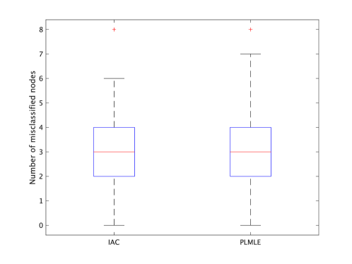
Figure 1: Number of misclassified nodes for the balanced symmetric case (Model 1). IAC and PLMLE indicate Algorithm 1 and Algorithm 3 in Gao et al. [2017], respectively. The figure is plotted with MATLAB boxplot function with outliers (the red crosses) for $100$ experiment instances.

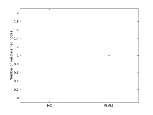
Figure 2: Number of misclassified nodes for the imbalanced case (Model 2). IAC and PLMLE indicate Algorithm 1 and Algorithm 3 in Gao et al. [2017], respectively. The figure is plotted with MATLAB boxplot function with outliers (the red crosses) for $100$ experiment instances.

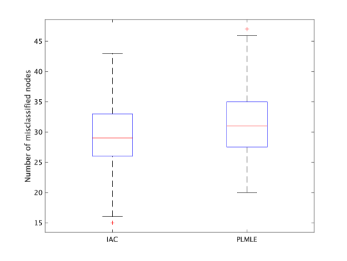
Figure 3: Number of misclassified nodes for the sparse symmetric case (Model 3). IAC and PLMLE indicate Algorithm 1 and Algorithm 3 in Gao et al. [2017], respectively. The figure is plotted with MATLAB boxplot function with outliers (the red crosses) for $100$ experiment instances.

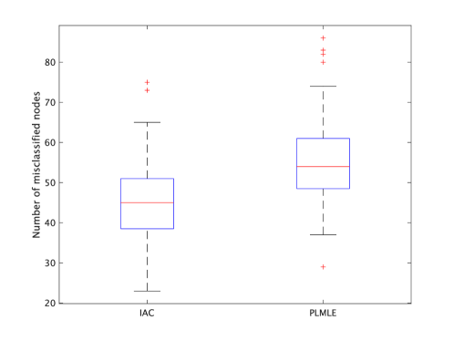
Figure 4: Number of misclassified nodes for the sparse asymmetric case (Model 4). IAC and PLMLE indicate Algorithm 1 and Algorithm 3 in Gao et al. [2017], respectively. The figure is plotted with MATLAB boxplot function with outliers (the red crosses) for $100$ experiment instances.

References

- Abbe [2018] Emmanuel Abbe. Community detection and stochastic block models. Foundations and Trends in Communications and Information Theory, 14(1–2):1–162, 2018.
- Abbe and Sandon [2015a] Emmanuel Abbe and Colin Sandon. Community detection in general stochastic block models: fundamental limits and efficient recovery algorithms. In FOCS, 2015a.
- Abbe and Sandon [2015b] Emmanuel Abbe and Colin Sandon. Recovering communities in the general stochastic block model without knowing the parameters. In NeurIPS, 2015b.
- Abbe et al. [2016] Emmanuel Abbe, Afonso S. Bandeira, and Georgina Hall. Exact recovery in the stochastic block model. IEEE Transactions on Information Theory, 62(1):471–487, 2016.
- Bordenave et al. [2015] Charles Bordenave, Marc Lelarge, and Laurent Massoulié. Non-backtracking spectrum of random graphs: Community detection and non-regular ramanujan graphs. In FOCS, 2015.
- Chatterjee [2015] Sourav Chatterjee. Matrix estimation by universal singular value thresholding. The Annals of Statistics, 43(1):177–214, 2015.
- Coja-Oghlan [2010] Amin Coja-Oghlan. Graph partitioning via adaptive spectral techniques. Combinatorics, Probability and Computing, 19(2):227–284, 2010.
- Decelle et al. [2011] Aurelien Decelle, Florent Krzakala, Cristopher Moore, and Lenka Zdeborová. Inference and phase transitions in the detection of modules in sparse networks. Physical Review Letters, 107, 2011.
- Feige and Ofek [2005] Uriel Feige and Eran Ofek. Spectral techniques applied to sparse random graphs. Random Structures & Algorithms, 27(2):251–275, 2005.
- Gao et al. [2017] Chao Gao, Zongming Ma, Anderson Y Zhang, and Harrison H Zhou. Achieving optimal misclassification proportion in stochastic block models. Journal of Machine Learning Research, 18(1):1980–2024, 2017.
- Hajek et al. [2016] Bruce Hajek, Yihong Wu, and Jiaming Xu. Achieving exact cluster recovery threshold via semidefinite programming. IEEE Transactions on Information Theory, 62(5):2788–2797, 2016.
- Halko et al. [2011] Nathan Halko, Per-Gunnar Martinsson, and Joel A. Tropp. Finding structure with randomness: Probabilistic algorithms for constructing approximate matrix decompositions. SIAM review, 53(2):217–288, 2011.
- Heimlicher et al. [2012] Simon Heimlicher, Marc Lelarge, and Laurent Massoulié. Community detection in the labelled stochastic block model. arXiv preprint arXiv:1209.2910, 2012.
- Holland et al. [1983] Paul W. Holland, Kathryn Blackmond Laskey, and Samuel Leinhardt. Stochastic blockmodels: First steps. Social Networks, 5(2):109–137, 1983.
- Kaufmann et al. [2016] Emilie Kaufmann, Olivier Cappé, and Aurélien Garivier. On the complexity of best arm identification in multi-armed bandit models. Journal of Machine Learning Research, 17:1–42, 2016.
- Krzakala et al. [2013] Florent Krzakala, Cristopher Moore, Elchanan Mossel, Joe Neeman, Allan Sly, Lenka Zdeborová, and Pan Zhang. Spectral redemption in clustering sparse networks. Proceedings of the National Academy of Sciences, 110(52):20935–20940, 2013.
- Lai and Robbins [1985] Tze Leung Lai and Herbert Robbins. Asymptotically efficient adaptive allocation rules. Advances in applied mathematics, 6(1):4–22, 1985.
- Le et al. [2017] Can M. Le, Elizaveta Levina, and Roman Vershynin. Concentration and regularization of random graphs. Random Structures & Algorithms, 51(3):538–561, 2017.
- Lelarge et al. [2013] Marc Lelarge, Laurent Massoulié, and Jiaming Xu. Reconstruction in the labeled stochastic block model. In 2013 IEEE Information Theory Workshop, 2013.
- Lindvall [2002] Torgny Lindvall. Lectures on the Coupling Method. Dover Books on Mathematics Series. Courier Corporation, 2002.
- Massoulié [2013] Laurent Massoulié. Community detection thresholds and the weak ramanujan property. In STOC, 2013.
- Mossel et al. [2015a] Elchanan Mossel, Joe Neeman, and Allan Sly. Reconstruction and estimation in the planted partition model. Probability Theory and Related Fields, 162(3):431–461, 2015a.
- Mossel et al. [2015b] Elchanan Mossel, Joe Neeman, and Allan Sly. Consistency thresholds for the planted bisection model. In STOC, 2015b.
- Newman and Girvan [2004] M. E. J. Newman and M. Girvan. Finding and evaluating community structure in networks. Physical Review E, 69:026113, 2004.
- Tao [2012] Terence Tao. Topics in random matrix theory, volume 132. American Mathematical Society, 2012.
- Tsybakov [2008] Alexandre B. Tsybakov. Introduction to Nonparametric Estimation. Springer Series in Statistics. Springer New York, NY, 2008.
- Vershynin [2018] Roman Vershynin. High-dimensional probability: An introduction with applications in data science, volume 47. Cambridge University Press, 2018.
- Wang et al. [2021] Peng Wang, Huikang Liu, Zirui Zhou, and Anthony Man-Cho So. Optimal non-convex exact recovery in stochastic block model via projected power method. In ICML, 2021.
- Yun and Proutiere [2014a] Se-Young Yun and Alexandre Proutiere. Accurate community detection in the stochastic block model via spectral algorithms. arXiv preprint arXiv:1412.7335, 2014a.
- Yun and Proutiere [2014b] Se-Young Yun and Alexandre Proutiere. Community detection via random and adaptive sampling. In COLT, 2014b.
- Yun and Proutiere [2016] Se-Young Yun and Alexandre Proutiere. Optimal cluster recovery in the labeled stochastic block model. In NeurIPS, 2016.
- Zhang and Zhou [2016] Anderson Y. Zhang and Harrison H. Zhou. Minimax rates of community detection in stochastic block models. The Annals of Statistics, 44(5):2252 – 2280, 2016.