Robust Semantic Segmentation: Strong Adversarial Attacks and Fast Training of Robust Models

Abstract

While a large amount of work has focused on designing adversarial attacks against image classifiers, only a few methods exist to attack semantic segmentation models. We show that attacking segmentation models presents task-specific challenges, for which we propose novel solutions. Our final evaluation protocol outperforms existing methods, and shows that those can overestimate the robustness of the models. Additionally, so far adversarial training, the most successful way for obtaining robust image classifiers, could not be successfully applied to semantic segmentation. We argue that this is because the task to be learned is more challenging, and requires significantly higher computational effort than for image classification. As a remedy, we show that by taking advantage of recent advances in robust ImageNet classifiers, one can train adversarially robust segmentation models at limited computational cost by fine-tuning robust backbones.

1 Introduction

The vulnerability of systems based on neural networks to adversarial perturbations, that is small changes in the input can drastically modify the output of the models, is now well-known (Biggio et al., 2013; Szegedy et al., 2014; Grosse et al., 2016; Jin et al., 2019). Among computer vision tasks, image classification is by far the one for which this phenomenon has been most extensively studied. A large amount of work has been dedicated to developing adversarial attacks in several threat models, including $\ell_{p}$-bounded perturbations (Carlini and Wagner, 2017; Chen et al., 2018; Rony et al., 2019), sparse attacks (Brown et al., 2017; Croce et al., 2022), and those defined by perceptual metrics (Wong et al., 2019; Laidlaw et al., 2021). At the same time, evaluating the adversarial robustness in semantic segmentation, arguably a very relevant vision domain, has received significantly less attention. While a few early works (Xie et al., 2017; Hendrik Metzen et al., 2017; Arnab et al., 2018) have proposed methods to generate adversarial attacks in different threat models, Gu et al. (2022); Agnihotri and Keuper (2023) have recently shown that even for the most popular $\ell_{\infty}$-bounded attacks significant improvements are possible. In particular, they suggest that the PGD attack (Madry et al., 2018), which is commonly used against image classifiers, with the sum of pixelwise cross-entropy losses as objective function might not be suitable for the case of semantic segmentation: in fact, the key difference to image classification is that for semantic segmentation we have to flip the predictions of all pixels instead of just the prediction for the image.

In this work, we make significant progress towards a better adversarial robustness evaluation in semantic segmentation: first, we propose novel loss functions and optimization schemes for this domain which are better suited to the task of flipping all pixelwise predictions; second, observing that these losses have complementary properties and thus are successful on different images, we assemble them for a more reliable robustness evaluation, similar to AutoAttack (Croce and Hein, 2020) for image classification, into the ensemble SEA and use the worst-case across attacks. With our SEA we show that clean and robust semantic segmentation models can be more than $10\%$ less robust in average pixel accuracy and up to 6% lower in mIoU than suggested by existing attacks (Gu et al., 2022; Agnihotri and Keuper, 2023).

At the same time we are interested in advancing the state-of-the-art in robust semantic segmentation. For image classification the most successful methods (Rebuffi et al., 2021; Wang et al., 2023) are based on adversarial training (Madry et al., 2018). However, for semantic segmentation Gu et al. (2022) could find only limited improvement in robustness using adversarial training compared to standard models. We show that obtaining robust segmentation models with adversarial training is indeed possible but requires larger computational effort: in fact, more epochs and attacks steps are needed. However, we show that the training effort can be significantly reduced by leveraging recent advances in training robust models on ImageNet (Debenedetti, 2022; Singh et al., 2023; Liu et al., 2023). By initializing the backbone of our segmentation model with a robust ConvNeXt, adversarially pre-trained on ImageNet, we achieve similar or better adversarial robustness at up to 6 times lower computational cost than models trained with clean initialization.

Contributions. As a summary (see also an illustration in Fig. 1), in this work

• we propose novel loss functions to generate adversarial attacks against semantic segmentation, show how to adapt the optimization algorithms to significantly improve their efficiency, and validate the findings in extensive experiments,

• we propose Segmentation Ensemble Attack (SEA), an ensemble of attacks based on complementary losses for the $\ell_{\infty}$ threat model, which improves significantly over each individual attack,

• we show how to leverage existing robust image classifiers to achieve adversarially robust segmentation models at reduced training time. To our knowledge, this provides the SOTA robust models on Pascal-Voc (Everingham et al., 2010) and the first ones on Ade20K (Zhou et al., 2019).

	clean model			our robust model
ground truth	original	target cl.: grass	target cl.: sky	original	target cl.: grass	target cl.: sky

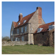
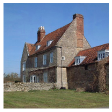
Figure 1: Effect of adversarial attacks on semantic segmentation models. For an image from the Ade20K validation set (first column, original image and ground truth mask), we show the image perturbed by targeted $\ell_{\infty}$-attacks with size $\epsilon_{\infty}=2/255$ and target classes “grass” and “sky”, and the resulting predicted segmentation maps. For a standard (clean) model, the attack is highly successful, whereas for our adversarially trained robust model the attack leads only minimal changes of the the segmentation. We use targeted attacks for illustration but untargeted attacks in the rest of the paper.

2 Related Work

Adversarial attacks for semantic segmentation. $\ell_{\infty}$-bounded attacks on segmentation models have been first proposed by Hendrik Metzen et al. (2017), which focus on targeted (universal) attacks, and Arnab et al. (2018), using FGSM (Goodfellow et al., 2015) or PGD on the cross-entropy loss. Recently, Gu et al. (2022); Agnihotri and Keuper (2023) revisited the objective function used by PGD to improve the effectiveness of $\ell_{\infty}$-bounded attacks, and are closest in spirit to our work. Additionally, there exist a few works presenting algorithms for other threat models, including unconstrained, universal and patch attacks (Xie et al., 2017; Cisse et al., 2017; Mopuri et al., 2018; Shen et al., 2019; Kang et al., 2020; Nesti et al., 2022).

Robust segmentation models. As mentioned above, limited attention has been paid to developing defenses for segmentation models. First, Xiao et al. (2018a) propose a method to detect attacks, while stating adversarial training is hard to adapt for semantic segmentation. Later, DDC-AT (Xu et al., 2021) attempts to integrate adversarial points during training exploiting additional branches to the networks, but such models are shown to be not robust by Gu et al. (2022), who also propose to use their version of PGD, named SegPGD, for adversarial training. Finally, Cho et al. (2020); Kapoor et al. (2021) present defenses based on denoising, with either Autoencoders or Wiener filters, the input to remove the adversarial perturbations before feeding it to clean models. However these methods do not provide standalone robust models. Moreover, they are tested only via attacks with limited budget, while similar techniques for protecting image classifiers have been shown ineffective once evaluated with adaptive attacks (Athalye et al., 2018; Tramèr et al., 2020).

3 Adversarial Robustness of Semantic Segmentation Models

In the following we discuss important details about the experimental setup, including the goals and constraints of the attacks, and how to measure the success of the attacks and the robustness of segmentation models. Note that some of these aspects are specific to semantic segmentation tasks, and differ from the common scenario of image classifiers.

Setup. The goal of semantic segmentation consists in classifying each pixel of a given image into the available classes (corresponding to different objects or background). We denote a segmentation model $f:\mathbb{R}^{w\times h\times c}\longrightarrow\mathbb{R}^{w\times h\times K}$, which for an image ${\bm{x}}$ of size $w\times h$ (and $c$ color channels) returns ${\bm{z}}=f({\bm{x}})$, where ${\bm{z}}_{ij}\in\mathbb{R}^{K}$ contains the score of each of the $K$ classes for the pixel ${\bm{x}}_{ij}$. Then, similar to image classification, the class predicted by $f$ for ${\bm{x}}_{ij}$ is given by ${\bm{m}}_{ij}=\mathop{\rm arg\,max}\limits_{k=1,\ldots,K}{\bm{z}}_{ijk}$, and ${\bm{m}}\in\mathbb{R}^{w\times h}$ is the segmentation map of ${\bm{x}}$. Assuming access to the ground truth map ${\bm{y}}\in\mathbb{R}^{w\times h}$, one can compute the average pixel accuracy of $f$ for ${\bm{x}}$ as $\frac{1}{w\cdot h}\sum_{i,j}\mathbb{I}({\bm{m}}_{ij}={\bm{y}}_{ij})$. Then, the goal of an adversarial attack on $f$ is to reduce its segmentation performance. This can be formalized as solving

$$\mathop{\rm min}\limits_{\bm{\delta}}\,\frac{1}{w\cdot h}\sum_{i,j}\mathbb{I}(\mathop{\rm arg\,max}\limits_{k}f({\bm{x}}+{\bm{\delta}})_{ijk}={\bm{y}}_{ij})\quad\textrm{s. th.}\quad\left\|{\bm{\delta}}\right\|_{p}\leq\epsilon,\quad{\bm{x}}+{\bm{\delta}}\in[0,1]^{w\times h\times c},$$ (1)

where one wants to minimize the number of correctly classified pixels with perturbations of bounded $\ell_{p}$-norm and remaining in the image domain. Since the objective function in Eq. (1) is non-differentiable, it is common to rephrase the problem as

$$\mathop{\rm max}\limits_{\bm{\delta}}\,\frac{1}{w\cdot h}\sum_{i,j}\mathcal{L}(f({\bm{x}}+{\bm{\delta}})_{ij},{\bm{y}}_{ij})\quad\textrm{s. th.}\quad\left\|{\bm{\delta}}\right\|_{p}\leq\epsilon,\quad{\bm{x}}+{\bm{\delta}}\in[0,1]^{w\times h\times c},$$ (2)

where $\mathcal{L}:\mathbb{R}^{K}\times\mathbb{R}\longrightarrow\mathbb{R}$ is a (almost everywhere) smooth function whose maximization induces misclassification: this can then be (approximately) solved by standard techniques for constrained optimization such as projected gradient descent (PGD). Designing surrogate losses specific for segmentation models is one of the key challenges to obtain effective attacks.

Threat model. In this work we focus on the $\ell_{\infty}$-threat model, which means that every pixel of an input image can be modified independently. It is common practice for semantic segmentation tasks to exclude the pixels belonging to the background class, which means that those are not accounted for when minimizing the training loss or computing the test performance of a model. However, it is unrealistic that an attacker only modifies non-background pixels and thus we want models which are robust for all pixels independently of how they are classified or what their ground-truth label is. Thus, we train all our models with an additional background class. Note that this does not significantly influence the clean segmentation performance, but allows us to use a more realistic definition of adversarial robustness for semantic segmentation, see App. C.3.

Metrics. For image classification the 0-1 loss is the established metric for measuring the performance of a model. Then an attacker has the clear goal of maximizing it, equivalent to reducing the classification accuracy of the model, and many techniques have been developed for this purpose (Carlini and Wagner, 2017; Madry et al., 2018). In the case of semantic segmentation, while it is possible to measure the classification accuracy averaged over pixels (Acc), it is common to use other performance metrics like Intersection over Union (IoU), averaged over classes (mIoU). Differentiable losses which approximate mIoU exist, e.g. the Dice loss (Sudre et al., 2017): however, mIoU is typically computed across all the images of the test set. This means that an attacker should optimize the perturbations over the entire set, which is not practically possible (mini-batches are often used). Conversely, the classification of pixels of an image is independent of other images, and so are the perturbations. Moreover, if an attacker is able to get all pixels to be misclassified, then the mIoU is trivially 0%. For this reason we use average accuracy as main metric for developing our attacks, but we always report mIoU as well. When reporting the worst-case over multiple runs, we select for each image the perturbation which yields the lowest average accuracy, and use it to compute the mIoU.

4 Adversarial Attacks on Segmentation Models

Before developing methods to obtain adversarially robust models, it is necessary to have effective attacks to test their robustness. Projected gradient descent (PGD) (Madry et al., 2018), together with its variants, is the most popular choice to solve the optimization problem in Eq. (2) and generate adversarial perturbations with bounded $\ell_{p}$-norm. In fact, PGD is also the basis of the existing attacks for semantic segmentation of Gu et al. (2022); Agnihotri and Keuper (2023), who argue that the cross-entropy loss is not suitable for effective attacks and thus propose novel loss functions. While we explore also the effect of different losses to create effective complementary attacks, we first show that with minimal adjustments it is possible to modify Auto-PGD (APGD) (Croce and Hein, 2020), introduced in the context of image classification, for attacks on semantic segmentation, yielding consistent improvements over PGD. Finally, we introduce our novel ensemble-attack SEA for a reliable evaluation of adversarial robustness of semantic segmentation.

4.1 Loss functions

While the only goal of adversarial attacks on image classifiers is to change the decision for a given target image, in the case of semantic segmentation an attacker wants to get as many pixels as possible to be misclassified. This is exemplified by the objective function in Eq. (1) consisting in the sum of pixelwise losses. However, this sum of losses can give rise to conflicting descent directions for different pixels, which can hinder the overall optimization. Moreover, the attack should not try to further reduce the loss for a misclassified pixel, but rather focus on the pixels with correct prediction.

In the following we give a short overview of the loss functions which have been used in the literature and the ones which we propose as new alternatives. We denote ${\bm{u}}\in\mathbb{R}^{K}$ the logits of each pixel, and $y\in\mathbb{N}$ its correct label. Moreover, given ${\bm{u}}$, we indicate as ${\bm{p}}\in\mathbb{R}^{K}$ the predicted probability distribution via the softmax function: ${\bm{p}}_{r}=e^{{\bm{u}}_{r}}/\sum_{l=1}^{K}e^{{\bm{u}}_{l}}$, $r=1,\ldots,K.$

Losses used in previous work for attacks on semantic segmentation

Cross-entropy (CE):

the most common choice as objective function in PGD based attacks is the cross-entropy between the one-hot encoding of the ground truth label and the softmax of the logits, i.e. $\mathcal{L}_{\textrm{CE}}({\bm{u}},y)=-\log{\bm{p}}_{y}=-{\bm{u}}_{y}+\log\left(\sum_{j=1}^{K}e^{{\bm{u}}_{j}}\right)$. Maximizing this loss means that one minimizes the confidence of the correct class. The cross-entropy loss is unbounded, which is problematic for semantic segmentation as already misclassified pixels will still be optimized instead of focusing on still correctly classified pixels (see discussion for the Jensen-Shannon-divergence).

Balanced cross-entropy:

Gu et al. (2022) propose to balance the importance of the cross-entropy loss of correctly and wrongly classified pixels over iterations. In particular, at iteration $t=1,\ldots,T$, they use, with $\lambda(t)=(t-1)/(2T)$,

$$\mathcal{L}_{\textrm{Bal-CE}}({\bm{u}},y)=\left((1-\lambda(t))\cdot\mathbb{I}(\mathop{\rm arg\,max}\limits_{j=1,\ldots,K}{\bm{u}}_{j}=y)+\lambda(t)\cdot\mathbb{I}(\mathop{\rm arg\,max}\limits_{j=1,\ldots,K}{\bm{u}}_{j}\neq y)\right)\cdot\mathcal{L}_{\textrm{CE}}({\bm{u}},y).$$

In this way the algorithm first focuses only on the correctly classified pixels and then progressively balances the attention given to the two subset of pixels: this has the goal of avoiding to make updates which find new misclassified pixels but leads to correct decisions for already misclassified pixels.

Weighted cross-entropy:

Agnihotri and Keuper (2023) propose to weigh the importance of the pixels via cosine similarity between the prediction vector (after applying the sigmoid function $\sigma(t)=1/(1+e^{-t})$) and the one-hot encoding ${\bm{e}}_{y}$ of the ground truth class. This can be written as

$$\mathcal{L}_{\textrm{CosSim-CE}}({\bm{u}},y)=\frac{\left\langle\sigma({\bm{u}}),{\bm{e}}_{y}\right\rangle}{\left\|\sigma({\bm{u}})\right\|_{2}\left\|{\bm{e}}_{y}\right\|_{2}}\cdot\mathcal{L}_{\textrm{CE}}({\bm{u}},y)=\sigma({\bm{u}}_{y})/\left\|\sigma({\bm{u}})\right\|_{2}\cdot\mathcal{L}_{\textrm{CE}}({\bm{u}},y),$$

and again has the effect of reducing the importance of the pixels which are confidently misclassified.

Novel losses for attacks on semantic segmentation

Masked cross-entropy:

in order to avoid over-optimizing misclassified pixels one can apply a mask which excludes such pixels from the loss computation, that is

$$\mathcal{L}_{\textrm{Mask-CE}}=\mathbb{I}(\mathop{\rm arg\,max}\limits_{j=1,\ldots,K}{\bm{u}}_{j}=y)\cdot\mathcal{L}_{\textrm{CE}}({\bm{u}},y).$$

The downside of using such a mask is that the loss becomes discontinuous and ignoring misclassified pixels might lead to changes which revert back wrongly classified pixels into correctly classified ones with the danger of creating a situation where one starts oscillating. We note that Hendrik Metzen et al. (2017) proposed, for targeted attacks, to not optimize the loss for pixels already classified into the target class with confidence higher than a fixed threshold. Similarly Xie et al. (2017) did not include the pixels already belonging to the target class in the loss computation for unconstrained attacks. However, the masked CE-loss has not been thoroughly explored for $\ell_{\infty}$-bounded untargeted attacks.

Jensen-Shannon (JS) divergence:

an intermediate behavior between losses which do not consider whether the attack is successful on a certain pixel and the classification mask used above would adjust the importance in the updates of each pixel depending on the confidence in the correct class. Given two distributions ${\bm{p}}$ and ${\bm{q}}$, the Jensen-Shannon divergence is defined as

$$D_{\textrm{JS}}({\bm{p}}\,\|\,{\bm{q}})=\left(D_{\textrm{KL}}({\bm{p}}\,\|\,{\bm{m}})+D_{\textrm{KL}}({\bm{q}}\,\|\,{\bm{m}})\right)/2,\quad\textrm{with}\quad{\bm{m}}=({\bm{p}}+{\bm{q}})/2,$$

where $D_{\textrm{KL}}$ indicates the Kullback–Leibler divergence. If we assume ${\bm{p}}$ to be the softmax output of the logits ${\bm{u}}$ and ${\bm{q}}$ the one-hot encoding of the target $y$, we get $\mathcal{L}_{\textrm{JS}}({\bm{u}},y)=D_{\textrm{JS}}({\bm{p}}\,\|\,{\bm{q}})$. Since $D_{\textrm{JS}}$ measures the similarity between the two distributions ${\bm{p}}$ and ${\bm{q}}$, maximizing $\mathcal{L}_{\textrm{JS}}$ drives the prediction of the model away from the ground truth. Unlike the KL divergence or the CE loss, the JS divergence is bounded, which means that the influence of every pixel is limited. In particular, it has the following property (see App. A for a proof)

$$\lim_{{\bm{p}}_{y}\rightarrow 0}\frac{\partial\mathcal{L}_{\textrm{JS}}({\bm{u}},y)}{\partial{\bm{u}}_{t}}=0,\quad\textrm{for}\quad t=1,\ldots,K$$

In contrast, the CE loss has a non-zero gradient if ${\bm{p}}_{y}\rightarrow 0$: thus, even clearly misclassified pixels still influence the optimization of the loss, hence one has to use masking. For the JS-divergence this is not necessary as misclassified pixels with ${\bm{p}}_{y}$ being small do not significantly influence the gradient, and thus the attack can focus on pixels which are not successfully perturbed yet without any mask.

Masked spherical loss:

using the softmax output of a classifier can make, in some circumstances, the attack (partially) fail or weaker (Croce and Hein, 2020). A more direct approach is to minimize the logit of the correct class. However, we found it to work better when projecting the logits on the unit sphere: this recovers the structure of the spherical scoring rule (Bickel, 2007) which is a proper multi-class loss. We hypothesize that the projection first brings the logits of different pixels on the same scale, which balances the gradients deriving from each of them, and, second, involves the logits of all classes in the loss as part of the denominator. Since this loss is directly targeted to misclassification, we use it in combination with the mask for misclassified pixels:

$$\mathcal{L}_{\textrm{Mask-Sph.}}=-\mathbb{I}(\mathop{\rm arg\,max}\limits_{j=1,\ldots,K}{\bm{u}}_{j}=y)\cdot{\bm{u}}_{y}/\left\|{\bm{u}}\right\|_{2}.$$

Table 1: APGD consistently outperforms PGD for two existing attacks, SegPGD (Gu et al., 2022) and CosPGD (Agnihotri and Keuper, 2023), on semantic segmentation. We report average pixel accuracy and mIoU after the adversarial attack, at various strengths of $\epsilon_{\infty}$.

$\epsilon_{\infty}$	$\mathcal{L}_{\textrm{Bal-CE}}$				$\mathcal{L}_{\textrm{CosSim-CE}}$
	SegPGD		SegAPGD		CosPGD		CosAPGD
	Acc	mIoU	Acc	mIoU	Acc	mIoU	Acc	mIoU
4/255	88.6	65.0	88.7	64.8	89.0	65.5	88.9	65.4
8/255	74.6	39.4	74.2	41.3	78.2	47.5	77.8	47.3
12/255	45.8	15.0	43.3	14.9	58.2	28.3	56.2	26.4
16/255	26.2	7.1	20.7	5.7	38.0	17.2	34.0	15.3

4.2 APGD for semantic segmentation attacks

Projected gradient descent (PGD) (Madry et al., 2018) uses the following iterative scheme for minimizing an objective function $g$ in the set $S=\{z\in\mathbb{R}^{d}:\left\|z-x\right\|_{\infty}\leq\epsilon,\,z\in[0,1]^{d}\}$, i.e. an $\ell_{\infty}$-ball around a given point $x$ intersected with the image box, denoting by $P_{S}$ the projection onto $S$:

$$x^{(t+1)}=P_{S}\left(x^{(t)}-\alpha^{(t)}\mathop{\rm sign}\limits(\nabla g(x^{(t)}))\right).$$

APGD has been introduced in Croce and Hein (2020) as an improved version of standard PGD which does not require parameter tuning e.g. selection of the step size $\alpha^{(t)}$. While it has been used in attacks for image classification, it can be more generally applied as optimizer for constrained problems. We show in Table 1 that simply replacing PGD with APGD for two previously proposed losses consistently improves their performance on a robust model from Sec. 5 (both PGD and APGD use 100 iterations, see App. B for details). The two attacks we consider are: i) SegPGD (Gu et al., 2022), an attack which optimizes $\mathcal{L}_{\textrm{Bal-CE}}$ with PGD, and ii) CosPGD (Agnihotri and Keuper, 2023), an attack which optimizes $\mathcal{L}_{\textrm{CosSim-CE}}$ with PGD. We observe that for both attacks and all values of the radius $\epsilon$, APGD yields lower average pixel accuracy and mIoU (in grey), without imposing extra costs during optimization. Note that for high values of $\epsilon$ the improvements are quite large. Thus we use APGD for the optimization of all losses in this paper.

4.3 Complementary performance of different losses for varying attack radii

Table 2: Comparison of losses at different robustness levels. We use each of the losses discussed in Sec. 4.1 as objective in APGD with 100 iterations on one clean and one robust model. We report average pixel accuracy and mIoU (clean performance is indicated next to the model name). Depending on the radius $\epsilon_{\infty}$, the best results are realized by different losses. The worst-case over all runs is often significantly lower than each individual one.

$\epsilon_{\infty}$	losses used in prior works						proposed losses						Worst case
	$\mathcal{L}_{\textrm{CE}}$		$\mathcal{L}_{\textrm{Bal-CE}}$		$\mathcal{L}_{\textrm{CosSim-CE}}$		$\mathcal{L}_{\textrm{JS}}$		$\mathcal{L}_{\textrm{Mask-CE}}$		$\mathcal{L}_{\textrm{Mask-Sph.}}$		over losses
Clean model  (93.4  77.2)
0.25/255	77.3	48.3	74.0	43.7	76.6	48.0	73.9	44.3	73.2	42.7	75.8	44.4	71.1	39.9
0.5/255	49.3	25.1	42.3	18.5	46.9	24.0	39.4	18.3	36.9	14.9	37.5	14.5	32.5	12.1
1/255	21.2	9.9	13.9	4.8	17.2	8.1	9.1	4.0	7.9	2.2	6.6	1.6	5.3	1.2
2/255	7.4	4.0	2.9	1.5	3.4	2.3	0.5	0.4	0.3	0.2	0.1	0.1	0.1	0.0
Adversarially trained classifier  (92.7  75.9)
4/255	88.9	65.7	88.7	64.8	88.9	65.4	88.4	64.8	88.9	65.6	90.4	69.7	88.3	64.4
8/255	78.9	48.9	74.2	41.3	77.8	47.3	75.3	43.5	74.6	41.8	80.3	49.6	72.3	38.4
12/255	59.9	28.9	43.3	14.9	56.6	26.4	45.1	18.6	38.8	13.2	38.9	12.1	31.9	8.4
16/255	41.5	18.1	20.7	5.7	34.0	15.3	19.1	7.4	12.9	3.4	8.4	2.0	6.4	1.1

In Table 2 we compare the effectiveness of the attacks (all using APGD) based on existing or proposed losses for a standard and an adversarially trained semantic segmentation model on Pascal-Voc (details in Sec. 5). We are mainly interested in the attack performance across different radii $\epsilon$ for the $\ell_{\infty}$-threat model. We note that the best attack/loss depends on the radius, and is almost always achieved by one of our novel proposed losses. In particular, existing attacks have problems when using large $\epsilon$ values, as already observed in Agnihotri and Keuper (2023). When considering the image-wise worst attack regarding accuracy, we see that there is quite a gap between the worst-case over all attacks and the best single attack. This motivates our ensemble of attacks discussed next.

4.4 Segmentation Ensemble Attack (SEA)

Progressive radius reduction. In Table 2 we see that the worst case over losses is significantly lower than each individual attack. Besides the complementarity of the losses, this suggests that the optimization algorithm faces some issue regardless of the objective function, and can get stuck in suboptimal local minima. At the same time, increasing the perturbation set, i.e. larger $\epsilon_{\infty}$, reduces robust accuracy, which means that the gradient information provided by the models are still valid (no gradient masking is occurring). Thus, we take inspiration from Croce and Hein (2021), who adapted APGD to the $\ell_{1}$-threat model. In that case, the complex geometry of the $\ell_{1}$-ball intersected with the image box $[0,1]^{d}$ leads to difficulties in the optimization, which are mitigated by running the attack with larger radii and using the results, projected on the feasible set, as starting points for the algorithm with the final target radius $\epsilon_{1}$. In the case of semantic segmentation, we hypothesize that jointly optimizing the loss of thousands of pixels raises similar issues, and thus we adapt this technique to our task: we split the budget of iterations into three slots (with ratio $3:3:4$) where we run the attack with $2\cdot\epsilon_{\infty}$, $1.5\cdot\epsilon_{\infty}$ and $\epsilon_{\infty}$ respectively. The best adversarial attack found during each stage is then projected onto the smaller $\ell_{\infty}$-ball to start the algorithm in the next stage.

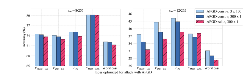
Figure 2: Testing difference between const-$\epsilon$ and red-$\epsilon$ schemes. Under the same iteration budget for the robust init. AT⁵ model, across different losses we see radius reduction (red-$\epsilon$) scheme leads to most drop in robust Acc. Specifically for worst-case over all losses, red-$\epsilon$ leads to the best attack across different perturbation strengths. The same trend holds for mIoU, see Fig. 3 in App. C.1

Radius reduction vs more iterations. To assess the effectiveness of the scheme with progressive reduction of the radius $\epsilon$ (red-$\epsilon$) described above, we compare it with 300 iterations to the original APGD scheme (const-$\epsilon$) of either 300 iterations or 100 iterations and 3 random restarts, so that all schemes have the same computational budget. We show in Fig. 2 the robust accuracy achieved by the three attacks with different objective functions, for $\epsilon_{\infty}\in\{8/255,12/255\}$, on the adversarially trained model on Pascal-Voc. One can observe that the red-$\epsilon$ APGD yields the best results (lowest accuracy) for almost every case, with large improvements especially at $\epsilon_{\infty}=12/255$. This suggests that this scheme is better suited for generating stronger attacks on semantic segmentation models than common options used in image classification like more iterations or random restarts.

Final scheme. Distilling the findings of the complementary nature of the various losses at different robustness levels and the improvement in the optimization algorithm provided by the scheme with progressive radius shrinkage, we propose Segmentation Ensemble Attack, or SEA, as an evaluation protocol for segmentation models. It includes four runs of 300 iterations with red-$\epsilon$ APGD optimizing each of the four best losses found above, namely $\mathcal{L}_{\textrm{Mask-CE}}$, $\mathcal{L}_{\textrm{Bal-CE}}$, $\mathcal{L}_{\textrm{JS}}$ and $\mathcal{L}_{\textrm{Mask-Sph}}$. The motivation for this choice comes from the fact that the worst-case over these four losses leads to maximum $0.1\%$ higher robust average accuracy or mIoU than using all six losses, and thus the two left-out losses, $\mathcal{L}_{\textrm{CE}}$ and $\mathcal{L}_{\textrm{CosSim-CE}}$, do not add further value (see App. C.1). We analyze in details the importance of each component of SEA with a breakdown of the performance in App. C.1.

5 Adversarially Robust Segmentation Models

Adversarial training (AT) (Madry et al., 2018) aims at making models robust by adversarially perturbing the training points and minimizing the training loss on them. In the following we discuss methods for robust segmentation models presented by prior work, and propose to take advantage of pre-trained robust classifiers to obtain robust segmentation models. We do standard adversarial training using PGD on the cross-entropy loss with an $\ell_{\infty}$-threat model of radius $\epsilon_{\infty}=4/255$ (as used by robust classifiers on ImageNet). All evaluations are carried out with our SEA on the entire validation set. Training and evaluation details can be found in App. B.

5.1 Existing work on adversarially robust semantic segmentation models

As mentioned above, unlike for image classification, only a few works have applied adversarial training to obtain robust segmentation models. Gu et al. (2022) do adversarial training with 3 or 7 steps of their SegPGD at $\epsilon_{\infty}=8/255$, using a ResNet-50 as backbone in a PSPNet (Zhao et al., 2017) architecture. However, the obtained adversarial robustness, see upper part of Table 3, is relatively low. Since the models are not available, we can only show the robustness values reported in their paper which are based on the original SegPGD attack and not evaluated using SEA, but one can see that the improvement in mIoU provided by AT⁷ is smaller than 14% compared to the clean model. Moreover, under the evaluation with SEA our clean model has no robustness already at $\epsilon=4/255$ (and likely at smaller ones as one can infer from Table 1), suggesting that the reported robustness for the models from Gu et al. (2022) might be overestimated and would significantly decrease with SEA.

Table 3: Comparison of training schemes for Pascal-Voc. For each model and $\epsilon_{\infty}$ value we report robust average pixel accuracy (white background columns) and mIoU (grey background columns) given by our SEA. * indicates that the result is taken from the original paper (since the model is not available) and obtained using a weaker attack.

Training scheme			0		4/255		8/255		12/255		16/255
PSPNet with ResNet-50 backbone (previous works)
clean (Gu et al., 2022)			–	76.6	–	–	–	3.4*	–	–	–	–
AT3 (Gu et al., 2022)			–	75.4	–	–	–	10.3*	–	–	–	–
AT7 (Gu et al., 2022)			–	74.4	–	–	–	17.0*	–	–	–	–
UPerNet with ConvNeXt-T backbone (ours)
clean			93.4	77.2	0.0	0.0	0.0	0.0	0.0	0.0	0.0	0.0
AT2	clean init.	50 ep.	93.4	77.4	2.6	0.1	0.0	0.0	0.0	0.0	0.0	0.0
AT2	clean init.	300 ep.	93.1	76.3	86.5	59.6	44.1	16.6	4.6	0.1	0.0	0.0
AT2	robust init.	50 ep.	92.9	75.9	86.7	60.8	50.2	21.0	9.3	2.4	0.8	0.3
AT5	clean init.	50 ep.	91.9	73.1	86.2	59.2	64.6	28.3	20.7	4.9	2.0	0.4
AT5	clean init.	300 ep.	92.8	75.5	88.6	64.4	71.4	37.7	23.4	6.6	2.7	0.6
AT5	robust init.	50 ep.	92.7	75.2	88.3	63.8	71.2	37.0	27.4	8.1	4.2	0.9

5.2 Robust models via robust initialization

Since Liu et al. (2022) showed that their ConvNeXt, one of the currently most popular architectures for vision tasks, is very effective also for semantic segmentation, we use it as backbone in UPerNet (Xiao et al., 2018b). Moreover, Singh et al. (2023) have recently shown substantial improvements in adversarial training on ImageNet using the ConvNeXt architecture. In particular, we follow them and replace the PatchStem of the ConvNeXt with a ConvStem for improved robustness when using adversarial training without affecting performance of clean training. We use here ConvNeXt-T (similar size as ResNet-50), and present the results for the larger ConvNeXt-S backbones in App. C.2 and other architectures in App. C.4.

Pascal-Voc. Table 3 reports the statistics about the robustness of the various models trained on Pascal-Voc. First, we use a ConvNeXt given by clean pre-training on ImageNet as initialization for the backbone (the decoder is randomly initialized). When using 2 steps of PGD for generating the perturbations for training (denoted as AT²), 50 epochs of adversarial training are not sufficient to achieve non-trivial robustness. However, increasing the length of training to 300 epochs makes the model significantly more robust. This suggests that learning robust segmentation models is a challenging problem. Then, in order to give a warm start to the training algorithm, we initialize the backbone with a robust image classifiers, adversarially trained on ImageNet at $\epsilon_{\infty}=4/255$. 50 epochs of AT² from robust initialization leads to 86.7% of robust accuracy at $\epsilon_{\infty}=4/255$, and above 50% at $\epsilon_{\infty}=8/255$ (while having only 0.5% lower clean accuracy than the clean model which however shows 0% of robustness). This is significantly better than using 300 epochs from clean initialization. Moreover, it already exceeds, even compared to their original evaluation, the results reported by Gu et al. (2022). We further test the effect of increasing the number of steps for training from 2 to 5 (AT⁵), which doubles the computational cost per epoch. In this case, even 50 epochs from clean initialization give a model with good robustness, which again improves with 300 epochs. Even with AT⁵, using the robust initialization allows us to match (or outperform at large $\epsilon$ values) with 50 epochs the robustness of the models with clean initialization and 300 epochs. This shows that robust classifiers, commonly available, can significantly help in reducing the cost of getting robust segmentation models. Finally, our models show more than 2x higher robustness than reported in Gu et al. (2022). Interestingly, the large gains in robustness do not degrade much the clean performance, which is a typical drawback of adversarial training.

Table 4: Comparison of training schemes for Ade20K. We repeat the evaluation from Table 3 on Ade20K, for which no previous work presented robust models. We show robust accuracy and mIoU evaluated with SEA. All models are UPerNet with ConvNeXt-T backbone.

Training scheme			0		4/255		8/255		12/255
clean		128 ep.	75.5	41.1	0.0	0.0	0.0	0.0	0.0	0.0
AT2	clean init.	128 ep.	73.4	36.4	0.2	0.0	0.0	0.0	0.0	0.0
AT2	robust init.	128 ep.	72.0	34.7	46.0	15.4	6.0	1.8	0.0	0.0
AT5	clean init.	128 ep.	68.0	26.1	52.4	14.0	24.7	4.7	2.4	0.3
AT5	robust init.	32 ep.	68.8	25.2	55.4	15.6	28.3	5.9	3.8	0.7
AT5	robust init.	128 ep.	70.5	31.7	55.6	18.6	26.4	6.7	3.3	0.8

Ade20K. We further test the effectiveness of our scheme for obtaining robust models on the more challenging Ade20K dataset, with 150 object classes compared to 20 of Pascal-Voc (plus background class). We remark that, as discussed in Sec. 3, we train our models to predict also a background class, and similarly the attacks can use it to induce misclassification. Table 4 shows that, consistently with Pascal-Voc, 128 epochs (used following Liu et al. (2022)) of AT² from clean initialization are not sufficient to obtain a robust model, while they are when using robust initialization. For AT⁵, the model initialized with the robust backbone has higher clean and robust performance than that with standard backbone. To test whether the robust initialization allows us to save training time, we additionally report a model trained for only 32 epochs: it outperforms the one from clean initialization with 4x lower computational cost. Moreover, it has similar performance to the model with 128 epochs and robust initialization in the target threat model ($\epsilon=4/255$), while it trades-off some clean performance for robustness at higher radii (longer training can fit better the training data, improving clean accuracy). We highlight that ours are the first adversarially trained models reported for Ade20K, which explains the lack of baselines.

6 Conclusion

We have shown that adversarial attacks on semantic segmentation models can be improved by adapting the optimization algorithms and objective functions, developing SEA, an ensemble of attacks which outperforms existing methods. This may open new research directions, for example for losses which take into account the interaction of neighboring pixels or directly target mIoU to achieve stronger attacks. Moreover, we could train segmentation models with SOTA robustness, even at limited computational cost by taking advantage of adversarially pre-trained image classifiers. It will be interesting to analyze the properties of such models, as well as testing the effect of applying our method to other architectures.

Limitations. We consider SEA an important step towards strong evaluation of robustness for semantic segmentation models. However, as shown for image classification (Croce and Hein, 2020), PGD-based attacks should be complemented by white-box attacks of different type and especially black-box methods. Moreover, several techniques, e.g. using different loss functions, unlabeled and synthetic data, adversarial weight perturbations, etc., have been shown effective to achieve more robust classifiers, and might be similarly beneficial for segmentation. Testing all these options is out of scope for our work, but might improve the robustness of segmentation models.

Broader Impact

We propose new techniques to test the robustness of segmentation models to adversarial attacks. While we consider it important to estimate the vulnerability of existing systems, such methods might potentially be used by malicious actors. However, we also provide insights on how to obtain, at limited computational cost, models which are robust to such perturbations.

Appendix A Proof of the Property of the Jensen-Shannon-Divergence

The Jensen-Shannon-divergence between the predicted distribution $p$ and the label distribution $q$ is given by

$$D_{\textrm{JS}}({\bm{p}}\,\|\,{\bm{q}})=\left(D_{\textrm{KL}}({\bm{p}}\,\|\,{\bm{m}})+D_{\textrm{KL}}({\bm{q}}\,\|\,{\bm{m}})\right)/2,\quad\textrm{with}\quad{\bm{m}}=({\bm{p}}+{\bm{q}})/2,$$

Assuming that we have a one-hot label encoding ${\bm{q}}=e_{y}$ (where $e_{y}$ is the $y$-th cartesian coordinate vector), one gets

$$D_{\textrm{JS}}({\bm{p}}\,\|\,e_{y})=\frac{1}{2}\log\left(\frac{2}{1+{\bm{p}}_{y}}\right)+\frac{1}{2}\sum_{i=1}^{K}{\bm{p}}_{i}\log\left(\frac{2{\bm{p}}_{i}}{\delta_{yi}+{\bm{p}}_{i}}\right).$$

Then

$$\frac{\partial D_{\textrm{JS}}({\bm{p}}\,\|\,e_{y})}{\partial{\bm{p}}_{r}}=-\frac{1}{1+{\bm{p}}_{y}}\delta_{yr}+\log\left(\frac{2{\bm{p}}_{r}}{\delta_{yr}+{\bm{p}}_{r}}\right)+1-\frac{{\bm{p}}_{r}}{\delta_{yr}+{\bm{p}}_{r}}=\begin{cases}\log\left(\frac{2{\bm{p}}_{y}}{1+{\bm{p}}_{y}}\right)&\textrm{ if }r=y,\\ \log(2)&\textrm{ else }.\end{cases}$$

Given the logits $u$ we use the softmax function

$${\bm{p}}_{r}=\frac{e^{u_{r}}}{\sum_{t=1}^{K}e^{u_{t}}},\quad r=1,\ldots,K,$$

to obtain the predicted probability distribution ${\bm{p}}$. One can compute:

$$\frac{\partial{\bm{p}}_{r}}{\partial u_{t}}=\delta_{rt}{\bm{p}}_{t}-{\bm{p}}_{r}{\bm{p}}_{t}\quad\Longrightarrow\quad\sum_{r=1}^{K}\frac{\partial{\bm{p}}_{r}}{\partial u_{t}}=0$$

Then

$$\frac{\partial D_{\textrm{JS}}({\bm{p}}\,\|\,e_{y})}{\partial u_{t}} =\sum_{r=1}^{K}\frac{\partial D_{\textrm{JS}}({\bm{p}}\,\|\,e_{y})}{\partial{\bm{p}}_{r}}\frac{\partial{\bm{p}}_{r}}{\partial u_{t}}=\log\left(\frac{2{\bm{p}}_{y}}{1+{\bm{p}}_{y}}\right)\frac{\partial{\bm{p}}_{y}}{\partial u_{t}}+\log(2)\sum_{r\neq y}\frac{\partial{\bm{p}}_{r}}{\partial u_{t}}$$

$$=\log\left(\frac{2{\bm{p}}_{y}}{1+{\bm{p}}_{y}}\right)\frac{\partial{\bm{p}}_{y}}{\partial u_{t}}-\log(2)\frac{\partial{\bm{p}}_{y}}{\partial u_{t}}=\log\left(\frac{{\bm{p}}_{y}}{1+{\bm{p}}_{y}}\right)\left[\delta_{yt}{\bm{p}}_{y}-{\bm{p}}_{y}{\bm{p}}_{t}\right]$$

$$={\bm{p}}_{y}\log\left(\frac{{\bm{p}}_{y}}{1+{\bm{p}}_{y}}\right)\left[\delta_{yt}-{\bm{p}}_{t}\right]$$

Noting that $\lim_{x\rightarrow 0}x\log(x)=0$ we get the result that: $\lim\limits_{{\bm{p}}_{y}\rightarrow 0}\frac{\partial D_{\textrm{JS}}({\bm{p}}\,\|\,e_{y})}{\partial u_{t}}=0.$ We note that this is in contrast to the cross-entropy loss where, $\mathcal{L}_{\textrm{CE}}({\bm{p}},e_{y})=-\log{\bm{p}}_{y}$, and

$$\frac{\partial\mathcal{L}_{\textrm{CE}}({\bm{p}},e_{y})}{\partial u_{t}}=-\delta_{yt}+{\bm{p}}_{t}$$

and thus $\lim\limits_{{\bm{p}}_{y}\rightarrow 0}\frac{\partial\mathcal{L}_{\textrm{CE}}({\bm{p}},e_{y})}{\partial u_{t}}\neq 0$. In particular, this implies that when optimizing the sum of the cross-entropy loss over all pixels, even pixels which are already successfully attacked will still influence the gradient. In contrast, for the Jensen-Shannon-divergence the pixels which are already successfully attacked (${\bm{p}}_{y}$ is small) do not contribute anymore significantly to the gradient and thus the attack can focus on the pixels which are not yet successfully attacked without the need of masking.

Appendix B Experimental Details

We here provide additional details about both attacks and training scheme used in the experiments in the main part. The code and robust models are publicly available here.

B.1 Attacks for semantic segmentation

Baselines. Since Gu et al. (2022); Agnihotri and Keuper (2023) do not provide code for their methods, we re-implement both SegPGD and CosPGD following the indications in the respective papers and personal communication with the authors of CosPGD. In the comparison in Table 1, we use PGD with step size 0.01 and 100 iterations. Moreover, we select for each image the iterate with highest loss.

APGD with masked losses. Since APGD relies on the progression of the objective function value to e.g. select the step size, using losses which mask the misclassified pixels might be problematic, since the loss is not necessarily monotonic. Then, in practice we only apply the mask when computing the gradient at each iteration.

B.2 Training robust models

In the following, we detail the employed network architectures, as well as our training procedure for the utilized datasets. All experiments are conducted in multi-GPU setting with PyTorch library. For adversarial training we use PGD at $\epsilon=4/255$ and step size 0.01. When doing clean training, the backbones are initialized with clean models pre-trained on ImageNet.

Model architectures. Semantic segmentation model architectures have adapted to use image classifiers in their backbone. Given UPerNet coupled with ConvNeXt (Liu et al., 2022) and/or transformer models like Swin (Liu et al., 2021) achieves art segmentation results, we use UPerNet as the base architecture for our experiments with ConvNeXt as the backbone. For both clean and robust initialization setups, we use the ImageNet-1k pre-trained weights from Singh et al. (2023). Singh et al. (2023) achieve art robustness for $\ell_{\infty}$-threat model at $\epsilon=4/255$ on the ImageNet-1k dataset. They propose some architectural changes, notably replacing PatchStem with a ConvStem in their most robust ConvNeXt models, and we keep these changes intact in our backbone models. We highlight that ConvNeXt-T, when adversarially trained for classification on ImageNet, attains significantly higher robustness than ResNet-50 at a similar parameter and FLOPs count. For example, at $\epsilon_{\infty}=4/255$, the ConvNeXt-T we use has 49.5% of robust accuracy, while ResNet-50 is reported to achieve around 35% (Bai et al., 2021; Singh et al., 2023). This supports choosing ConvNeXt as backbone for obtaining robust segmentation models.

Training setup for Pascal-Voc. For training on the Pascal-Voc dataset, we use the augmentation setup from Hariharan et al. (2011). Our training set comprises of 8498 images and we validate on the original Pascal-Voc validation set of 1449 images. For both training and testing the image is cropped from a base size of 512x512 to 473x473, we employ random horizontal flip and Gaussian Blur as the only two augmentations on top as done by  (Zhao et al., 2017). We use the auxiliary head, with a loss coefficient of 0.4 in training the model. We train robust-initialized models only for 50 epochs whereas for clean initialized models we have other configurations as well. Adversarial training is done with either 2 or 5 steps of PGD on the cross-entropy loss. Throughout all experiments the base learning rate (LR) of 1e-3 with AdamW (Loshchilov and Hutter, 2019) optimizer and a weight decay factor of 1e-2 is used. We employ linear LR decay with a warm-up of 10 epochs for 50 epoch runs. Wherever we train for more than 50 epochs we linearly scale the warm-up epochs as well. For testing, we keep the same resolution resizing as for training without the augmentations and use the single-scale approach. Unlike most other works in literature, we train for 21 classes (including the background class).

Training setup for Ade20K. We use the full standard training and validation sets from Zhou et al. (2019). For both training and testing the image is resized to 520x520, then cropped to 512x512, keeping the same augmentations as for Pascal-Voc. We train for 128 epochs (for clean and adversarial training) with a base LR of 1e-4 with AdamW optimizer and a weight decay factor of 5e-2, as used for the original ConvNeXt backbone UPerNet by Liu et al. (2022). We employ linear LR decay with a warm-up of 20 epochs and use stochastic depth coefficient of 0.4 or 0.3 depending on the backbone, same as the original work. We do not use heavier augmentations and LayerDecay (Bao et al., 2021) optimizer as done by Liu et al. (2022). For the 32 epoch run in Table 4, we do a warm-up of 5 epochs, while the other parameters are the same as for 128 epochs. Unlike the original work we train with 151 classes (including the background class).

Appendix C Additional Experiments

We present additional studies of the properties of our SEA scheme and of the robust models.

Table 5: Loss selection for SEA. We compare taking the worst-case over all six losses from Table 2 APGD with 100 iterations versus using only the subset of the four losses part of SEA (average accuracy and mIoU are shown). The models are clean or adversarially trained for Pascal-Voc. Leaving out two losses does not substantially impact the performance while considerably reduces the computational cost.

Subset	$\epsilon_{\infty}\rightarrow$	4/255		8/255		12/255		16/255
model: clean, 50 epochs
all losses		71.1	39.9	32.5	12.1	5.3	1.2	0.1	0.0
four losses		71.2	40.0	32.6	12.1	5.3	1.2	0.1	0.0
model: AT5, robust init., 50 epochs
all losses		88.3	64.4	72.3	38.4	31.9	8.4	6.4	1.1
four losses		88.3	64.6	72.3	38.4	31.9	9.0	6.4	1.2

C.1 Analysis of SEA

Selection of losses. In Table 2 we have shown the performance of the attacks (APGD with 100 iterations) with six loss functions, and their worst-case. We then selected the best four of those ($\mathcal{L}_{\textrm{Mask-CE}},\mathcal{L}_{\textrm{Bal-CE}},\mathcal{L}_{\textrm{JS}},\mathcal{L}_{\textrm{Mask-Sph.}}$) to be included in SEA. In Table 5 we additionally compare the robustness computed as worst-case of either all attacks (six runs, one per loss) or the four attacks with objective functions included in SEA. For both clean and robust models, using the two additional losses does not significantly improve performance of the ensemble attack, while increasing runtime. Moreover, we show below that each of the remaining four losses positively contributes to the results of SEA, which justifies the choice of including them.

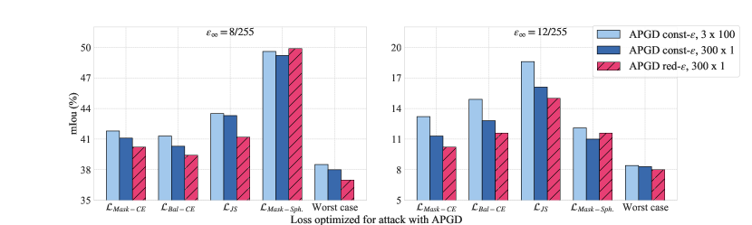
Figure 3: Testing difference between const-$\epsilon$ and red-$\epsilon$ schemes. Under the same iteration budget for the robust init. AT⁵ model, across different losses we see red-$\epsilon$ scheme leads to most drop in robust mIoU. Specifically for worst-case over all losses, red-$\epsilon$ leads to the best attack across different perturbation strengths.

Effect of reducing the radius. We complement the comparison of const-$\epsilon$ and red-$\epsilon$ schemes provided in Sec. 4.4 by showing the different robust mIoU achieved by the various algorithms. In Fig. 3 one can observe that, consistently with what reported for average accuracy in Fig. 2, reducing the value of $\epsilon$ (red-$\epsilon$ APGD) outperforms in most cases the other schemes.

Table 6: Component analysis for SEA. We show the individual performance of the runs of APGD with each loss in SEA. Additionally we include the worst-case over subsets of 3 out of 4 losses. We report robust average accuracy for robust models on both the datasets. The best results, among either individual runs or subgroups, are highlighted.

A:  $\mathcal{L}_{\textrm{Mask-CE}}$ + $\mathcal{L}_{\textrm{Bal-CE}}$ + $\mathcal{L}_{\textrm{JS}}$   B:  $\mathcal{L}_{\textrm{Mask-CE}}$ + $\mathcal{L}_{\textrm{Bal-CE}}$ + $\mathcal{L}_{\textrm{Mask-Sph.}}$   C:  $\mathcal{L}_{\textrm{Mask-CE}}$ + $\mathcal{L}_{\textrm{JS}}$ + $\mathcal{L}_{\textrm{Mask-Sph.}}$
$\epsilon_{\infty}$	individual losses				subsets of three losses			all
	$\mathcal{L}_{\textrm{Mask-CE}}$	$\mathcal{L}_{\textrm{Bal-CE}}$	$\mathcal{L}_{\textrm{JS}}$	$\mathcal{L}_{\textrm{Mask-Sph.}}$	A	B	C	(SEA)
model: AT5, robust init., 50 epochs, Pascal-Voc
4/255	89.0	88.5	88.4	90.5	88.3	88.5	88.4	88.3
8/255	73.7	72.9	73.8	80.7	71.6	71.7	71.8	71.3
12/255	31.6	35.9	38.6	38.1	29.4	27.4	27.8	27.3
16/255	6.7	11.9	12.5	6.8	5.8	4.3	4.3	4.2
model: AT5, robust init., 50 epochs, Ade20K
4/255	57.1	56.0	55.9	63.0	55.6	55.9	55.7	55.6
8/255	28.6	28.6	28.7	39.6	26.5	27.1	26.7	26.4
12/255	4.2	4.4	4.5	4.3	3.8	3.5	3.5	3.3

Contribution of individual components in SEA. To assess how much each loss contributes to the final performance of SEA, we report the individual performance (as average pixel accuracy after attack) at different $\epsilon_{\infty}$ in Table 6, using robust models on Pascal-Voc and Ade20K. We recall that each loss is optimized with 300 iterations of red-$\epsilon$ APGD. Additionally, we report the worst-case average pixel accuracy over subgroups of 3 out of 4 losses, and the worst-case of all 4, i.e. SEA. Although subset A works well for both datasets at $\epsilon_{\infty}\in\{4/255,8/255\}$, it is not as effective as subsets B and C for higher $\epsilon_{\infty}$, and vice-versa. Interestingly, $\mathcal{L}_{\textrm{Mask-Sph.}}$ does not yield the best individual results in any case, but the excluding it from the worst-case computation (subset A) significantly degrades the performance. Hence, the four losses have complementary properties, as observed in Sec. 4.3, which allows us to have effective attacks across the entire range of $\epsilon_{\infty}$.

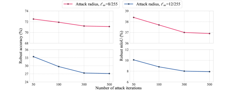
Figure 4: Influence of number of iterations in SEA. We show robust average accuracy (left) and mIoU (right) varying the number of iterations in our attack: 300 iterations give the best compute-effectiveness trade-off. We use the AT⁵ ConvNeXt-T backbone model with robust initialization for Pascal-Voc.

More iterations. We explore the effect of different number of iterations in SEA. In Fig. 4 we show the performance (measured by robust accuracy and mIoU) of SEA with 50, 100, 300 and 500 iterations. There is a substantial improvement going from 50 to 300 iterations in all cases. On further increasing the number of attack iterations to 500, the drop in robust accuracy and mIoU is around 0.1% for both $\ell_{\infty}$ radii of 8/255 and 12/255. Since going beyond 300 iterations gives no or minimal improvement for significantly higher computational cost, we fix the number of iterations to 300 in SEA.

Effect of random seed. We study the impact of the randomness involved in our algorithm (via random starting points for each run) by repeating the evaluation on our robust model on Pascal-Voc with 5 random seeds. Table 7 shows that the proposed SEA is very stable across all perturbation strengths. It is also interesting to note that all individual losses have negligible variance across the different runs.

Table 7: Stability of SEA across different runs. We report Acc computed on Pascal-Voc with the AT⁵ model. The mean across 5 runs is shown along with the standard deviation. Across all its components and perturbation strengths, SEA has a very low variance over random seeds.

A:  $\mathcal{L}_{\textrm{Mask-CE}}$ + $\mathcal{L}_{\textrm{Bal-CE}}$ + $\mathcal{L}_{\textrm{JS}}$   B:  $\mathcal{L}_{\textrm{Mask-CE}}$ + $\mathcal{L}_{\textrm{Bal-CE}}$ + $\mathcal{L}_{\textrm{Mask-Sph.}}$   C:  $\mathcal{L}_{\textrm{Mask-CE}}$ + $\mathcal{L}_{\textrm{JS}}$ + $\mathcal{L}_{\textrm{Mask-Sph.}}$
$\epsilon_{\infty}$	individual losses				subsets of three losses			all
	$\mathcal{L}_{\textrm{Mask-CE}}$	$\mathcal{L}_{\textrm{Bal-CE}}$	$\mathcal{L}_{\textrm{JS}}$	$\mathcal{L}_{\textrm{Mask-Sph.}}$	A	B	C	(SEA)
model: AT5, robust init., 50 epochs, Pascal-Voc
4/255	89.0 $\pm$ 0.1	88.5 $\pm$ 0.1	88.4 $\pm$ 0.1	90.5 $\pm$ 0.0	88.4 $\pm$ 0.1	88.5$\pm$ 0.0	88.4 $\pm$ 0.0	88.3 $\pm$ 0.0
8/255	73.6 $\pm$ 0.2	73.0 $\pm$ 0.3	73.7$\pm$ 0.1	80.6 $\pm$ 0.2	71.5$\pm$ 0.1	71.7$\pm$ 0.0	71.7$\pm$ 0.1	71.2$\pm$ 0.1
12/255	31.4$\pm$ 0.4	35.9$\pm$ 0.2	38.2$\pm$ 0.4	38.1$\pm$ 0.1	29.3 $\pm$ 0.2	27.6$\pm$ 0.2	27.9$\pm$ 0.1	27.3$\pm$ 0.1
16/255	6.6$\pm$ 0.1	11.9$\pm$ 0.3	12.3$\pm$ 0.2	6.9$\pm$ 0.1	5.7$\pm$ 0.1	4.3$\pm$ 0.1	4.3$\pm$ 0.1	4.2$\pm$ 0.1

C.2 Larger backbone for robust models

We test in this section the effect of using ConvNeXt-S, which is nearly 1.7x larger in terms of number of parameters than ConvNeXt-T considered until now, as backbone in UPerNet. We again take the $\ell_{\infty}=4/255$ robust ConvNeXt-S pre-trained on ImageNet from Singh et al. (2023) as initialization for our models. We note that this increases the size of the networks by only 1.4 times, since the backbone constitutes around 45% of it, while the FLOPs (in Giga) increase negligibly from 939 GFLOPs to 1027 GFLOPs. We keep the training setting consistent to ConvNeXt-T backbone models from the main text, see App. B.

In Table 8 we see that for Pascal-Voc the clean performance ($\epsilon_{\infty}=0$) of ConvNeXt-S backbone is better than ConvNeXt-T backbone models with the same training setup. The robustness for the model with AT² in mIoU is better by 2% on average, with smaller radii seeing larger improvements. For AT⁵, the increase of robust mIoU at $\epsilon_{\infty}=4/255$ is 3%, but for higher radii the improvement is only marginal if at all any. We hypothesize that the improvement could be much more if one increases the number of training epochs for these bigger models, as higher capacity needs more time to approach a better (robust) solution.

For Ade20K, clean performance gets slightly higher with the larger architectures. The improvement in robustness is around 2% (mIoU) for both $\epsilon_{\infty}=4/255$ and $\epsilon_{\infty}=8/255$, and around 0.6% for the largest radius. These results are consistent to what the original work introducing ConvNeXt showed when transitioning from ConvNeXt-T to ConvNeXt-S backbone. In fact, Liu et al. (2022) had a gain of 2.7% in clean mIoU which here translates to a slightly smaller improvement given we do adversarial training on top. In a similar vein, even large backbones could be tried and the increase in robustness would be tantamount to the increase from ConvNeXt-T to ConvNeXt-S, and we leave this to future work.

Table 8: Comparison of training schemes for Pascal-Voc and Ade20K with larger models. In continuation of Table 3 and Table 4, we show the effect of using a larger (robust) backbone, i.e. ConvNeXt-S, as initialization. The improvement in robustness (accuracy and mIoU) over ConvNeXt-T backbone for Pascal-Voc is marginal for small perturbations, whereas significant benefit can be seen for Ade20K across all perturbation strengths.

Training scheme			0		4/255		8/255		12/255		16/255
Pascal-Voc
ConvNeXt-T backbone
AT2	robust init.	50 ep.	92.9	75.9	86.7	60.8	50.2	21.0	9.3	2.4	0.8	0.3
AT5	robust init.	50 ep.	92.7	75.2	88.3	63.8	71.2	37.0	27.4	8.1	4.2	0.9
ConvNeXt-S backbone
AT2	robust init.	50 ep.	93.4	77.2	87.8	63.2	53.5	23.0	10.3	2.7	0.9	0.4
AT5	robust init.	50 ep.	93.1	76.6	89.2	66.2	70.8	38.0	27.0	8.6	3.9	1.0
Ade20K
ConvNeXt-T backbone
AT5	robust init.	128 ep.	70.5	31.7	55.6	18.6	26.4	6.7	3.3	0.8	–	–
ConvNeXt-S backbone
AT5	robust init.	128 ep.	71.3	32.1	57.2	19.2	28.8	7.2	3.9	0.9	–	–

Table 9: Comparison of training schemes for an additional segmentation architecture. Segmenter (Strudel et al., 2021) is a recently proposed architecture with Vision Transformer (ViT-S) as backbone. For Ade20K we notice that for Segmenter, the robust initialized model is more robust at all perturbation strengths than its clean initialized counterpart, similar to the trend for UPerNet.

Training scheme			0		4/255		8/255		12/255
clean		128 ep.	74.3	39.4	0.0	0.0	0.0	0.0	0.0	0.0
AT5	clean init.	128 ep.	67.7	26.8	48.4	12.6	25.0	4.7	4.5	0.8
AT5	robust init.	128 ep.	69.1	28.7	54.5	16.5	31.0	7.1	6.8	1.6

C.3 Excluding the background class from evaluation

For Ade20K, we train clean models in two settings, i.e. either ignoring the background class (150 possible classes), which is the standard practice while training clean semantic segmentation models, or to predict it (151 classes). To measure the effect of the additional background class, we can evaluate the performance of both models with only 150 classes (for the one trained on 151 classes, we can exclude the score of the background class when computing the predictions). Training on 150 classes achieves (Acc, mIoU) of (80.4%, 43.8%), compared to (80.2%, 43.8%) for 151. This shows that we do not lose any performance when training with the background class, and the apparent lower results reported e.g. in Table 4, (Acc, mIoU) of (75.5%, 41.1%) are due to including the background class when computing the statistics. This also translates to the robust models trained in the AT² setting. For the robust model, the two settings have (76.6%, 37.8%) and (76.4%, 37.5%) (Acc, mIoU) respectively.

C.4 Additional segmentation architectures

In this section, we test if the effectiveness of using ImageNet robust classifiers as backbone for UPerNet translates to other segmentation architectures. To this end, we consider Segmenter (Strudel et al., 2021) an encoder-decoder architecture similar to UPerNet but designed for Vision Transformers (ViT) (Dosovitskiy et al., 2020) as backbone (encoder). Testing with Segmenter also enables a further comparison across model size as Segmenter with a ViT-S backbone is less than half the size (26 million parameters) of UPerNet with a ConvNeXt-T backbone (60 million parameters). We use the ViT-S adversarially trained on ImageNet from Singh et al. (2023) as robust initialization, and the ViT-S trained only on ImageNet-1k from timm library. The decoder is a Mask transformer and is randomly initialized. Note that in the original Segmenter work Strudel et al. (2021) predominantly use ImageNet pre-trained classifiers at resolution of 384x384, whereas we use 224x224 resolution as no robust models at resolution of 384x384 are available. We stay consistent with the original training setting (for 160k total updates with SGD as optimizer) as proposed by Strudel et al. (2021) with only changes being the batch size set to 16x8 and learning rate doubled to 2e-3.

In Table 9, we report the results of Segmenter models on Ade20K for various training setting (clean and AT⁵, i.e. adversarial training with 5 steps of PGD). We see that, across perturbation strengths, the robust ViT backbone leads to a more robust segmentation model, which is consistent to the earlier findings for UPerNet. The difference in both Acc and mIoU from clean to robust initialization is even larger than for UPerNet with a ConvNeXt backbone, see Table 4. The robustness is again tested with the proposed SEA attack.

Appendix D Additional Figures

Untargeted attacks. Fig. 5 shows examples of our untargeted attacks at different radii $\epsilon_{\infty}$ on the clean model for Pascal-Voc dataset. In particular, we use 300 iterations of red-$\epsilon$ APGD on the $\mathcal{L}_{\textrm{Mask-CE}}$ loss. The first column presents the original image with the ground truth segmentation mask, The following columns contain the perturbed images and relative predicted segmentation masks for increasing radii ($\epsilon_{\infty}=0$ is equivalent to the unperturbed image): one can observe that the model predictions progressively become farther away from the ground truth values. We additionally report the average pixel accuracy for each image. In Fig. 6, we repeat the same visualization for AT⁵ model with robust initialization. Note that we use different values of $\epsilon_{\infty}$ for the two models, i.e. significantly smaller ones for the clean model, following Table 2. Finally, the same setup is employed on the Ade20K dataset for the illustrations in Fig. 7 (clean model) and Fig. 8 (robust model), and we have similar observations as for the smaller dataset. Again we use smaller radii for the clean model, since it is significantly less robust than the AT⁵ one.

Targeted attacks. In Fig. 1 we show examples of the perturbed images and corresponding predictions resulting from targeted attacks. In this case, we run APGD (red-$\epsilon$ scheme with 300 iterations) on the negative JS divergence between the model predictions and the one-hot encoding of the target class. In this way the algorithm optimizes the adversarial perturbation to have all pixels classified in the target class (e.g. “grass” or “sky” in Fig. 1). We note that other losses like cross-entropy can be adapted to obtain a targeted version of SEA, and we leave the exploration of this aspect of our attacks to future work.

original	0	0.25/255	0.5/255	1/255	2/255
	Acc: 95.9%	Acc: 94.8%	Acc: 75.9%	Acc: 48.3%	Acc: 0.0%
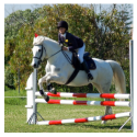
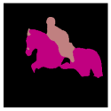
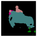
	Acc: 96.1%	Acc: 61.4%	Acc: 0.0%	Acc: 0.0%	Acc: 0.0%

Figure 5: We show the perturbed images, corresponding predicted segmentation masks and average accuracy for increasing radii. The attacks are generated on the clean model on Pascal-Voc with APGD on $\mathcal{L}_{\textrm{Mask-CE}}$. We additionally present (first column) the original image and ground truth mask.

original	0	4/255	8/255	12/255	16/255
	Acc: 95.5%	Acc: 94.6%	Acc: 90.8%	Acc: 49.2%	Acc: 0.0%
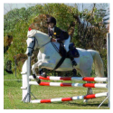
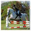
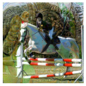
	Acc: 93.7%	Acc: 92.7%	Acc: 83.3%	Acc: 6.8%	Acc: 0.0%

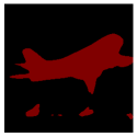
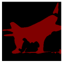
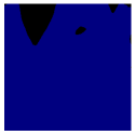
Figure 6: Same setting as in Fig. 5 for the robust AT⁵ model. Note the larger radii $\epsilon$ for the attack.

original	0	0.25/255	0.5/255	1/255	2/255
	Acc: 65.9%	Acc: 54.9%	Acc: 4.9%	Acc: 0.0%	Acc: 0.0%
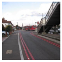
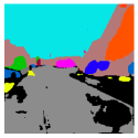
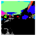
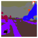
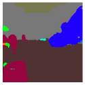
	Acc: 81.2%	Acc: 47.9%	Acc: 21.9%	Acc: 2.6%	Acc: 0.0%

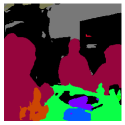
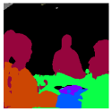
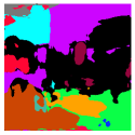
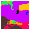
Figure 7: We show the perturbed images, corresponding predicted segmentation masks and average accuracy for increasing radii. The attacks are generated on the clean model on Ade20K with APGD on $\mathcal{L}_{\textrm{Mask-CE}}$. We additionally present (first column) the original image and ground truth mask.

original	0	4/255	8/255	12/255	16/255
	Acc: 61.3%	Acc: 58.6%	Acc: 29.7%	Acc: 1.6%	Acc: 0.0%
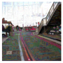
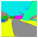
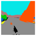
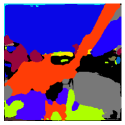
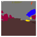
	Acc: 84.4%	Acc: 67.3%	Acc: 32.8%	Acc: 6.0%	Acc: 0.0%

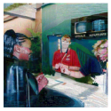
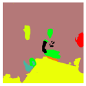
Figure 8: Same setting as in Fig. 7 for the robust AT⁵ model. Note the larger radii $\epsilon$ for the attack.