Control of Spin Polarization through Recollisions

Abstract

Using only linearly polarized light, we study the possibility of generating spin-polarized photoelectrons from xenon atoms. No net spin polarization is possible, since the xenon ground state is spin-less, but when the photoelectron are measured in coincidence with the residual ion, spin polarization emerges. Furthermore, we show that ultrafast dynamics of the recolliding photoelectrons contribute to an apparent flipping of the spin of the photoelectron, a process that has been completely neglected so far in all analyses of recollision-based processes. We link this phenomenon to the “spin–orbit clock” of the remaining ion. These effects arise already in dipole approximation.

Published in

Physical Review A 108(4), 043104 (2023), DOI: 10.1103/PhysRevA.108.043104

I Introduction

Generation of spin-polarized photoelectrons using intense circularly polarized light has recently become a topic of great interest [1, 2, 3, 4, 5]. Since the rare gases commonly employed in strong-field ionization experiments are spin-less in the ground state, linearly polarized light cannot generate net spin polarization. In this article we show that when the photoelectron is measured in coincidence with the final ion state, the spin polarization approaches $100\text{\,}\mathrm{\char 37\relax}\text{/}$ in the individual ionization channels (resolved on $J$ and $M_{J}$). Furthermore, we link the resulting spin polarization to the rescattering electron imaging the ultrafast hole motion, providing an intuitive picture of electron trajectories that contribute to an apparent spin flip of the detected electron — a signature of recollision-driven coupling between continua with different spins. We find that the spin-flip recollisions are very significant, and that we may exercise precise control over the outcome. This effect, which has so far been overlooked, is important in all recollision-based imaging techniques such as laser-induced electron diffraction [6], electron holography [7], and orbital tomography [8, 9].

This article is arranged as follows: section II introduces the computational tools we employ in the calculations, presented in section III. Section IV concludes the article.

II Theory

Our method consistently treats multi-electron spin dynamics in strong laser fields, and is thus suitable for our chosen target, xenon. It is based upon the time-dependent configuration-interaction singles (TD-CIS) [10, 11, 12, *Carlstroem2022tdcisII]. The equations of motion (EOMs) describe the time evolution of the amplitude $c_{0}$ for the Hartree–Fock (HF) reference state, and the particle orbital $\ket*{\tilde{k}}$ emanating from the initially occupied (time-independent) orbital $\ket{k}$. Below, we employ Hartree atomic units. Quantities appearing on one side only are summed/integrated over. The different particle–hole channels can couple via both the laser interaction and the Coulomb interaction:

$$\mathrm{i}\partial_{t}c_{0} ={\matrixelement*{k}{\hat{V}_{L}}{\tilde{k}}},$$ (1)

$$\mathrm{i}\partial_{t}\ket*{\tilde{k}} =(-\epsilon_{k}+{\hat{f}})\ket*{\tilde{k}}+{c_{0}\hat{V}_{L}\ket{k}}-{\matrixelement{l}{\hat{V}_{L}}{k}}\ket*{\tilde{l}}$$

$$\hphantom{=}-{(\hat{J}_{lk}-\hat{K}_{lk})\ket*{\tilde{l}}}-\lambda_{\tilde{k}m}\ket{m},$$

where $\epsilon_{k}$ is the eigenvalue of the initially occupied orbital $\ket{k}$. The Fock operator is defined as $\hat{f}\overset{\textrm{\tiny def}}{=}\hat{h}+\hat{J}_{mm}-\hat{K}_{mm}$, with the one-body Hamiltonian containing the interaction with the external laser field, $\hat{h}\overset{\textrm{\tiny def}}{=}p^{2}/2+\hat{V}_{C}(\bm{r})+\hat{V}_{L}$, $\hat{V}_{L}\overset{\textrm{\tiny def}}{=}\bm{F}(t)\cdot\bm{r}$, and $\hat{J}_{cd}$ and $\hat{K}_{cd}$ are the direct and exchange interaction potentials, respectively (see Appendix A.1). The Lagrange multipliers $\lambda_{\tilde{k}m}$ in Equation (1) ensure that $\ket*{\tilde{k}}$ at all times remains orthogonal to all initially occupied orbitals $\ket{m}$.

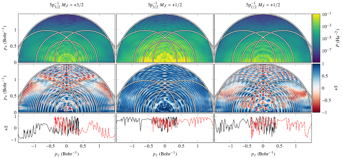
Figure 1: Top row: Angularly resolved ATI spectra from xenon, correlated to different ionic channels. Middle row: Spin polarization of the photoelectrons; for $M_{J}<0$, the spin polarization is exactly the opposite of the positive case. Blue colour means excess of spin-up (spin-down) for $+S$ ($-S$), and vice versa for red. The overlaid concentric circles indicate momenta at the detector corresponding to kinetic energies $2U_{\mathrm{p}}$, $4U_{\mathrm{p}}$, $10U_{\mathrm{p}}$, respectively. The offset circles mark the contribution of recolliding electrons with the maximum possible return energy $W_{k,\textrm{max}}$. Bottom row: Lineouts along the $W_{k,\textrm{max}}$ circles in the middle row; the black solid (red dashed) line corresponds to initial ionization towards positive (negative) $p_{z}$.

To implement spin–orbit coupling, instead of resorting to the full four-component Dirac–Fock treatment (RTDCIS [14]), we rely on the phenomenological two-component treatment of Peterson et al. [15]. It includes corrections due to scalar-relativistic effects, and at the same time reduces the number of electrons we need to treat explicitly. It replaces the scalar potential $\hat{V}_{C}$ by the relativistic effective core potential (RECP), which models the atomic nucleus and the 1s–3d electrons of xenon according to

$$\hat{V}^{\textrm{RECP}}(\bm{r})=\hat{V}^{\textrm{scalar}}(r)+\mu\hat{V}^{\textrm{s--o}}_{\ell j}(r).$$ (2)

The RECP allows us to identify effects associated with spin–orbit dynamics by scaling the spin–orbit splitting as

$$\Delta E_{\textrm{s--o}}(\mu)\approx\mu\Delta E_{\textrm{s--o}}(1),$$ (3)

where $\Delta E_{\textrm{s--o}}(1)\approx$1.4\text{\,}\mathrm{eV}\text{/}$$ is the nominal spin–orbit splitting of the ionic ground state at the CIS level; the dependence is essentially linear in $\mu$ (see Appendix A.2).

The spin polarization is given by

$$S_{I}(E,\theta)\overset{\textrm{\tiny def}}{=}\frac{P_{I\alpha}(E,\theta)-P_{I\beta}(E,\theta)}{P_{I\alpha}(E,\theta)+P_{I\beta}(E,\theta)},$$

where $P_{I{\sigma_{z}}}(E,\theta)$ is the ion-, kinetic energy-, angle-, and spin-resolved photoelectron distribution (see Appendix A.3).

III Calculations

We study above-threshold ionization (ATI) from xenon, with the following ionization channels included: ${\mathrm{5p}}^{-1}_{3/2}$, $M_{J}=\pm 3/2,\pm 1/2$, and ${\mathrm{5p}}^{-1}_{1/2}$, $M_{J}=\pm 1/2$ . Ionization from $\mathrm{5s}$ and lower-lying orbitals is strongly suppressed in the laser fields we consider [$\hbar\omega=\Delta E_{\textrm{s--o}}(1)$ and $I_{0}=$44\text{\,}\mathrm{TW}\text{/}{\mathrm{cm}}^{2}$$]. The spin-mixed channels ${\mathrm{5p}}^{-1}_{3/2}$, $M_{J}=\pm 1/2$ (formed from linear combinations of $\mathrm{p}_{0}\alpha$, $\mathrm{p}_{+}\beta$ and $\mathrm{p}_{0}\beta$, $\mathrm{p}_{-}\alpha$, respectively) are preferentially ionized, since ionization in linearly polarized fields is dominated by $\mathrm{p}_{0}$ [17].

The weaker channels ${\mathrm{5p}}^{-1}_{3/2}$, $M_{J}=\pm 3/2$ are expected to be spin-pure, since to form the orbitals $\mathrm{5p}_{3/2}$, $m_{j}=\pm 3/2$, the orbital- and spin-angular momenta must be maximally aligned ($\mathrm{p}_{+}\alpha$ and $\mathrm{p}_{-}\beta$, respectively). Linearly polarized electric fields preserve spin, and thus we expect that the outgoing electron is spin-pure as well. However, the results of our numerical simulations are surprising: only direct, on-axis photoelectrons maintain their expected spin (see Figure 1). In contrast electrons that have undergone recollision with the parent ion, and are able to travel off-axis, exhibit substantial amounts of the opposite spin.

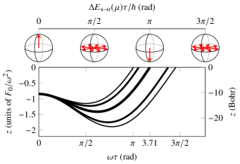
Figure 2: Sketch of the proposed spin-flipping mechanism; the electron moves along a rescattering trajectory with an excursion phase of $\omega\tau$, which in the example is chosen such that the trajectory with maximum return energy $W_{k,\textrm{max}}$, shown as the heaviest line, matches half a revolution of the spin–orbit clock, illustrated as Bloch spheres. The classical trajectories start at the tunnel exit of a Coulombic barrier.

To explain this behaviour, we posit that this effect results from the recollision of the returning electron off of the ion, which in the spin-mixed channels has time-evolving spin [1, 5]. Directly after ionization, the ion has a spin opposite that of the photoelectron, yielding vanishing spin overall. If upon return, the electron finds an ion with a spin different from that at time of ionization, inelastic scattering into the spin-pure channels ${\mathrm{5p}}^{-1}_{3/2}$, $M_{J}=\pm 3/2$ may contribute to photoelectrons of opposite spin in these channels. Furthermore, this apparent spin flip will predominantly occur when $\Delta E_{\textrm{s--o}}\tau\approx\pi$, where $\tau$ is the excursion time of the electron, see Figure 2 and the SI (see Appendix B). This dynamic corresponds to the spin–orbit clock in the ion undergoing half a revolution.

To investigate this hypothesis in a minimally invasive manner, we tune the spin–orbit splitting $\Delta E_{\textrm{s--o}}$ by changing the value of $\mu$ in (2), while keeping all remaining parameters constant. We then find

$$\pi\approx\Delta E_{\textrm{s--o}}(\mu)\tau=\frac{\Delta E_{\textrm{s--o}}(\mu)}{\omega}\omega\tau=\frac{\Delta E_{\textrm{s--o}}(\mu)}{\Delta E_{\textrm{s--o}}(1)}\omega\tau,$$ (4)

since we chose the photon energy to be in resonance with the nominal spin–orbit splitting, $\omega=\Delta E_{\textrm{s--o}}(1)$. Using (3), we get

$$\mu\approx\frac{\Delta E_{\textrm{s--o}}(\mu)}{\Delta E_{\textrm{s--o}}(1)}\approx\frac{\pi}{\omega\tau}.$$ (5)

For electrons returning with maximal kinetic energy, $W_{k,\textrm{max}}$, which return at $\omega\tau\approx 3.71$, we obtain $\mu\approx 0.85$. It is easy to find those final momenta (combinations of $p_{z}$ and $p_{x}$) which result from trajectories recolliding with $W_{k,\textrm{max}}$ [18] (see Appendix B); these are marked in Figure 1 with circles in the forward ($p_{z}>0$) and backward ($p_{z}<0$) directions. If we take lineouts of the spin polarization along these circles, we predominantly measure the contribution of trajectories returning with $W_{k,\textrm{max}}$ kinetic energy. The red streaks in Figure 1 that indicate the opposite spin do not fall perfectly on the $W_{k,\textrm{max}}$ circle; this is mostly due to the circle being derived for classical trajectories with no potential present. The slight shift in momentum for the apparent spin flips is a result of Coulomb focusing.

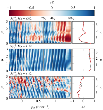
Figure 3: Lineouts along the $W_{k,\textrm{max}}$ circles in Figure 1, for a range of values of the spin–orbit scaling parameter $\mu$ [see Equation (3)], plotted as a function of $p_{z}$; note that $2W_{k}=p_{z}^{2}+p_{x}^{2}$, and the lineouts are not taken along constant $p_{x}$. As in Figure 1, for $M_{J}<0$, the spin polarization is exactly $-S$. Each row corresponds to a specific ion channel; top row the spin-pure channel ${\mathrm{5p}}^{-1}_{3/2}$, $M_{J}=+3/2$, middle row ${\mathrm{5p}}^{-1}_{3/2}$, $M_{J}=+1/2$, bottom row ${\mathrm{5p}}^{-1}_{1/2}$, $M_{J}=+1/2$. The left column shows emission in the forward direction, i.e. positive final $p_{z}$ [due to the long pulse duration, $\tau=$15\text{\,}\mathrm{fs}\text{/}$$, the spin polarization is almost symmetric about $p_{z}=0$ (see Appendix B.1)]. The right column shows the integrated spin polarization along the lineout, from $p^{2}/2=4U_{\mathrm{p}}$ to $p_{\textrm{max}}$; the solid, black line corresponds to the forward emission, and the dashed red to the backward emission. The right ordinate indicate the expected positions corresponding to $n\approx\mu\omega\tau/\pi$ half-revolutions of the spin–orbit clock, for $\omega\tau\approx 3.71$ (see main text).

We thus expect large amounts of opposite spin in the high-rescattering region ($\left|W_{k}\right|>4U_{\mathrm{p}}$), for $\mu\approx 0.85$, since the spin–orbit clock has undergone half a revolution, by the time electron returns. In Figure 3 we see that this is indeed the case, in the spin-pure channels ${\mathrm{5p}}^{-1}_{3/2}$, $M_{J}=\pm 3/2$. Generalizing this argument, for $\mu\approx\frac{n\pi}{\omega\tau}=0.85,1.69,2.54,3.40,4.23,5.07,...$ we expect to see enhancement and suppression of the opposite spin for odd $n$ and even $n$, respectively.

It is also interesting to note that for $\mu=0$, the photoelectrons in the spin-pure channel are spin-pure as well. In this case, the period of the spin–orbit clock is $\frac{2\pi}{\Delta E_{\textrm{s--o}}(0^{+})}=+\infty$, and the hole remains forever in its initial spin state, preventing any opposite spin appearing in the spin-pure channels.

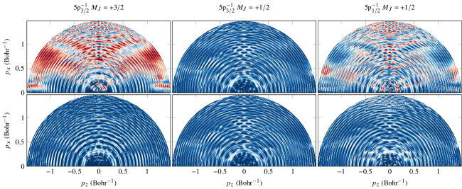
Figure 4: Effect on the spin polarization when gradually removing the Coulomb electron–electron repulsion interaction from the EOMs (1). Top row: $\hat{K}_{lk}$ dropped; bottom row; $\hat{K}_{lk},\hat{J}_{lk}$ dropped. See the second row of Figure 1 for the case where all terms in the Hamiltonian are included.

To further explore the proposed mechanism, we selectively remove the Coulomb repulsion interaction from the EOMs (1); first we exclude exchange-type interactions between ionization channels by dropping the $\hat{K}_{lk}$ term, and then the direct-type interchannel interactions $\hat{J}_{lk}$. Dropping the self-interaction correction $\hat{K}_{mm}$ does not influence the spin polarization appreciably (see Appendix C.1). The intrachannel interactions $\hat{J}_{mm}$ must remain, since otherwise the problem would reduce to a hydrogenic one with a bare xenon nucleus. We compare these instrumented calculations with the full Hamiltonian in Figure 4. As we see in the figure, the largest effect is the removal of $\hat{J}_{lk}$, which is the only term of the three which is long-range ($\hat{K}$, being traceless, decays at least as quickly as $r^{-2}$). We also note that the removal of $\hat{K}_{lk}$ quantitatively changes the angular distribution of the spin polarization, even enhancing it, which suggests that $\hat{K}_{lk}$ actually works counter to the proposed mechanism.

We now understand the mechanism leading to the opposite spin in the spin-pure channel better: The hole in this channel is also spin-pure, and as such does not undergo any spin oscillation in the spin–orbit clock. However, the holes in the other channels are spin-mixed, and the spin–orbit clock oscillates with the period $T_{\textrm{s--o}}\overset{\textrm{\tiny def}}{=}\frac{2\pi}{\Delta E_{\textrm{s--o}}(\mu)}$. After rescattering at the right moment, we may observe opposite spins due to inelastic scattering into ${\mathrm{5p}}^{-1}_{3/2}$, $M_{J}=\pm 3/2$. Removing $\hat{J}_{lk}$ from the EOMs (1) suppresses inelastic scattering, and thus precludes any transfer of spin between channels, as we see in Figure 4. This mechanism can be semi-quantitatively investigated by considering the explicit time–spin dependence of $\hat{J}_{lk}$ and $\hat{K}_{lk}$ in $LS$ coupling, where the orbitals $l$ and $k$ change their spin with the period $T_{\textrm{s--o}}$ (see Appendix C.2).

IV Conclusions

In conclusion, we have demonstrated that we can generate spin-polarized electrons, even when ionizing using linearly polarized light, as long as we detect the photoelectrons in coincidence with the ion. Furthermore, due to the recollision mechanism in strong-field ionization, we are also able to control the spin of the photoelectron, by tuning the ratio of the spin–orbit splitting and the angular frequency of the driving field. This mechanism has important implications for recollision-based imaging techniques such as laser-induced electron diffraction, which use the energy– and angle-resolved distribution of the photoelectron to infer the state of the ion; through the spin–orbit interaction, the spin of the photoelectron would reveal additional information on the entangled photoion.

Appendix A Methods

A.1 Coulomb Repulsion

The direct and exchange interaction potentials are defined by their action on a spin-orbital

$$\hat{J}_{cd}\ket{e} \overset{\textrm{\tiny def}}{=}\chi_{e}(\varsigma_{1})\int\frac{\mathrm{d}\varsigma_{2}}{\left|\bm{r}_{1}-\bm{r}_{2}\right|}\chi_{c}^{*}(\varsigma_{2})\chi_{d}(\varsigma_{2}),$$ (6)

$$\hat{K}_{cd}\ket{e} \overset{\textrm{\tiny def}}{=}\chi_{d}(\varsigma_{1})\int\frac{\mathrm{d}\varsigma_{2}}{\left|\bm{r}_{1}-\bm{r}_{2}\right|}\chi_{c}^{*}(\varsigma_{2})\chi_{e}(\varsigma_{2})\equiv\hat{J}_{ce}\ket{d},$$

where $\varsigma_{1,2}$ refer to both the spatial and spin coordinates.

A.2 Scaling the Spin–Orbit Interaction

The explicit form of the RECP (2) is

$$\hat{V}^{\textrm{RECP}}(\bm{r}) =\hat{V}^{\textrm{scalar}}(r)+\mu\hat{V}^{\textrm{s--o}}_{\ell j}(r),$$ (7)

$$\hat{V}^{\textrm{scalar}}(r) \overset{\textrm{\tiny def}}{=}-\frac{Q}{r}+\hat{V}_{\ell}(r)\hat{P}_{\ell},$$

$$\hat{V}_{\ell}(r) \overset{\textrm{\tiny def}}{=}\frac{1}{2\ell+1}[\ell\hat{V}_{\ell,\left|\ell-\frac{1}{2}\right|}(r)+(\ell+1)\hat{V}_{\ell,\ell+\frac{1}{2}}(r)],$$

$$\hat{P}_{\ell} \overset{\textrm{\tiny def}}{=}\hat{P}_{\ell,\left|\ell-\frac{1}{2}\right|}+\hat{P}_{\ell,\ell+\frac{1}{2}},$$

$$\hat{V}^{\textrm{s--o}}_{\ell j}(r) \overset{\textrm{\tiny def}}{=}\frac{\Delta\hat{V}_{\ell}(r)}{2\ell+2}[\ell\hat{P}_{\ell,\ell+1/2}-(\ell+1)\hat{P}_{\ell,\ell-1/2}],$$

$$\Delta\hat{V}_{\ell}(r) \overset{\textrm{\tiny def}}{=}\hat{V}_{\ell,\ell+1/2}(r)-\hat{V}_{\ell,\ell-1/2}(r),$$

$$\hat{V}_{\ell j} \overset{\textrm{\tiny def}}{=}B_{\ell j}^{k}\exp(-\beta_{\ell j}^{k}r^{2}),$$

where $Q=26$ is the residual charge, $\hat{P}_{\ell j}$ is a projector on the spin–angular symmetry $\ell j$, and $B_{\ell j}^{k}$ and $\beta_{\ell j}^{k}$ are numeric coefficients found by fitting to multiconfigurational Dirac–Fock all-electron calculations of the excited spectrum [19, 20].

In Figure 5, we show the effect of scaling the spin–orbit interaction in the RECP (7). The resultant spin–orbit splitting is essentially proportional to $\mu$. In Table 1, the calculated ionization potentials for the case $\mu=1$ are compared with experimental values from the literature.

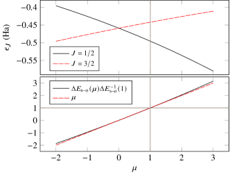
Figure 5: Spin–orbit splitting $\Delta E_{\textrm{s--o}}(\mu)\overset{\textrm{\tiny def}}{=}\epsilon_{3/2}(\mu)-\epsilon_{1/2}(\mu)$ between ${\mathrm{5p}}^{-1}_{3/2}$ and ${\mathrm{5p}}^{-1}_{1/2}$, as a function of the scaling parameter $\mu$ in Equation (2).

Table 1: Calculated ionization potentials of the $5\mathrm{s}$, $\mathrm{5p}$ electrons of xenon, compared with their experimental and RCIS values (Refs: [21]${}^{\textrm{a}}$, [22]${}^{\textrm{b}}$, [14]${}^{\textrm{c}}$).

Hole	$I_{\mathrm{p}}$ ($\mathrm{eV}\text{/}$)	Exp. ($\mathrm{eV}\text{/}$)	$\Delta$ ($\mathrm{eV}\text{/}$)	RCIS $I_{\mathrm{p}}$ ($\mathrm{eV}\text{/}$)
${\mathrm{5p}}^{-1}_{3/2}$	$12.026$	$12.130$${}^{\textrm{a}}$	$-0.104$	$11.968$${}^{\textrm{c}}$
${\mathrm{5p}}^{-1}_{1/2}$	$13.483$	$13.436$${}^{\textrm{b}}$	$0.047$	$13.404$${}^{\textrm{c}}$
${\mathrm{5s}}^{-1}_{1/2}$	$27.927$	$23.397$${}^{\textrm{b}}$	$4.530$	$27.485$${}^{\textrm{c}}$

A.3 Photoelectron Spectra

The photoelectron distributions, resolved on ion state $I$, photoelectron energy $E$, the angle $\theta$ with respect to the polarization axis, and with spin projection ${\sigma_{z}}$, are obtained by tracing over the reduced density matrix:

$$P_{I{\sigma_{z}}}(E,\theta)\overset{\textrm{\tiny def}}{=}\int\mathrm{d}\phi\matrixelement{{\sigma_{z}}}{\hat{\rho}_{II}(E,\theta,\phi)}{{\sigma_{z}}}.$$ (8)

The density matrix is formed from the outer product of the wavefunction with itself,

$$\hat{\rho}(E,\theta,\phi)\overset{\textrm{\tiny def}}{=}\outerproduct{\Psi(\bm{k})}{\Psi(\bm{k})},$$ (9)

using the close-coupling Ansatz [23] for the wavefunction

$$\ket{\Psi(\bm{k})}=c_{I\bm{k}{\sigma_{z}}}\mathcal{A}\ket{I}\ket{\bm{k}{\sigma_{z}}}$$ (10)

where $\ket{I}$ is the state of the ion,

$$\bm{k}=\begin{bmatrix}k\sin\theta\cos\phi\\ k\sin\theta\sin\phi\\ k\cos\theta\end{bmatrix},\quad k=\sqrt{2E},$$

is the asymptotic momentum of the photoelectron, ${\sigma_{z}}$ the spin projection of the photoelectron, and $\mathcal{A}$ the antisymmetrization operator. The reduced density matrix is obtained from the full density matrix, by projecting on specific ion states:

$$\hat{\rho}_{IJ}\overset{\textrm{\tiny def}}{=}\matrixelement{I}{\hat{\rho}}{J}.$$ (11)

The decomposition (10) is computed [12, *Carlstroem2022tdcisII] using the tSURFF [24, 25, 26, 27, 28] and iSURFV [29] techniques.

Appendix B Classical Trajectories

Here we re-derive the classical trajectories of a free electron in a monochromatic electric field

$$\bm{F}(t)=\bm{F}_{0}\cos(\omega t);$$

these results have been presented many times, most notably by Corkum [30].

We introduce the free oscillation range and the velocity amplitude:

$$\bm{\alpha}\overset{\textrm{\tiny def}}{=}\frac{\bm{F}_{0}}{\omega^{2}};\qquad\bm{v}_{0}\overset{\textrm{\tiny def}}{=}\frac{\bm{F}_{0}}{\omega};$$

(we note that $v_{0}^{2}=4U_{\mathrm{p}}$), as well as the phases $\phi=\omega t$, $\phi_{i}=\omega t_{i}$, and $\phi_{r}=\omega t_{r}$, $\delta\phi=\phi_{r}-\phi_{i}\equiv\omega\tau$, etc.

We find the trajectories by integrating Newton’s equations $\bm{a}(t)=-\bm{F}(t)$, neglecting the influence of the atomic potential:

$$\bm{v}(t)=-\bm{F}_{0}\int_{t_{i}}^{t}\mathrm{d}t^{\prime}\cos\phi^{\prime}=-\bm{v}_{0}(\sin\phi-\sin\phi_{i}),$$

$$\bm{r}(t) =\bm{r}_{0}+\bm{\alpha}[\cos\phi-\cos\phi_{i}+(\phi-\phi_{i})\sin\phi_{i}].$$

The phase of ionization $\phi_{i}$ is found for each rescattering phase $\phi_{r}$ by requiring that the electron returns to the origin before rescattering:

$$\bm{r}(t_{r})=0,$$

which we solve numerically using the gradient method.

The kinetic energy of the electron (before rescattering) is given by

$$W_{k}(t)=\frac{v^{2}(t)}{2}\equiv 2U_{\mathrm{p}}(\sin\phi-\sin\phi_{i})^{2}.$$ (12)

Table 2: Influence of the initial position on the maximal kinetic energy upon rescattering, for $F_{0}=$3.5408\text{\times}{10}^{-2}\text{\,}\mathrm{a}\mathrm{u}$$ and $\omega=$0.0535\text{\,}\mathrm{Ha}\text{/}$$.

Barrier	$r_{0}$ (Bohr)	$W_{k,\textrm{max}}$ ($U_{\mathrm{p}}$)	$\phi_{i}$ (rad)	$\phi_{r}$ (rad)	$\delta\phi$ (rad)
None	$0.0$	$3.17$	$0.31$	$4.40$	$4.08$
Triangular	$-12.96$	$4.69$	$0.68$	$4.27$	$3.59$
Coulomb	$-10.49$	$4.36$	$0.59$	$4.30$	$3.71$

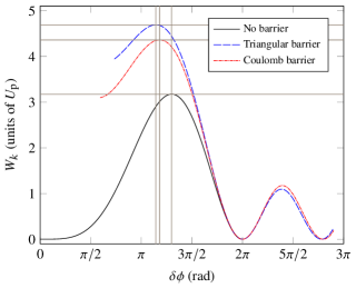
Figure 6: Kinetic energy upon rescattering as function of excursion phase, for three different choices of initial starting position (given in Table 2).

We may choose the initial position at the tunnel exit

$$r_{0}^{\textrm{tri}} =-\frac{I_{\mathrm{p}}missing}{F_{0}},$$ or (13)

$$r_{0}^{\textrm{Coul}} =-\frac{I_{\mathrm{p}}missing}{2F_{0}}-\sqrt{\left(\frac{I_{\mathrm{p}}missing}{2F_{0}}\right)^{2}-\frac{2I_{\mathrm{p}}missing}{F_{0}}},$$

which will give maximal kinetic energies at the time of rescattering, rather different from when the electron starts at the origin $r_{0}=0$ (see Table 2 and Figure 6), and in turn influence the final momenta on the detector which upon rescattering had the maximal kinetic energy (see Figure 7). Accounting for the initial position is an important improvement compared to starting at the origin as done by Spanner et al. [18], since it allows us to correctly sample the off-axis spin-flip features as seen in Figure 1 of the main text; for the figures shown there, we use the initial position $r_{0}^{\textrm{Coul}}$ for a Coulombic barrier.

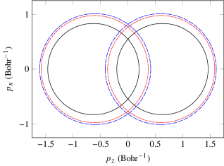
Figure 7: Final electron momenta corresponding to maximal kinetic energy upon rescattering, for three different choices of initial starting position (line patterns are the same as in Figure 6).

B.1 Lineouts in the Backward Emission Direction

In Figure 8, the lineouts along the $W_{k,\textrm{max}}$ circles in the backward emission direction are shown. Due to the long pulse duration ($\tau=$15\text{\,}\mathrm{fs}\text{/}$$), the spin polarization in the backward direction is almost a perfect mirror image of the forward distribution, as evidenced by the similarity of the integrated lineouts also shown in the figure.

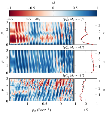
Figure 8: Similar to Figure 3 of the main manuscript, but the lineouts are instead along the $W_{k,\textrm{max}}$ circles in the backward direction, i.e. negative final $p_{z}$.

Appendix C Scattering Matrix Elements

C.1 Effect of Removing $\hat{K}_{mm}$

See Figure 9 for the effect of removing $\hat{K}_{mm}$ from the EOMs; the results do not change appreciably.

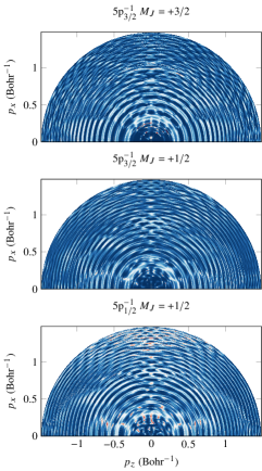
Figure 9: The effect of removing $\hat{K}_{mm}$ from the EOMs does not appreciably affect the spin-flipping mechanism; cf. Figure 4 of the main manuscript.

C.2 Time-Dependent Scattering Matrix Elements

Our numerical treatment is done in the $jj$ coupling basis. We wish to derive an expression for the time-dependent spin flip. The natural basis for this process, the spin–orbit clock, is $LS$ coupling, where the spin of the hole is “breathing” in time, due to the non-diagonal ionic Hamiltonian. For the $n\mathrm{p^{6}}$-multiplet, the transform between $LS$ and $jj$ coupling is given by [see Table 8.1 of 31]

$$\begin{array}[]{rr|l|ll|ll|l}\rule[-3.87495pt]{0.0pt}{0.0pt}j&m_{j}&\mathrm{p_{+}\alpha}&\mathrm{p_{+}\beta}&\mathrm{p_{0}\alpha}&\mathrm{p_{0}\beta}&\mathrm{p_{-}}\alpha&\mathrm{p_{-}\beta}\\ \hline\cr\rule{0.0pt}{11.19443pt}\rule[-3.87495pt]{0.0pt}{0.0pt}\frac{3}{2}&\frac{3}{2}&1&&&&&\\ \hline\cr\rule{0.0pt}{11.19443pt}\frac{3}{2}&\frac{1}{2}&&\sqrt{\frac{1}{3}}&\sqrt{\frac{2}{3}}&&&\\ \rule[-3.87495pt]{0.0pt}{0.0pt}\frac{1}{2}&\frac{1}{2}&&\sqrt{\frac{2}{3}}&-\sqrt{\frac{1}{3}}&&&\\ \hline\cr\rule{0.0pt}{11.19443pt}\frac{3}{2}&-\frac{1}{2}&&&&\sqrt{\frac{2}{3}}&\sqrt{\frac{1}{3}}&\\ \rule[-3.87495pt]{0.0pt}{0.0pt}\frac{1}{2}&-\frac{1}{2}&&&&\sqrt{\frac{1}{3}}&-\sqrt{\frac{2}{3}}&\\ \hline\cr\rule{0.0pt}{11.19443pt}\frac{3}{2}&-\frac{3}{2}&&&&&&1\end{array}$$ (14)

which clearly shows that the $J=\frac{3}{2}$, $M_{J}=\pm\frac{3}{2}$ channels are spin-pure. Similarly, the ionic spin–orbit Hamiltonian within this multiplet is in $jj$ coupling

$$\hat{H}_{\textrm{s--o}}^{(jj)}=\begin{bmatrix}0\\ &0\\ &&-\Delta E_{\textrm{s--o}}\\ &&&0\\ &&&&-\Delta E_{\textrm{s--o}}\\ &&&&&0\end{bmatrix},$$ (15)

the propagator of which in $LS$ coupling is given exactly by

$$\exp[-\mathrm{i}\hat{H}_{\textrm{s--o}}^{(LS)}(t-t_{i})]=\begin{bmatrix}1\\ &a&b\\ &b&c\\ &&&c&b\\ &&&b&a\\ &&&&&1\end{bmatrix},$$ (16)

where

$$a \overset{\textrm{\tiny def}}{=}\frac{1}{3}(1+2\mathrm{e}^{\mathrm{i}\phi}), b \overset{\textrm{\tiny def}}{=}\frac{\sqrt{2}}{3}(1-\mathrm{e}^{\mathrm{i}\phi}), c \overset{\textrm{\tiny def}}{=}\frac{1}{3}(2+\mathrm{e}^{\mathrm{i}\phi}),$$ (17)

and $\phi=\Delta E_{\textrm{s--o}}(t-t_{i})$.

The matrix element responsible for the inelastic scattering between channels is given by

$$[l\tilde{k}||k\tilde{l}]\equiv[l\tilde{k}|k\tilde{l}]-[l\tilde{k}|\tilde{l}k],$$ (18)

the first term of which corresponds to the direct interaction, and the second term to the exchange interaction. As shown in the above, when dropping $\hat{J}_{lk}$ from the EOMs, the spin-flipping mechanism was almost completely suppressed, which is why we will focus on $[l\tilde{k}|k\tilde{l}]$, from which $\hat{J}_{lk}$ originates [12].

Assume we initially ionize the $\ket{l(t_{i})}=\ket{\mathrm{p_{+}\beta}}$ orbital (a component of the $j=3/2$, $m_{j}=1/2$ orbital); then, neglecting any effect of the spin–orbit interaction on the free electron, $\ket*{\tilde{l}}$ will be a $\beta$ electron, while the associated hole will evolve in time according to

$$\ket{l(t)}=a\ket{\mathrm{p_{+}\beta}}+b\ket{\mathrm{p_{0}\alpha}}.$$ (19)

Simultaneously, the channel we consider scattering into, the spin-pure $j=3/2$, $m_{j}=3/2$, has a time-independent hole, also in $LS$ coupling:

$$\ket{k(t)}=\ket{\mathrm{p_{+}\alpha}}.$$ (20)

From this, we deduce that the direct part of the scattering matrix element (18), responsible for the apparent spin flip, is

$$\left|[l\tilde{k}|k\tilde{l}]\right|^{2}=\Big{|}a\underbrace{[\mathrm{p_{+}\beta};\tilde{k}{\sigma_{z}}|\mathrm{p_{+}\alpha};\tilde{l}\beta]}_{0}+b[\mathrm{p_{0}\alpha};\tilde{k}{\sigma_{z}}|\mathrm{p_{+}\alpha};\tilde{l}\beta]\Big{|}^{2}$$ (21)

$$=\left|\frac{\sqrt{2}}{3}(1-\mathrm{e}^{\mathrm{i}\phi})\right|^{2}\left|[\mathrm{p_{0}\alpha};\tilde{k}{\sigma_{z}}|\mathrm{p_{+}\alpha};\tilde{l}\beta]\right|^{2}\delta_{{\sigma_{z}}\beta}$$

$$=\frac{4}{9}[1-\cos\Delta E_{\textrm{s--o}}(t-t_{i})]\left|[\mathrm{p_{0}\alpha};\tilde{k}{\sigma_{z}}|\mathrm{p_{+}\alpha};\tilde{l}\beta]\right|^{2}\delta_{{\sigma_{z}}\beta},$$

which will have its maximum when $\Delta E_{\textrm{s--o}}(t-t_{i})=(2q+1)\pi$, i.e. odd multiples of $\pi$.

We would reach a similar conclusion, if we instead assumed ionization to start from $\ket{l(t_{i})}=\ket{\mathrm{p_{0}}\beta}$. This argument can trivially be extended to the exchange interaction $[l\tilde{k}|\tilde{l}k]$, and hence also $\left|[l\tilde{k}||k\tilde{l}]\right|^{2}$. As a side-note, since the orbitals in the first coordinate of $[l\tilde{k}|k\tilde{l}]$ in (21) are both $\mathrm{p}$ electrons, only even orders in the multipole expansion of $\hat{J}_{lk}$ will contribute. Furthermore, since the orbitals have different components ($\mathrm{p_{0}}$ versus $\mathrm{p_{+}}$), the lowest order is the quadrupole.