The theory of electromagnetic line waves

Abstract

Whereas electromagnetic surface waves are confined to a planar interface between two media, line waves exist at the one–dimensional interface between three materials. Here we derive a non–local integral equation for computing the properties of line waves, valid for surfaces characterised in terms of a general tensorial impedance. We find a good approximation—in many cases—is to approximate this as a local differential equation, where line waves are one–dimensional analogues of surface plasmons bound to a spatially dispersive metal. For anisotropic surfaces we find the oscillating decay of recently discovered ‘ghost’ line waves can be explained in terms of an effective gauge field induced by the surface anisotropy. These findings are validated using finite element simulations.

I Introduction

Between appropriate materials, most waves can become a surface wave: a mode trapped at a planar interface between different media. Electromagnetic (EM) surface waves between bulk media include surface plasmons, magnetoplasmons, and Dyakonov waves, which depend on bulk material properties. Meanwhile, Tamm states can be trapped between periodically layered media, without the need for negative permittivity, permeability, or anisotropy. For a review of this rich EM surface wave taxonomy see Ref. polo2013 . Metasurfaces can be used to control these surface waves, providing a structured interface that imposes an effective boundary condition, either confining the wave or modifying its propagation characteristics martini2015 ; sievenpiper2018 . Similarly, at an interface between elastic materials there are Rayleigh and Love surface waves volume7 , which can be controlled using e.g. seismic metamaterials brule2014 . The existence of both elastic and EM surface waves can be inferred from topological arguments bliokh2019 ; bliokh2019b , which additionally predicts the appearance of unidirectional surface waves between a wide range of gyrotropic and bianisotropic materials khanikaev2013 ; horsley2019 ; horsley2021 .

Despite a wealth of previous work on these two dimensional surface waves, their one dimensional cousins, ‘line waves’ are much less well understood. A schematic example is shown in Fig. 1b, where a line wave occurs at the common, one dimensional interface where either the permittivity, permeability, or both change sign. This new type of excitation was predicted and experimentally confirmed in Refs. horsley2014 and sievenpiper2017 , and further work has examined their relationship to topology sievenpiper2019 , spin–momentum locking xu2022 , and found instances of line waves between non–Hermitian parity–time symmetric media moccia2020 .

To–date there have been three approaches to the theory of line waves: (i) initially horsley2014 the analysis was restricted to the asymptotic (electrostatic and magnetostatic) limit, where the propagation constant $k$ takes a large value $k\gg\omega/c$, finding that the mode requires the surface impedance of the lower two media (see Fig. 1b) to be equal and opposite. This result is analogous to the asymptotic limit of the surface plasmon/magnon, where the bounding media have equal and opposite values of the permittivity/permeability. Although this asymptotic result agrees with numerical simulations, it gives no indication of the dispersion of the mode or the general conditions for its existence. Meanwhile, (ii) in Ref. sievenpiper2017 the authors found an exact analytical solution, a solution restricted to the case of lower media that are perfect electric and magnetic conductors, an unusual case where the propagation constant becomes independent of frequency. Finally, (iii) in Ref. kong2019 the authors used Sommerfeld–Malyuzhinets diffraction theory to find a general exact solution. Although exact, it requires the numerical evaluation of the Malyuzhinets function (expressed as an exponential of a numerical integral) and to determine e.g. the propagation constant we must numerically find a combination of these functions that vanishes. So far it has been challenging to generalize this exact solution to other types of wave where the Malyuzhinets solution does not apply (e.g. elastic waves, or more general types of electromagnetic media), and as a result most authors resort to finite element simulations moccia2023 .

The aim here is to derive a simple, approximate, yet accurate theory of line waves, allowing us to build an intuitive theory that can be generalized to other kinds of bounding media and wave types. The difficulty of deriving this theory compared to, say the characteristics of the surface plasmon, lies in the difference in the dimensionality of the wave propagation and three dimensional space. For a surface wave both the frequency, $\omega$ and the two component in–plane wave–vector, $\boldsymbol{k}_{||}$ are conserved, meaning that the remaining decay constant away from the surface can be written entirely in terms of these three conserved quantities via the dispersion relation. All that remains of the problem is to then find the values of $\omega$ and $\boldsymbol{k}_{||}$ such that the boundary conditions are satisfied.

By contrast a line wave only has two conserved quantities, the frequency and the wave–vector component $k_{z}$, directed along the common interface (see Fig. 1b). These conserved quantities do not provide enough information to determine the form of the field in e.g. the $x$–$y$ plane and we must therefore find both the field distribution and the values of the conserved quantities such that the boundary conditions are satisfied.

Here we sidestep this difficulty through writing an effective wave equation for the field on the surface alone. Interestingly this equation is very similar to the two dimensional vector Helmholtz equation that would hold for the surface magnetic field $\boldsymbol{H}_{||}$ in strictly two dimensional space, with the surface impedance playing the role of the permeability. The third dimension is encoded in a non–local integral kernel, which serves to ‘blur’ this two–dimensional equation. As we shall show, it is simple to apply and approximate this effective surface wave equation to analyse the properties of line waves and understand new results such as the oscillatory decay of ‘ghost’ line waves moccia2023 .

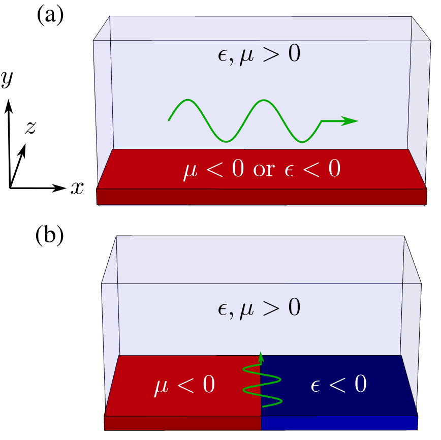
Figure 1: Surface versus line waves: (a) Two dimensional surface waves (plasmons or magnetoplasmons) are bound to the interface between an ordinary dielectric (e.g. air or glass) and a material with either negative permittiviy, $\varepsilon$ or permeability, $\mu$. (b) One dimensional line waves are bound to the interface between three materials; an ordinary dielectric ($y>0$), a negative permittivity material ($y<0,x>0$), and a negative permeability material ($y<0,x<0$).

II The Non–local surface wave equation

Rather than consider the bulk media sketched in Fig.1, where we would have to consider the wave in the region $y<0$, it is simpler to characterize the materials in the half space $y<0$ in terms of a boundary condtion at $y=0$: in terms of a surface impedance. To achieve this on the surface $y=0$, we take the electromagnetic field to satisfy an impedance boundary condition sievenpiperthesis ; senior1995 ,

$$\boldsymbol{E}_{||}=\text{i}\eta_{0}\chi(x)\boldsymbol{\hat{y}\times H}_{||}$$ (1)

where $\chi(x)$ is the surface reactance (surface impedance, $Z=\sqrt{\mu/\varepsilon}=\text{i}\chi$). Our first aim is to re–write this equation as an effective wave equation, written entirely in terms of the behaviour of the in–plane $\boldsymbol{H}$ field on the $y=0$ surface. To eliminate the in–plane electric field field from (1) we apply the Maxwell equation, $\boldsymbol{\nabla\times}\eta_{0}\boldsymbol{H}=-{\rm i}k_{0}\boldsymbol{E}$,

$$\boldsymbol{E}_{||}=\frac{\text{i}\eta_{0}}{k_{0}}\boldsymbol{\hat{y}\times}\left(\frac{\partial\boldsymbol{H}_{||}}{\partial y}-\boldsymbol{\nabla}_{||}H_{y}\boldsymbol{}\right)$$ (2)

where $k_{0}=\omega/c$ and $\eta_{0}=\sqrt{\mu_{0}/\varepsilon_{0}}$.

Although Eqns. (1–2) can be combined into a single equation that describes the components of the magnetic field on the surface alone, it is not yet the ‘surface wave equation’ we want: the equation does not make reference to the behaviour of the field in the plane of the surface alone. We therefore cannot yet find a solution using data on the surface alone until we have removed the third dimension entirely, eliminating both the unknown derivatives normal to the plane, and the normal field component $H_{y}$.

The out of plane field components and derivatives can be eliminated from Eq. (2) through using a Fourier decomposition of the magnetic field, in terms of Fourier amplitudes $\tilde{\boldsymbol{H}}_{||}$. For instance, $\partial\boldsymbol{H}_{||}/\partial y$ can be written as an in–plane convolution of $\boldsymbol{H}_{||}$ with a kernel $K(x-x^{\prime}),$

$$\left.\frac{\partial\boldsymbol{H}_{||}}{\partial y}\right|_{y=0} =-\text{e}^{\text{i}k_{z}z}\int_{-\infty}^{\infty}\frac{\text{d}k}{2\pi}\sqrt{k^{2}+\kappa^{2}}\boldsymbol{\tilde{H}}_{||}(k)\text{e}^{\text{i}kx}$$

$$=\int_{-\infty}^{\infty}\text{d}x^{\prime}K(x-x^{\prime})\left({\boldsymbol{\nabla}_{||}^{\prime}}^{2}+k_{0}^{2}\right)\boldsymbol{H}_{||}(x^{\prime},z)$$ (3)

where $\kappa=(k_{z}^{2}-k_{0}^{2})^{1/2}$. The integration kernel in Eq. (3) is proportional to a modified Bessel function of zeroth order NIST:DLMF

$$K(x-x^{\prime}) =\int_{-\infty}^{\infty}\frac{\text{d}\xi}{2\pi}\frac{\text{e}^{\text{i}\xi\kappa(x-x^{\prime})}}{\sqrt{\xi^{2}+1}}$$

$$=\frac{1}{\pi}K_{0}(\kappa|x-x^{\prime}|).$$ (4)

In the above we assume $k_{z}>k_{0}$ so that—via momentum conservation—the surface wave remains confined, whatever the inhomogeneity of the surface impedance in $x$. This assumption leads to the real valued modified Bessel function in (4). For $k_{z}<k_{0}$, the kernel becomes complex valued, ultimately making our problem non–Hermitian due to the scattering of the wave into the space above the surface.

The basic idea of this section is encapsulated in Eq. (3): we can reformulate the boundary condition (1) entirely in terms of the behaviour of the magnetic field on the surface alone. The price is that the resulting equation is non–local, involving an exponentially localized kernel $K(x-x^{\prime})$ that in Eq. (3) averages the Helmholtz equation over the surface (for the form of the kernel see Fig. 2) . The same calculation can also be performed to eliminate the out of plane magnetic field $H_{y}$ from (2), using the condition $\boldsymbol{\nabla\cdot H}=0$

$$H_{y}=\int\text{d}x^{\prime}\boldsymbol{\nabla}_{||}^{\prime}\cdot\boldsymbol{H}_{||}(x^{\prime})K(x-x^{\prime})$$ (5)

Substituting Eqns. (3) and (5) into (1) and (2) then gives us the final non–local equation governing the field on the surface

$$\int_{-\infty}^{\infty}\text{d}x^{\prime}K(x-x^{\prime})(\boldsymbol{\nabla}_{||}^{\prime}\times\boldsymbol{\nabla}_{||}^{\prime}\times-k_{0}^{2})\boldsymbol{H}_{||}(x^{\prime})+k_{0}\chi(x)\boldsymbol{H}_{||}=0$$ (6)

This is the equation that governs the field on an impedance boundary, making no reference to the space above the surface. To some, Eq. (6) might be a pleasing result: it is a generalization of the two dimensional vector Helmholtz equation $\boldsymbol{\nabla}_{||}\times\boldsymbol{\nabla}_{||}\times\boldsymbol{H}_{||}-k_{0}^{2}\mu\boldsymbol{H}_{||}=0$, the free space equation appearing within the integrand of (6), and the surface reactance playing a role similar to a magnetic susceptibility. The fact that there is a third dimension normal to the surface is encoded in the integral kernel $K(x-x^{\prime})$ defined in Eq. (4), which acts to ‘blur’ the wave operator $\boldsymbol{\nabla}_{||}\times\boldsymbol{\nabla}_{||}\times-k_{0}^{2}$ on the surface. As shown in Fig. 2, as the propagation constant $k_{z}$ is increased, this blurring reduces, reflecting the increasing confinement of the field to the surface.

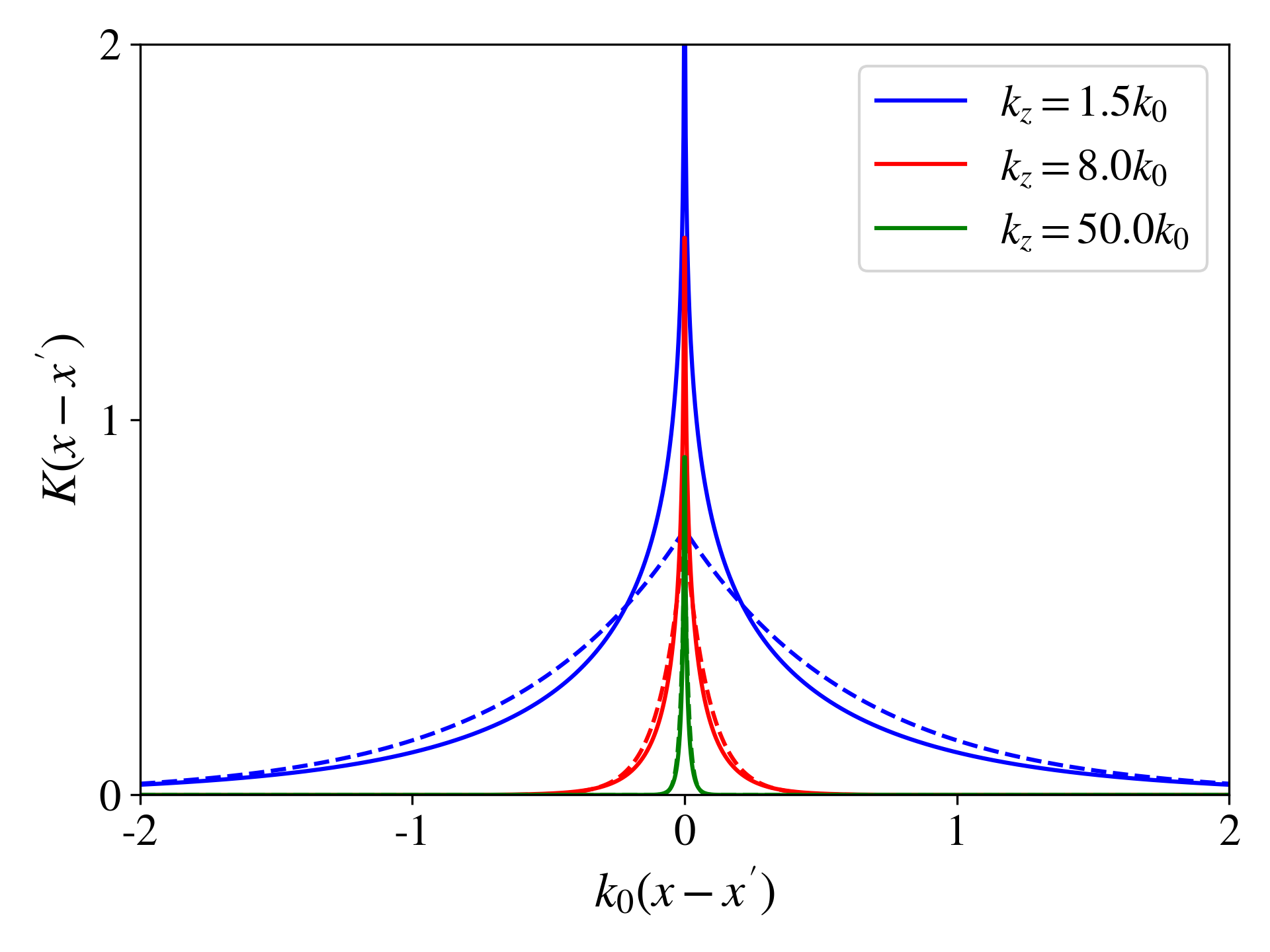
Figure 2: Kernel in the non–local Helmholtz equation (6): Defined in Eq. (4), the integral kernel appearing in the surface Helmholtz equation (6) becomes increasingly localized as the propagation constant $k_{z}/k_{0}$ is increased. Dashed lines show the approximation $K^{(1)}$ given in (16), which becomes increasingly accurate as $k_{z}/k_{0}$ is increased.

II.1 Example: propagation on a homogeneous surface

Before applying our integral equation (6) to line waves, the reader might need convincing that this equation reproduces known results. For a surface with a uniform impedance it is simple to solve Eq. (6). Given it’s Fourier representation (4), the integral kernel $K(x-x^{\prime})$ has plane wave eigenfunctions,

$$\int_{-\infty}^{\infty}\text{d}x^{\prime}K(x-x^{\prime})\text{e}^{\text{i}kx^{\prime}}=\frac{\text{e}^{\text{i}kx}}{\sqrt{k^{2}+\kappa^{2}}}$$ (7)

Therefore, writing the in–plane magnetic field as a plane wave times a constant vector amplitude, $\boldsymbol{H}_{||}(x)=\boldsymbol{H}_{0}\,\text{e}^{\text{i}kx}$, the integral equation (6) becomes a simple algebraic equation that is identical to the dispersion relation for electromagnetic waves in a magnetic material in two dimensions

$$\left[\boldsymbol{k}\times\boldsymbol{k}\times+k_{0}^{2}\;\mu_{\operatorname{eff}}(\boldsymbol{k})\right]\boldsymbol{H}_{0}=0$$ (8)

where $\boldsymbol{k}=k\boldsymbol{\hat{x}}+k_{z}\boldsymbol{\hat{z}}$. The effective permeability in Eq. (8) is given by

$$\mu_{\operatorname{eff}}(\boldsymbol{k})=1-\frac{\sqrt{k^{2}+\kappa^{2}}}{k_{0}}\chi.$$ (9)

Interestingly, unlike the ordinary dispersion relation for electromagnetic waves in two dimensions, the effective permeability for our surface waves (9) depends on the in–plane wave–vector $\boldsymbol{k}$. Surface waves bound to a uniform impedance boundary are thus equivalent to two–dimensional electromagnetic waves in a spatially dispersive magnetic material. There is a very good physical reason for this: if the effective permittivity (9) was not spatially dispersive, there would only be a single transverse magnetic (TM) surface mode with dispersion relation $k^{2}+k_{z}^{2}=\mu_{\operatorname{eff}}k_{0}^{2}$ (there is only one transverse polarization in two dimensions). The fact that the effective permeability (9) is $\boldsymbol{k}$ dependent means that there are both longitudinal (TE) and transverse (TM) wave solutions to the two dimensional equation (8).

The longitudinal (TE) surface mode can be derived through performing an inner product of (8) with $\boldsymbol{k}$, which reduces the dispersion relation to the condition $\mu_{\operatorname{eff}}(\boldsymbol{k})=0$, familiar from the theory of longitudinal modes in spatially dispersive crystals hopfield1963 ,

$$\;\mu_{\operatorname{eff}}(\boldsymbol{k})(\boldsymbol{k}_{||}\cdot\boldsymbol{H}_{0})=\left[k_{0}-\sqrt{k^{2}+\kappa^{2}}\chi\right](\boldsymbol{k}_{||}\cdot\boldsymbol{H}_{0})=0$$ (10)

i.e. $(k^{2}+\kappa^{2})^{1/2}=k_{0}/\chi$. This condition can only be fulfilled when the surface reactance is positive. Meanwhile, taking $\boldsymbol{k\cdot H}_{||}=0$ in (8) yields the dispersion relation for transverse (TM) surface modes,

$$\left[(k^{2}+\kappa^{2})+k_{0}\sqrt{k^{2}+\kappa^{2}}\chi\right]\boldsymbol{H}_{0}=0$$ (11)

i.e. $(k^{2}+\kappa^{2})^{1/2}=-k_{0}\chi$, which can only be fulfilled when the surface reactance is negative. Equations (10) and (11) are the well–known dispersion relations for transverse electric (TE) and transverse magnetic (TM) surface waves sievenpiperthesis ; tretyakov2003 , here derived as a special case of the non–local surface Helmholtz equation (6).

III Line Waves on isotropic surfaces

We now apply the non–local surface wave equation (6) to the central problem of this paper: electromagnetic line waves confined to the $x=0$ interface between two impedance boundaries. To set up this problem we write the surface reactance distribution representing the materials sketched in Fig. 1b in terms of the average reactance $\chi_{b}$, and the contrast $\Delta\chi$,

$$\chi(x)=\chi_{b}+\frac{\Delta\chi}{2}\operatorname{sign}(x).$$ (12)

With this identification, the surface integral equation (6) becomes an eigenvalue problem for the average reactance $\chi_{b}$

$$-\frac{1}{k_{0}}\int_{-\infty}^{\infty}\text{d}x^{\prime}K(x-x^{\prime})(\boldsymbol{\nabla}_{||}^{\prime}\times\boldsymbol{\nabla}_{||}^{\prime}\times-k_{0}^{2})\boldsymbol{H}_{||}(x^{\prime})-\frac{1}{2}\Delta\chi\operatorname{sign}(x)\boldsymbol{H}_{||}=\chi_{b}^{(0)}\boldsymbol{H}_{||}.$$ (13)

The superscript ‘$(0)$’ has been added to the average reactance to indicate that this is the eigenvalue of the equation without approximations. We thus determine the line mode dispersion relation through specifying the wave–number $k_{0}$, the $k_{z}$ wave–vector component, and the reactance contrast $\Delta\chi$. The eigenvalue of the integral equation (13) then gives the average surface reactance required such that the given mode $\boldsymbol{H}_{||}$ is supported for these values of $k_{0}$, $k_{z}$, and $\Delta\chi$.

Numerically it is simplest to solve (13) in the Fourier domain where using the eigenfunctions of the kernel (7) the integral operator becomes a simple multiplication, and the term proportional to $\Delta\chi$ becomes a principal value integral

$$\frac{1}{k_{0}}\left(\boldsymbol{}\frac{\boldsymbol{k}\times\boldsymbol{k}\times+k_{0}^{2}}{\sqrt{k^{2}+\kappa^{2}}}\right)\cdot\tilde{\boldsymbol{H}}_{||}(k)+\frac{\text{i}\Delta\chi}{2}\frac{1}{\pi}\text{P}\int_{-\infty}^{\infty}\frac{\tilde{\boldsymbol{H}}_{||}(k^{\prime})}{k-k^{\prime}}\text{d}k^{\prime}=\chi_{b}^{(0)}\tilde{\boldsymbol{H}}_{||}(k),$$ (14)

where $\tilde{\boldsymbol{H}}_{||}$ is the Fourier transform of the in–plane magnetic field, and ‘P’ indicates the principal part of the integral, which itself is a Hilbert transform king2009 . The appearance of a Hilbert transform is expected in this problem: it’s eigenfunctions are the functions of $k$ that are analytic in either the upper or lower half of the complex $k$ plane, which represent real space functions that are confined to either side of the $x=0$ line, where the reactance takes a fixed value.

Equation (14) can be solved using the Wiener–Hopf method kisil2021 , although we don’t pursue this here. It is also straightforward to solve this equation numerically. To do this we discretize both the $x$–axis and $k$–space into $N$ points and write the left hand side of Eq. (14) as a $2N\times 2N$ matrix with the Hilbert transform written as $\hat{\mathcal{H}}=-\text{i}\hat{\mathcal{F}}^{-1}\operatorname{diag}(\operatorname{sign}(x_{n}))\hat{\mathcal{F}}$ implemented in terms of the discrete Fourier transform matrix $\hat{\mathcal{F}}_{nm}=\exp\left(-\text{i}k_{n}x_{m}\right)$. When written in this matrix form it is evident that, for real $\Delta\chi$ the left hand side of (14) is a Hermitian operator with corresponding real eigenvalues, $\chi_{b}^{(0)}$. For purely imaginary $\Delta\chi$ the system is PT–symmetric, and the operator on the left of (14) is equivalent to a real–valued but non–Hermitian matrix with eigenvalues that are thus real, or in complex conjugate pairs. This is consistent with the findings of moccia2020 , where it was found that line waves can be supported on impedance surfaces with balanced loss and gain.

As the eigenvectors of the operator (14) include both propagating modes and line waves, numerically we sort them by the proportion of their norm concentrated in a small region around $x=0$, neglecting all but the most confined modes. Fig. 3a–b shows the line wave dispersion relation and field profiles calculated using this method, which—as shown—agrees with the same calculation carried out using commercial finite element software (COMSOL multiphysics comsol ).

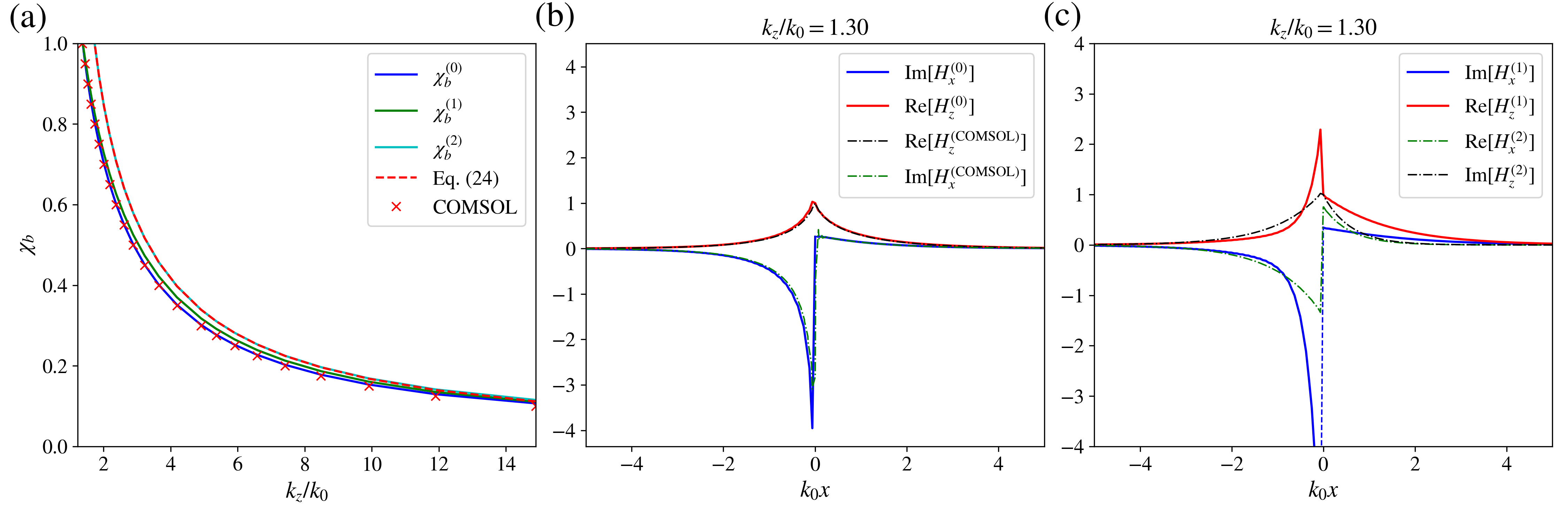
Figure 3: Line mode dispersion and field profiles: (a) Dispersion relation ($\chi_{b}$ as a function of $k_{z}$, for a fixed reactance contrast $\Delta\chi=2.309$) numerically calculated using exact integral equation (14), the two approximations given in (16) and (17), and analytic relation (24). The $800\times 800$ discrete Fourier transform matrix was constructed using spatial periodicity $L=8\lambda$.  Red crosses show calculated values of $k_{z}/k_{0}$ computed using the COMSOL Multiphysics eigenvalue solver. Note that the results of Eqns. (17) (cyan) and (24) (red dashed) are identical. (b) Comparison of in–plane magnetic field profiles $\boldsymbol{H}_{||}$ calculated from the exact integral equation (14) and from COMSOL Multiphysics. (c) Field profiles calculated using approximations (16) and (17).

III.1 Approximations to the integral kernel

The numerical results shown in Fig. 3 show that the line wave has some superficial similarities with an electromagnetic surface wave. For the surface plasmon/magnon, the asymptotic limit, $k_{z}/k_{0}\rightarrow\infty$ requires two bulk media with zero average permittivity/permeability. Equivalently Fig. 3a shows that for line waves, the average surface reactance tends to zero in the same limit. This similarity was also discussed in the asymptotic analysis of Ref. horsley2014 . Moreover the field profiles shown in Fig. 3b suggest that we might make an exponential approximation to the form of the line wave, equivalent to the exponential localization of a surface plasmon/magnon around the interface. In this section we show that we can develop local approximations to the integral kernel $K(x-x^{\prime})$. The leading order approximation then yields a line mode that is the exact two dimensional equivalent of the surface plasmon/magnon, with a dispersion relation that closely matches the numerical solution to Eq. (14).

For inhomogeneous media the difficulty in developing an algebraically simple solution to the non–local equation (13) can be traced back to the square root denominator in the Fourier representation of the integral kernel (4). Were the square root denominator replaced with a polynomial $a_{n}k^{n}+a_{n-1}k^{n-1}+\cdots$, the inverse of the integral operator would be a differential operator $a_{n}\left(-\text{i}\partial_{x}\right)^{n}+a_{n-1}\left(-\text{i}\partial_{x}\right)^{n-1}+\ldots$, meaning that we could re–write (13) as a differential equation. However, the branch cuts in the square root denominator make this simplification impossible. To make progress we recognise that the Fourier transform of an exponentially localized field (such as the line waves we are seeking to describe) is centred around zero wave–vector. We therefore replace the square root denominator in the Fourier representation of the kernel (4) with its series expansion. Here we consider two such approximations,

$$\sqrt{\xi^{2}+1}\sim\left\{\begin{array}[]{lc}1+\frac{1}{2}\xi^{2}&(\operatorname{Approx}.1)\\ &\\ 1&(\operatorname{Approx}.2).\end{array}\right.$$ (15)

These approximations transform the integrand in (4), which contains two square root branch cuts at $\xi=\pm\text{i}$ into a form that is either an entire function of $k$, or contains simple poles. The corresponding approximate expressions for the integral kernel (4) are then given by

$$K^{(1)}(x-x^{\prime})=\int_{-\infty}^{\infty}\frac{\text{d}\xi}{2\pi}\frac{\text{e}^{\text{i}\xi\kappa(x-x^{\prime})}}{\left(1+\frac{1}{2}\xi^{2}\right)}=\frac{\text{e}^{-\sqrt{2}\kappa|x-x^{\prime}|}}{\sqrt{2}}\qquad(\operatorname{Approx}.1)$$ (16)

and

$$K^{(2)}(x-x^{\prime})=\int_{-\infty}^{\infty}\frac{\text{d}\xi}{2\pi}\text{e}^{\text{i}\xi\kappa(x-x^{\prime})}=\frac{1}{\kappa}\delta(x-x^{\prime})\qquad(\operatorname{Approx}.2)$$ (17)

As shown in Fig. 2, the first approximation $K^{(1)}$ closely matches the exact expression (4), becoming ever more accurate as the value of $k_{z}/k_{0}$ is increased. The second approximation (17) only corresponds to the exact kernel in that it matches the area underneath its curve. The dispersion relations and field profiles obtained using these two approximations are compared to the results of the exact equation (14) in Figs. 3 and 4, illustrating that both approximations provide a good estimate of the dispersion of line waves. As shown there, approximation 1 yields fields that have a similar dependence to the exact solution away from the interface, but all field components are discontinuous across $x=0$. Meanwhile approximation 2 tends to underestimate the localization of the field.

III.2 Local line wave equations

The advantage of the approximations (16–17) is that—as discussed above—they reduce the non–local equation (13) to an ordinary differential equation on the surface: an equation written entirely in terms of the surface fields and their in–plane derivatives. For the first approximation (16) we note that $K^{(1)}$ obeys the inhomogeneous equation $(\partial_{x}^{2}-2\kappa^{2})K^{{}^{(1)}}=-2\kappa\delta(x-x^{\prime})$. Therefore, applying the differential operator $\partial_{x}^{2}-2\kappa^{2}$ to Eq. (13) yields a local surface wave equation holding on the $y=0$ surface

$$(\boldsymbol{\nabla}_{||}\times\boldsymbol{\nabla}_{||}\times-k_{0}^{2})\boldsymbol{H}_{||}(x)-\frac{k_{0}}{2\kappa}\left(\frac{\text{d}^{2}}{\text{d}x^{2}}-2\kappa^{2}\right)\chi(x)\boldsymbol{H}_{||}=0\qquad(\operatorname{Approx}.1)$$ (18)

Similarly, using the more extreme approximation (17) where the integral kernel is proportional to a delta function, Eq. (13) becomes

$$\left[\boldsymbol{\nabla}_{||}\times\boldsymbol{\nabla}_{||}\times-k_{0}^{2}\left(1-\frac{\kappa}{k_{0}}\chi(x)\right)\right]\cdot\boldsymbol{H}_{||}(x)=0.\qquad(\operatorname{Approx}.2)$$ (19)

Note that this equation is equivalent to our earlier one for propagation on a homogeneous surface (8) but with $k=0$, and the reactance promoted to a position dependent quantity. It is also worth noticing that taking the $k_{z}/k_{0}\rightarrow\infty$ limit of the first approximate equation (18) yields the second approximation (19).

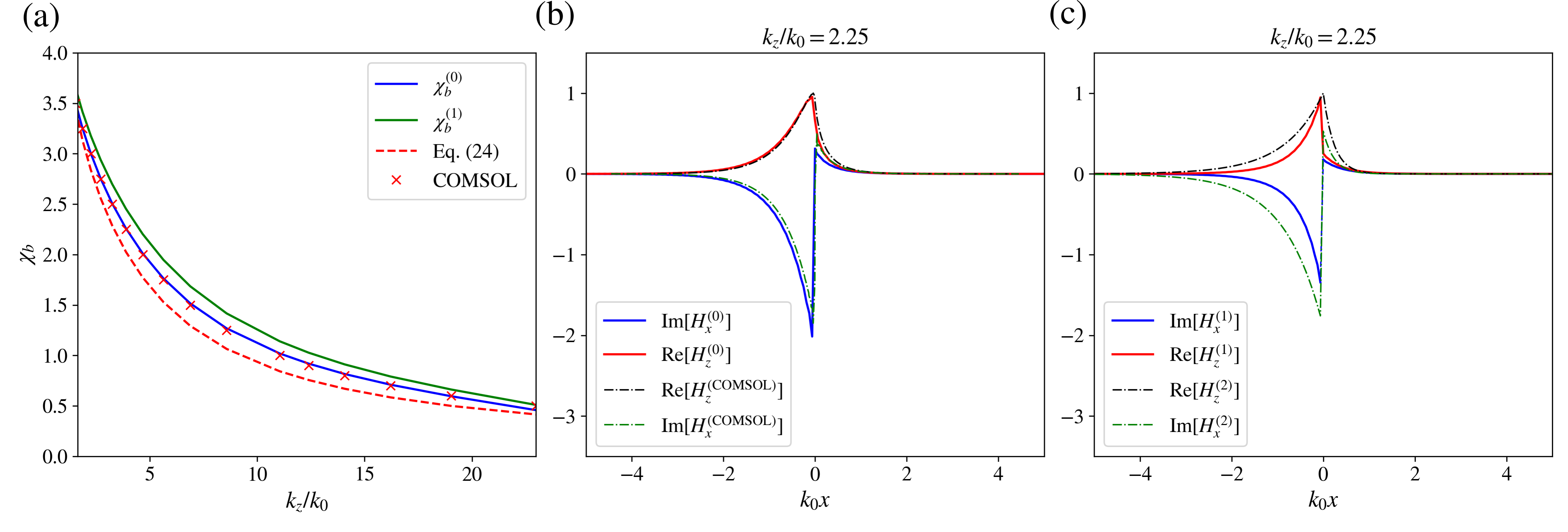
Figure 4: Description as in Fig. 3, but for the increased reactance contrast $\Delta\chi=8.309$, illustrating that the approximate kernels (16–17) give reduced accuracy for larger contrast reactance surfaces.

III.3 Fields and dispersion relations

From the above two surface wave equations (18–19) we can find analytic expressions for the field profiles and dispersion relations of line waves that closely match the results of finite element simulations. In this approximation the field exponentially decays away from $x=0$, and line waves are the direct one–dimensional analogues of surface waves.

We concentrate on the simplest case, Eq. (19), although exactly the same argument can be carried out for the more accurate equation (18) (see Appendix B). Taking the $x$ component of Eq. (19) we find that the $x$ component of the magnetic field is determined by the derivative of $H_{z}$

$$H_{x}=-\frac{\text{i}k_{z}}{\kappa^{2}+k_{0}\kappa\chi(x)}\frac{\text{d}H_{z}}{\text{d}x}.$$ (20)

This expression for $H_{x}$ allows us to write the approximate surface wave equation (19) in terms of $H_{z}$ alone

$$\frac{\text{d}}{\text{d}x}\left(\frac{k_{0}^{2}-k_{0}\kappa\chi(x)}{\kappa^{2}+k_{0}\kappa\chi(x)}\right)\frac{\text{d}H_{z}}{\text{d}x}-k_{0}^{2}\left(1-\frac{\kappa}{k_{0}}\chi(x)\right)H_{z}=0.$$ (21)

Although we are describing the electromagnetic field on a surface, Eq. (21), which governs the cross–sectional form of the line wave, is equivalent to the familiar Helmholtz equation for propagation along a single axis in a bulk electromagnetic material where the effective permittivity is given by

$$\varepsilon_{\operatorname{eff}}=-\frac{\left(\frac{\kappa}{k_{0}}\right)^{2}+\frac{\kappa}{k_{0}}\chi(x)}{1-\frac{\kappa}{k_{0}}\chi(x)}$$ (22)

and the effective permeability, $\mu_{\operatorname{eff}}$ equals (9). By analogy with bulk electromagnetic waves, we can predict the presence of line waves. These waves require provided the product $\varepsilon_{\operatorname{eff}}\mu_{\operatorname{eff}}$ is negative on both sides of the interface (for exponential decay, rather than propagation), in addition to $\varepsilon_{\operatorname{eff}}$ changing sign across the interface (ensuring the decay constant changes sign across $x=0$).

Although the above derivation holds for any spatially varying reactance $\chi(x)$, we consider the special case of the step change in impedance given by (12). From a cursory inspection of Eq. (21) we see that in order that $H_{z}$ is a well defined solution, both $H_{z}$ and $\varepsilon_{\operatorname{eff}}^{-1}\partial_{x}H_{z}$ must be continuous across the impedance interface at $x=0$. Given that the impedance is homogeneous everywhere except at $x=0$, we can thus write the solution to Eq. (21) as a piece–wise function

$$H_{z}=H_{0}\begin{cases}\text{e}^{\beta_{L}x}&\qquad(x<0)\\ &\\ \text{e}^{-\beta_{R}x}&\qquad(x>0)\end{cases}$$ (23)

where, from substitution into (21) we determine the decay constants to be given by  $\beta_{L,R}=\sqrt{\kappa^{2}+k_{0}\kappa\chi^{(L,R)}}$. In this approximation the existence of the line wave thus requires the positivity of $\kappa^{2}+k_{0}\kappa\chi^{(L,R)}$ on either side of the $x=0$ interface. Applying the second condition, for continuity of $\varepsilon_{\operatorname{eff}}^{-1}\partial_{x}H_{z}$ then yields the line–wave dispersion relation

$$\left(1-\frac{\kappa}{k_{0}}\chi^{(L)}\right)\sqrt{\frac{\kappa}{k_{0}}+\chi^{(R)}}+\left(1-\frac{\kappa}{k_{0}}\chi^{(R)}\right)\sqrt{\frac{\kappa}{k_{0}}+\chi^{(L)}}=0$$ (24)

which—as shown in Figs. 3 and 4—provides a good estimate of the numerically determined dispersion relation calculated from the exact Eq. (14), and using finite element simulations. From (24) we can see that, as $k_{z}\rightarrow\infty$, the dispersion relation reduces to

$$k_{z}\rightarrow\infty:\qquad\chi^{(L)}+\chi^{(R)}=0$$ (25)

in agreement with the asymptotic analysis given in horsley2014 . For complex reactances, this condition implies a PT–symmetric surface with balanced loss and gain, as found in moccia2020 . We can therefore see that, despite the apparently complicated mathematical properties of line waves, they can be reasonably approximated as exponentially decaying fields on the surface, obeying the two–dimensional equation (19) which could have been anticipated from boldly promoting the dispersion relation on a homogeneous surface to a wave equation (8).

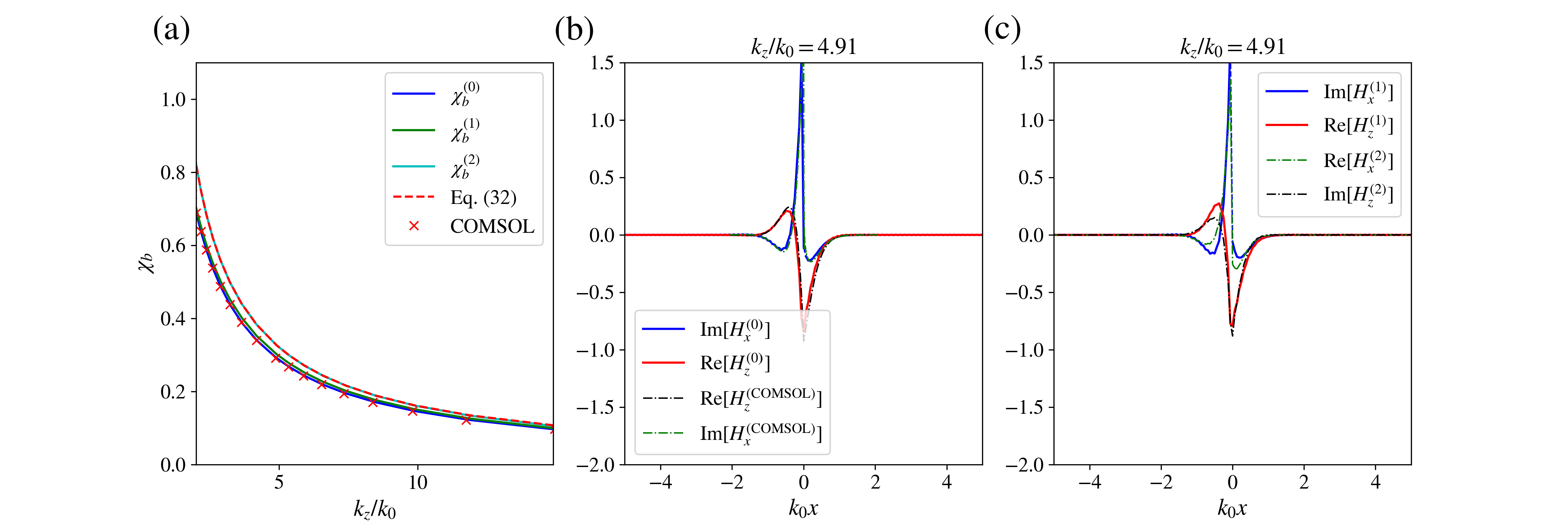
Figure 5: Line wave profiles on an anisotropic surface with $\Delta\boldsymbol{\chi}=\left(\begin{array}[]{cc}2.5&1.2\\ 1.2&2.5\end{array}\right)$ and $\boldsymbol{\chi}_{a}=0$, as defined in (27). (a) Dispersion relations obtained using the exact integral equation (27), the two approximations (16) and (17), the analytic dispersion relation (33), and finite element simulations (see Appendix A).  Panels (b) and (c) show that the mode oscillates as it decays, characteristic of ‘ghost’ line waves moccia2023 , an effect that is still captured by the most extreme approximation to the integral kernel (29) .

IV Anisotropic surfaces: Effective Gauge fields, and ghost waves

Finally, having derived this simple theory for isotropic impedance boundaries we can explore some extensions to more exotic surfaces. The most obvious generalization is to anisotropic impedance boundaries. These were very recently been discussed in Ref. moccia2023 , where primarily using finite element simulations, one–dimensional “ghost line waves” were discovered: confined waves on a lossless surface that oscillate as they decay. Here we shall show that this hybrid behaviour can be straightforwardly explained using the local approximation to our integral equation described above. Put simply, the anisotropy acts as an effective gauge field on the surface, and just as for an electron subject to a magnetic vector potential peshkin2014 , this induces extra oscillations in the surface field.

To treat anisotropic impedance boundaries, we assume the anisotropic generalization of the surface reactance profile given in Eq. (12)

$$\boldsymbol{\chi}(x)=\chi_{b}\boldsymbol{1}_{2}+\boldsymbol{\chi}_{a}+\frac{\Delta\boldsymbol{\chi}}{2}\operatorname{sign}(x)$$ (26)

where $\Delta\boldsymbol{\chi}$ is the tensorial difference in the reactance between the two surfaces, a Hermitian matrix in the case of lossless surfaces. 6 The matrix $\boldsymbol{\chi}_{a}$ is a constant matrix representing the zero–trace part of the average reactance of the two surfaces, whereas $\chi_{b}$ is an overall shift to the diagonal elements of the surface reactance required to support the surface wave. With this reactance profile the integral equation (14) is simply generalized to,

$$\left(\frac{1}{k_{0}}\boldsymbol{}\frac{\boldsymbol{k}\times\boldsymbol{k}\times+k_{0}^{2}}{\sqrt{k^{2}+\kappa^{2}}}-\boldsymbol{\chi}_{a}\right)\cdot\widetilde{\boldsymbol{H}}_{||}(k)+\frac{\Delta\boldsymbol{\chi}\cdot}{2}\frac{\text{i}}{\pi}\text{P}\int_{-\infty}^{\infty}\frac{\widetilde{\boldsymbol{H}}_{||}(k^{\prime})}{k-k^{\prime}}\text{d}k^{\prime}\cdot\widetilde{\boldsymbol{H}}_{||}(k)=\chi_{b}^{(0)}\widetilde{\boldsymbol{H}}_{||}(k).$$ (27)

This remains a Hermitian operator for Hermitian $\Delta\boldsymbol{\chi}$ and $\boldsymbol{\chi}_{a}$, indicating eigenmodes are still supported for real values of the diagonal reactance components, $\chi_{b}^{(0)}$.

By an identical argument to that presented in Sec. III.2, the more extreme of the two local approximations to this integral equation is also a straightforward generalization of our surface vector Helmholtz equation (19), where the reactance is replaced with a $2\times 2$ matrix,

$$(\boldsymbol{\nabla}_{||}\times\boldsymbol{\nabla}_{||}\times-k_{0}^{2})\boldsymbol{H}_{||}(x)+\kappa k_{0}\boldsymbol{\chi}\cdot\boldsymbol{H}_{||}=0$$

$$\rightarrow H_{x}=-\frac{1}{\kappa^{2}+k_{0}\kappa\chi_{xx}}\left(ik_{z}\frac{\text{d}}{\text{d}x}+k_{0}\kappa\chi_{xz}\right)H_{z}.$$ (28)

The second line follows from taking the $x$–component of the Helmholtz equation, which determines the component of the magnetic field orthogonal to the propagation axis. Interestingly, a comparison with our earlier Eq. (20) shows that the off–diagonal element $\chi_{xz}$ induces an effective gauge potential in (28), modifying the derivative to $\partial_{x}-\text{i}k_{z}^{-1}k_{0}\kappa\chi_{xz}$. The appearance of an effective gauge field in the line-wave equation due to the anisotropy is confirmed after substituting Eq. (28) into the preceding vector Helmholtz equation, where we are left with a second order equation for the field component $H_{z}$

$$\left(\frac{d}{dx}-\text{i}A\right)\frac{1}{\varepsilon_{\operatorname{eff}}}\left(\frac{d}{dx}-\text{i}A\right)H_{z}+k_{0}^{2}\mu_{\operatorname{eff}}H_{z}=0.$$ (29)

Here we have assumed a symmetric reactance $\chi_{xz}=\chi_{zx}$ which is equivalent to assuming time reversal symmetry of the surface (for a Hermitian reactance, both $A$ and its complex conjugate appear in  (29)). In this case the effective gauge potential is given by $A=\sigma k_{z}\kappa k_{0}^{-1}\chi_{xz}$, where $\sigma=[1-(\kappa/k_{0})\chi_{xx}]^{-1}$. Meanwhile the effective permittivity and permeability are generalized from the earlier expressions (9) and (22) to $\varepsilon_{\operatorname{eff}}=-\sigma[(\kappa/k_{0})^{2}+(\kappa/k_{0})\chi_{xx}]$, and $\mu_{\operatorname{eff}}=\sigma[1-(\kappa/k_{0})\operatorname{Tr}(\boldsymbol{\chi})+(\kappa/k_{0})^{2}\det(\boldsymbol{\chi})]$.

The Helmholtz equation (29) takes the form of the one dimensional Schrödinger equation for a charged particle in a magnetic gauge potential $A$ with a mass proportional to $\varepsilon_{\operatorname{eff}}$ and a scalar potential proportional to $\mu_{\operatorname{eff}}$ peshkin2014 . The effect of the anisotropy on the surface field thus both modifies the dispersion relation (24) due to the generalized forms of $\varepsilon_{\operatorname{eff}}$ and $\mu_{\operatorname{eff}}$, as well as introducing field oscillations along the $x$–axis. These oscillations due to the gauge field can be isolated through making the substitution, $H_{z}=\exp\left(\text{i}\int_{0}^{x}A(x^{\prime})\text{d}x^{\prime}\right)h_{z}$. 6 This substitution transforms the field equation (29), to an equation for $h_{z}$ that takes the earlier form (21)

$$\frac{d}{dx}\frac{1}{\varepsilon_{\operatorname{eff}}}\frac{dh_{z}}{dx}+k_{0}^{2}\mu_{\operatorname{eff}}h_{z}=0.$$ (30)

The only difference from our earlier analysis are the modifications to the functional form of the effective permittivity and permeability. Assuming $\varepsilon_{\operatorname{eff}}\mu_{\operatorname{eff}}<0$, Eq. (30) again admits confined line–wave solutions $h_{z}$ of the form (23) with decay constants

$$\beta_{L,R} =k_{0}\sqrt{-\varepsilon_{\operatorname{eff}}\mu_{\operatorname{eff}}}$$ (31)

$$=k_{0}\frac{\sqrt{\left(\frac{\kappa}{k_{0}}\right)^{2}+\frac{\kappa}{k_{0}}\chi_{xx}^{(L,R)}}}{\left|1-\frac{\kappa}{k_{0}}\chi_{xx}^{(L,R)}\right|}\sqrt{1-\frac{\kappa}{k_{0}}\operatorname{Tr}[\boldsymbol{\chi}^{(L,R)}]+\left(\frac{\kappa}{k_{0}}\right)^{2}\det[\boldsymbol{\chi}^{(L,R)}]}$$ (32)

which reduce to those given below Eq. (23) for isotropic surfaces where $\chi_{xx}^{(L,R)}=\chi_{zz}^{(L,R)}$ and $\chi_{xz}^{(L,R)}=\chi_{zx}^{(L,R)}=0$. Again demanding the continuity of $\varepsilon_{\operatorname{eff}}^{-1}\partial_{x}h_{z}$ yields the corresponding line wave dispersion relation

$$\left(1+\frac{k_{0}}{\kappa}\chi_{xx}^{(L)}\right)\left(1-\frac{\kappa}{k_{0}}\chi_{xx}^{(R)}\right)\beta_{L}+\left(1+\frac{k_{0}}{\kappa}\chi_{xx}^{(R)}\right)\left(1-\frac{\kappa}{k_{0}}\chi_{xx}^{(L)}\right)\beta_{R}=0.$$ (33)

This is plotted as the red dashed line in Fig. 5a, where it is evident that for this range of impedance values, this approximation closely matches the results of both the exact integral equation (27) and finite element simulations. Figures 5b and 5c show cross sections of the line wave field, where—compared to the isotropic results shown in Figs. 3–4—there is the anticipated hybrid of oscillation and decay away from the $x=0$ interface on the surface.

As in the isotropic case discussed above and in Ref. horsley2014 , in the asymptotic limit $k_{z}\rightarrow\infty$,the dispersion relation simplifies to a constraint on the material parameters,

$$\frac{\chi_{xx}^{(R)}}{|\chi_{xx}^{(L)}|}\sqrt{\det[\boldsymbol{\chi}^{(L)}]}+\frac{\chi_{xx}^{(L)}}{|\chi_{xx}^{(R)}|}\sqrt{\det[\boldsymbol{\chi}^{(R)}]}=0$$ (34)

which reduces to our previous result (25) when the surface is isotropic. Indeed, for anisotropic surfaces with a reactance matrix of equal determinant $\det[\boldsymbol{\chi}^{(L)}]=\det[\boldsymbol{\chi}^{(R)}]$, Eq. (34) predicts that the asymptotic limit occurs when the diagonal elements $\chi_{xx}^{(L,R)}$ are of equal magnitude and opposite sign.

V Summary and Conclusions

Although wedge plasmons and edge waves are well–known one–dimensional excitations, these are typically confined to a surface through the effect of surface curvature valle2010 . On the other hand, line waves sievenpiper2017 ; horsley2014 ; moccia2020 ; moccia2023 are one–dimensional waves confined to flat surfaces by the distribution of surface impedance. Line waves are much more difficult to theoretically analyse than surface waves, and to–date a simple understanding of these modes has been lacking.

In this work we have provided a new general theory for analysing the behaviour of line waves on impedance boundaries. In the exact case, the properties of line waves can be calculated through determining the eigenfunctions of the integral equation (14), or its generalization to anisotropic surfaces (27). To gain further understanding of these waves, this integral equation can be approximated as a differential equation using the expansions of the kernel (18) and (19), revealing that the cross–section of the line wave obeys a one–dimensional Helmholtz equation on the surface, with a spatially dispersive effective permittivity and permeability. From this we have shown that an approximate line wave dispersion relation can be derived exactly as is done for the surface plasmon/magnon, with the result closely matching the results of finite element simulations (see Fig. 3), deviating more when the impedance contrast is increased to larger values (see Fig. 4).

As we have shown, it is also straightforward to extend this theory to anisotropic impedance boundaries. In this case the cross section of the line wave also (approximately) obeys a one dimensional Helmholtz equation, with the anisotropy modifying the effective permittivity and permeability values, ensuring—for example—that the asymptotic limit of the dispersion relation no longer requires equal and opposite reactance values, but the more complicated combination of material parameters given in Eq. (34). Interestingly, we have also found that anisotropy of the reactance induces an effective gauge field on the surface. As we are dealing with an effective one–dimensional equation, this gauge field cannot induce e.g. cyclotron orbits of the surface wave, but instead is equivalent to the gauge transformation given above Eq. (30) which leads to oscillations in the field away from the interface. We have verified this numerically (see Fig. 5) using both the exact integral equation and finite element simulations, providing an explanation for the recently identified ‘ghost’ line waves moccia2023 .

Just as understanding surfaces waves has led to surface wave antennas and the field of plasmonics, understanding line waves could lead to similar applications. They allow—for instance—electromagnetic energy to be channeled without the use of a waveguide, and as shown above and in moccia2023 the flow of this near–field energy can be moulded via the anisotropy of the surface. The theory presented here may provide a framework for a deeper understanding these waves in a larger parameter space than has been considered to–date.

VI Acknowledgements

SARH and AD thank the Royal Society and TATA for financial support (RPG-2016-186)). SARH thanks Ian Hooper and James Capers for useful discussions.

VII Appendix A: Modifications to comsol

To simulate anisotropic impedance boundaries we modified the equations of the “impedance boundary” in COMSOL Multiphysics. This was done for surfaces with surface normal $\boldsymbol{\hat{y}}$ by replacing the following expressions

emw.imp1.Jsx  = ((Zzz*(emw.tEx+emw.Esx)-Zxz*(emw.tEz+emw.Esz))/dZ)/Z0
emw.imp1.Jsy  = 0
emw.imp1.Jsz  = ((Zxx*(emw.tEz+emw.Esz)-Zzx*(emw.tEx+emw.Esx))/dZ)/Z0

where Z0=377$\Omega$ is the free space impedance, Zxx, Zxz, Zzx, and Zzz are the components of the impedance tensor $\boldsymbol{Z}=i\boldsymbol{\chi}$, and dZ is the determinant of the impedance tensor, all defined as a set of parameters for each impedance boundary in the COMSOL model.

VIII AppenDIX B: the more accurate solution

In the main text we gave analytic results for the very simplest approximation to the integral kernel (4). We can also develop more accurate analytic results for the next order approximation, although the formulae are more complicated. Here we give this more accurate solution for an isotropic impedance boundary. The approximate surface wave equation is given by Eq. (18) in the main text, which we repeat here:

$$(\boldsymbol{\nabla}_{||}\otimes\boldsymbol{\nabla}_{||}-\boldsymbol{\nabla}_{||}^{2}-k_{0}^{2})\boldsymbol{H}_{||}(x)-\frac{k_{0}}{2\kappa}\left(\frac{\text{d}^{2}}{\text{d}x^{2}}-2\kappa^{2}\right)\chi(x)\boldsymbol{H}_{||}=0.$$ (35)

Splitting this equation into components we obtain two coupled Helmholtz equations, one for the $x$–component

$$\frac{k_{0}}{2\kappa}\frac{\text{d}^{2}}{\text{d}x^{2}}(\chi H_{x})-(\kappa^{2}+k_{0}\kappa\chi)H_{x}-\text{i}k_{z}\frac{\text{d}H_{z}}{\text{d}x}=0,$$ (36)

and one for the $z$–component,

$$\frac{\text{d}^{2}}{\text{d}x^{2}}\left(1+\frac{k_{0}}{2\kappa}\chi\right)H_{z}+k_{0}^{2}\left(1-\frac{\kappa}{k_{0}}\chi\right)H_{z}-\text{i}k_{z}\frac{\text{d}H_{x}}{\text{d}x}=0.$$ (37)

Assuming a junction between two surfaces as in (12) we can solve (36–37) by assuming—in the homogeneous regions—that the field has the form

$$\left(\begin{array}[]{c}H_{x}\\ H_{z}\end{array}\right)=\left(\begin{array}[]{c}A_{x}\\ A_{z}\end{array}\right)\text{e}^{\pm\beta x}$$ (38)

($\beta>0$) so that (36–37) can be written as a single matrix equation

$$\left(\begin{array}[]{cc}\frac{k_{0}\chi}{2\kappa}\beta^{2}-(\kappa^{2}+k_{0}\kappa\chi)&\mp\text{i}k_{z}\beta\\ \mp\text{i}k_{z}\beta&\left(1+\frac{k_{0}}{2\kappa}\chi\right)\beta^{2}+k_{0}^{2}\left(1-\frac{\kappa}{k_{0}}\chi\right)\end{array}\right)\left(\begin{array}[]{c}A_{x}\\ A_{z}\end{array}\right)=0,$$ (39)

which requires the matrix to have zero determinant. The zero determinant condition yields a fourth order polynomial in the decay constant $\beta$

$$\left[\frac{k_{0}\chi}{2\kappa}\beta^{2}-(\kappa^{2}+k_{0}\kappa\chi)\right]\left[\left(1+\frac{k_{0}}{2\kappa}\chi\right)\beta^{2}+k_{0}^{2}\left(1-\frac{\kappa}{k_{0}}\chi\right)\right]+k_{z}^{2}\beta^{2}=0.$$ (40)

As Eq. (40) is a quadratic equation in $\beta^{2}$ we have four values of $\beta$ that form two pairs of solutions with the same magnitude

$$\begin{array}[]{cl}\beta_{1}^{2}&=\frac{1}{2a}\left[-b+\sqrt{b^{2}-4ac}\right]\\ &\\ \beta_{2}^{2}&=\frac{1}{2a}\left[-b-\sqrt{b^{2}-4ac}\right].\end{array}$$ (41)

To simplify the notation we have introduced three constants,

$$\begin{array}[]{cl}a&=\frac{k_{0}\chi}{2\kappa}\left(1+\frac{k_{0}}{2\kappa}\chi\right)\\ &\\ b&=\frac{k_{0}\chi}{2\kappa}k_{0}^{2}\left(1-\frac{\kappa}{k_{0}}\chi\right)-(\kappa^{2}+k_{0}\kappa\chi)\left(1+\frac{k_{0}}{2\kappa}\chi\right)+k_{z}^{2}\\ &\\ c&=-(\kappa^{2}+k_{0}\kappa\chi)k_{0}^{2}\left(1-\frac{\kappa}{k_{0}}\chi\right).\end{array}$$ (42)

Therefore, on each side of the interface our field is composed of a combination of two exponentials with decay constants $\beta_{1}$ and $\beta_{2}$ given by Eq. (41). Each of these decaying components is multiplied by the corresponding zero eigenvector of the matrix equation (39) so that on each side of the interface the surface magnetic field takes the form

$$x<0:\qquad\boldsymbol{H}_{||}=c_{1}^{(L)}N_{1}^{(L)}\left(\begin{matrix}\text{i}k_{z}\beta_{1}^{(L)}\\ \\ \frac{k_{0}\chi^{(L)}}{2\kappa}[\beta_{1}^{(L)}]^{2}-(\kappa^{2}+k_{0}\kappa\chi^{(L)})\end{matrix}\right)\text{e}^{\beta_{1}^{(L)}x}\\[10.0pt] +c_{2}^{(L)}N_{2}^{(L)}\left(\begin{matrix}\text{i}k_{z}\beta_{2}^{(L)}\\ \\ \frac{k_{0}\chi^{(L)}}{2\kappa}[\beta_{2}^{(L)}]^{2}-(\kappa^{2}+k_{0}\kappa\chi^{(L)})\end{matrix}\right)\text{e}^{\beta_{2}^{(L)}x}$$ (43)

where $N_{1,2}^{(L,R)}$ are the normalization constants defined as

$$N_{1,2}^{(L,R)}=\frac{1}{\sqrt{\left(\frac{k_{0}\chi^{(L,R)}}{2\kappa}[\beta_{1,2}^{(L,R)}]^{2}-(\kappa^{2}+k_{0}\kappa\chi^{(L,R)})\right)^{2}+k_{z}^{2}[\beta_{1,2}^{(L,R)}]^{2}}}$$ (44)

The constants $c_{1,2}^{(L,R)}$ appearing in Eq. (43) are yet to be determined and their represent the amplitudes of the two different exponentially decaying solutions in the region $x<0$. The field on the right hand side of the $x=0$ line is similarly expressed in terms of two decaying solutions

$$x>0:\qquad\boldsymbol{H}_{||}=c_{1}^{(R)}N_{1}^{(R)}\left(\begin{matrix}-\text{i}k_{z}\beta_{1}^{(R)}\\ \\ \frac{k_{0}\chi^{(R)}}{2\kappa}[\beta_{1}^{(R)}]^{2}-(\kappa^{2}+k_{0}\kappa\chi^{(R)})\end{matrix}\right)\text{e}^{-\beta_{1}^{(R)}x}\\[10.0pt] +c_{2}^{(R)}N_{2}^{(R)}\left(\begin{matrix}-\text{i}k_{z}\beta_{2}^{(R)}\\ \\ \frac{k_{0}\chi^{(R)}}{2\kappa}[\beta_{2}^{(R)}]^{2}-(\kappa^{2}+k_{0}\kappa\chi^{(R)})\end{matrix}\right)\text{e}^{-\beta_{2}^{(R)}x}$$ (45)

To determine the four unknown expansion coefficients in Eqns. (43–45), plus the dispersion relation we must apply four boundary conditions at $x=0$. These four boundary conditions are contained in the two coupled differential equations (36) and (37) derived above. For the solution to hold across the line $x=0$, all differentiated quantities must be continuous. Therefore, from examining the second derivatives in Eqns. (36) and (37) we can see that the first derivatives they contain will only be well defined if $\chi(x)H_{x}$ and $(1+k_{0}\chi/2\kappa)H_{z}$ are continuous. Similarly, integrating these equations across an infinitesimal interval containing $x=0$ we can also see that $\partial_{x}(k_{0}\chi H_{x}/2\kappa)-\text{i}k_{z}H_{z}$ and $\partial_{x}(1+k_{0}\chi/2\kappa)H_{z}-\text{i}k_{z}H_{x}$ are continuous across the interface. These are the four conditions we require to determine the dispersion of the line wave to a more accurate approximation.

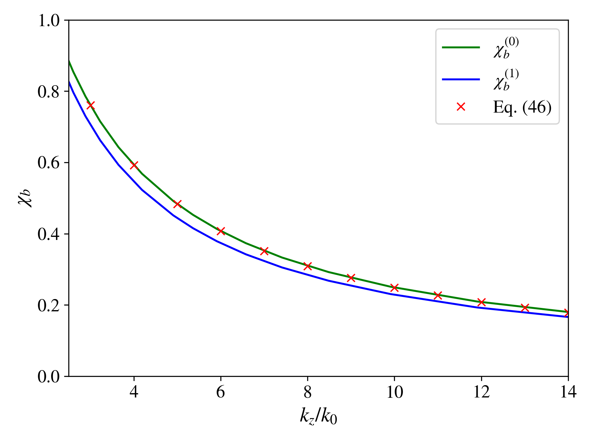
Figure 6: Line wave dispersion for $\Delta\chi=3.209$, with other parameters as in Fig. 3. The analytic expression (47) reproduces the result of using the approximate integral kernel $K^{(1)}$ given in Eq. (16).

Applying these four conditions to the expansions (43) and (45) we find the following $4\times 4$ matrix representation of the boundary conditions,

$$\footnotesize\left(\begin{matrix}N_{1}^{(L)}\beta_{1}^{(L)}\chi^{(L)}&N_{2}^{(L)}\beta_{2}^{(L)}\chi^{(L)}&N_{1}^{(R)}\beta_{1}^{(R)}\chi^{(R)}&N_{2}^{(R)}\beta_{2}^{(R)}\chi^{(R)}\\ N_{1}^{(L)}\Sigma_{1}^{(L)}&N_{2}^{(L)}\Sigma_{2}^{(L)}&-N_{1}^{(R)}\Sigma_{1}^{(R)}&-N_{2}^{(R)}\Sigma_{2}^{(R)}\\ -N_{1}^{(L)}(\kappa^{2}+k_{0}\kappa\chi^{(L)})&-N_{2}^{(L)}(\kappa^{2}+k_{0}\kappa\chi^{(L)})&N_{1}^{(R)}(\kappa^{2}+k_{0}\kappa\chi^{(R)})&N_{2}^{(R)}(\kappa^{2}+k_{0}\kappa\chi^{(R)})\\ N_{1}^{(L)}\beta_{1}^{(L)}(\Sigma_{1}^{(L)}+k_{z}^{2})&N_{2}^{(L)}\beta_{2}^{(L)}(\Sigma_{2}^{(L)}+k_{z}^{2})&N_{1}^{(R)}\beta_{1}^{(R)}(\Sigma_{1}^{(R)}+k_{z}^{2})&N_{2}^{(R)}\beta_{2}^{(R)}(\Sigma_{2}^{(R)}+k_{z}^{2})\end{matrix}\right)\left(\begin{matrix}c_{1}^{(L)}\\ c_{2}^{(L)}\\ c_{1}^{(R)}\\ c_{2}^{(R)}\end{matrix}\right)=0$$ (46)

where $\Sigma_{1,2}^{(L,R)}=\left(1+\frac{k_{0}\chi^{(L,R)}}{2\kappa}\right)\left[\frac{k_{0}\chi^{(L,R)}}{2\kappa}[\beta_{1,2}^{(L,R)}]^{2}-(\kappa^{2}+k_{0}\kappa\chi^{(L,R)})\right]$. The vanishing determinant of this matrix defines the dispersion relation of these modes,

$$\footnotesize\det\left(\begin{matrix}\beta_{1}^{(L)}N_{1}^{(L)}\chi^{(L)}&\beta_{2}^{(L)}N_{2}^{(L)}\chi^{(L)}&\beta_{1}^{(R)}N_{1}^{(R)}\chi^{(R)}&\beta_{2}^{(R)}N_{2}^{(R)}\chi^{(R)}\\ N_{1}^{(L)}\Sigma_{1}^{(L)}&N_{2}^{(L)}\Sigma_{2}^{(L)}&-N_{1}^{(R)}\Sigma_{1}^{(R)}&-N_{2}^{(R)}\Sigma_{2}^{(R)}\\ -N_{1}^{(L)}(\kappa^{2}+k_{0}\kappa\chi^{(L)})&-N_{2}^{(L)}(\kappa^{2}+k_{0}\kappa\chi^{(L)})&N_{1}^{(R)}(\kappa^{2}+k_{0}\kappa\chi^{(R)})&N_{2}^{(R)}(\kappa^{2}+k_{0}\kappa\chi^{(R)})\\ \beta_{1}^{(L)}N_{1}^{(L)}(\Sigma_{1}^{(L)}+k_{z}^{2})&\beta_{2}^{(L)}N_{2}^{(L)}(\Sigma_{2}^{(L)}+k_{z}^{2})&\beta_{1}^{(R)}N_{1}^{(R)}(\Sigma_{1}^{(R)}+k_{z}^{2})&\beta_{2}^{(R)}N_{2}^{(R)}(\Sigma_{2}^{(R)}+k_{z}^{2})\end{matrix}\right)=0,$$ (47)

which is the analytic expression for the more accurate dispersion relation shown in Figs. 3–4. Fig. 6 shows—for an arbitrarily chosen value of $\Delta\chi$—that this expression reproduces the results of the integral equation (13) with the approximate kernel (16).

References

- [1] D. J. Bisharat and D. Sievenpiper. Guiding waves along an infinitesimal line between impedance surfaces. Phys. Rev. Lett., 119:106802, 2017.
- [2] D. J. Bisharat and D. F. Sievenpiper. Electromagnetic-dual metasurfaces for topological states along a 1d interface. Laser & Photonics Reviews, 13:1900126, 2019.
- [3] K. Y. Bliokh, D. Leykam, M. Lein, and F. Nori. Topological non-hermitian origin of surface maxwell waves. Nat. Comm., 10:580, 2019.
- [4] K. Y. Bliokh and F. Nori. Klein-gordon representation of acoustic waves and topological origin of surface acoustic modes. Phys. Rev. Lett., 123:054301, 2019.
- [5] S. Brûlé, E. H. Javelaud, S. Enoch, and S. Guenneau. Experiments on seismic metamaterials: Molding surface waves. Phys. Rev. Lett., 112:133901, 2014.
- [6] G. Della Valle and S. Longhi. Geometric potential for plasmon polaritons on curved surfaces. J. Phys. B, 43:051002, 2010.
- [7] NIST Digital Library of Mathematical Functions. http://dlmf.nist.gov/, Release 1.1.8 of 2022-12-15. F. W. J. Olver, A. B. Olde Daalhuis, D. W. Lozier, B. I. Schneider, R. F. Boisvert, C. W. Clark, B. R. Miller, B. V. Saunders, H. S. Cohl, and M. A. McClain, eds.
- [8] J. J. Hopfield and D. G. Thomas. Theoretical and experimental effects of spatial dispersion on the optical properties of crystals. Physical Review, 132(2):563, 1963.
- [9] S. A. R. Horsley. Indifferent electromagnetic modes: Bound states and topology. Phys. Rev. A, 100:053819, 2019.
- [10] S. A. R. Horsley and I. R. Hooper. One dimensional electromagnetic waves on flat surfaces. J. Phys. D, 47:435103, 2014.
- [11] S. A. R. Horsley and M. Woolley. Zero-refractive-index materials and topological photonics. Nat. Phys., 17:348, 2021.
- [12] COMSOL Inc. Comsol multiphysics, 2022.
- [13] A. B. Khanikaev, S. H. Mousavi, W.-K. Tse, M. Kargarian, A. H. MacDonald, and G. Shvets. Photonic topological insulators. Nat. Mat., 12:233, 2013.
- [14] F.W. King. Hilbert Transforms. Number v. 1 in Encyclopedia of Mathematics an. Cambridge University Press, 2009.
- [15] A. V. Kisil, D. I. Abrahams, G. Mishuris, and S. V. Rogosin. The wiener–hopf technique, its generalizations and applications: constructive and approximate methods. Proceedings of the Royal Society A, 477(2254):20210533, 2021.
- [16] X. Kong, J. B. Dia’aaldin, G. Xiao, and D. F. Sievenpiper. Analytic theory of an edge mode between impedance surfaces. Physical Review A, 99(3):033842, 2019.
- [17] L. D. Landau and E. M. Lifshitz. Theory of Elasticity. Pergamon Press, 1959.
- [18] A. Li, S. Singh, and D. F. Sievenpiper. Metasurfaces and their applications. Nanophotonics, 7:989, 2018.
- [19] E. Martini, M. Mencagli Jr, and S. Maci. Metasurface transformation surface wave control. Phil. Trans. R. Soc. A, 373:20140355, 2015.
- [20] M. Moccia, G. Castaldi, A. Alú, and V. Galdi. Line waves in non-hermitian metasurfaces. ACS Photonics, 7(8):2064–2072, 2020.
- [21] M. Moccia, G. Castaldi, A. Alù, and V. Galdi. Ghost line waves. arXiv:2305.15789, 2023.
- [22] M. Peshkin and A. Tonomura. The Aharonov-Bohm Effect. Springer Berlin-Heidelberg, 2014.
- [23] J. A. Polo, T. G. Mackay, and A. Lakhtakia. Electromagnetic Surface Waves, A Modern Perspective. Elsevier, 2013.
- [24] T. B. A. Senior and J. L. Volakis. Approximate Boundary Conditions in Electromagnetics. Institution of Electrical Engineers, 1995.
- [25] D. F. Sievenpiper. High-impedance electromagnetic surfaces. University of California, Los Angeles, 1999.
- [26] S. Tretyakov. Analytical Modelling in Applied Electromagnetics. Artech House, 2003.
- [27] X. Xu, J. Chang, J. Tong, D. F. Sievenpiper, and T. J. Cui. Near-field chiral excitation of universal spin-momentum locking transport of edge waves in microwave metamaterials. Advanced Photonics, 4:046004, 2022.