Temporal witnesses of non-classicality in a macroscopic biological system

Abstract

Exciton transfer along a polymer is essential for many biological processes, for instance light harvesting in photosynthetic biosystems. Here we apply a new witness of non-classicality to this phenomenon, to conclude that, if an exciton can mediate the coherent quantum evolution of a photon, then the exciton is non-classical. We then propose a general qubit model for the quantum transfer of an exciton along a polymer chain, also discussing the effects of environmental decoherence. The generality of our results makes them ideal candidates to design new tests of quantum features in complex bio-molecules.

I Introduction

Quantum theory can in principle be applied to any physical system, [1, 2, 3, 4], regardless of scale. Its principles explain the stability of matter and are indispensable in order to understand the nature of molecular bonding and the dynamics of chemical reactions. This fact, that chemistry is fundamentally quantum regardless of scale, inspired the field of quantum biology, [5, 6], which has now been supercharged by the rapid progress in quantum technologies [7].

The key hypotheses of quantum biology are: (1) that non-trivial quantum effects are present in macroscopic bio-molecules, such as light-harvesting complexes in photosynthetic bacteria, or the DNA, or mitochondria [8, 9, 10]; (2) that quantum effects enhance biological functionalities, for example by aiding energy transfer along a polymer chain, [11].

To this day, experimental evidence for both hypotheses is lacking: while there are many possible quantum models for macroscopic bio-molecules, it is difficult to make a conclusive case that classical models (e.g. coupled classical harmonic oscillators) cannot describe them too. Hence it is essential to find witnesses of quantum effects in biological systems, which could inform realistic experimental schemes to test the validity of the above two hypotheses. Ideally, such witnesses should rely on minimal and plausible physical principles. For it is difficult to probe complex systems to the same accuracy as, for instance, two entangled photons. It is unrealistic to expect that the loopholes such as the locality one will be closed in the biological domain anytime soon, hence the need to rely on physical principles.

To make progress on these issues, here we apply a different strategy compared to previously proposed quantum biology tests. We shall use a recently proposed witness of quantum effects, [12], to study an exciton on a polymer. This witness is based on this protocol: first, one interacts with the polymer via a quantum probe (photons in this case); then, by observing how the probe’s dynamical evolution is mediated by the exciton on the polymer, one can establish the exciton’s degree of non-classicality. The key physical principle we shall assume is the conservation of energy.

We focus on energy transfer via excitons because it is key for several biological processes. Furthermore, it was suggested that quantum coherence in energy transfer may be responsible for the high efficiency of photosynthesis [13, 14, 15].

While fully quantum models for exciton transfer are available, classical models can equally well describe it – hence it has been difficult so far to assess whether it is genuinely quantum [16, 17]. Here we shall use the witness of non-classicality to rule out a vast set of classical model as possible descriptions of the exciton transfer along a polymer. We shall use a photon field as a quantum probe, to infer quantum features of the exciton on the polymer, and indirectly of the polymer itself. We shall also provide a qubit model of the exciton transfer on the polymer, with two aims: (1) to illustrate how quantum coherence survives in a noisy environment and (2) to show how the environment enhances the transport efficiency. Our approach, being information-theoretic in nature, is general enough to be used for different systems in other fields of quantum biology.

II Temporal witness of non-classicality

The word “non-classicality” shall indicate, in our paper, a specific information-theoretic property. A system $M$ is non-classical if it has at least two distinct physical variables that cannot be measured to arbitrarily high accuracy by the same measuring device [18]. We call these variables “incompatible”, generalising non-commuting variables in quantum theory.

A witness of non-classicality is a protocol to assess whether a physical system $M$ must be described by at least two incompatible variables, by probing that system with a quantum system. The witness relies on a witnessing task. This task has the property that, if it can be performed by the system $M$, then $M$ must have two incompatible variables under given assumptions. For example, for entanglement-based witnesses of non-classicality [18], the witnessing task is the creation of entanglement between two spatially separated subsystems $Q_{1}$ and $Q_{2}$, mediated by $M$ only. This witness was applied to quantum gravity in [19, 20].

Here we shall exploit a different witness, [12], which can be regarded as the temporal version of the entanglement-based witness. The witnessing task for this witness is the quantum coherent evolution of a single quantum probe $Q$ driven by the system $M$, under the assumption that a global quantity on $M$ and $Q$ is conserved. If this task can be achieved in an actual experiment, then we can conclude that $M$ is non-classical.

The witness relies on two assumptions: (i) The conservation of a global variable on $M$ and $Q$, which must be a function of a “classical” variable $Z_{M}$ pertaining to $M$; (ii) The formalism of quantum theory.

To illustrate it we shall assume (with no loss of generality) that $Q$ is a qubit, that $Z_{Q}$ is its computational basis, and that $M$ is a bit, with $Z_{M}$ being its computational basis.

The argument supporting the witness can be summarised as follows, [12]. In order for the witnessing task to be possible, a dynamical transformation $U_{MQ}$ must be allowed on the joint system $M\bigoplus Q$, that conserves the quantity $Z_{M}+Z_{Q}$ (as per condition (i)).

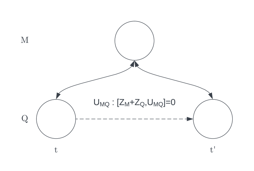
Figure 1: Pictorial representation of the temporal witness of non-classicality. $Q$ is the probe and $M$ is the system being assessed for non-classicality by testing its ability to induce a non-trivial quantum-coherent evolution of $Q$, conserving the quantity $Z_{M}+Z_{Q}$.

This condition requires $\left[U_{MQ},Z_{M}+Z_{Q}\right]=0$. If $M$ just has one classical variable $Z_{M}$, only Hamiltonians of the form $\alpha Z_{Q}+\beta Z_{M}+\gamma Z_{Q}Z_{M}$ are allowed, where $\alpha,\beta,\gamma$ are real-valued. These Hamiltonians cannot perform the witnessing task, of making $Z_{Q}$ unsharp from an initial condition where it is sharp on $Q$ [21]. Hence if the witnessing task can be realised by $M$, and the assumptions are satisfied, $M$ must have an extra, non-commuting variable – thus being non-classical, see Fig.1.

In the exciton transfer scenario, the quantum controllable system $Q$ is a single photon exciting the polymer at $t_{0}$, while the system $M$ is the exciton. The witnessing task is the quantum coherent evolution of the photon, mediated by the exciton $M$ that is created on the polymer when the photon $Q$ is absorbed. The conservation of the global energy of the photon-exciton system ensures that assumption (i) is satisfied. This scenario interestingly corresponds closely to experiments on exciton transfer in polydiacetylene, see e.g. [22].

III A qubit model for the exciton transfer

We shall now propose a quantum model to describe how the witnessing task can be performed even in a noisy environment, thus providing a scheme to experimentally test non-classicality in a macroscopic bio-polymer. This model shall illustrate the coherent evolution under energy conservation, thus implementing the temporal witness of non-classicality.

We shall consider a polymer whose $N$ monomers are described as a 1-d qubit chain. In the Heisenberg picture, each monomer $M_{j}$ is described by its components $\{X_{j},Y_{j},Z_{j}\}$, $j=1,...,N$, satisfying the Pauli algebra, where ${Z_{j}}$ is the computational basis. We introduce the raising and lowering operators for each monomer, $\sigma^{\pm}_{j}=X_{j}\pm iY_{j}$, to describe them with the operators $\{\sigma^{+}_{j},\sigma^{-}_{j},Z_{j}\}$.

The chain’s initial state is:

$$\rho_{S}=|{00...0}\rangle\langle{00...0}|$$ (1)

as no excitation has been created yet.

Creation of an exciton.– A photon $Q$ creates an exciton on the chain. It is initially localised on the first monomer of the chain. Its quantum observables are ${X^{p}_{j},Y^{p}_{j},Z^{p}_{j}}$, $\alpha^{\pm}_{j}=X^{p}_{j}\pm iY^{p}_{j}$ and its initial state is:

$$\rho_{p}=|{10...0}\rangle\langle{10...0}|.$$ (2)

Once the photon interacts with the first monomer, its degree of freedom is swapped with the degree of freedom of the monomer itself, so that:

$${}^{0}\rho_{S}=Tr_{\rho_{p}}[\textsc{swap}_{M_{1},p}\rho_{S}\otimes\rho_{p}\textsc{swap}^{\dagger}_{M_{1},p}]=|{10...0}\rangle\langle{10...0}|\;.$$ (3)

Now the exciton is localised on the first monomer of the chain. We focus on the single exciton regime, i.e., the probability of creating a second exciton in the chain is negligible, [22]. Crucially, the conservation law is satisfied by the first step of the model: $\left[\textsc{swap}_{M_{1},p},\sum_{j=1}^{N}{Z_{j}}+Z_{p}\right]=0$.

Exciton Dynamics and Environment.– We describe the exciton propagation with an XX-Hamiltonian [23]:

$$H_{XX} =\frac{1}{2}\sum_{n=1}^{N}J_{n}\left(X_{n}X_{n+1}+Y_{n}Y_{n+1}\right)-\sum_{n=1}^{N}{B_{n}Z_{n}}$$ (4)

$$=\frac{1}{4}\sum_{n=1}^{N}J_{n}\left(\sigma^{+}_{n}\sigma^{-}_{n+1}+\sigma^{-}_{n}\sigma^{+}_{n+1}\right)-\sum_{n=1}^{N}{B_{n}Z_{n}}$$ (5)

where $J_{n},B_{n}\in\mathbb{R}$ $\forall\ n=1,...,N$. Notably, this model can capture different polymers simply by changing $J_{n}$ and $B_{n}$. Thus it can be easily extended to other phenomena, like anisotropies in the polymer, next-nearest neighbours coupling and multiple dimensions. Moreover, since $\left[H_{XX},\sum_{j=1}^{N}{Z_{j}}\right]=0$, this step of the model satisfies the conservation law too, as requrired by the witness.

To be realistic, one must also take into account the environment, which induces decoherence. Here we shall model the environment as a thermal bath, using a quantum homogeniser [24]. This is a reservoir of $M$ qubits that when suitably initialised can be used to prepare a system qubit in any quantum state, to an arbitrarily high precision, improving as we increase $M$.

Initially the qubits in the reservoir are all prepared in the same maximally mixed state, so that:

$${}^{0}\xi=\bigotimes^{M}_{j=1}{{}^{0}\xi_{j}}=\left[\frac{1}{2}(|{0}\rangle\langle{0}|+|{1}\rangle\langle{1}|)\right]^{\otimes M}.$$ (6)

The decoherence is modelled by the interaction between the system and the reservoir, via the partial swap $\textsc{pswap}=\cos{\eta}\ \mathbf{I}+i\sin{\eta}\ \textsc{swap}$, where $\mathbf{I}$ is the identity operator on a two-qubit Hilbert space and $\eta$ is the interaction strength between the system and the reservoir, or the decoherence strength. This unitary satisfies the conservation law, because $\left[\textsc{pswap},\sum_{j=1}^{N}{Z_{j}}+\sum_{l=1}^{M}{Z_{l}}\right]=0$.

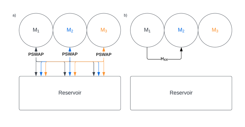
Figure 2: Schematic representation of the protocol: a) Decoherence phase; b) Transfer phase.

The protocol for the decohered exciton transfer works as follows. At each iteration of the protocol $k$, with $k=1,...,N$, each monomer $M_{j}$, $j=1,...,N$, undergoes the homogenisation process with the $M$ qubits/phonons in the reservoir. This is the decoherence phase, see Fig.2a). When the homogenisation has been performed on all the monomers, i.e, the decoherence round has ended, the monomer $M_{k}$ transfers its quantum state to the monomer $M_{k+1}$. This is the transfer phase of the protocol, see Fig.2b). After the transfer phase, the protocol can be repeated for the $k+1$-th iteration. This explains the notation: the upper script $0$ in ${}^{0}\rho_{S}$ and ${}^{0}\xi$ refers to the state of the system and the reservoir, respectively, before the protocol begins, at $k=0$.

We shall introduce two different models for the reservoir in this scenario: (1) Markov Environment: we re-initialise the quantum homogeniser in the maximally mixed state ${}^{0}\xi$ whenever a new monomer is involved in the decoherence phase of the protocol, at every iteration; (2) Non-Markov Environment: the reservoir is never re-initialised, neither when a new monomer enters the decoherence phase nor when a new iteration of the protocol begins.

Exciton recombination.– At the end of the $N^{th}$ iteration, we model recombination by swapping again the spatial degrees of freedom of the polymer and that of the photon. The witnessing task is performed if the photon is quantum coherently delocalised on every monomer of the chain:

$$\rho_{p}= p_{0}|{00...0}\rangle\langle{00...0}|+p_{1}|{10...0}\rangle\langle{10...0}|$$

$$+p_{2}|{01...0}\rangle\langle{01...0}|+...+p_{N}|{00...1}\rangle\langle{00...1}|;$$ (7)

This dynamics provides the coherent evolution required by the temporal witness of non-classicality.

If the photon is capable of interfere once re-emitted, the witnessing task is succesfully performed. Assuming the conservation law of the additive quantity $\sum_{j=1}^{N}{Z_{j}}+\sum_{l=1}^{M}{Z_{l}}+Z_{p}$, the witness allow us to conclude that the exciton, and hence the biopolymer, is non-classical.

III.1 Markovian Environment

Here we derive the final state of the photon in the framework of a Markovian environment. This scenario is equivalent to having a different reservoir per monomer at each iteration of the protocol. Every reservoir is initialised in the maximally mixed state in Eq.6, while the polymer is initially in the state in Eq. 3. As described in Appendix A, the final state of the photon after the exciton recombination (in the simpler $N=M=3$ case) is:

$${}^{3}\rho_{p}= \left[{{}^{3}\rho_{p_{1}}}\otimes{{}^{3}\rho_{p_{2}}}+itJ_{1}\cos^{18}{\eta}\left(\alpha^{+}_{1}\alpha^{-}_{2}-\alpha^{-}_{1}\alpha^{+}_{2}\right)\right.$$

$$\left.-t^{2}B_{2}\left(\alpha^{+}_{1}\alpha^{-}_{2}+\alpha^{-}_{1}\alpha^{+}_{2}\right)\right]\otimes{{}^{3}\rho_{p_{3}}}$$

$$-t^{2}J_{1}J_{2}\cos^{18}{\eta}\left(Z_{2}+\cos^{12}{\eta}\right)\left(\alpha^{+}_{1}\alpha^{-}_{3}+\alpha^{-}_{1}\alpha^{+}_{3}\right)$$ (8)

where ${{}^{3}\rho_{p_{j}}}$ is the density matrix of the photon localised on the monomer $M_{j}$ at the $k=3$ iteration of the protocol.

III.2 Non-Markovian Environment

In the Non-Markov environment, the reservoir evolves with the polymer. This is the Non-Markovian feature of the model (different from other models, e.g. in [25]): the state of each reservoir qubit has “memory”, and it cannot be re-initialised at every iteration.

We assume for simplicity that the system is an $N=3$ monomer chain and the reservoir is made of $M=3$ qubits. We initialise the reservoir in the maximally mixed state (Eq.6) and the polymer in the state Eq.3. As shown in Appendix B the final state of the photon is:

$${}^{3}\rho_{p}={{}^{3}\rho_{p_{1}}}\otimes{{}^{3}\rho_{p_{2}}}\otimes{{}^{3}\rho_{p_{3}}}$$

$$+itJ_{1}\left[F(\eta)+2itB_{2}G(\eta)\right]\left(\alpha^{+}_{1}\alpha^{-}_{2}-\alpha^{-}_{1}\alpha^{+}_{2}\right)\otimes{{}^{3}\rho_{p_{3}}}$$

$$+itJ_{1}\left[G(\eta)+2itB_{2}F(\eta)\right]\left(\alpha^{+}_{1}\alpha^{-}_{2}+\alpha^{-}_{1}\alpha^{+}_{2}\right)\otimes{{}^{3}\rho_{p_{3}}}$$

$$-\frac{1}{2}t^{2}J_{1}J_{2}\left(Z_{2}+s(\eta)\right)\left[F(\eta)\left(\alpha^{+}_{1}\alpha^{-}_{3}+\alpha^{-}_{1}\alpha^{+}_{3}\right)\right.$$

$$\left.+G(\eta)\left(\alpha^{+}_{1}\alpha^{-}_{3}-\alpha^{-}_{1}\alpha^{+}_{3}\right)\right]$$ (9)

where $F(\eta),G(\eta)$ and $s(\eta)$ are defined in Appendix B and ${{}^{3}\rho_{p_{j}}}$ is the density matrix of the photon localised over the monomer $M_{j}$ at the $k=3$ iteration.

IV Discussion

We shall now compare the two states for the Markov (Eq.8) and Non-Markov (Eq.9) environments.

In the weak coupling limit, in both the scenarios, the exciton mediates a coherent delocalisation of the photon over the polymer. Hence the witnessing task is successfully achieved, even in the presence of decoherence. Using the temporal witness of non-classicality, one can conclude that the exciton mediating the photon coherent delocalisation is non-classical, and so the process governing its transfer along the polymer must be non-classical itself. The model explains why, despite decoherence, a coherent delocalisation of the exciton over the chain is still possible: the interactions between the monomers mitigate the decoherence, preventing ${}^{k}\rho_{S}$ from becoming an eigenstate of $H_{XX}$ in Eq.5.

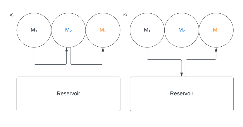
Figure 3: Schematic view of the coherent hopping mechanisms: a) via intermediate monomers; b) via reservoir.

Interestingly, at every time step, the exciton can face three different scenarios: (1) It can remain localised on the monomer preceeding that involved in the transfer phase, as suggested by the coefficients $B_{j}$; (2) It can (coherently) hop on to the next monomer. This can occur via two mechanisms: (2.1) Via the intermediate monomers, see Fig.3a). (2.2) Via the reservoir, see Fig.3b). We notice that the preceding monomers are not involved here: the environment is solely responsible for the quantum coherent delocalisation of the exciton.

The difference between a Markov and a Non-Markov environment therefore lies in the amount of coherence maintained by the qubits. Such coherence (i) creates, at every iteration, a second “hopping term” between the two monomers involved in the transfer phase, shifted by a phase factor $e^{i\pi}$; (ii) reshapes the probabilities for the coherent delocalisation of the exciton over the polymer.

Consider now the coefficients of the terms describing the aforementioned mechanisms.

	Markov	$F(\eta)$	$G(\eta)$
$M_{1}\leftrightarrow Q_{1}$	0.961	0.961	$i9.7\cdot 10^{-4}$
$M_{1}\leftrightarrow Q_{2}$	0.951	0.951	$i9.3\cdot 10^{-4}$
$M_{1}\leftrightarrow Q_{3}$	0.942	0.942	$i1.3\cdot 10^{-3}$
$M_{2}\leftrightarrow Q_{1}$	0.932	0.932	$i3.7\cdot 10^{-5}$
$M_{2}\leftrightarrow Q_{2}$	0.923	0.923	$i9.4\cdot 10^{-4}$
$M_{2}\leftrightarrow Q_{3}$	0.914	0.914	$-i8.3\cdot 10^{-4}$

Table 1: Coefficients hopping terms via chain with $\eta=0.1$ at every step of the decoherence phase of $k=2$ iteration.

Figure 4: Coefficients $F(\eta)$ (blue) and $\cos^{18}{\eta}$ (orange) at the end of $k=2$ iteration

Figure 5: Coefficients $F(\eta)$ (blue) and $G(\eta)$ (orange) at the end of $k=2$ iteration.

Table 1 shows the coefficients of the terms describing the coherent delocalisation of the exciton via the chain (mechanism (2.1)), with a decoherence parameter $\eta=0.1$. $F(\eta)$ and the coefficient in the Markov scenario are the same at every step of the protocol. This holds true for all the values of $\eta$ in the weak coupling regime, as shown in Fig.4. Moreover, $G(\eta)$ appears to be very small, almost negligible. Interestingly, if one sets $G(\eta)=0$, the two final states in Eq.8 and Eq.9, although very different in their analytical expressions, have the same numerical values in the weak coupling regime. This can be generalised to all other $\eta$, see Fig.5. Thus, the effect of $G(\eta)$, in the Non-Markovian environment, is practically negligible for the mechanism (2.1): small values of $\eta$ makes the interaction with the environment very unlikely, therefore it cannot mediate the exciton transport along the polymer. This elucidates why the coefficient $F(\eta)$ has the same value of its Markovian counterpart at every step of the protocol.

Moreover, for some values of $\eta$, both $F(\eta)$ and $G(\eta)$ are vanishing: the hopping via chain is prevented by the strong coupling with the environment. The effect of decoherence is so strong that the monomers lose coherence as soon as they interact with the environment. They effectively become equivalent to classical bits and not capable of quantum-coherently transmitting the exciton anymore.

Figure 6: Coefficients $s(\eta)$ (blue) and $\cos^{12}(\eta)$ (orange) at the end of $k=2$ iteration.

Considering the role played by the non-Markovian environment in (2.2), i.e., the hopping mechanism via the reservoir, the same argument as before applies, focusing on the coefficients $s(\eta)$ and $\cos^{12}{\eta}$. They have almost the same numerical values as in the weak coupling regime, as one can see in Fig.6. As soon as the coupling with the environment increases, entering the strong coupling regime, the hopping via reservoir becomes impossible with a Markovian environment, but it is still possible with a Non-Markov environment. Informally, one can say that the coherence “stored” by a Non-Markov environment is then used by the polymer for the quantum coherent delocalisation of the exciton. Hence the non-Markovian environment becomes crucial for the energy transfer in the strong coupling regime, as no other hopping mechanism is allowed. This may provide an explanation for why polymer vibrations may be relevant in exciton-mediated transport phenomena, such as light harvesting [26, 27, 28, 29, 30].

V Conclusions

We have proposed a novel experimental scheme to witness non-classicality in the exciton transfer on a bio-polymer, using a photonic quantum probe. This witness is subtly different from other ones, e.g. [31, 32], as it investigates an intrinsic, more general, property of the biological system itslef, rather than of the specific process. This witness has the appeal of being very broadly applicable and of relying only on a few general assumptions: energy conservation and the formalism of quantum theory. One in fact could relax the latter and recast this witness of non-classicality in the information-theoretic framework known as constructor theory of information [33]. This dynamics-independent approach would achieve full generality in our argument, giving interesting insights regarding possible physical reasons why biological systems must be non-classical [34]. We shall explore this in a forthcoming paper.

We have also provided a qubit model to describe the exciton transfer, together with an analysis of decoherence, in the Markovian and non-Markovian regime. This model is very general too, and could be adopted to describe a number of existing quantum biology results, [13, 35, 36].

The role of a Non-Markovian environment in the witnessing task becomes essential in the strong coupling regime: the only way for the witnessing task to be possible when $\eta\geq 1.571$ is to rely on the interaction of the polymer with its own Non-Markovian environment. This is due to the fact that the reservoir has memory of the occurred process and maintains coherence throughout it. Instead, in a weak coupling scenario, the witnessing task is possible independently of the Markovianity of the reservoir. This conclusion is intuitively pleasing since in the strong coupling regime the separation between the system and environment becomes nonphysical and it is more appropriate to think of the environment as being part of the system.

The generality of our witnessing scheme makes it an ideal candidate for designing new experiments in quantum biology, to pin down conclusively the role of quantum effects in exciton transfer and other energy transfer processes. We leave the development of this research to future work.

Acknowledgements   We thank Simone Rijavec, Maria Violaris, Mattheus Burkhard, Antonio Pantelias Garcés, Virginia Tsiouri and Tristan Farrow for sharp comments and fruitful discussions on this manuscript. This research was made possible through the generous support of the Gordon and Betty Moore Foundation. G.D. thanks the Clarendon Fund and the Oxford-Thatcher Graduate Scholarship for supporting this research.

Appendix A A. Markovian Environment: analytical derivation of Eq.8

In this Appendix, we will analytically derive Eq.8 and the general state for $N$ monomers and $M$ reservoir qubits, going iteration by iteration in the protocol and providing the final state of the emitted photon after the recombination of the exciton on the polymer. The setup is the very same discussed in the Section Markovian Environment.

First iteration $k=1$.– We start with the polymer being in the state described by the density matrix in Eq. 3. At this stage, the state of the system is separable, so that we can write:

$${}^{0}\rho_{S}={{}^{0}\rho_{S_{1}}}\otimes{{}^{0}\rho_{S_{2}}}\otimes...\otimes{{}^{0}\rho_{S_{N}}}$$ (10)

being ${}^{0}\rho_{S_{j}}$, $j=1,...,N$, the reduced density matrix of the monomer $M_{j}$ before the beginning of the homogenisation process in the $k=1$ iteration. It is convenient to write the single monomer density matrices using the Bloch vector representation:

$${}^{0}\rho_{S_{1}}=\frac{1}{2}\left(\mathbf{I}+{{}^{0}\vec{s}_{1}}\cdot\vec{\sigma}\right)=\frac{1}{2}\left(\mathbf{I}-Z_{1}\right)$$ (11)

where $\sigma$ is the vector of Pauli operators and the initial condition for the first monomer of the chain is ${}^{0}\vec{s}_{1}=-\hat{z}$ since it is excited by the photon, so it is in the state $|{1}\rangle$. Similarly:

$${}^{0}\rho_{S_{j}}=\frac{1}{2}\left(\mathbf{I}+{{}^{0}\vec{s}_{j}}\cdot\vec{\sigma}\right)=\frac{1}{2}\left(\mathbf{I}+Z_{j}\right),\ \ \ j=2,...,N$$ (12)

where the initial conditions are ${}^{0}\vec{s}_{j}=+\hat{z}$ because all the remaining monomers are not excited by the photon at the beginning. Recall in fact that our photon is initially spatially localised on the first monomer. Moving now to the reservoir qubits, we can adopt for them too the Bloch vector representation:

$${}^{0}\xi_{j}=\frac{1}{2}\left(\mathbf{I}+{{}^{0}\vec{r}_{j}}\cdot\vec{\sigma}\right)=\frac{1}{2}\left(\mathbf{I}\right),\ \ \ j=1,...,M$$ (13)

where ${}^{0}\vec{r}_{j}=0$ because we initialise all the qubits in the reservoir in the maximally mixed state.

We can now start with the decoherence phase of the $k=1$ iteration of the protocol, i.e., the first round of homogenisation for the polymer. We start with the first, excited, monomer. It interacts with the first qubit in the reservoir:

$${}^{1}\rho^{(1)}_{S_{1}} =Tr_{{{}^{0}\xi_{1}}}\left[\textsc{pswap}_{{{}^{0}\rho_{S_{1}}},{{}^{0}\xi_{1}}}{\left({{}^{0}\rho_{S_{1}}}\otimes{{}^{0}\xi_{1}}\right)}\textsc{pswap}^{\dagger}_{{{}^{0}\rho_{S_{1}}},{{}^{0}\xi_{1}}}\right]$$

$$=\frac{1}{2}\left(\mathbf{I}+{{}^{1}\vec{s}^{(1)}_{1}}\cdot\vec{\sigma}\right)=\frac{1}{2}\left(\mathbf{I}-\cos^{2}{\eta}\ Z_{1}\right)$$ (14)

where the Bloch vector ${{}^{1}\vec{s}^{(1)}_{1}}$ evolves as:

$${}^{1}\vec{s}^{(1)}_{1} =\cos^{2}{\eta}\ {{}^{0}\vec{s}_{1}}+\sin^{2}{\eta}\ {{}^{0}\vec{r}_{1}}-\cos{\eta}\sin{\eta}\left({{}^{0}\vec{r}_{1}}\times{{}^{0}\vec{s}_{1}}\right)$$

$$=-\cos^{2}{\eta}\ \hat{z}.$$ (15)

This means that the decoherence process, at this stage of the protocol, shrinks the length of the monomer’s Bloch vector of a factor $\cos^{2}{\eta}$ for every qubit in the reservoir. We can easily generalise this process to the $M^{th}$ interaction with the reservoir, to have:

$${}^{1}\rho^{(M)}_{S_{1}}=\frac{1}{2}\left(\mathbf{I}+{{}^{1}\vec{s}^{(M)}_{1}}\cdot\vec{\sigma}\right)=\frac{1}{2}\left(\mathbf{I}-\cos^{2M}{\eta}\ Z_{1}\right)$$ (16)

where:

$${}^{1}\vec{s}^{(M)}_{1} =\cos^{2}{\eta}\ {{}^{1}\vec{s}^{(M-1)}_{1}}+\sin^{2}{\eta}\ {{}^{0}\vec{r}_{M}}$$

$$\ \ \ -\cos{\eta}\sin{\eta}\left({{}^{0}\vec{r}_{M}}\times{{}^{0}\vec{s}^{(M-1)}_{1}}\right)$$

$$=\cos^{2}{\eta}(-\cos^{2(M-1)}{\eta})\hat{z}=-\cos^{2M}{\eta}\ \hat{z}.$$ (17)

This concludes the decoherence phase for the first monomer.

We move now to the second monomer. Since we are in the Markov environment scenario, we can initialise again the reservoir to a collection of $M$ qubits prepared in the maximally mixed state, or equivalently we can say that the second monomer interacts with a different environment, equally built and prepared. This allows us to use the very same results we got for the decoherence phase of the first monomer, with the only difference that the initial condition for the second monomer $M_{2}$ is given by ${}^{0}\vec{s}_{2}=+\hat{z}$, since it is not excited by the photon. We will thus have:

$${}^{1}\rho^{(M)}_{S_{2}}=\frac{1}{2}\left(\mathbf{I}+{{}^{1}\vec{s}^{(M)}_{2}}\cdot\vec{\sigma}\right)=\frac{1}{2}\left(\mathbf{I}+\cos^{2M}{\eta}\ Z_{2}\right)$$ (18)

where:

$${}^{1}\vec{s}^{(M)}_{2} =\cos^{2}{\eta}\ {{}^{1}\vec{s}^{(M-1)}_{2}}+\sin^{2}{\eta}\ {{}^{0}\vec{r}_{M}}$$

$$\ \ \ -\cos{\eta}\sin{\eta}\left({{}^{0}\vec{r}_{M}}\times{{}^{0}\vec{s}^{(M-1)}_{2}}\right)$$

$$=\cos^{2}{\eta}(+\cos^{2(M-1)}{\eta})\hat{z}=+\cos^{2M}{\eta}\ \hat{z}.$$ (19)

The same reasoning can be applied to all the remaining monomers in the chain, so that at the end of the decoherence phase for the $k=1$ iteration of the protocol our monomers will be in the states:

$$\begin{cases}{}^{1}\rho^{(M)}_{S_{1}}=\frac{1}{2}\left(\mathbf{I}-\cos^{2M}{\eta}\ Z_{1}\right)\\ {}^{1}\rho^{(M)}_{S_{j}}=\frac{1}{2}\left(\mathbf{I}+\cos^{2M}{\eta}\ Z_{j}\right)\ \ \ \ \ j=2,...,N\end{cases}$$ (20)

and the state of the polymer:

$${}^{1}\rho_{S}={{}^{1}\rho^{(M)}_{S_{1}}}\otimes{{}^{1}\rho^{(M)}_{S_{2}}}\otimes...\otimes{{}^{1}\rho^{(M)}_{S_{N}}}.$$ (21)

The first iteration of the protocol ends with the transfer phase involving the monomers $M_{1}$ and $M_{2}$. This is described by the unitary ($\hbar=1$ from now on):

$$U=e^{-iH_{XX}t}$$ (22)

where $H_{XX}$ is the XX Hamiltonian in Eq.5. We find:

$${}^{1}\rho_{S_{1,2}}=U\left({{{}^{1}\rho^{(M)}_{S_{1}}}\otimes{{}^{1}\rho^{(M)}_{S_{2}}}}\right)U^{\dagger}$$ (23)

which, at first order in $t$, gives:

$${}^{1}\rho_{S_{1,2}}={{}^{1}\rho^{(M)}_{S_{1}}}\otimes{{}^{1}\rho^{(M)}_{S_{2}}}+\frac{1}{4}itJ_{1}\cos^{2M}{\eta}\left(\sigma^{+}_{1}\sigma^{-}_{2}-\sigma^{-}_{1}\sigma^{+}_{2}\right).$$ (24)

All in all, the state of the polymer after the $k=1$ iteration of the protocol, which will in turn be the initial state for the $k=2$ iteration, is:

$${}^{2}\rho_{S}={{}^{1}\rho_{S_{1,2}}}\otimes{{}^{1}\rho^{(M)}_{S_{j}}}^{\otimes(N-2)}\ \ \ j=3,...,N.$$ (25)

Second iteration $k=2$.– Since we are dealing with the Markov environment, before beginning with the decoherence phase we must initialise again the reservoir in the state ${}^{0}\xi$ of Eq.6. The state of the polymer, instead, is the one in Eq.25, where the monomers $M_{1}$ and $M_{2}$ are entangled. In this case, the homogenisation process will be performed locally on both $M_{1}$ and $M_{2}$. The entangled state ${}^{1}\rho_{S_{1,2}}$ in Eq.24 can be divided in a separable and a non-separable part, which we can discuss separately.

The separable part of Eq.24 will evolve as described in the $k=1$ iteration of the protocol, with the only difference that now the initial conditions for the two monomers $M_{1}$ and $M_{2}$ are given by ${}^{1}\vec{s}^{(M)}_{1}$ in Eq.17 and ${}^{1}\vec{s}^{(M)}_{2}$ in Eq.19. After $M$ interactions with the reservoir, we will have;

$$\begin{cases}{}^{2}\rho^{(M)}_{S_{1}}=\frac{1}{2}\left(\mathbf{I}-\cos^{(4M)}{\eta}Z_{1}\right)\\ {}^{2}\rho^{(M)}_{S_{2}}=\frac{1}{2}\left(\mathbf{I}+\cos^{(4M)}{\eta}Z_{2}\right)\end{cases}$$ (26)

The non-separable part is the most interesting to explore. We shall call it ${}^{1}\rho^{non-sep}_{S_{1,2}}$ Let us start with the first monomer being involved in the decoherence phase. Interacting with the first qubit of the reservoir, we find:

$${}^{1}\rho^{non-sep,(1)}_{S_{1,2}}=\frac{1}{2}itJ_{1}\cos^{2M}{\eta}\cos^{2}{\eta}\left(\sigma^{+}_{1}\sigma^{-}_{2}-\sigma^{-}_{1}\sigma^{+}_{2}\right)$$ (27)

so that, after the interaction with the remaining $M-1$ qubits in the reservoir, ${}^{1}\rho^{non-sep}_{S_{1,2}}$ will be:

$${}^{1}\rho^{non-sep,(M)}_{S_{1,2}}=2^{(M-2)}itJ_{1}\cos^{4M}{\eta}\left(\sigma^{+}_{1}\sigma^{-}_{2}-\sigma^{-}_{1}\sigma^{+}_{2}\right).$$ (28)

The same reasoning can be applied when the second monomer $M_{2}$ undergoes the decoherence phase. After the interaction with the $M^{th}$ qubit in the reservoir, the final state of the non-separable part of ${}^{1}\rho_{S_{1,2}}$ is:

$${}^{1}\rho^{non-sep,(2M)}_{S_{1,2}}=2^{(2M-2)}itJ_{1}\cos^{6M}{\eta}\left(\sigma^{+}_{1}\sigma^{-}_{2}-\sigma^{-}_{1}\sigma^{+}_{2}\right).$$ (29)

All in all, the entangled state in Eq.24 after the decoherence phase of the $k=2$ iteration becomes (re-scaling the coefficient properly to remove the constant numeric factors):

$${}^{2}\rho^{(M)}_{S_{1,2}}={{}^{2}\rho^{(M)}_{S_{1}}}\otimes{{}^{2}\rho^{(M)}_{S_{2}}}+itJ_{1}\cos^{6M}{\eta}\left(\sigma^{+}_{1}\sigma^{-}_{2}-\sigma^{-}_{1}\sigma^{+}_{2}\right),$$ (30)

while the remaining $N-2$ monomers, not being involved in the quantum state transfer, evolve as described in the previous iteration:

$${}^{2}\rho^{(M)}_{S_{j}}=\frac{1}{2}\left(\mathbf{I}+\cos^{4m}{\eta}Z_{j}\right)\ \ \ \ j=3,...,N.$$ (31)

We move now to the transfer phase of the $k=2$ iteration, involving the monomers $M_{2}$ and $M_{3}$. Applying again the unitary in Eq.22 to first order in $t$, we find:

$${}^{2}\rho_{S_{1,2,3}}=U\left({{{}^{2}\rho^{(M)}_{S_{1,2}}}\otimes{{}^{2}\rho^{(M)}_{S_{2}}}}\right)U^{\dagger}=$$

$$=\left[{{}^{2}\rho^{(M)}_{S_{1}}}\otimes{{}^{2}\rho^{(M)}_{S_{2}}}+itJ_{1}\cos^{6M}{\eta}\left(\sigma^{+}_{1}\sigma^{-}_{2}-\sigma^{-}_{1}\sigma^{+}_{2}\right)\right.$$

$$\left.-t^{2}B_{2}\left(\sigma^{+}_{1}\sigma^{-}_{2}+\sigma^{-}_{1}\sigma^{+}_{2}\right)\right]\otimes{{}^{2}\rho^{(M)}_{S_{3}}}$$

$$-t^{2}J_{1}J_{2}\cos^{6M}{\eta}\left(Z_{2}+\cos^{4M}{\eta}\right)\left(\sigma^{+}_{1}\sigma^{-}_{3}+\sigma^{-}_{1}\sigma^{+}_{3}\right).$$ (32)

We can now summarise the outcome of the $k=2$ iteration of the protocol, which in turn is the initial state of the iteration $k=3$. The state of the polymer will be:

$${}^{3}\rho_{S}={{}^{2}\rho_{S_{1,2,3}}}\otimes{{}^{2}\rho^{(M)}_{S_{j}}}^{\otimes(N-3)}\ \ \ j=4,...,N.$$ (33)

$N^{th}$ iteration $k=N$ and recombination.– Understood the way in which our decoherence map works for the decoherence phase and what mechanisms are involved in the transfer phase, we can easily generalise the protocol to the very last step: the exciton arrived to the last but one monomer in the chain and, after the last decoherence phase, is transmitted to the monomer $M_{N}$; it is at this stage that the exciton will finally recombine on the polymer, emitting again a single photon. The final state of the photon will thus be:

$${}^{N}\rho_{p}=\left[{{}^{N}\rho_{p_{1}}}\otimes{{}^{N}\rho_{p_{2}}}+itJ_{1}\cos^{[2+4(N-2)]M}{\eta}\left(\alpha^{+}_{1}\alpha^{-}_{2}-\alpha^{-}_{1}\alpha^{+}_{2}\right)-t^{2}B_{2}\cos^{4(N-3)M}{\eta}\left(\alpha^{+}_{1}\alpha^{-}_{2}+\alpha^{-}_{1}\alpha^{+}_{2}\right)\right]{{}^{N}\rho_{p_{3}}}\otimes...\otimes{{{}^{N}\rho_{p_{M}}}}$$

$$-t^{2}J_{1}J_{2}\cos^{[2+4(N-2)]M}{\eta}\left(\cos^{(N-3)2M}{\eta}Z_{2}+\cos^{4M}{\eta}\right)\left[\left(\alpha^{+}_{1}\alpha^{-}_{3}+\alpha^{-}_{1}\alpha^{+}_{3}\right)+itB_{3}\left(\alpha^{+}_{1}\alpha^{-}_{3}-\alpha^{-}_{1}\alpha^{+}_{3}\right)\right]{{}^{N}\rho_{p_{4}}}\otimes...\otimes{{{}^{N}\rho_{p_{M}}}}$$

$$+...+(i)^{2N-3}t^{N-2}J_{1}J_{2}...J_{N-1}\cos^{[2+4(N-2)]M}{\eta}\left(\cos^{(N-3)2M}{\eta}Z_{2}+\cos^{4M}{\eta}\right)...\left(Z_{N}+\cos^{2(N-1)M}{\eta}\right)\cdot$$

$$\cdot\left[\left(\alpha^{+}_{1}\alpha^{-}_{N}+(-1)^{2N-3}\alpha^{-}_{1}\alpha^{+}_{N}\right)+itB_{N}\left(\alpha^{+}_{1}\alpha^{-}_{N}+(-1)^{2N-2}\alpha^{-}_{1}\alpha^{+}_{N}\right)\right].$$ (34)

where ${{}^{N}\rho_{p_{j}}}$ is the density matrix of the photon localised over the monomer $M_{j}$ at the $k=N$ iteration of the protocol.

Appendix B B. Non-Markovian Environment: analytical derivation of Eq.9

Here we will detail the procedure leading to Eq.9 and provide some useful generalisation to compute the needed coefficients for larger systems. The setup is the very same discussed in the Section Non-Markovian Environment.

First iteration $k=1$.– We start again with the polymer being in the state described by the density matrix in Eq. 3:

$${}^{0}\rho_{S}={{}^{0}\rho_{S_{1}}}\otimes{{}^{0}\rho_{S_{2}}}\otimes{{}^{0}\rho_{S_{3}}}$$ (35)

being ${}^{0}\rho_{S_{j}}$, $j=1,...,3$, the reduced density matrix of the monomer $M_{j}$ before the beginning of the homogenisation process in the $k=1$ iteration. We write the single monomer density matrices using the Bloch vector representation:

$${}^{0}\rho_{S_{1}}=\frac{1}{2}\left(\mathbf{I}+{{}^{0}\vec{s}_{1}}\cdot\vec{\sigma}\right)=\frac{1}{2}\left(\mathbf{I}-Z_{1}\right)$$ (36)

where $\sigma$ is the vector of Pauli operators and the initial condition for the first monomer of the chain is ${}^{0}\vec{s}_{1}=-\hat{z}$ since it is excited by the photon, so it is in the state $|{1}\rangle$. Similarly:

$${}^{0}\rho_{S_{j}}=\frac{1}{2}\left(\mathbf{I}+{{}^{0}\vec{s}_{j}}\cdot\vec{\sigma}\right)=\frac{1}{2}\left(\mathbf{I}+Z_{j}\right),\ \ \ j=2,3$$ (37)

where the initial conditions are ${}^{0}\vec{s}_{j}=+\hat{z}$ because all the remaining monomers are not excited by the photon at the beginning. Recall in fact that our photon is initially spatially localised on the first monomer. Moving now to the reservoir qubits, we can adopt for them too the Bloch vector representation:

$${}^{0}\xi_{j}=\frac{1}{2}\left(\mathbf{I}+{{}^{0}\vec{r}_{j}}\cdot\vec{\sigma}\right)=\frac{1}{2}\left(\mathbf{I}\right),\ \ \ j=1,...,3$$ (38)

where ${}^{0}\vec{r}_{j}=0$ because we initialise all the qubits in the reservoir in the maximally mixed state.

We can now start with the decoherence phase of the $k=1$ iteration of the protocol, i.e., the first round of homogenisation for the polymer. We start with the first, excited, monomer. It interacts with the first qubit in the reservoir:

$${}^{1}\rho^{(1)}_{S_{1}} =Tr_{{{}^{0}\xi_{1}}}\left[\textsc{pswap}_{{{}^{0}\rho_{S_{1}}},{{}^{0}\xi_{1}}}{\left({{}^{0}\rho_{S_{1}}}\otimes{{}^{0}\xi_{1}}\right)}\textsc{pswap}^{\dagger}_{{{}^{0}\rho_{S_{1}}},{{}^{0}\xi_{1}}}\right]$$

$$=\frac{1}{2}\left(\mathbf{I}+{{}^{1}\vec{s}^{(1)}_{1}}\cdot\vec{\sigma}\right)=\frac{1}{2}\left(\mathbf{I}-\cos^{2}{\eta}\ Z_{1}\right)$$ (39)

where the Bloch vector ${{}^{1}\vec{s}^{(1)}_{1}}$ evolves as:

$${}^{1}\vec{s}^{(1)}_{1} =\cos^{2}{\eta}\ {{}^{0}\vec{s}_{1}}+\sin^{2}{\eta}\ {{}^{0}\vec{r}_{1}}-\cos{\eta}\sin{\eta}\left({{}^{0}\vec{r}_{1}}\times{{}^{0}\vec{s}_{1}}\right)$$

$$=-\cos^{2}{\eta}\ \hat{z}.$$ (40)

As before, the decoherence process on the first monomer has the effect of shrinking the length of its Bloch vector of a factor $\cos^{2}{\eta}$ for every qubit in the reservoir.

Here comes the difference with the previous scenario: since now the environment we’re dealing with is a Non-Markovian one, we have to store in the reservoir qubits the information about the interaction with the first monomer of the chain. Thus, we have also to compute the states of the reservoir qubits after the interaction with $M_{1}$:

$${}^{1}\xi^{{}^{\prime}}_{1} =Tr_{{{}^{0}\rho_{S_{1}}}}\left[\textsc{pswap}_{{{}^{0}\rho_{S_{1}}},{{}^{0}\xi_{1}}}{\left({{}^{0}\rho_{S_{1}}}\otimes{{}^{0}\xi_{1}}\right)}\textsc{pswap}^{\dagger}_{{{}^{0}\rho_{S_{1}}},{{}^{0}\xi_{1}}}\right]$$

$$=\frac{1}{2}\left(\mathbf{I}+{{}^{1}\vec{r}^{(1)}_{1}}\cdot\vec{\sigma}\right)=\frac{1}{2}\left(\mathbf{I}-\sin^{2}{\eta}\ Z_{1}^{res}\right)$$ (41)

where the Bloch vector ${{}^{1}\vec{r}^{(1)}_{1}}$ evolves as:

$${}^{1}\vec{r}^{(1)}_{1} =\sin^{2}{\eta}\ {{}^{0}\vec{s}_{1}}+\cos^{2}{\eta}\ {{}^{0}\vec{r}_{1}}+\cos{\eta}\sin{\eta}\left({{}^{0}\vec{r}_{1}}\times{{}^{0}\vec{s}_{1}}\right)$$

$$=-\sin^{2}{\eta}\ \hat{z}.$$ (42)

Since the reservoir qubits are all, at this stage, initialised in the maximally mixed state, we can easily generalise this process to the $3^{rd}$ interaction of the monomer $M_{1}$ with the reservoir, to have:

$${}^{1}\rho^{(3)}_{S_{1}}=\frac{1}{2}\left(\mathbf{I}+{{}^{1}\vec{s}^{(3)}_{1}}\cdot\vec{\sigma}\right)=\frac{1}{2}\left(\mathbf{I}-\cos^{6}{\eta}\ Z_{1}\right)$$ (43)

where:

$${}^{1}\vec{s}^{(3)}_{1} =\cos^{2}{\eta}\ {{}^{1}\vec{s}^{(2)}_{1}}+\sin^{2}{\eta}\ {{}^{0}\vec{r}_{3}}$$

$$\ \ \ -\cos{\eta}\sin{\eta}\left({{}^{0}\vec{r}_{3}}\times{{}^{0}\vec{s}^{(2)}_{1}}\right)$$

$$=\cos^{2}{\eta}(-\cos^{4}{\eta})\hat{z}=-\cos^{6}{\eta}\ \hat{z},$$ (44)

while the second and third reservoir qubit will be left in the states:

$${}^{1}\xi^{{}^{\prime}}_{2}=\frac{1}{2}\left(\mathbf{I}+{{}^{1}\vec{r}^{(1)}_{2}}\cdot\vec{\sigma}\right)=\frac{1}{2}\left(\mathbf{I}-\sin^{2}{\eta}\cos^{2}{\eta}\ Z_{2}^{res}\right)$$ (45)

and

$${}^{1}\xi^{{}^{\prime}}_{3}=\frac{1}{2}\left(\mathbf{I}+{{}^{1}\vec{r}^{(1)}_{3}}\cdot\vec{\sigma}\right)=\frac{1}{2}\left(\mathbf{I}-\sin^{2}{\eta}\cos^{4}{\eta}\ Z_{3}^{res}\right),$$ (46)

where:

$${}^{1}\vec{r}^{(1)}_{2} =\sin^{2}{\eta}\ {{}^{1}\vec{s}^{(1)}_{1}}+\cos^{2}{\eta}\ {{}^{0}\vec{r}_{2}}+\cos{\eta}\sin{\eta}\left({{}^{0}\vec{r}_{2}}\times{{}^{1}\vec{s}^{(1)}_{1}}\right)$$

$$=-\sin^{2}{\eta}\cos^{2}{\eta}\ \hat{z}$$ (47)

and

$${}^{1}\vec{r}^{(1)}_{3} =\sin^{2}{\eta}\ {{}^{1}\vec{s}^{(2)}_{1}}+\cos^{2}{\eta}\ {{}^{0}\vec{r}_{3}}+\cos{\eta}\sin{\eta}\left({{}^{0}\vec{r}_{3}}\times{{}^{1}\vec{s}^{(2)}_{1}}\right)$$

$$=-\sin^{2}{\eta}\cos^{4}{\eta}\ \hat{z}.$$ (48)

Now is the turn of the second monomer $M_{2}$ to undergo the decoherence phase. The qubits in the reservoir are now in the states ${{}^{1}\xi^{{}^{\prime}}_{j}}$, $j=1,2,3$. The process is the same described before, giving at the end of the interaction of $M_{2}$ with the third qubit in the reservoir:

$${}^{1}\rho^{(3)}_{S_{2}}=\frac{1}{2}\left[\mathbf{I}+\cos^{4}{\eta}\left(\cos^{2}{\eta}-3\sin^{4}{\eta}\right)\ Z_{2}\right]$$ (49)

and

$$\begin{cases}{}^{1}\xi^{{}^{\prime\prime}}_{1}=\frac{1}{2}\left[\mathbf{I}+\sin^{2}{\eta}\left(1-\cos^{2}{\eta}\right)\ Z_{1}^{res}\right]\\ {}^{1}\xi^{{}^{\prime\prime}}_{2}=\frac{1}{2}\left[\mathbf{I}+\sin^{2}{\eta}\left(\cos^{2}{\eta}-\cos^{4}{\eta}-\sin^{4}{\eta}\right)\ Z_{2}^{res}\right]\\ {}^{1}\xi^{{}^{\prime\prime}}_{3}=\frac{1}{2}\left[\mathbf{I}+\sin^{2}{\eta}\cos^{2}{\eta}\left(\cos^{2}{\eta}-\cos^{4}{\eta}-2\sin^{4}{\eta}\right)\ Z_{3}^{res}\right].\end{cases}$$ (50)

To conclude the decoherence phase for the $k=1$ iteration, we move now to the monomer $M_{3}$ considering the reservoir qubits in ${{}^{1}\xi^{{}^{\prime\prime}}_{j}}$, $j=1,2,3$:

$${}^{1}\rho^{(3)}_{S_{3}} =\frac{1}{2}\left\{[\mathbf{I}+\left[3\sin^{4}{\eta}\cos^{2}{\eta}\left(\cos^{2}{\eta}-\cos^{4}{\eta}-\sin^{4}{\eta}\right)\right.\right.$$

$$\left.\left.+\cos^{6}{\eta}\right]\ Z_{3}\right\}$$ (51)

and

$$\begin{cases}\!{}^{1}\xi^{{}^{\prime\prime\prime}}_{1}=\frac{1}{2}\left\{\mathbf{I}+\left[\sin^{2}{\eta}\cos^{2}{\eta}\left(1-\cos^{2}{\eta}\right)+\sin^{2}{\eta}\right]\ Z_{1}^{res}\right\}\\ \begin{aligned} {}^{1}\xi^{{}^{\prime\prime\prime}}_{2}=\frac{1}{2}\left\{\mathbf{I}+\frac{1}{32}\sin^{2}{\eta}(3\cos{2\eta}+6\cos{4\eta}\right.\\ \left.-3\cos{6\eta}+26)\ Z_{2}^{res}\right\}\end{aligned}\\ \begin{aligned} {}^{1}\xi^{{}^{\prime\prime\prime}}_{3}=\frac{1}{2}\left[\mathbf{I}+\frac{1}{64}\sin^{2}{\eta}(58\cos{2\eta}-8\cos{4\eta}\right.\\ \left.+6\cos{6\eta}-3\cos{8\eta}+11)\ Z_{3}^{res}\right]\end{aligned}.\end{cases}$$ (52)

To conclude the first iteration of the protocol we move now to the transfer phase involving the monomers $M_{1}$ and $M_{2}$. The unitary describing this process is the one we introduced in Eq.22, so that:

$${}^{1}\rho_{S_{1,2}}=U\left({{}^{1}\rho^{(3)}_{S_{1}}}\otimes{{}^{1}\rho^{(3)}_{S_{2}}}\right)U^{\dagger}$$ (53)

which gives, at first order in $t$:

$${}^{1}\rho_{S_{1,2}}={{}^{1}\rho^{(3)}_{S_{1}}}\otimes{{}^{1}\rho^{(3)}_{S_{2}}}$$

$$+itJ_{1}\cos^{4}{\eta}\left(\cos^{2}{\eta}-\frac{3}{2}\sin^{4}{\eta}\right)\left(\sigma^{+}_{1}\sigma^{-}_{2}-\sigma^{-}_{1}\sigma^{+}_{2}\right).$$ (54)

This concludes the first iteration of our protocol, leaving the polymer in the state:

$${}^{2}\rho_{S}={{}^{1}\rho_{S_{1,2}}}\otimes{{}^{1}\rho^{(3)}_{S_{3}}}$$ (55)

and the reservoir qubits in the states in Eq.52.

Second iteration $k=2$ and recombination.– We move now to the second and final iteration of the protocol before the recombination of the exciton and, differently from the Markov scenario, the initial conditions for the reservoir will be given by the states in Eq.52, as we want the environment to keep memory of the previous steps of the process. This brings in some differences in the way in which separable and non-separable parts of Eq.54 evolve, which we will attention now.

Let us start with the first monomer $M_{1}$, which interacts with the first qubit in the reservoir with the usual pswap:

$${}^{2}\rho^{(1)}_{S_{1,2}}= Tr_{{{}^{2}\xi^{{}^{\prime\prime\prime}}_{1}}}\left[\textsc{pswap}\left({{}^{1}\rho_{S_{1,2}}}\otimes{{}^{1}\xi^{{}^{\prime\prime\prime}}_{1}}\right)\textsc{pswap}^{\dagger}\right]$$ (56)

$$= Tr_{{{}^{2}\xi^{{}^{\prime\prime}}_{1}}}\left[\textsc{pswap}\left({{}^{1}\rho^{(3)}_{S_{1}}}\otimes{{}^{1}\rho^{(3)}_{S_{2}}}\otimes{{}^{1}\xi^{{}^{\prime\prime\prime}}_{1}}\right)\textsc{pswap}^{\dagger}\right]$$ (57)

$$+itJ_{1}\cos^{4}{\eta}\left(\cos^{2}{\eta}-\frac{3}{2}\sin^{4}{\eta}\right)\cdot$$

$$Tr_{{{}^{2}\xi^{{}^{\prime\prime}}_{1}}}\left[\textsc{pswap}\left(\left(\sigma^{+}_{1}\sigma^{-}_{2}-\sigma^{-}_{1}\sigma^{+}_{2}\right)\otimes{{}^{1}\xi^{{}^{\prime\prime\prime}}_{1}}\right)\textsc{pswap}^{\dagger}\right]$$ (58)

The separable part in Eq.57 evolves as explained before, with the only difference that now the initial conditions will be given by ${}^{1}\vec{s}^{(3)}_{1}$ in Eq.44 and ${}^{1}\vec{r}^{(3)}_{1}=\sin^{2}{\eta}\cos^{2}{\eta}(1-\cos^{2}{\eta})+\sin^{2}{\eta}$, so to have:

$${{}^{2}\rho^{(1)}_{S_{1}}}\otimes{{}^{2}\rho^{(0)}_{S_{2}}}=\frac{1}{2}\left\{\textbf{I}+{{}^{2}s^{(1)}_{1}(\eta)}Z_{1}\right\}\otimes{{}^{2}\rho^{(0)}_{S_{2}}},$$ (59)

where:

$${{}^{2}s^{(1)}_{1}(\eta)}=-\left[\cos^{8}{\eta}+\frac{1}{8}\sin^{4}{\eta}\left(\cos{4\eta-9}\right)\right]$$ (60)

is the $\hat{z}$ component of the Bloch vector ${{}^{2}\vec{s}_{1}}$ after the interaction with the first reservoir qubit.

Moving now to the non separable part in Eq.58, that we will call here ${}^{1}\rho^{non-sep}_{S_{1,2}}$, we have:

$${}^{1}\rho^{non-sep,(1)}_{S_{1,2}}=itJ_{1}\cos^{4}{\eta}\left(\cos^{2}{\eta}-\frac{3}{2}\sin^{4}{\eta}\right)\cdot$$

$$\cdot\left[\cos^{2}{\eta}\left(\sigma^{+}_{1}\sigma^{-}_{2}-\sigma^{-}_{1}\sigma^{+}_{2}\right)+\right.$$ (61)

$$\left.i\sin^{3}{\eta}\cos{\eta}\left(\cos^{2}{\eta}-\cos^{4}{\eta}+1\right)\left(\sigma^{+}_{1}\sigma^{-}_{2}+\sigma^{-}_{1}\sigma^{+}_{2}\right)\right],$$ (62)

that we can conveniently write as:

$${}^{1}\rho^{non-sep,(1)}_{S_{1,2}} =itJ_{1}\left[F^{(1,0)}(\eta)\left(\sigma^{+}_{1}\sigma^{-}_{2}-\sigma^{-}_{1}\sigma^{+}_{2}\right)\right.$$ (63)

$$\left.+G^{(1,0)}(\eta)\left(\sigma^{+}_{1}\sigma^{-}_{2}+\sigma^{-}_{1}\sigma^{+}_{2}\right)\right]$$ (64)

where:

$$\begin{cases}F^{(1,0)}(\eta)=\cos^{6}{\eta}\left(\cos^{2}{\eta}-\frac{3}{2}\sin^{4}{\eta}\right)\\ \begin{aligned} G^{(1,0)}(\eta)=i\cos^{4}{\eta}\sin^{5}{\eta}\left(\cos^{2}{\eta}-\frac{3}{2}\sin^{4}{\eta}\right)\cdot\\ \cdot\left(\cos^{2}{\eta}-\cos^{4}{\eta}+1\right).\end{aligned}\end{cases}$$ (65)

The superscript $(l,m)$ indicates the stage of the interactions of the two entangled monomers with the reservoir: the first label refers to $M_{1}$, the second to $M_{2}$. Comparing this result with Eq.27, we notice that a new hopping term appears, in Eq.64, which shows a $\pi$-phase difference with the one in Eq.63: it comes from the coherence of the reservoir qubit due to its non-markovianity. Interestingly, the phase factor would have been different depending on the orientation of the reservoir qubit’s Bloch vector $\vec{r}_{1}$ on the Bloch sphere: in our model, it is a $\pi$-phase because ${{}^{1}\vec{r}_{1}^{(3)}}$ is parallel to the $\hat{z}$-axis of the sphere.
Before moving on, we have to update the state of the first reservoir qubit, because of the non-markovianity of the environment we are dealing with:

$${}^{2}\xi_{1}^{{}^{\prime}}=\frac{1}{2}\left[\mathbf{I}+{{}^{2}r^{{}^{\prime}}_{1}}(\eta)Z^{res}_{1}\right]$$ (66)

where:

$${}^{2}r^{{}^{\prime}}_{1}(\eta)=\cos^{2}{\eta}\sin^{4}{\eta}\left(2+\cos{2\eta}\right).$$ (67)

Here ${}^{2}r^{{}^{\prime}}_{1}(\eta)$ is the $\hat{z}$ component of the Bloch vector ${{}^{2}\vec{r}_{1}}$ after the interaction with the monomer $M_{1}$.

We can now proceed with the second monomer $M_{2}$ and its interaction with the first qubit in the reservoir. Splitting again separable and non-separable parts as before, we find:

$${{}^{2}\rho^{(1)}_{S_{1}}}\otimes{{}^{2}\rho^{(1)}_{S_{2}}}={{}^{2}\rho^{(1)}_{S_{1}}}\otimes\frac{1}{2}\left[\textbf{I}+{{}^{2}s^{(1)}_{2}}Z_{2}\right],$$ (68)

where

$${}^{2}s^{(1)}_{2} =\cos^{2}{\eta}\left(\cos^{10}{\eta}+\sin^{4}{\eta}+\cos^{2}{\eta}\sin^{4}{\eta}\right.$$

$$\left.-5\cos^{4}{\eta}\sin^{4}{\eta}\right),$$ (69)

and:

$${}^{1}\rho^{non-sep,(2)}_{S_{1,2}} =itJ_{1}\left[F^{(1,1)}(\eta)\left(\sigma^{+}_{1}\sigma^{-}_{2}-\sigma^{-}_{1}\sigma^{+}_{2}\right)\right.$$ (70)

$$\left.+G^{(1,1)}(\eta)\left(\sigma^{+}_{1}\sigma^{-}_{2}+\sigma^{-}_{1}\sigma^{+}_{2}\right)\right]$$ (71)

being:

$$\begin{cases}F^{(1,1)}(\eta)=\cos^{2}{\eta}F^{(1,0)}(\eta)+i\sin{\eta}\cos{\eta}G^{(1,0)}(\eta){{}^{2}r^{{}^{\prime}}_{1}}(\eta)\\ G^{(1,1)}(\eta)=\cos^{2}{\eta}G^{(1,0)}(\eta)-i\sin{\eta}\cos{\eta}F^{(1,0)}(\eta){{}^{2}r^{{}^{\prime}}_{1}}(\eta).\end{cases}$$ (72)

Before moving on with the third monomer $M_{3}$, we have to extract the new state of the first reservoir qubit:

$${}^{2}\xi_{1}^{{}^{\prime\prime}}=\frac{1}{2}\left[\mathbf{I}+{{}^{2}r^{{}^{\prime\prime}}_{1}}(\eta)Z_{1}^{res}\right]$$ (73)

where:

$${}^{2}r^{{}^{\prime\prime}}_{1}(\eta)=\cos^{4}{\eta}\sin^{2}{\eta}\left(\cos^{2}{\eta}+\cos^{6}{\eta}-5\sin^{4}{\eta}+1\right).$$ (74)

We can thus conclude the interactions with the first reservoir qubit considering the monomer $M_{3}$. At the $k=2$ iteration of the protocol, it has not been involved in the transfer phase yet, meaning that it is not entangled with the monomers $M_{1}$ and $M_{2}$. We simply have to write then:

$${}^{2}\rho^{(1)}_{S_{3}}= Tr_{{{}^{2}\xi^{{}^{\prime\prime}}_{1}}}\left[\textsc{pswap}\left({{}^{1}\rho^{(3)}_{S_{3}}}\otimes{{}^{2}\xi^{{}^{\prime\prime}}_{1}}\right)\textsc{pswap}^{\dagger}\right]$$ (75)

$$= \frac{1}{2}\left\{\textbf{I}+{{}^{2}s^{(1)}_{3}}Z_{3}\right\},$$ (76)

with:

$${}^{2}s^{(1)}_{3} =\left[\cos^{8}{\eta}+\sin^{4}{\eta}\cos^{4}{\eta}\left(4\cos^{2}{\eta}-3\cos^{4}{\eta}\right.\right.$$

$$\left.\left.+\cos^{6}{\eta}-8\sin^{4}{\eta}+1\right)\right],$$ (77)

and:

$${}^{2}\xi^{{}^{\prime\prime\prime}}_{1} =Tr_{{{}^{1}\rho^{(3)}_{S_{3}}}}\left[\textsc{pswap}\left({{}^{1}\rho^{(3)}_{S_{3}}}\otimes{{}^{2}\xi^{{}^{\prime\prime}}_{1}}\right)\textsc{pswap}^{\dagger}\right]$$ (78)

$$=\frac{1}{2}\left[\textbf{I}+{{}^{2}r^{{}^{\prime\prime\prime}}_{1}}Z_{1}^{res}\right].$$ (79)

where:

$${}^{2}r^{{}^{\prime\prime\prime}}_{1} =-\frac{1}{64}\cos^{2}{\eta}\sin^{2}{\eta}\left(25-332\cos{2\eta}\right.$$

$$\left.+68\cos{4\eta}-20\cos{6\eta}+3\cos{8\eta}\right)$$ (80)

We have now to move to the second and third reservoir qubits in our Non-Markov environment going through the very same steps outlined above. The state of the polymer at end of the decoherence phase of the $k=2$ iteration of the protocol in the Non-Markov scenario will then be:

$${}^{2}\rho^{(3)}_{S}={{}^{2}\rho^{(3)}_{S_{1,2}}}\otimes{{}^{2}\rho^{(3)}_{S_{3}}}$$ (81)

where:

$${{}^{2}\rho^{(3)}_{S_{1,2}}} ={{}^{2}\rho^{(3)}_{S_{1}}}\otimes{{}^{2}\rho^{(3)}_{S_{2}}}+itJ_{1}\left[F(\eta)\left(\sigma^{+}_{1}\sigma^{-}_{2}-\sigma^{-}_{1}\sigma^{+}_{2}\right)\right.$$

$$\left.+G(\eta)\left(\sigma^{+}_{1}\sigma^{-}_{2}+\sigma^{-}_{1}\sigma^{+}_{2}\right)\right]$$ (82)

with:

$${}^{2}\rho^{(3)}_{S_{1}}=\frac{1}{2}\left[\textbf{I}+{{}^{2}s^{(3)}_{1}}Z_{1}\right],$$ (83)

$${}^{2}s^{(3)}_{1} =\frac{1}{2048}\left(1302-128\cos{2\eta}+655\cos{4\eta}\right.$$

$$\left.+128\cos{6\eta}+90\cos{8\eta}+\cos{12\eta}\right);$$ (84)

$${}^{2}\rho^{(3)}_{S_{2}}=\frac{1}{2}\left[\textbf{I}+{{}^{2}s^{(3)}_{2}}Z_{2}\right],$$ (85)

$${}^{2}s^{(3)}_{2} =\left[\cos^{16}{\eta}+\sin^{12}{\eta}-\frac{\cos^{2}{\eta}\sin^{4}{\eta}}{128}\left(-147-18\cos{2\eta}\right.\right.$$

$$\left.\left.+12\cos{4\eta}+17\cos{6\eta}+7\cos{8\eta}+\cos{10\eta}\right)\right],$$ (86)

and:

$$F(\eta)\coloneq F^{(3,3)}(\eta)=\cos^{2}{\eta}F^{(3,2)}(\eta)+i\sin{\eta}\cos{\eta}G^{(3,2)}(\eta){{}^{2}r^{{}^{\prime}}_{3}}$$

$$=-\frac{1}{2.48\cdot 10^{27}}\left[\cos^{14}{\eta}\left(1.84\cdot 10^{27}\cos{2\eta}-2.62\cdot 10^{27}\cos{4\eta}+9.33\cdot 10^{26}\cos{6\eta}-8.97\cdot 10^{25}\cos{8\eta}-1.34\cdot 10^{26}\cos{10\eta}\right.\right.$$

$$\left.\left.+1.63\cdot 10^{26}\cos{12\eta}-1.22\cdot 10^{26}\cos{14\eta}+6.98\cdot 10^{25}\cos{16\eta}-3.50\cdot 10^{25}\cos{18\eta}+1.54\cdot 10^{25}\cos{20\eta}-6.13\cdot 10^{24}\cos{22\eta}\right.\right.$$

$$\left.\left.+2.23\cdot 10^{24}\cos{24\eta}-7.00\cdot 10^{23}\cos{26\eta}+1.72\cdot 10^{23}\cos{28\eta}-2.23\cdot 10^{22}\cos{30\eta}-7.94\cdot 10^{21}\cos{32\eta}+8.59\cdot 10^{21}\cos{34\eta}\right.\right.$$

$$\left.\left.-4.83\cdot 10^{21}\cos{36\eta}+2.14\cdot 10^{21}\cos{38\eta}-8.00\cdot 10^{20}\cos{40\eta}+2.53\cdot 10^{20}\cos{42\eta}-6.56\cdot 10^{19}\cos{44\eta}+1.16\cdot 10^{19}\cos{46\eta}\right.\right.$$

$$\left.\left.+3.15\cdot 10^{17}\cos{48\eta}-1.42\cdot 10^{18}\cos{50\eta}+7.92\cdot 10^{17}\cos{52\eta}-3.05\cdot 10^{17}\cos{54\eta}+8.99\cdot 10^{16}\cos{56\eta}-1.94\cdot 10^{16}\cos{58\eta}\right.\right.$$

$$\left.\left.+1.99\cdot 10^{15}\cos{60\eta}+6.90\cdot 10^{14}\cos{62\eta}-5.02\cdot 10^{14}\cos{64\eta}+1.85\cdot 10^{14}\cos{66\eta}-4.80\cdot 10^{13}\cos{68\eta}+7.93\cdot 10^{12}\cos{70\eta}\right.\right.$$

$$\left.\left.+2.69\cdot 10^{10}\cos{72\eta}-5.41\cdot 10^{11}\cos{74\eta}+1.90\cdot 10^{11}\cos{76\eta}-3.09\cdot 10^{10}\cos{78\eta}+5.51\cdot 10^{8}\cos{80\eta}+7.30\cdot 10^{8}\cos{82\eta}\right.\right.$$

$$\left.\left.-1.18\cdot 10^{8}\cos{84\eta}+2.79\cdot 10^{6}\cos{86\eta}+9.61\cdot 10^{5}\cos{88\eta}-7.31\cdot 10^{4}\cos{90\eta}-1.78\cdot 10^{3}\cos{92\eta}+243\cos{94\eta}-2.49\cdot 10^{27}\right)\right]$$ (87)

$$G(\eta)\coloneq G^{(3,3)}(\eta)=\cos^{2}{\eta}G^{(3,2)}(\eta)-i\sin{\eta}\cos{\eta}F^{(3,2)}(\eta){{}^{2}r^{{}^{\prime}}_{3}}$$

$$=\frac{i\sin^{3}{\eta}\cos^{13}{\eta}}{1.51\cdot 10^{23}}\left[-5.43\cdot 10^{22}\cos{2\eta}+1.01\cdot 10^{23}\cos{4\eta}+8.20\cdot 10^{21}\cos{6\eta}+2.12\cdot 10^{22}\cos{8\eta}+5.32\cdot 10^{21}\cos{10\eta}\right.$$

$$\left.-3.36\cdot 10^{21}\cos{12\eta}+2.26\cdot 10^{21}\cos{14\eta}-1.53\cdot 10^{21}\cos{16\eta}+7.24\cdot 10^{20}\cos{18\eta}-1.96\cdot 10^{20}\cos{20\eta}+3.24\cdot 10^{19}\cos{22\eta}\right.$$

$$\left.+1.64\cdot 10^{19}\cos{24\eta}-1.83\cdot 10^{19}\cos{26\eta}+1.09\cdot 10^{19}\cos{28\eta}-5.12\cdot 10^{18}\cos{30\eta}+1.88\cdot 10^{18}\cos{32\eta}-5.17\cdot 10^{17}\cos{34\eta}\right.$$

$$\left.+9.20\cdot 10^{16}\cos{36\eta}+2.65\cdot 10^{15}\cos{38\eta}-1.24\cdot 10^{16}\cos{40\eta}+7.07\cdot 10^{15}\cos{42\eta}-2.61\cdot 10^{15}\cos{44\eta}+6.79\cdot 10^{14}\cos{46\eta}\right.$$

$$\left.-1.02\cdot 10^{14}\cos{48\eta}-6.60\cdot 10^{12}\cos{50\eta}+1.12\cdot 10^{13}\cos{52\eta}-4.94\cdot 10^{12}\cos{54\eta}+1.50\cdot 10^{12}\cos{56\eta}-2.95\cdot 10^{11}\cos{58\eta}\right.$$

$$\left.+7.72\cdot 10^{9}\cos{60\eta}+1.83\cdot 10^{10}\cos{62\eta}-6.35\cdot 10^{9}\cos{64\eta}+8.40\cdot 10^{8}\cos{66\eta}+3.30\cdot 10^{7}\cos{68\eta}-2.53\cdot 10^{7}\cos{70\eta}\right.$$

$$\left.+2.84\cdot 10^{6}\cos{72\eta}-3.28\cdot 10^{4}\cos{74\eta}-1.41\cdot 10^{4}\cos{76\eta}+729\cos{78\eta}+7.17\cdot 10^{22}\right]$$ (88)

while:

$${}^{2}\rho^{(3)}_{S_{3}}=\frac{1}{2}\left[\textbf{I}+s(\eta)Z_{3}\right],$$ (89)

$s(\eta)$ being:

$$s(\eta) \coloneq^{2}s^{(3)}_{3}=\cos^{12}{\eta}+\sin^{12}{\eta}$$

$$+\sin^{4}{\eta}\left(3\cos^{8}{\eta}+6\cos^{10}{\eta}-3\cos^{12}{\eta}+4\cos^{14}{\eta}\right)$$

$$+\sin^{8}{\eta}\left(6\cos^{4}{\eta}+7\cos^{6}{\eta}-27\cos^{8}{\eta}\right)$$

$$+\sin^{12}{\eta}\left(-\cos^{2}{\eta}-2\cos^{4}{\eta}-4\cos^{6}{\eta}\right).$$ (90)

Figure 7: Coefficient $F(\eta)$ at the end of $k=2$ iteration.

Figure 8: Coefficient $G(\eta)$ at the end of $k=2$ iteration.

Figure 9: Coefficient $s(\eta)$ at the end of $k=2$ iteration.

These complex coefficients are shown as a function of the decoherence parameter $\eta$ in Fig7, Fig.8 and Fig.9, respectively.

Once the decoherence phase ends, the transfer phase of the $k=2$ iteration of the protocol can take place. We thus apply again the unitary in Eq.22 to the state ${}^{2}\rho^{(3)}_{S}$ in Eq.81 to obtain:

$${}^{3}\rho_{S}={{}^{3}\rho_{S_{1}}}\otimes{{}^{3}\rho_{S_{2}}}\otimes{{}^{3}\rho_{S_{3}}}$$

$$+itJ_{1}\left[F(\eta)+2itB_{2}G(\eta)\right]\left(\sigma^{+}_{1}\sigma^{-}_{2}-\sigma^{-}_{1}\sigma^{+}_{2}\right)\otimes{{}^{3}\rho_{S_{3}}}$$

$$+itJ_{1}\left[G(\eta)+2itB_{2}F(\eta)\right]\left(\sigma^{+}_{1}\sigma^{-}_{2}+\sigma^{-}_{1}\sigma^{+}_{2}\right)\otimes{{}^{3}\rho_{S_{3}}}$$

$$-\frac{1}{2}t^{2}J_{1}J_{2}\left(Z_{2}+s(\eta)\right)\left[F(\eta)\left(\sigma^{+}_{1}\sigma^{-}_{3}+\sigma^{-}_{1}\sigma^{+}_{3}\right)\right.$$

$$\left.+G(\eta)\left(\sigma^{+}_{1}\sigma^{-}_{3}-\sigma^{-}_{1}\sigma^{+}_{3}\right)\right]$$ (91)

so that, after the recombination of the exciton, the emitted photon is in the state in Eq.9.

References

DeWitt [2003]B. S. DeWitt, The Global Approach
to Quantum Field Theory (Oxford University
Press, 2003) google-Books-ID:
mSKzXTEusz0C.
Wigner [1995]E. P. Wigner, Remarks on the mind-body question, in Philosophical reflections and
syntheses (Springer, Berlin,
Heidelberg, 1995) pp. 247–260.
Kim et al. [2021]Y. Kim, F. Bertagna,
E. M. D’Souza, D. J. Heyes, L. O. Johannissen, E. T. Nery, A. Pantelias, A. Sanchez-Pedreño Jimenez, L. Slocombe, M. G. Spencer, J. Al-Khalili, G. S. Engel, S. Hay, S. M. Hingley-Wilson, K. Jeevaratnam, A. R. Jones, D. R. Kattnig, R. Lewis,
M. Sacchi, N. S. Scrutton, S. R. P. Silva, and J. McFadden, Quantum Reports 3, 80 (2021), number: 1
Publisher: Multidisciplinary Digital Publishing Institute.
Marletto et al. [2018]C. Marletto, D. M. Coles,
T. Farrow, and V. Vedral, J. Phys. Commun. 2, 101001 (2018), publisher: IOP
Publishing.
Dorner et al. [2012]R. Dorner, J. Goold,
L. Heaney, T. Farrow, and V. Vedral, Phys. Rev. E 86, 031922 (2012), publisher:
American Physical Society.
Huelga and Plenio [2013]S. Huelga and M. Plenio, Contemporary Physics 54, 181 (2013), publisher: Taylor & Francis _eprint:
https://doi.org/10.1080/00405000.2013.829687.
Engel et al. [2007]G. S. Engel, T. R. Calhoun,
E. L. Read, T.-K. Ahn, T. Mančal, Y.-C. Cheng, R. E. Blankenship, and G. R. Fleming, Nature 446, 782 (2007), number: 7137 Publisher: Nature Publishing Group.
Panitchayangkoon et al. [2010]G. Panitchayangkoon, D. Hayes, K. A. Fransted,
J. R. Caram, E. Harel, J. Wen, R. E. Blankenship, and G. S. Engel, Proceedings of the National Academy of Sciences 107, 12766 (2010), publisher: Proceedings of the National Academy of
Sciences.
Bose et al. [2017]S. Bose, A. Mazumdar,
G. W. Morley, H. Ulbricht, M. Toroš, M. Paternostro, A. A. Geraci, P. F. Barker, M. Kim, and G. Milburn, Phys. Rev. Lett. 119, 240401 (2017), publisher: American Physical Society.
[21]In quantum physics, a variable is “sharp”
when the state of the system it belongs to is in an eigenstate of that
variable. Here, is sharp on if the state of is either
or . For a more formal definition, see [30].
Dubin et al. [2006]F. Dubin, R. Melet,
T. Barisien, R. Grousson, L. Legrand, M. Schott, and V. Voliotis, Nature Phys 2, 32 (2006), number: 1 Publisher: Nature Publishing Group.
Ziman et al. [2002]M. Ziman, P. Štelmachovič, V. Bužek, M. Hillery,
V. Scarani, and N. Gisin, Phys. Rev. A 65, 042105 (2002), publisher:
American Physical Society.
Duan et al. [2015]H.-G. Duan, P. Nalbach,
V. I. Prokhorenko,
S. Mukamel, and M. Thorwart, New J. Phys. 17, 072002 (2015), publisher: IOP Publishing.
Halpin et al. [2014]A. Halpin, P. J. M. Johnson, R. Tempelaar,
R. S. Murphy, J. Knoester, T. L. C. Jansen, and R. J. D. Miller, Nature Chem 6, 196 (2014), number: 3 Publisher:
Nature Publishing Group.
Renger et al. [2012]T. Renger, A. Klinger,
F. Steinecker, M. Schmidt am Busch, J. Numata, and F. Müh, J. Phys. Chem. B 116, 14565 (2012), publisher:
American Chemical Society.