BPM: Blended Piecewise Möbius Maps

Abstract

We propose a novel Möbius interpolator that takes as an input a discrete map between the vertices of two planar triangle meshes, and outputs a continuous map on the input domain. The output map interpolates the discrete map, is continuous between triangles, and has low quasi-conformal distortion when the input map is discrete conformal. Our map leads to considerably smoother texture transfer compared to the alternatives, even on very coarse triangulations. Furthermore, our approach has a closed-form expression, is local, applicable to any discrete map, and leads to smooth results even for extreme deformations. Finally, by working with local intrinsic coordinates, our approach is easily generalizable to discrete maps between a surface triangle mesh and a planar mesh, i.e., a planar parameterization. We compare our method with existing approaches, and demonstrate better texture transfer results, and lower quasi-conformal errors.

1 Introduction

Given two triangle meshes with the same connectivity, a natural vertex-to-vertex map is induced by the shared connectivity. In addition, a natural triangle-to-triangle map is induced by the unique linear map between corresponding triangles. These piecewise linear maps are used almost exclusively in graphics and geometry applications to transfer quantities such as texture between meshes with the same connectivity.

While simple, piecewise linear maps lead to visible discontinuities when applied to coarse triangulations that undergo large deformations. Furthermore, even when the vertex-to-vertex map is discrete conformal [SSP08], the corresponding piecewise linear map can induce very large angular distortions (see Fig. 1).

We propose an alternative triangle-to-triangle map, denoted blended piecewise Möbius (BPM), which is based on Möbius transformations, and leads to considerably less artefacts. First, when the vertex-to-vertex map is discrete conformal, BPM yields a low quasi-conformal distortion. Furthermore, BPM is equivariant to global Möbius transformations, and is Möbius transformation reproducing. This allows us to define BPM between surfaces and planar meshes, by defining the map locally. Finally, BPM is applicable to any vertex-to-vertex map, and leads to smoother texture transfer compared to the alternatives.

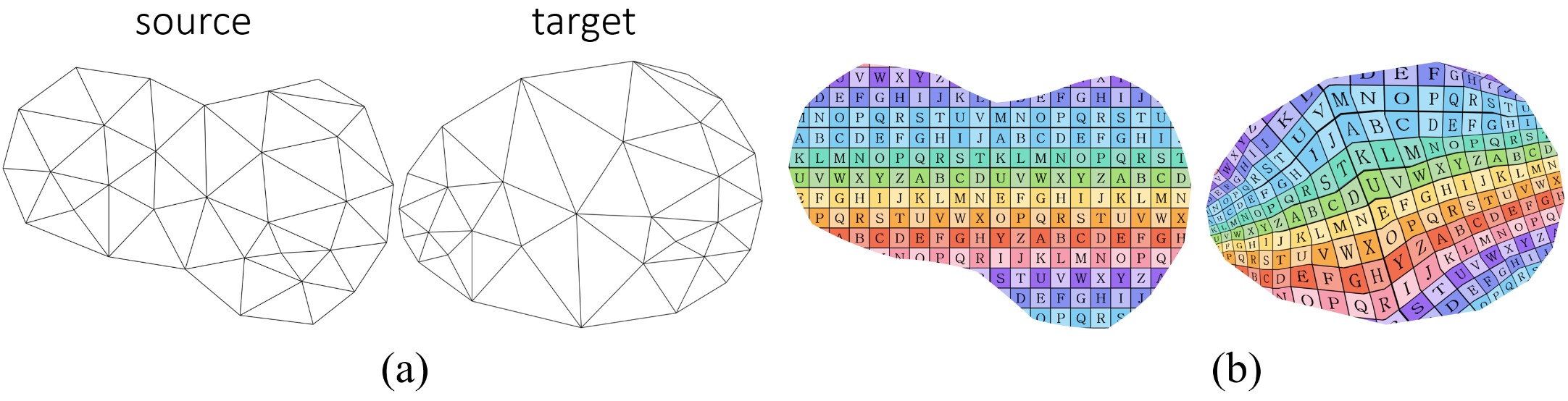
Figure 1: Piecewise-Linear map of a CETM vertex-to-vertex map [SSP08]. The input vertex to vertex map (a) and the pullback of the texture (b). Note the large angular distortion.

1.1 Related work

There is a large number of works on computing conformal maps, whether approximated, e.g., [VMW15, SC17], under some definition of discrete conformality, e.g. [SSP08], or defined smoothly on the domain e.g. [WBG09, WBGH11].

Our work, however, deals with the interpolation of a given discrete map, to a smooth map with different properties. To the best of our knowledge, there are very few such interpolators. Of course, one can use a smooth conformal [WBG09] or quasi-conformal [WBGH11] map, and add constraints for the interpolated vertices. However, such an approach will often lead to over constrained systems, which either do not interpolate the constraints, or create double covers.

In terms of local interpolators, it is possible to use a piecewise-linear map; however, it leads to visible artefacts for coarse triangulations. Furthermore, our goal is to design an interpolator that commutes with Möbius transforms, and of course, a linear (or higher order) map will in general not have this property. Finally, it is possible to use a projective interpolation scheme [SSP08, BBS17, GSC21]. This approach leads to nice results when applied to discrete conformal maps; however it is discontinuous on general deformations.

We note that some methods [CPS11, CPS15] approached conformal mappings by designing a discretized, rather than discrete (cf. [VMW15]) field of rotations and scale factors that were integrated into a map which was conformal up to integrability. Specifically, [CPS15] constructed a representation of this field in volumes that by itself construes an interpolation of Möbius maps. However, these works did not explicitly present a continuous and interpolating blend for triangle meshes as we do.

1.2 Contributions

Our main contributions are:

• BPM: A vertex-interpolating, non-linear triangle-to-triangle map, which is smooth across triangles.

• BPM is equivariant to Möbius transformations, and has low quasi-conformal distortion when the vertex-to-vertex map is discrete conformal.

• BPM provides a smooth texture pullback, even for very coarse triangulations, and for any vertex-to-vertex map.

2 Background

We describe our method first as a plane-to-plane map in global planar coordinates, and show how it is easily generalizable to curved surfaces with local intrinsic coordinates in Section 4.

2.1 Discrete and continuous maps

Consider a triangle mesh $\mathcal{M}=\left\{\mathcal{V},\mathcal{E},\mathcal{T}\right\}$, embedded in the complex plane $\mathbb{C}$ without overlaps. We parameterize the embedding by the vertex coordinates, $Z=\left\{z_{v}\in\mathbb{C}\,|\,v\in\mathcal{V}\right\}$. A map $F:Z\rightarrow W$, which transforms the vertex positions by $F(z_{v})=w_{v}$, is denoted discrete. We are mainly interested in computing an interpolation of a discrete map $F$ into a continuous map $f:\overline{Z}\rightarrow\mathbb{C}$, where $\overline{Z}$ is the union of all the triangles defined by $\mathcal{T}$ with vertex coordinates in $Z$. Such a map is interpolating when $\forall v\in\mathcal{V},\ f(z_{v})=F(z_{v})$. We define the interpolator as the operator $o:(\overline{Z},F)\rightarrow\mathbb{C}$, such that:

$$f(z)=o(z,F).$$

For instance, barycentric interpolation is an interpolator that generates piecewise-linear functions.

2.2 Holomorphic maps

A differentiable map $f\!:\!\mathbb{R}^{2}\!\to\!\mathbb{R}^{2}$, $f=(u(x,y),v(x,y))$ with a Jacobian of the form $\nabla f=\big{(}\begin{smallmatrix}a&b\\ -b&a\end{smallmatrix}\big{)}$, is holomorphic, when considered as a function on the complex plane, $f\!:\!\mathbb{C}\!\to\!\mathbb{C}$, where $f(x+iy)=u(x,y)+iv(x,y)$. Alternatively, this can be written as $\frac{\partial f}{\partial\bar{z}}=0$, indicating that a complex function that is independent of $\bar{z}$ is holomorphic. Holomorphic maps preserve the angle between any two intersecting curves, and are therefore detail preserving and useful for texture mapping. A simple example of a holomorphic map $f\!:\!\mathbb{C}\!\to\!\mathbb{C}$ is the complex affine map $f(z)=az+b$, for some $a,b\!\in\!\mathbb{C}$, which is a global similarity transformation (i.e., scale, rotation and translation). Such a map is uniquely defined by the transformation of two points.

Perhaps the quintessential holomorphic map is the Möbius transformation (defined on the extended complex plane $\hat{\mathbb{C}}=\mathbb{C}\cup{\infty}$), which has the form $m(z)=\frac{az+b}{cz+d}$, for some $a,b,c,d\!\in\!\mathbb{C}$ such that $ad-bc\neq 0$. The parameters $a,b,c,d$ are unique up to a multiplicative factor $\alpha\!\in\!\mathbb{C}$. We therefore additionally assume the normalization $ad-bc=1$, which leads to uniqueness of the parameters up to sign. By working with complex homogeneous coordinates, a Möbius transformation $m(z)$ can also be represented as a matrix $M\!=\!\big{(}\begin{smallmatrix}a&b\\ c&d\end{smallmatrix}\big{)}\!\in\!\mathbb{C}^{2\times 2}$ with determinant $1$. Then, we have $M[z;1]=[az+b;cz+d]\equiv[m(z);1]$. The matrix representation of the composition of two Möbius maps $m_{1}(m_{2}(z))$ is given by the multiplication of their matrix representations, i.e., by $M_{1}M_{2}$. Similarly, the matrix representation of $m^{-1}$ is $M^{-1}$. Möbius maps include similarities and inversions in spheres, and are defined uniquely by the transformation of three points. Since both $M$ and $-M$ represent the same transformation $m$, we use $\equiv$ to denote matrix equality up to sign, i.e. $M\equiv-M$. The choice of the sign is only required when taking a unique root or logarithm of a Möbius matrix, as elaborated in Sec. 3.2.

Barycentric blends of complex affine maps have been used successfully for generating interpolators for polygonal domains [WBGH11], by blending the complex affine maps defined by the deformation of the polygon edges. We generalize this idea, and propose to use blends of Möbius maps for generating an interpolator for a discrete map between two planar triangle meshes, by blending the Möbius maps defined by the deformation of the triangles.

2.3 Piecewise-Compatible Möbius Maps

We parameterize any discrete map $F\!:\!Z\!\to\!W$ with a set of Möbius transformations $\left\{m_{t}\,|\,t=(i,j,k)\!\in\!\mathcal{T}\right\}$ defined uniquely per triangle by the transformation of the vertices: $m_{t}(z_{i})=w_{i},m_{t}(z_{j})=w_{j},m_{t}(z_{k})=w_{k}$. We denote by $\{M_{t}\!\in\!\mathbb{C}^{2\times 2}\,|\,t\!\in\!\mathcal{T}\}$ the corresponding matrices, with components $a_{t},b_{t},c_{t},d_{t}\!\in\!\mathbb{C}$.

Compatibility condition.

A set of transformations $\left\{M_{t}\right\}$ is compatible with a map $F\!:\!Z\to W$ if the transformations of neighboring triangles agree on the map of their common vertices. Specifically, given two adjacent triangles $t_{1}=(i,j,k),t_{2}=(j,i,l)\!\in\!\mathcal{T}$ with a shared edge $e=(i,j)$, we have that $w_{i}=M_{t_{1}}(z_{i})=M_{t_{2}}(z_{i})$ and similarly for $z_{j}$.

Given a triangle mesh $\mathcal{M}$, a set of Möbius transformations $\{M_{t}\}$ that fulfills the compatibility condition defines a Piecewise-Compatible Möbius (PCM) Map  [VMW15]. It is advantageous to consider general deformations as PCMs (as opposed to, e.g., piecewise-affine maps) due to their natural connection to conformal and discrete conformal deformations. For example, PCM maps are closed under global (single) Möbius transformations. Namely, given a matrix representation $M_{g}$ of a global Möbius transformation $m_{g}$, we have that the set of transformations $\{M_{t}M_{g}\}$ and $\{M_{g}M_{t}\}$ are also PCM maps. In addition, discrete conformality (CETM) [SSP08] has an elegant description in the PCM representation in terms of the corner variables $\{X_{t,i}\!\in\!\mathbb{C}\,|\,t\!\in\!\mathcal{T},i\!\in\!t,v_{i}\!\in\!\mathcal{V}\}$, where $X_{t,i}=(c_{t}z_{i}+d_{t})^{-1}$. Specifically, a PCM map is a discrete conformal equivalence if and only if $|X_{t,i}|$ does not depend on $t$. Then, $|X_{\cdot,i}|=e^{u_{i}/2}$, where $u\!:\!\mathcal{V}\to\mathbb{R}$ is the conformal factor.

Unfortunately, unlike the piecewise-affine interpolation, the trivial interpolation of a discrete PCM map, where the Möbius transformation $M_{t}$ is applied to every point $z\in t$, is not continuous between triangles. A simple way to see this is that a Möbius map is uniquely determined by $3$ points. Therefore, the transformation of all the points on the edge shared by two triangles is compatible by both triangles if and only if they are transformed by a single Möbius transformation, which means that the entire mesh is. Our challenge is then to find an interpolator of PCM maps.

3 Blended Piecewise Möbius Maps

3.1 Blended Maps Desiderata

Given an input discrete map $F\!:\!Z\!\to\!W$, denote by $M(F)=\{M_{t}\,|\,t\in\mathcal{T}\}$ the PCM map (i.e., the Möbius matrices) induced by $F$. We define a map interpolator $o(\overline{Z},F)$ using a continuous Möbius matrix interpolator $O\!:\!(\overline{Z},M(F))\!\rightarrow\!\mathbb{C}^{2\times 2}$, namely a Möbius transformation $O(z,M(F))$ with spatially varying blended coefficients. We then define $O$ and $o$ such that:

$$[o(z,F);1]\equiv O(z,M(F))[z;1].$$ (1)

Our requirements from the PCM interpolator $O(z,M)$ of $M$ are:

1. Locality. $O(z,M)$ should depend only on the local neighborhood of $z$.

2. Identity reproduction. $O(z,\{M_{t}\equiv Id\})\equiv Id$.

3. Continuity. The resulting map $o(z,F)$ should be at least $C^{0}$-continuous between neighboring triangles.

4. Möbius equivariance. The interpolator should commute with Möbius transformations. That is, for any global Möbius transformation $M_{g}$ we have:

   $$O(z,\{M_{g}M_{t}\}) \equiv M_{g}O(z,M).$$

   $$O(z,\{M_{t}M_{g}\}) \equiv O(z,M)M_{g}.$$ (2)

   Namely, interpolating the discrete map and performing a global Möbius transformation can be done in any order for the same result.

5. Möbius reproduction. If all vertices are transformed by the same Möbius transformation $M_{g}$ then the interpolator $O$ reproduces that Möbius transformation, i.e., $O(z,M_{g})\equiv M_{g}$. This is a corollary of Properties (2) and (4).

We note that Möbius equivariance is essential for the consistency of interpolating CETM maps; the set of CETM maps are closed under Möbius transformations; specifically, any global Möbius transformation induces a CETM map. Properties (4) and (5) then guarantee that this property carries over to our interpolator.

We prove in Sec. 3.2.3 that our requirements are met by the interpolator that we define in Sec. 3.2. We further list objectives for the interpolator that we empirically witnessed in all our examples:

1. CETM interpolation. If the interpolator is applied to a CETM map $M$, then the result should be a close approximation to a continuous conformal map.

2. QC Errors are bounded. The quasiconformal error of the interpolated $M(z)$ for any $z\in t\in\mathcal{T}$ is bounded above by the (discrete) quasiconformal error of $t$ in $M$.

We list the above as objectives since we do not have explicit proofs that they are always true; nevertheless we provide ample empirical evidence in Sec. 5.

3.2 Möbius Interpolator

3.2.1 The Möbius ratio

Let $M_{t},M_{u}\in\mathbb{C}^{2\times 2}$ be two normalized Möbius matrices representing transformations on two faces adjacent at edge $e_{ij}$ (see Fig. 2). The Möbius ratio $\delta_{tu}$ is given by:

$$\delta_{tu}=M_{t}M_{u}^{-1}.$$ (3)

Intuitively, the Möbius ratio describes the difference between applying $M_{u}$ and applying $M_{t}$, in the sense that $M_{t}=\delta_{tu}M_{u}$. It is easy to check that $\delta_{tu}^{-1}\equiv\delta_{ut}$, and $\delta_{tu}\equiv Id$ if and only if $M_{t}\equiv M_{u}$. Furthermore, due to the PCM compatibility between $M_{t}$ and $M_{u}$, we have that $F(z_{i})$ and $F(z_{j})$ are fixed points of the transformation $\delta_{tu}$.

We additionally define the log Möbius ratio, given by:

$$\ell_{tu}=\log\left(\text{Sign}(\text{Tr}(\Re(\delta_{tu})))\cdot\delta_{tu}\right),$$ (4)

where $\Re()$ is the real part of a complex number, $\text{Tr}()$ is the trace operator, and $Sign()$ is the sign of a real number (outputting $\pm 1$).

Thus, $\ell_{tu}$ is the log of either $\delta_{tu}$ or $-\delta_{tu}$, whichever is closer to the identity in the Frobenius norm (see Appendix B). The square root of the Möbius ratio is correspondingly given by: $\sqrt{\delta_{tu}}=\exp(\tfrac{1}{2}\ell_{tu})$.

Boundary edges.

If $e_{ij}$ is a boundary edge, then we set its ratio to Id. That encodes the choice that the transformation “beyond” the edge is the same Möbius transformation of $t$, which naturally adheres to our requirements.

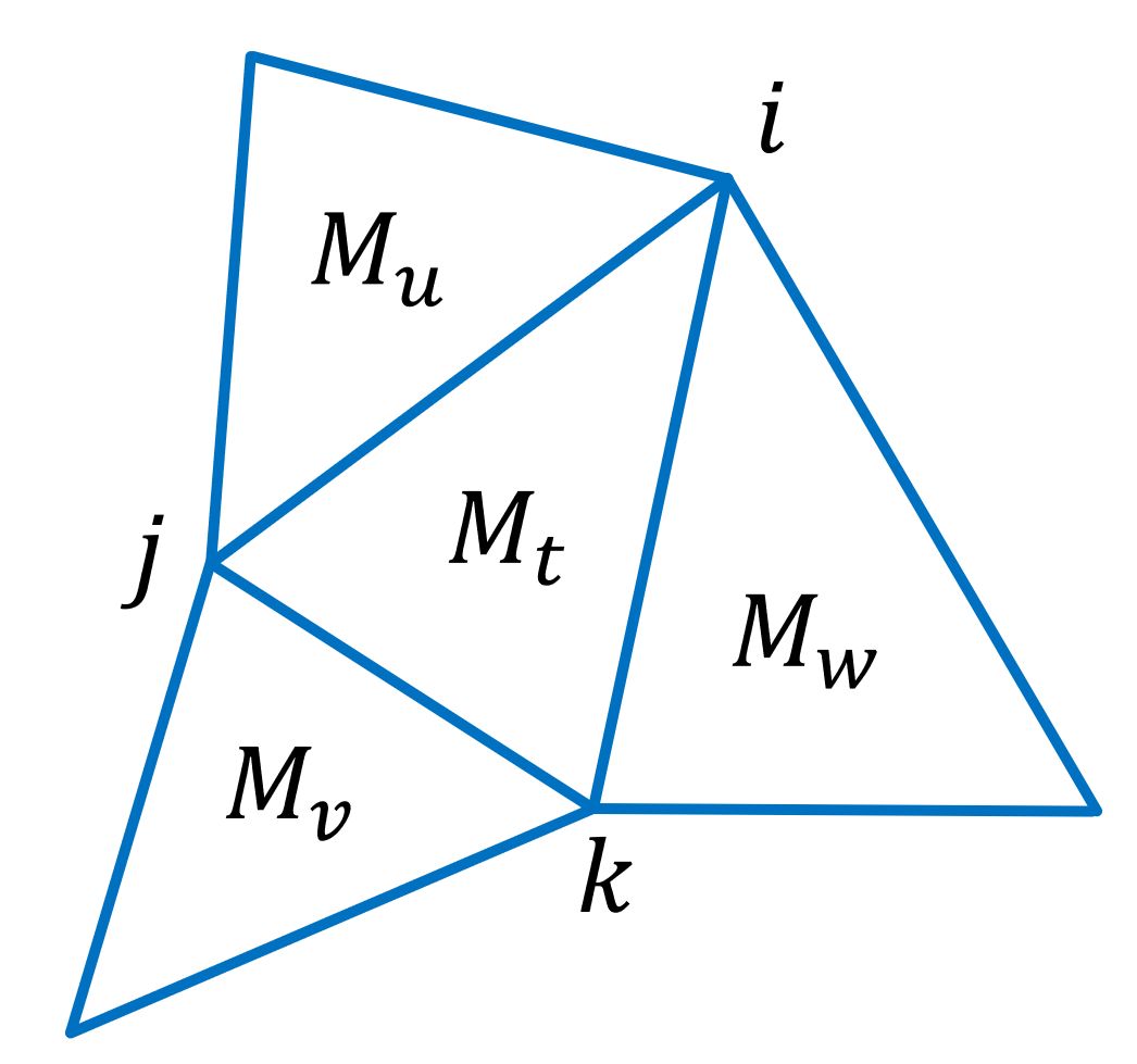
Figure 2: Our notation.

3.2.2 Ratio interpolator

Consider a face $t=ijk\!\in\!\mathcal{T}$ and neighboring triangles $u,v,w\!\in\!\mathcal{T}$ adjacent to the edges $e_{ij},e_{jk},e_{ki}\!\in\!\mathcal{E}$, respectively (Fig. 2). Each face has a corresponding Möbius matrix $M_{t},M_{u},M_{v},M_{w}$, and each edge has a corresponding log Möbius ratio of its neighboring triangles: $\ell_{ut}$, $\ell_{vt}$ and $\ell_{wt}$. We define the log ratio interpolator as:

$$\ell_{t}(z,M)=\frac{B_{ij}(z)\ell_{ut}+B_{jk}(z)\ell_{vt}+B_{ki}(z)\ell_{wt}}{B_{ij}(z)+B_{jk}(z)+B_{ki}(z)},$$ (5)

for some edge barycentric coordinates $0\leq B_{e}(z)\leq 1$, with $e\!\in\!\mathcal{E}_{t}=\{e_{ij},e_{jk},e_{ki}\}$. We require that for $e\!,\!\tilde{e}\!\in\!\mathcal{E}_{t}$, and a non-vertex point $z\!\in\!{\tilde{e}},z\!\notin\!\{z_{i},z_{j},z_{k}\}$ we have that $B_{e}(z)/\sum_{\hat{e}\in\mathcal{E}_{t}}B_{\hat{e}}(z)=1$ if $e\!=\!\tilde{e}$ and $0$ otherwise. In addition, we require that the sum of the coordinates does not vanish. Specifically, we take $B_{e}(z)={d(z,e)}^{-1}$, where $d(z,e)$ is the distance of $z$ to the line the edge $e$ lies on. See Appendix A for the implementation details.

Finally, our Möbius interpolator is given by:

$$O(z\in t,M)=\exp\left(\frac{1}{2}\ell_{t}(z,M)\right)M_{t}=\sqrt{\delta_{t}(z,M)}\,M_{t}.$$ (6)

Discussion.

Our interpolator is similar in spirit to the rotation interpolant of Alexa [Ale02], and is based on the general approach of interpolation in Lie groups [Mar99]. By linearly interpolating the log Möbius ratio, we guarantee that the blended matrix $O(z,M)$ is normalized (i.e., has determinant $1$) if the input matrices $M$ are normalized. That is because the zero-trace property is invariant under a linear blend.

3.2.3 Properties

Our interpolator is local (Req. (1)) since it is defined using a triangle and its $3$ neighbors, and it is easy to check that it reproduces the identity (Req. (2)).

Continuity on edges.

Without loss of generality, when $z\in e_{ij},z\neq z_{i},z_{j}$, we have that $\ell_{t}(z)=\ell_{ut}$ and $\ell_{u}(z)=\ell_{tu}$, and thus our interpolation reduces to:

$$O(z,M)=\sqrt{\delta_{ut}}\cdot M_{t}\equiv\sqrt{\delta_{tu}}\cdot M_{u},\quad\forall z\in e_{ij},z\neq z_{i},z_{j}$$ (7)

Hence, the Möbius interpolator on the edge $e_{ij}$ only depends on the two faces $t,u$ adjacent to the edge, and it is symmetric in $t,u$ (up to sign) leading to the same map $O(z,M)$. Note that Eq (7) is similar to SLERP interpolation for quaternions [Sho85].

Continuity on vertices.

Note that the barycentric coordinates are not continuous on a vertex (e.g. $z_{i}$), hence the ratio interpolant is also not continuous at the vertex. However, we have that $F(z_{i})$ is a fixed point of the Möbius ratios, and thus we interpolate the original PCM map at $z_{i}$. This leads to continuity on vertices across different triangles, as needed by Req. (3).

Möbius equivariance.

We first note that the ratios $\delta$ are invariant to right composition $M_{t|u|v|w}M_{g}$ with a global Möbius transformation $M_{g}$; thus, the interpolant $O$ is trivially equivariant to right composition. For left composition $M_{g}M_{t|u|v|w}$ (first PCM then global), we have a conjugated ratio $\delta_{tu}=M_{g}(M_{t}M_{u}^{-1})M_{g}^{-1}$. Since trace is invariant to cojugation, and since conjugation commutes with matrix logarithm and exponent, the entire interpolant becomes:

$$O(z\in t,\{M_{g}M_{t}\})=M_{g}\delta(z,\{M_{t}\})M_{g}^{-1}\cdot M_{g}M_{t}=M_{g}O(z\in t,M).$$ (8)

Thus, we also fulfill Req. (4), and with (2) we fulfill Req. (5).

Local injectivity.

Möbius transformations are locally injective in a region that does not contain poles. Specifically, if a single Möbius transformation $m_{t}$ of a triangle $t$ does not flip or degenerate the triangle edges, we have that $m_{t}$ has a positive Jacobian anywhere inside. Nevertheless, for the blended Möbius transformation we do not have such a guarantee. In practice, our maps are well behaved for the blending weights that we have chosen, however extreme cases may exist (see Figure 9).

4 Curved surfaces

Our method is also applicable for mapping from curved surfaces to the plane. The discrete mapping is computed locally for each triangle, by flattening it and its neighboring three triangles isometrically to the plane to generate the source triangles $Z$. The continuous mapping is then computed by blending inside the triangle, using the same scheme as in the two-dimensional case, and pulling the resulting map back to the surface.

More formally, consider a triangle mesh $\mathcal{M}=\left\{\mathcal{V},\mathcal{E},\mathcal{T}\right\}$, embedded in $\mathbb{R}^{3}$. Let $X=\big{\{}x_{v}\in\mathbb{R}^{3}\,|\,v\in\mathcal{V}\big{\}}$ be its vertex coordinates. The discrete map $F:X\rightarrow W$ transforms the vertex positions by $F(x_{v})=w_{v}\in\mathbb{C}$. We are interested in computing a continuous interpolating map $f:\overline{X}\rightarrow\mathbb{C}$, where $\overline{X}$ is the union of all the triangles defined by $\mathcal{T}$ with vertex coordinates in $\mathbb{R}^{3}$ and $\forall v\in\mathcal{V},\ f(x_{v})=F(x_{v})$.

We define for each $t\!\in\!\mathcal{T}$, a local discrete map $\tilde{F_{t}}:\tilde{Z}_{t}\rightarrow W$ where $\tilde{Z}_{t}$ is an isometric embedding in 2D of the face $t$ and its neighboring faces $u,v,w$. The corresponding Möbius matrices $M(\tilde{F_{t}})=\{M_{t},M_{u},M_{v},M_{w}\}$ are defined as before, as is the matrix interpolator $O(z,M(\tilde{F}_{t}))$, and correspondingly the interpolator $o(z,\tilde{F}_{t})$. Let $\tilde{z}_{t}\!\in\!\mathbb{C}$ be the planar point that corresponds to some point $x\in t$ on the mesh under the local isometric embedding. The interpolator is defined $\forall t\in\mathcal{T}$ as follows:

$$f_{t}(x)=f_{t}(\tilde{z}_{t})=o(\tilde{z}_{t},\tilde{F_{t}}).$$ (9)

4.1 Continuity

We need to show that this definition is well-posed, since it is defined for each triangle separately. We get this since (1) Our interpolator is Möbius equivariant, (2) there exists a Möbius map between isometric embeddings, and (3) the map of points on the edge depends only on the Möbius matrices of its neighboring triangles.

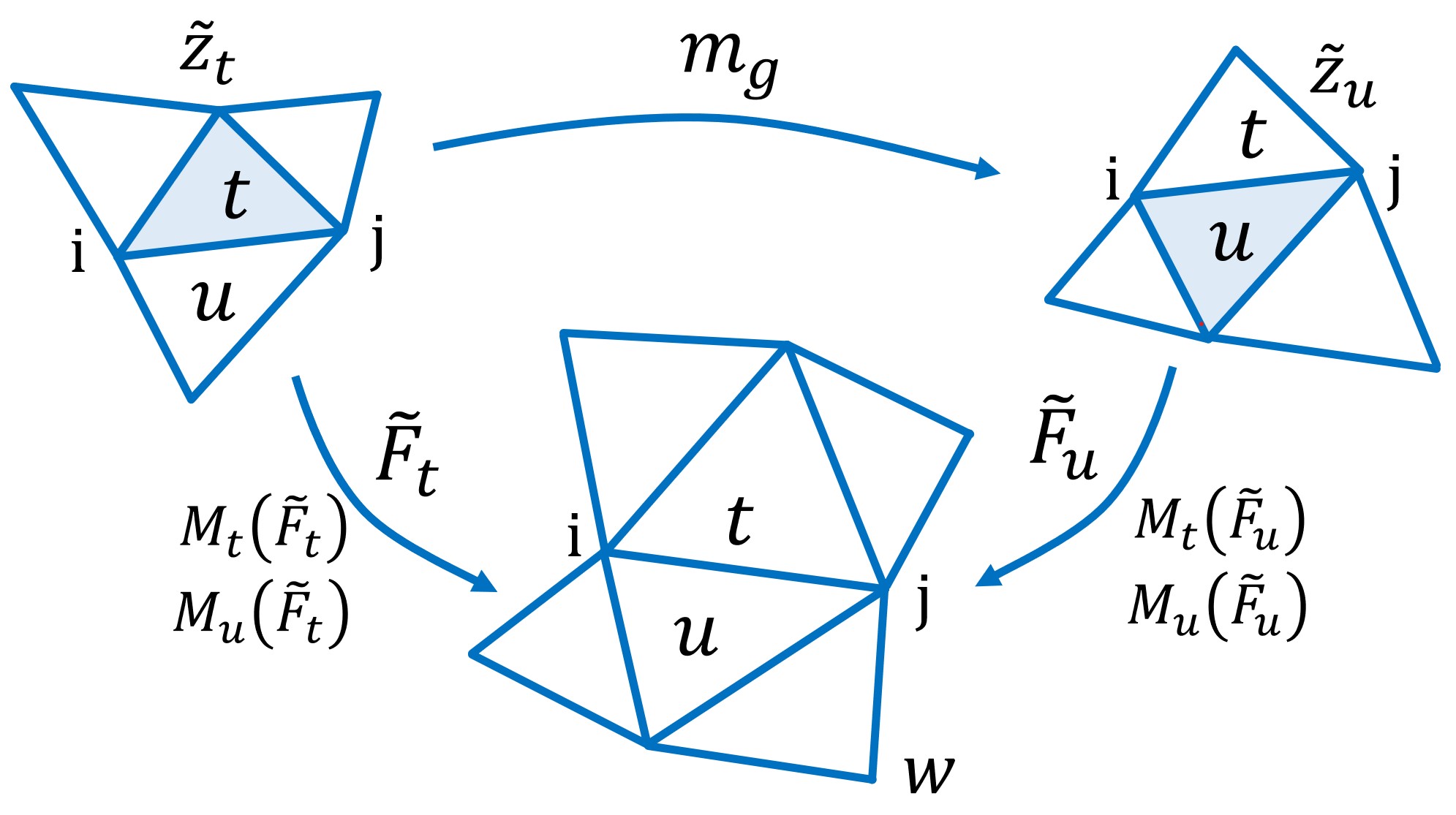
Figure 3: Notation for 3D Framework.

Formally, Let $t,u\!\in\!\mathcal{T}$, be two triangles that share an edge $e_{ij}$, and let $\tilde{Z}_{t},\tilde{Z}_{u}$ be the corresponding (independent) isometric embeddings of each triangle and its neighboring faces. See Fig. 3 for our notation. Since the two embeddings map the triangles $t,u$ isometrically to the plane, there exists a Möbius transformation $m_{g}$ such that $\forall x\!\in\!{t\cup u}$, its corresponding planar points $\tilde{z}_{t}\in\tilde{Z}_{t}$ and $\tilde{z}_{u}\in\tilde{Z}_{u}$ satisfy $\tilde{z}_{u}=m_{g}(\tilde{z}_{t})$. We denote by $M_{t}(\tilde{F}_{t}),M_{t}(\tilde{F}_{u})$ the Möbius matrices corresponding to $t$ induced by $\tilde{F}_{t},\tilde{F}_{u}$, respectively, and similarly for $M_{u}(\tilde{F}_{t}),M_{u}(\tilde{F}_{u})$. By construction, we have that:

$$M_{t}(\tilde{F}_{t})\equiv M_{t}(\tilde{F}_{u})M_{g},\quad\quad M_{u}(\tilde{F}_{t})\equiv M_{u}(\tilde{F}_{u})M_{g},$$ (10)

where $M_{g}$ is the Möbius matrix that corresponds to $m_{g}$.

Let $x\!\in\!e_{ij}$ be a point on the mutual edge of $t$ and $u$, with the corresponding planar points $\tilde{z}_{t},\tilde{z}_{u}$. The interpolator of a point on the edge depends only on the Möbius matrices of its neighboring triangles, and is given by Equation (7). We have:

$$\delta_{tu}(\tilde{F}_{t})=M_{t}(\tilde{F}_{t})M_{u}^{-1}(\tilde{F}_{t})=M_{t}(\tilde{F}_{u})M_{g}M_{g}^{-1}M_{u}^{-1}(\tilde{F}_{u})=\delta_{tu}(\tilde{F}_{u}).$$ (11)

Thus, the matrix interpolator is given by

$$O(\tilde{z}_{t},M(\tilde{F}_{t})) =\sqrt{\delta_{ut}(\tilde{F}_{t})}M_{t}(\tilde{F}_{t})=$$ (12)

$$=\sqrt{\delta_{ut}(\tilde{F}_{u})}M_{t}(\tilde{F}_{u})M_{g}=O(\tilde{z}_{u},M(\tilde{F}_{u}))M_{g}.$$

Finally, we have:

$$=O(\tilde{z}_{t},M(\tilde{F}_{t}))[\tilde{z}_{t};1]=$$ (13)

$$=O(\tilde{z}_{u},M(\tilde{F}_{u}))M_{g}M_{g}^{-1}[\tilde{z}_{u};1]=[o(\tilde{z}_{u},\tilde{F}_{u});1].$$

Hence, we have that the map interpolation is consistent, as required. Note that this consistency generalizes to any locally defined interpolator, as long as it is equivariant to maps between the local flattened patches. We present results in Fig. BPM: Blended Piecewise Möbius Maps and in Sec. 5. Note that our map is at least $C^{0}$ continuous, but not $C^{1}$ in general.

We provide the pseudo code for our algorithm in Appendix C.

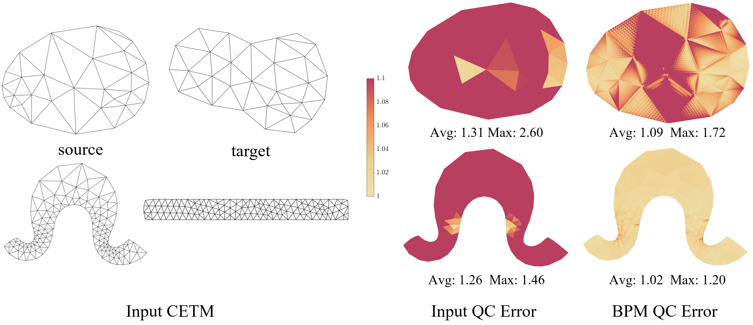
Figure 4: CETM as input. (left) The input CETM deformation. (right) The QC errors of the input discrete deformation and the BPM mapping. Note that the error of BPM is considerably lower than the input errors.

5 Experimental Results

We use a variety of examples to demonstrate the effectiveness of our interpolators. For each example, we show the source and target meshes, and visualize the map by (1) pulling back a texture from the target mesh to the source mesh, as well as (2) pushing forward a texture from the source mesh to the target mesh. Note that on the target mesh, the edges are curved. While our interpolator is smooth and in closed-form, computing the resulting Quasi-conformal (QC) distortion introduces a complicated expression which varies non-linearly within the triangle. To facilitate its visualization, we simply approximate the resulting QC error by refining the source mesh using $4$ levels of subdivision, applying the computed (continuous, non-linear) interpolator to the refined vertices, and computing the QC distortion of the linear map between the subdivided triangles. For a single subdivided triangle, the QC distortion is given by the ratio of the singular values of the linear map [SSGH01].

For the input discrete deformations we use different deformations/parameterization techniques. We use Conformal Equivalence of Triangle Meshes (CETM)  [SSP08] and Boundary-First Flattening (BFF) [SC17] for generating discrete conformal input maps. For pure planar deformations, we use As-Möbius-as-possible (AMAP) [VMW15] for discrete maps with small QC and CETM distortion. We use Cauchy coordinates (CC) [WBG09] to generate discrete deformations sampled from continuous conformal maps. We additionally use As-Killing-As-Possible shape deformation (AKVF)  [SBBG11] to generate inputs that are far from conformal. For additional mappings of surfaces to the plane we use models from the recent parameterization dataset [SSS22] in Figs. 15, 17. The parameterization method used is mentioned in each example.

For comparison, we consider piecewise linear (PL) interpolation, and circumcircle preserving projective interpolation (PROJ) [SSP08, BBS17].

5.1 Properties

We first validate the two objectives mentioned in Sec. 3.1.

CETM as input.

When the discrete input map is a conformal equivalence, i.e., fulfills the CETM conditions, our interpolator leads to a low QC distortion, even when the QC distortion of the input map is quite large. We demonstrate this for two input deformations in Fig. 4.

Bounded QC Errors.

In all cases the QC error of our map is lower than the QC error of the input map. When the input deformation is close to conformal (Figs. 10, 11, 14), our method gives the best results. However, even for deformations far from conformal, (Fig. 12), our mapping is smooth with small QC errors.

5.2 Robustness

We demonstrate the robustness of our approach to different meshes.

Non-uniform triangulations.

We use a mesh whose left and right halves are meshed differently. We deform it using AKVF, and show the interpolation results in Fig. 5. Note that the texture deformed using our map looks similar on the left and right side of the mesh, thus our method is not sensitive to meshing.

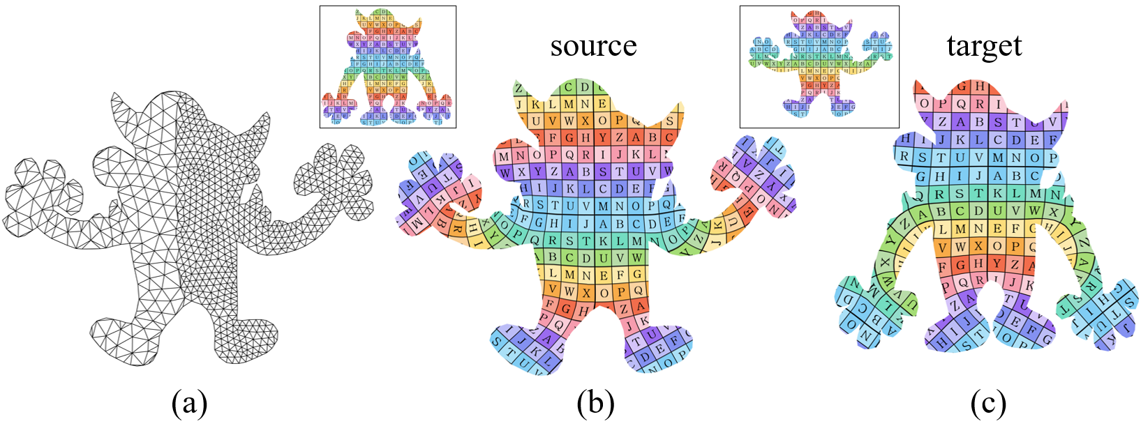
Figure 5: Non-uniform triangulations. (a) The input triangulation, (b) the pullback and (c) push-forward of the texture shown in a black frame with our mapping.

Non simply connected.

Our method is applicable to meshes of any topology. We demonstrate it on a few non-simply connected meshes in Fig. 6.

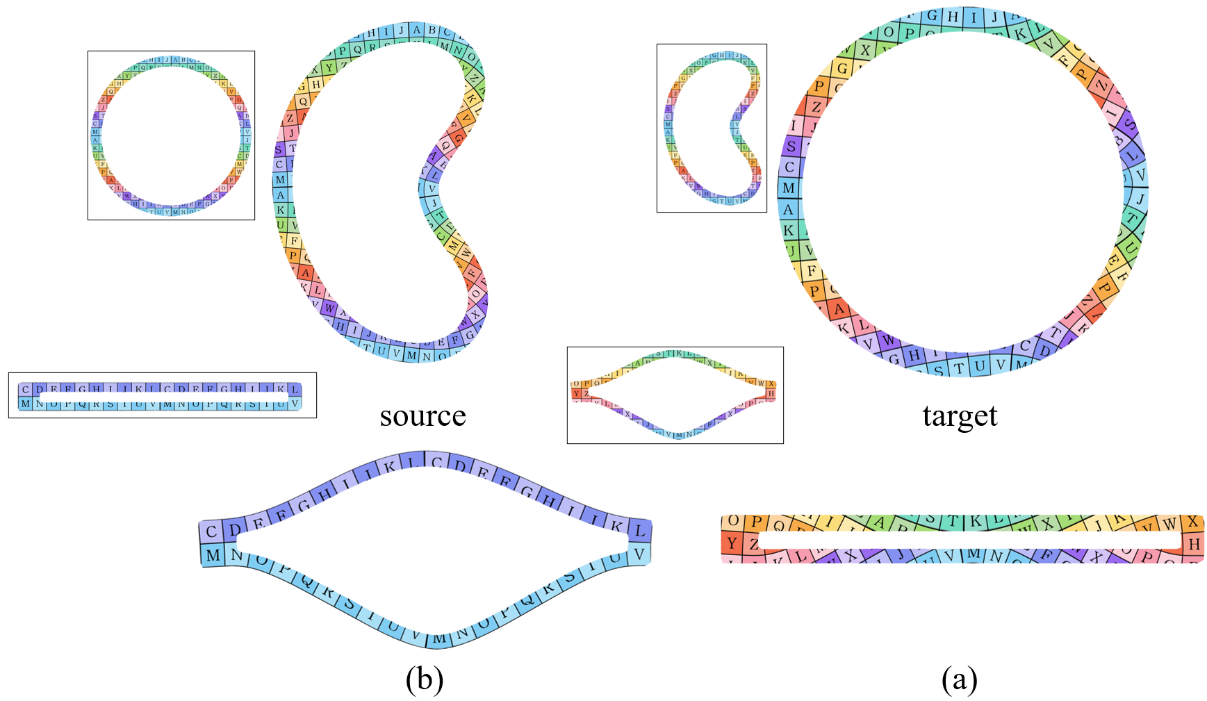
Figure 6: Non simply connected meshes. (a) The pull-back, and (b) the push-forward of the texture (shown in a black frame) using our mapping for two non simply connected meshes.

Different resolutions.

We remesh a model to $4$ different resolutions, and apply the same deformation by sampling the continuous Cauchy Coordinates, using the same source and target cages. We show the result in Fig. 7, and compare with piecewise-linear interpolation. Note that, unlike the PL map, our results are virtually indistinguishable across resolutions, despite the very different mesh resolutions.

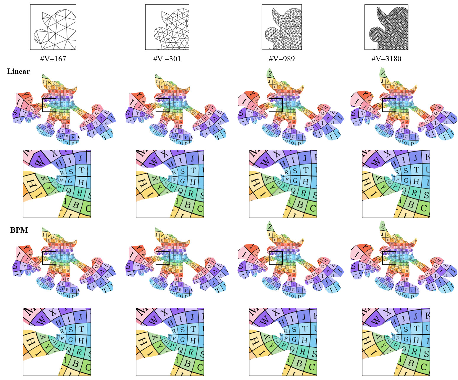
Figure 7: Multiple resolutions. Pull-back of our mapping. from left to right: increased mesh density. Note that our mapping of the coarse triangulation (bottom left) is comparable to the linear map on the much denser triangulation (top right).

Large deformations.

We assume that the discrete map is slowly varying between triangles, therefore $\delta_{tu}$ is close to $Id$ or $-Id$, and the chosen logarithm branch will be the same for the $3$ edges of the triangle. However, even if this is not the case, our interpolator is smooth, but may be more oscillatory. In this experiment, we demonstrate that our map is resilient to large changes in the deformation of neighboring triangles. In Fig. 8 we show a discrete map with very large deformations, where our map is still smooth.

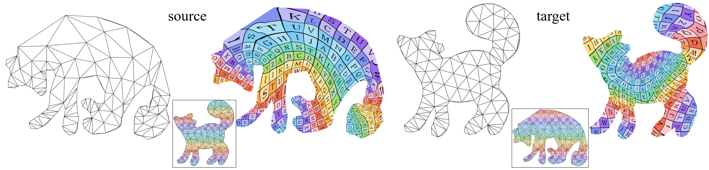
Figure 8: Even when the input map is far from conformal (here computed using AKVF), our interpolator leads to a smooth map.

Local injectivity

as mentioned in Sec. 3.2, our interpolator is not formally guaranteed to be locally injective. In fact, as we demonstrate in Fig. 9, this might be the case even if the deformed triangles are not flipped. This happens when the ratios $\delta$ are very different between the edges of the same triangle, which eventually results from a big variation in the Möbius transformation between neighboring triangles. Since parameterization algorithms try to avoid such variations with regularization, we do not expect this to occur often in practice.

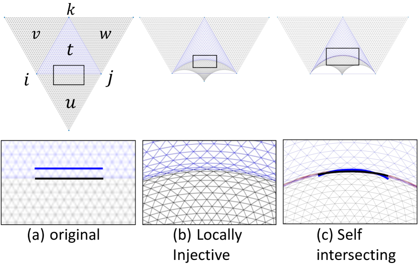
Figure 9: Example of a non-locally-injective transformation. (a): original triangles with part of $e_{ij}$ in black and a parallel line inside $t$ in blue. (b): an extreme deformation with matrix $M$ of the bottom triangle $u$ (while the rest are stationary) leads to edge ratios $\delta_{ut}=M,\delta_{vt}=\delta_{wt}=Id$. However, the result is still locally injective. By the barycentric blending, any line originally parallel to $e_{ij}$ in $t$ is transformed by matrices $M^{d}$, with varying $d<\frac{1}{2}$, and thus closer to $Id$ than the transformation $M^{\frac{1}{2}}$ of $e_{ij}$. In this case, $e_{ij}$ would be more curved inwards than the other parallel lines within. Thus, in (c), when $M$ is made even more extreme, the target black circular arc from edge $e_{ij}$ and the less-curved blue curve transformed by $M^{d}$ intersect, causing a loss of injectivity.

5.3 Comparisons

Interpolators on triangles.

We compare our approach to PL and projective interpolation, for inputs created with a variety of deformation methods (AMAP, CETM, BFF, AKVF, CC). The projective interpolation requires the computation of scaling factors per vertex, which we compute individually per triangle. Note that for meshes that are not CETM, the scaling factors do not agree between different triangles sharing vertices, and therefore the interpolation can be discontinuous. We show in Figs. 10, 11, 14, 12 the resulting texture maps, as well as the QC distortion for each example. Note that for discrete conformal maps (CETM), and for maps that are close to conformal (BFF, PCM), both the projective interpolation and our approach achieve a good result, though our QC error is lower. Furthermore, our method is applicable to any discrete map, whereas projective interpolation is discontinuous for non-CETM maps. This is clearly visible for meshes deformed using AKVF, which can induce significant angle distortion (see Fig. 12). Compared to PL interpolation, our map is smoother even for very coarse triangulations (see also Fig. 7).

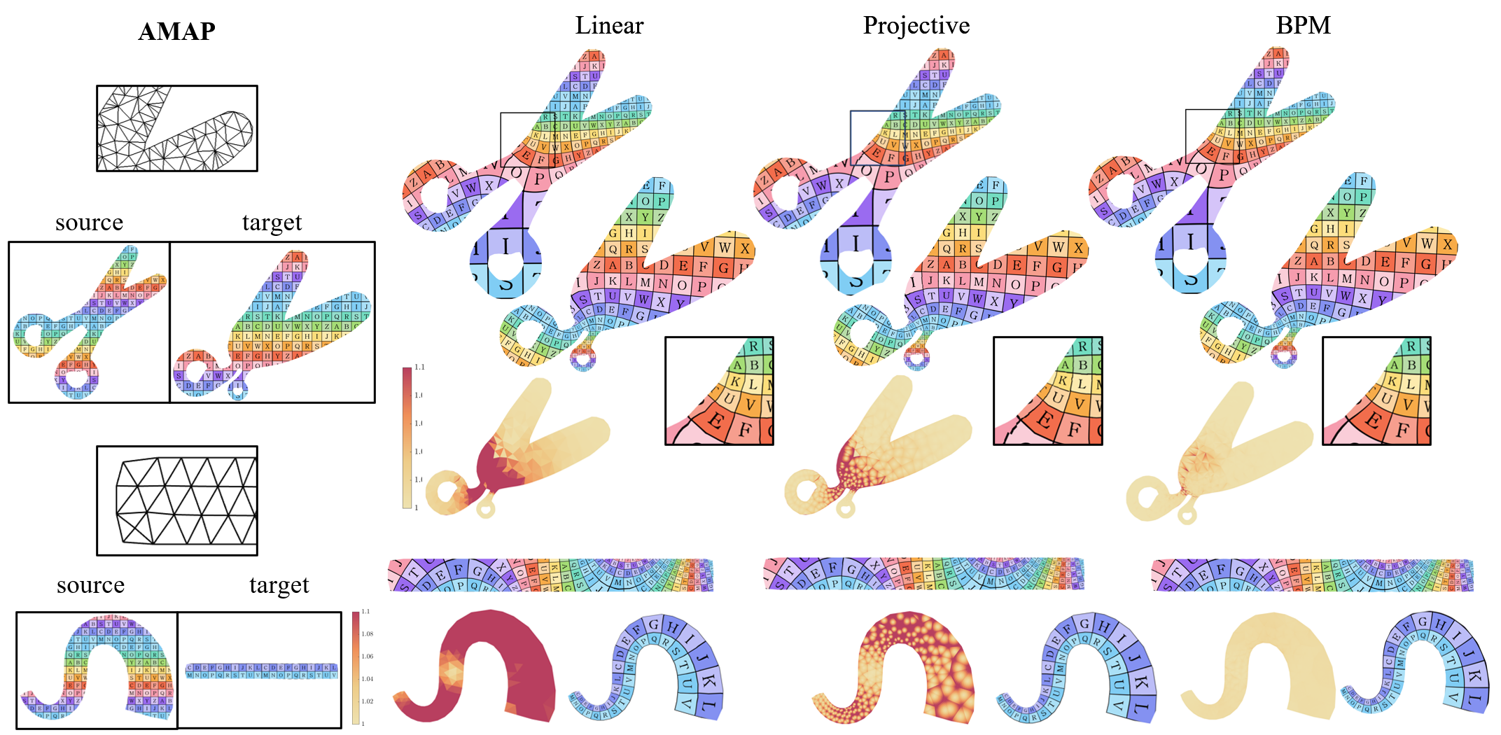
Figure 10: We compare BPM to linear and projective maps for planar meshes, on input deformations computed using the AMAP method. Note the artefacts in the linear map, and the discontinuities in the projective map, highlighted in the zoomed images. Further, note that our approach yields lower quasi-conformal distortion compared to the alternatives.

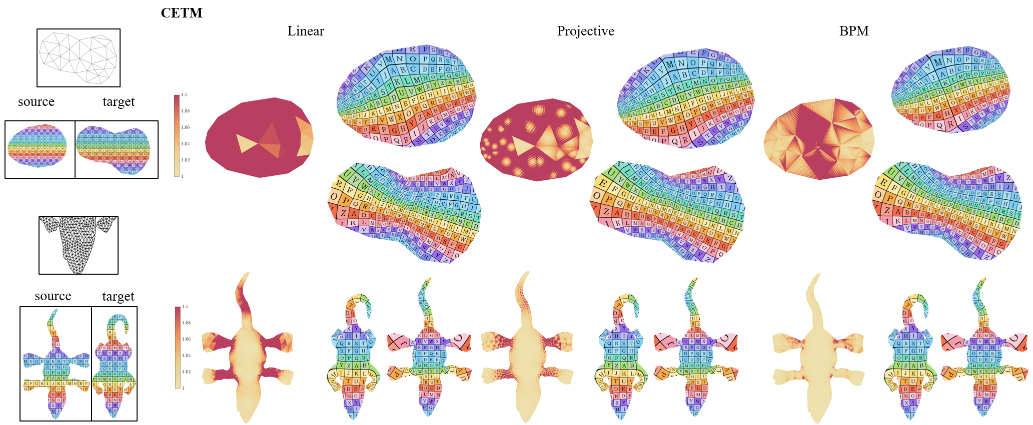
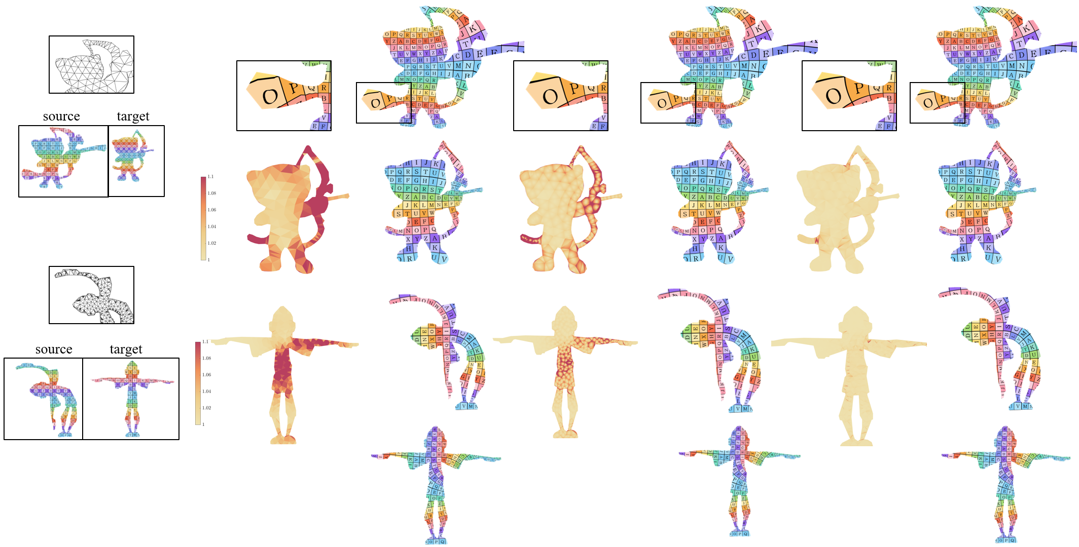
Figure 11: We compare BPM to linear and projective maps, on two planar shapes which are conformally equivalent (CETM). On this data, our interpolator is comparable to the projective approach, leading to similar texture transfers but lower QC errors.

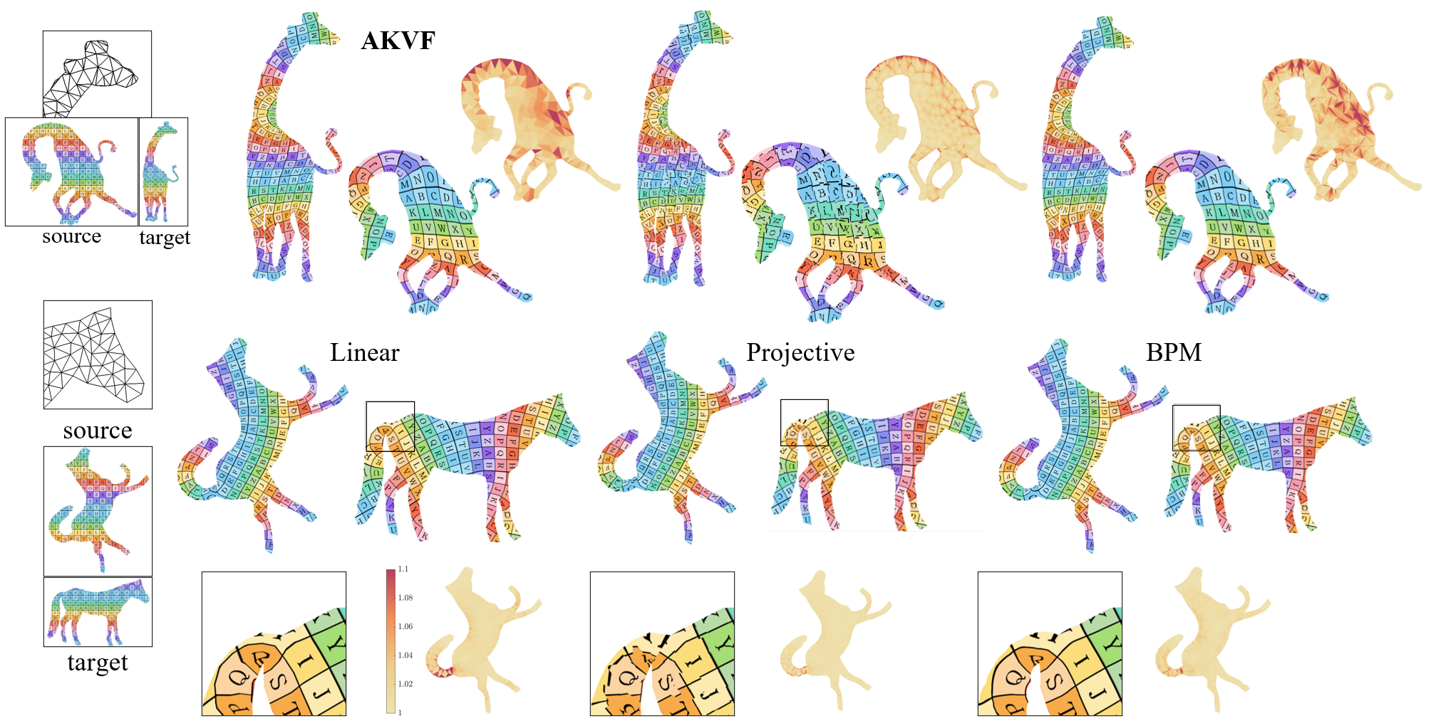
Figure 12: We compare BPM to linear and projective maps, on planar planar input computed using AKVF. Here, the maps are strongly non-conformal, leading to visible discontinuities in the projective map, whereas our approach leads to smooth results.

Continuous interpolators.

Instead of interpolating each triangle separately, or by blending, we attempt to use a continuous interpolator with constraints. Namely, we use a method for which the map is given on the full source triangulation domain (and not only on the vertices), and constrain the vertices to the locations prescribed by the discrete input map. We use Cauchy Coordinates as a smooth interpolator, as it is exactly holomorphic. Fig. 13 shows the result of the comparison. On a coarse mesh, if we use a small number of vertices for the cage, the constraints on the vertices cannot be achieved. If, on the other hand, we use a large number of cage vertices, the map generates poles and overlaps. Furthermore, deformation with Cauchy Coordinates is only feasible for a mesh with a small number of vertices, as it is a global approach, that requires solving a linear system with a dense matrix. Hence, our local closed-form approach is a better alternative.

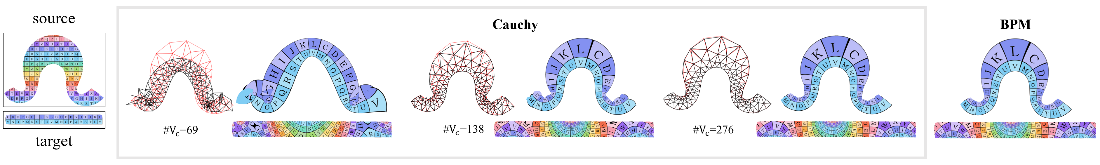
Figure 13: We compare our approach to computing a smooth map using Cauchy Coordinates, with the input vertex map as constraints and $V_{C}$ cage vertices. Note that the result highly depends on the number of cage vertices. Using a number that is too small (Cauchy, left), there are not enough degrees of freedom to reproduce the constraints and the mapping becomes a double cover. Using too many cage vertices (Cauchy, center, right) leads to visible oscillations near the boundary. Our approach (right) leads to a smooth interpolation, which is non-oscillatory, does not require additional degrees of freedom, and is closed-form.

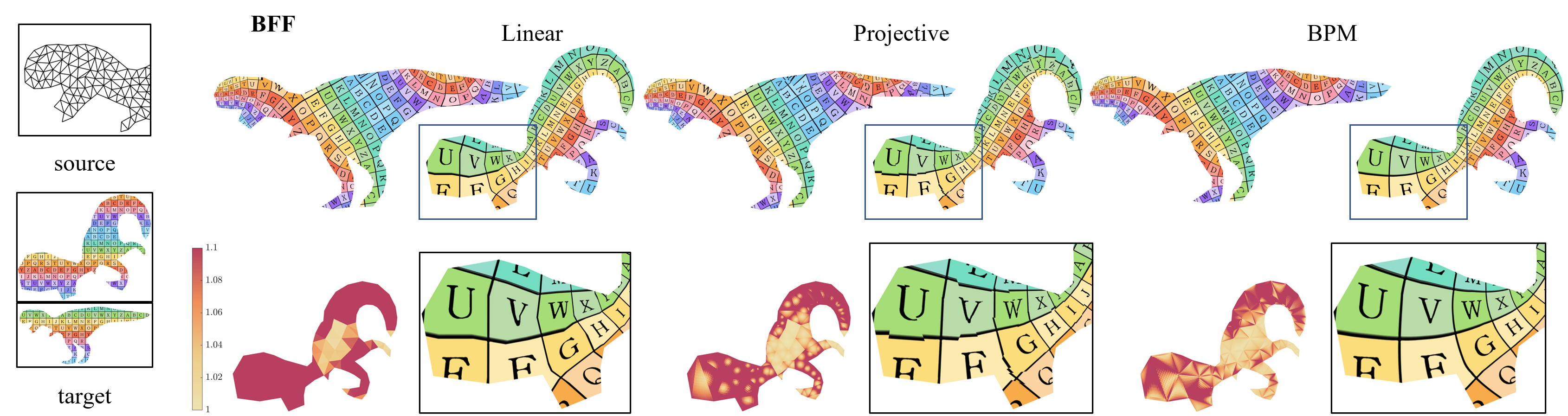
Figure 14: We compare BPM to linear and projective maps, on input computed using BFF. Here, our approach achieves similar QC distortion as the projective approach. However, since the map is not exactly discrete conformal, the projective map leads to discontinuities.

5.4 Application to texture mapping

Using the intrinsic formulation presented in Sec. 4 we interpolate the texture coordinates of 3D meshes, leading to considerably smoother textures compared to the alternatives (PL and projective). We demonstrate this in Figs. 15, 16, 17, where the inputs are generated using CETM, BFF, and designed by artists, respectively. For CETM, the results are comparable to the projective interpolation, yet our approach achieves lower QC errors, and somewhat smoother outputs. For BFF and artists’ generated parameterizations, the projective interpolation is discontinuous, and our results are considerably smoother than both the linear and projective approaches.

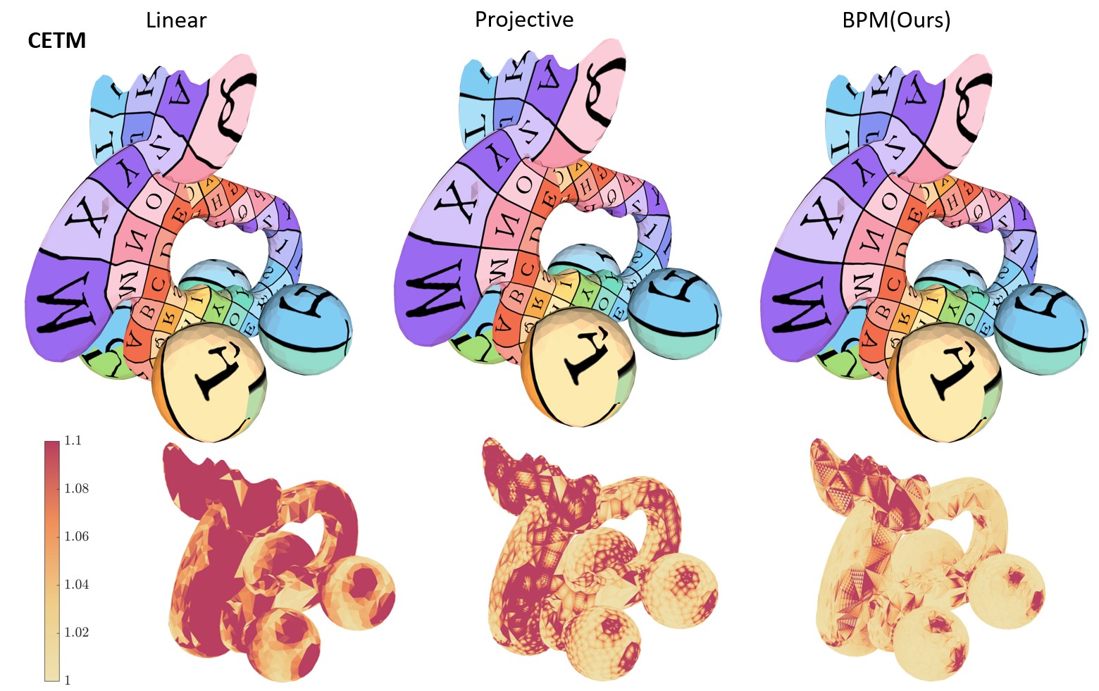
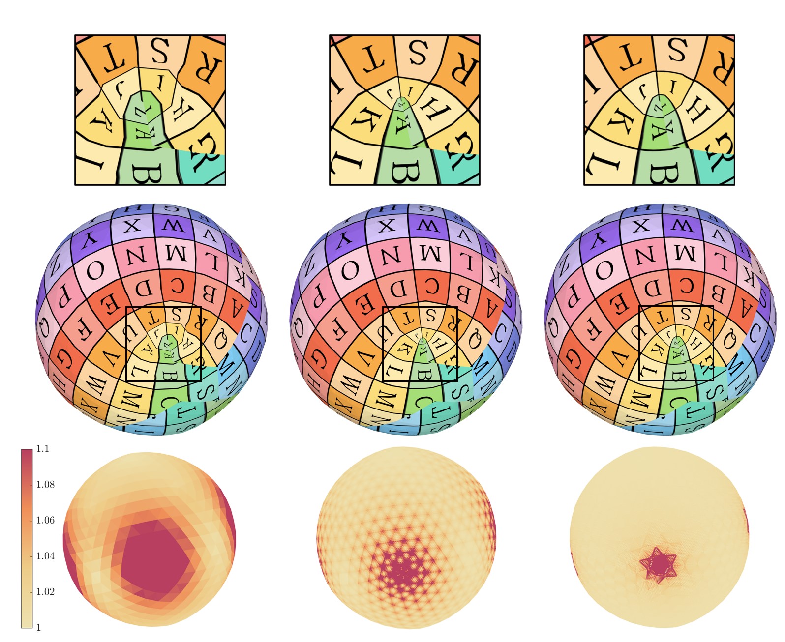
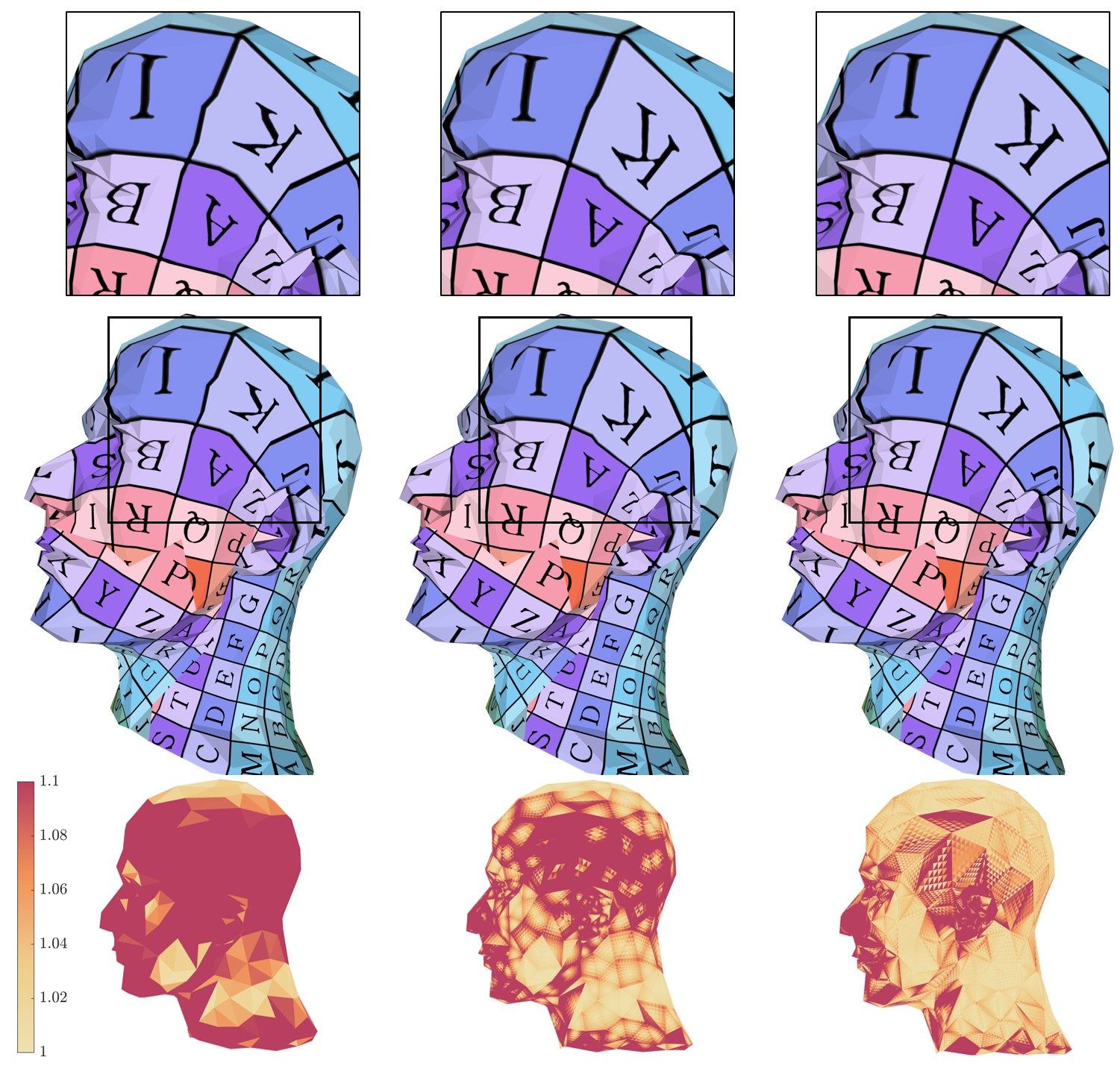
Figure 15: Applying BPM for interpolating texture coordinates generated using CETM. Projective interpolation is comparable to BPM for CETM inputs, although it generates more artifacts and QC errors.

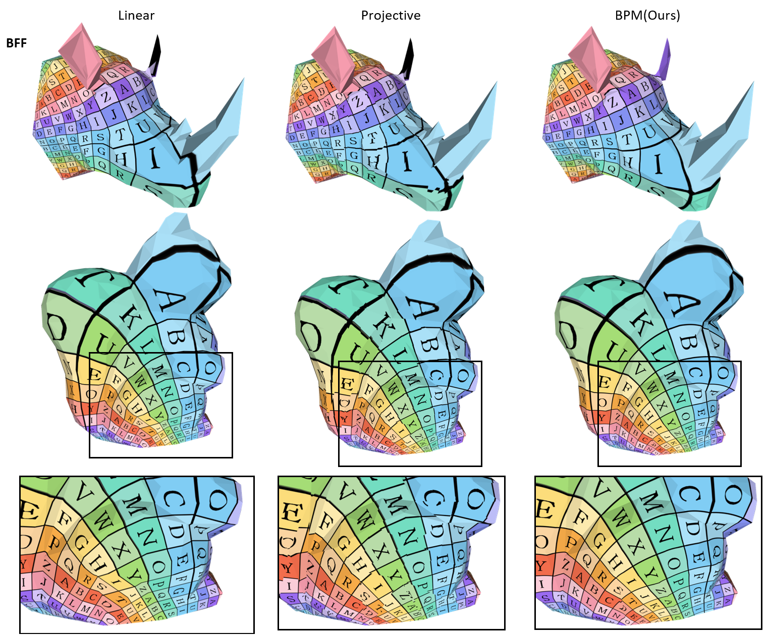
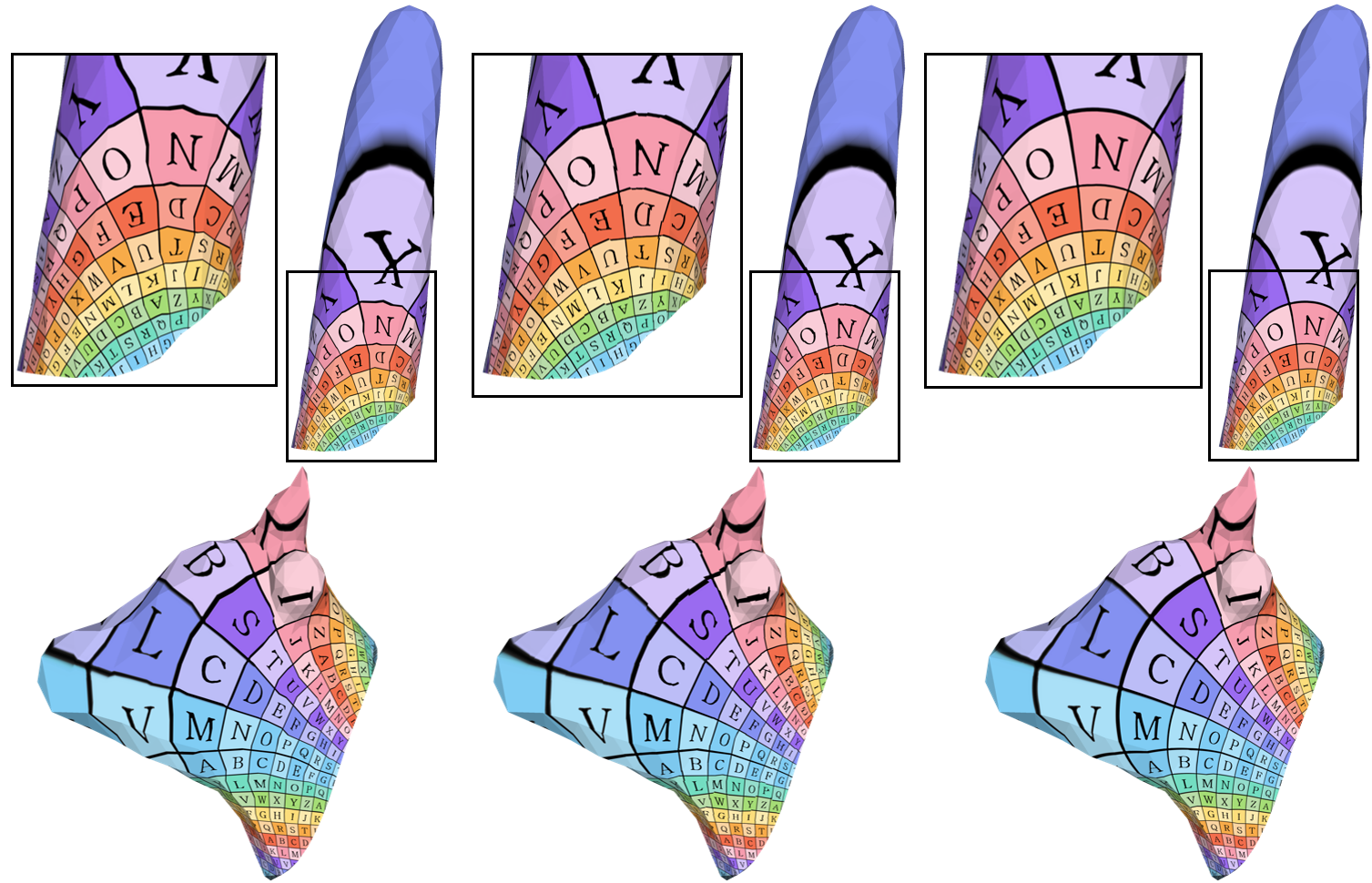
Figure 16: Applying BPM for interpolating texture coordinates generated using BFF. Note the considerably smoother texture achieved by our approach, compared to piecewise-linear and projective interpolations.

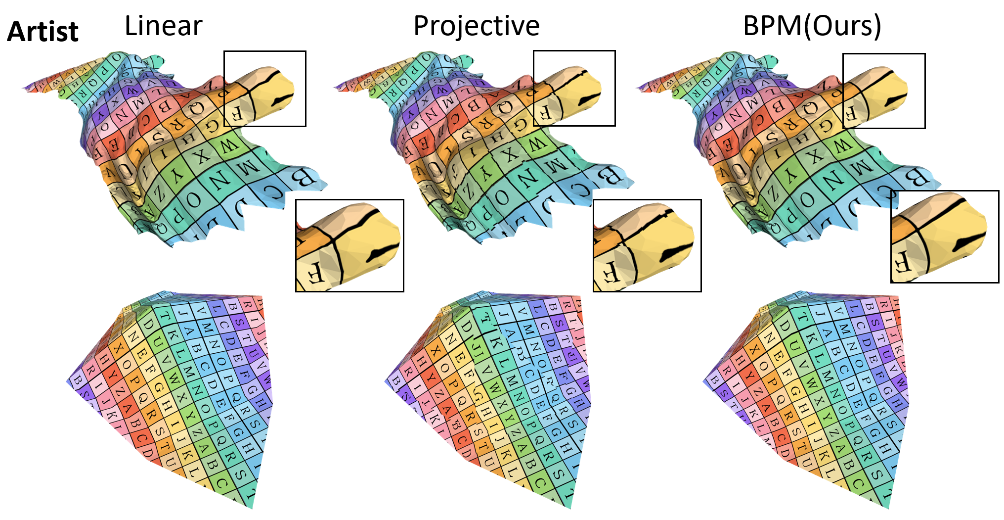
Figure 17: Interpolation for the artist-UV models from the data-set in  [SSS22]. The projective interpolation is discontinuous and generates artifacts.

6 Conclusion and Future Work

We presented a blending scheme (BPM) of Möbius transformations that interpolates a discrete map between triangulations to a continuous map on the input domain. Our scheme leads to small quasi-conformal errors when the input discrete map is close to conformal, and is applicable to any discrete input map. We additionally showed that our blending scheme can be done intrinsically, thus allowing non-linear interpolation of the texture coordinates of a 3D mesh. In the future we plan to explore other applications for our interpolation scheme, such as surface to surface, spherical parameterization, etc. In addition, we plan to investigate time interpolation in this setting, as well as generalizing our scheme to blends where the input map is approximated instead of interpolated. Finally, we aim to derive theoretical bounds for the QC error of our blends, and classify the conditions under which the map is provably bijective.

7 Acknowledgments

Mirela Ben-Chen acknowledges the support of the Israel Science Foundation (grant No. 1073/21).

.1 Appendix A: Limits of edge barycentric coordinates

The edge weights $B_{e}(z)$ that we use in Equation (5) are given in terms of the inverse distance to the edge $d(z,e)^{-1}$, which diverges as $z$ approaches the edge. However, the normalized barycentric coordinates:

$$\gamma_{e}(z)=\frac{B_{e}(z)}{B_{ij}(z)+B_{jk}(z)+B_{ki}(z)}$$ (14)

have a well-defined limit as $z$ approaches the edge (but not the vertices). To avoid reaching infinity on the edge, a simple calculation shows that the coordinates can be computed using only the distances $r_{e}(z)=d(e,z)$:

$$\gamma_{ij}(z) =\frac{r_{jk}(z)r_{ki}(z)}{s(z)},\quad\gamma_{jk}(z)=\frac{r_{ij}(z)r_{ki}(z)}{s(z)},\quad\gamma_{ki}(z)=\frac{r_{ij}(z)r_{jk}(z)}{s(z)},$$ (15)

$$s(z) =r_{jk}(z)r_{ki}(z)+r_{ij}(z)r_{jk}(z)+r_{ij}(z)r_{ki}(z)$$

It is easy to check that if only one of the $r$ quantities goes to 0, i.e., $z$ approaches an edge but not a vertex, the coordinates behave as required, i.e., equal to $1$ on the corresponding edge, and to $0$ on the other two. However, when $z$ approaches a vertex, the coordinates are still undefined. Note that in our scheme the vertices are interpolated by definition, and therefore we do not need to use the coordinates to map the original vertices. In practice, we use an epsilon value on the order of machine precision to check if the mapped point corresponds to an input vertex. We have not encountered any numerical instabilities with this approach.

.2 Appendix B: Proof for equation (4)

We minimize $\lVert\delta-I\rVert_{F}^{2}$ where $\delta\in\{-\delta_{tu},\delta_{tu}\}$, in terms of the Frobenius norm:

$$\lVert\delta-I\rVert_{F}^{2}= \text{Tr}((\delta-I)^{*}(\delta-I))=$$ (16)

$$tr(\delta^{*}\delta)-tr(\delta^{*}+\delta)+tr(I) =$$

$$tr(\delta^{*}\delta)-tr(2\Re(\delta))+tr(I).$$

This term is minimized for $max(tr(2\Re(\delta)))$, and thus $\ell_{tu}=log\left(\text{Sign}(\text{Tr}(\Re(\delta_{tu})))\delta_{tu}\right)$.

.3 Appendix C: Pseudo Code

We give a pseudo-code description of our interpolator, where Alg. 2 computes the planar-to-planar interpolation, and Alg. 3 computes the curved-surface interpolation (Sec. 4).

ApplyMoebius $(z,M)$

       inputs :  A point $z\!\in\!\mathbb{C}$, a Möbius matrix M $\!\in\!\mathbb{C}^{2\times 2}$

       output : $w\in\mathbb{C}$

       $\begin{bmatrix}w_{1}\\ w_{2}\end{bmatrix}$ = M$\begin{bmatrix}z\\ 1\end{bmatrix}$

       $w=\frac{w_{1}}{w_{2}}$

      return w 

ALGORITHM 1 ApplyMoebius

BPM $(F)$

       inputs :  A discrete map $F\!:\!Z\!\to\!W$

       output : a continuous map $f:\overline{Z}\rightarrow\mathbb{C}$

       Compute the PCM map $M(F)$ (Sec. 2.3)

       foreach $t\!\in\!\mathcal{T}$ do

            foreach $z\in t$ do

                  $u,v,w$ = neighboring triangles of $t$

                   $M_{z}=MoebiusInterpolator(z,Z,M_{t},M_{u},M_{v},M_{w})$ $f(z)=ApplyMoebius(z,M_{z})$

             end foreach

            

       end foreach

      return $f$ 

ALGORITHM 2 BPM

BPMCurved $(F)$

       inputs :  A discrete map $F\!:\!X\!\to\!W$

       output : a continuous map $f:\overline{X}\rightarrow\mathbb{C}$

       foreach $t\!\in\!\mathcal{T}$ do

            Compute discrete isometric embedding $\tilde{Z}_{t}$ (Sec. 4)

             Compute discrete map $\tilde{F_{t}}:\tilde{Z}_{t}\rightarrow W$

             Compute the PCM map $M(\tilde{F}_{t})$ (Sec. 2.3)

             foreach $x\in t$ do

                  $z=\tilde{Z}_{t}(x)$ (embed $x$)

                   $O(z,M(\tilde{F}_{t}))=MoebiusInterpolator(z,\tilde{Z}_{t},M_{t},M_{u},M_{v},M_{w})$

                   $f(z)=ApplyMoebius(z,O(z,M(\tilde{F}_{t})))$

             end foreach

            

       end foreach

      return $f$ 

ALGORITHM 3 BPMCurved

MoebiusInterpolator $z,Z_{t},M_{t},M_{u},M_{v},M_{w}$

       inputs :  A point $z\!\in\!\mathbb{C}$ ,$Z_{t}$, The embedding of triangle $t=ijk$ and its neighbors $u,v,w$ (Fig. 2), $M_{t},M_{u},M_{v},M_{w}\!\in\!\mathbb{C}^{2\times 2}$ the Möbius matrices

       output : $M_{z}$ the Möbius matrix interpolator at $z$

       /* Möbius ratios (Eq. (3)) */

       $\delta_{ut}=M_{u}M_{t}^{-1}$, $\delta_{vt}=M_{v}M_{t}^{-1}$, $\delta_{wt}=M_{w}M_{t}^{-1}$

       /* log Möbius ratios (Eq. (4)) */

       $\ell_{ut}=\log\left(\text{Sign}(\text{Tr}(\Re(\delta_{ut})))\cdot\delta_{ut}\right)$

       $\ell_{vt}=\log\left(\text{Sign}(\text{Tr}(\Re(\delta_{vt})))\cdot\delta_{vt}\right)$

       $\ell_{wt}=\log\left(\text{Sign}(\text{Tr}(\Re(\delta_{wt})))\cdot\delta_{wt}\right)$

       /* Barycentric coord. (Eq. (15)) */

       $s(z)=r_{jk}(z)r_{ki}(z)+r_{ij}(z)r_{jk}(z)+r_{ij}(z)r_{ki}(z)$ $\gamma_{ij}(z)=\frac{r_{jk}(z)r_{ki}(z)}{s(z)}$ $\gamma_{jk}(z)=\frac{r_{ij}(z)r_{ki}(z)}{s(z)}$ $\gamma_{ki}(z)=\frac{r_{ij}(z)r_{jk}(z)}{s(z)}$

       /* Blended log ratio (Eq.(5)) */

       $\ell_{t}(z,M)=\gamma_{ij}(z)\ell_{ut}+\gamma_{jk}(z)\ell_{vt}+\gamma_{ki}(z)\ell_{wt}$

       /* Möbius interpolator (Eq. (6)) */

       $M_{z}=\exp\left(\frac{1}{2}\ell_{t}(z,M)\right)M_{t}$

       return $M_{z}$

ALGORITHM 4 MoebiusInterpolator

References

- [Ale02] Marc Alexa “Linear combination of transformations” In ACM Transactions on Graphics (TOG) 21.3 ACM New York, NY, USA, 2002, pp. 380–387
- [BBS17] Stefan Born, Ulrike Bücking and Boris Springborn “Quasiconformal dilatation of projective transformations and discrete conformal maps” In Discrete & Computational Geometry 57.2 Springer, 2017, pp. 305–317
- [CPS11] Keenan Crane, Ulrich Pinkall and Peter Schröder “Spin Transformations of Discrete Surfaces” In ACM Trans. Graph. 30 New York, NY, USA: ACM, 2011
- [CPS15] Albert Chern, Ulrich Pinkall and Peter Schröder “Close-to-conformal deformations of volumes” In ACM Transactions on Graphics (TOG) 34.4 ACM New York, NY, USA, 2015, pp. 1–13
- [GSC21] Mark Gillespie, Boris Springborn and Keenan Crane “Discrete Conformal Equivalence of Polyhedral Surfaces” In ACM Trans. Graph. 40.4 New York, NY, USA: ACM, 2021
- [Mar99] Arne Marthinsen “Interpolation in Lie groups” In SIAM Journal on Numerical Analysis 37.1 SIAM, 1999, pp. 269–285
- [SBBG11] Justin Solomon, Mirela Ben-Chen, Adrian Butscher and Leonidas Guibas “As-killing-as-possible vector fields for planar deformation” In Computer Graphics Forum 30.5, 2011, pp. 1543–1552 Wiley Online Library
- [SC17] Rohan Sawhney and Keenan Crane “Boundary first flattening” In ACM Transactions on Graphics (ToG) 37.1 ACM New York, NY, USA, 2017, pp. 1–14
- [Sho85] Ken Shoemake “Animating rotation with quaternion curves” In Proceedings of the 12th annual conference on Computer graphics and interactive techniques, 1985, pp. 245–254
- [SSGH01] Pedro V Sander, John Snyder, Steven J Gortler and Hugues Hoppe “Texture mapping progressive meshes” In Proceedings of the 28th annual conference on Computer graphics and interactive techniques, 2001, pp. 409–416
- [SSP08] Boris Springborn, Peter Schröder and Ulrich Pinkall “Conformal equivalence of triangle meshes” In ACM SIGGRAPH 2008 papers, 2008, pp. 1–11
- [SSS22] Georgia Shay, Justin Solomon and Oded Stein “A Dataset and Benchmark for Mesh Parameterization” In arXiv preprint arXiv:2208.01772, 2022
- [VMW15] Amir Vaxman, Christian Müller and Ofir Weber “Conformal mesh deformations with Möbius transformations” In ACM Transactions on Graphics (TOG) 34.4 ACM New York, NY, USA, 2015, pp. 1–11
- [WBG09] Ofir Weber, Mirela Ben-Chen and Craig Gotsman “Complex barycentric coordinates with applications to planar shape deformation” In Computer Graphics Forum 28.2, 2009, pp. 587 Citeseer
- [WBGH11] Ofir Weber, Mirela Ben-Chen, Craig Gotsman and Kai Hormann “A complex view of barycentric mappings” In Computer Graphics Forum 30.5, 2011, pp. 1533–1542 Wiley Online Library