Improved Solutions for Multidimensional Approximate Agreement via Centroid Computation

Melanie Cambus and Darya Melnyk

Abstract. In this paper, we present distributed fault-tolerant algorithms that approximate the centroid of a set of $n$ data points in $\mathbb{R}^{d}$. Our work falls into the broader area of approximate multidimensional Byzantine agreement. The standard approach used in existing algorithms is to agree on a vector inside the convex hull of all correct vectors. This strategy dismisses many possibly correct data points. As a result, the algorithm does not necessarily agree on a representative value.

To find better convergence strategies for the algorithms, we use the novel concept of defining an approximation of the centroid in the presence of Byzantine adversaries. We show that the standard agreement algorithms do not allow us to compute a better approximation than $2d$ of the centroid in the synchronous case. We investigate the trade-off between the quality of the approximation, the resilience of the algorithm, and the validity of the solution in order to design better approximation algorithms. For the synchronous case, we show that it is possible to achieve an optimal approximation of the centroid with up to $t<n/(d+1)$ Byzantine data points. This approach however does not give any guarantee on the validity of the solution. Therefore, we develop a second approach that reaches a $2\sqrt{d}$-approximation of the centroid, while satisfying the standard validity condition for agreement protocols. We are even able to restrict the validity condition to agreement inside the box of correct data points, while achieving optimal resilience of $t<n/3$. For the asynchronous case, we can adapt all three algorithms to reach the same approximation results (up to a constant factor). Our results suggest that it is reasonable to study the trade-off between validity conditions and the quality of the solution.

Keywords. averaging agreement, byzantine fault tolerance, barycenter, vector consensus, collaborative learning, voting

1 Introduction

In distributed computing, approximate agreement is an important subroutine that helps participants agree on values that are similar to each other. An advantage of solving agreement approximately is that the nodes can converge sublinearly towards the same solution while using deterministic steps. In practical applications, such as collaborative learning [11] and distributed voting [22], the input is typically multidimensional, and thus, the nodes converge towards a vector rather than a single value. In addition to converging toward the same vector, practical systems need to be able to deal with any type of node failure, including crashes, mercurial chip output, or even malicious behavior. This type of failure is called Byzantine. State-of-the-art algorithms for solving multidimensional approximate agreement under Byzantine failures do not provide good guarantees on the quality of the output. Instead, they either restrict the output space too much by removing all types of outliers in the data [22], or too little by allowing agreement anywhere in the vicinity of correct nodes [11].

In this paper, we are interested in answering the question of how well we can approximate the centroid (i.e., average) of all non-faulty input vectors. The centroid is a popular aggregation rule that is of importance in many applications, for example in vector quantization [3], in collaborative learning [11], for data anonymization [13], for large-scale elections [23] and community detection algorithms [17, 18]. To answer the question, we propose to use the approximation ratio as a measure to evaluate the quality of the agreement vector. We thereby compare the solution computed by a distributed approximation algorithm to the solution of an algorithm that has full knowledge of the input vectors. This new measure allows us to design efficient multidimensional approximate agreement algorithms that not only satisfy desirable resilience and validity properties but also compute a qualitatively good solution. Our contributions are summarized as follows:

• We show that multidimensional approximate agreement satisfying the Containment condition (i.e. that the solution is inside the convex hull of the correct nodes) cannot achieve a better approximation ratio than $2d$, where $d$ is the dimension. To this end, we use the property that the Containment condition is only satisfied if the solution is inside a so-called $\mathit{SafeArea}$. Note that proposed rules for selecting a vector inside $\mathit{SafeArea}$ [1, 16, 22] have an unbounded approximation ratio. Besides the poor approximation, this approach can only tolerate at most $t<n/(d+1)$ Byzantine parties.

• We adapt the algorithms for solving multidimensional approximate agreement to design a distributed agreement algorithm that achieves an optimal approximation of the centroid in the synchronous case under $t<n/(d+1)$ Byzantine adversaries. In the asynchronous case, this approach achieves a $2$-approximation. This strategy does not however satisfy the validity condition of multidimensional approximate agreement.

• Our main contribution is a multidimensional approximate agreement algorithm that satisfies the Box containment condition (i.e. that the solution is inside the box of the correct nodes). We show that the approximation ratio of our algorithm is upper bounded by $2\sqrt{d}$ in the synchronous case, and by $4\sqrt{d}$ in the asynchronous case, giving a polynomially better approximation compared to the standard algorithms for multidimensional agreement. In addition to an improvement in the approximation ratio, our algorithm also has an optimal resilience of $t<n/3$ and only requires polynomial local computation time from the participating nodes, which gives an exponential improvement to the $\mathit{SafeArea}$ approach.

Our results show a separation between the (convex hull) Containment and the Box containment properties for multidimensional approximation of the centroid. Multidimensional approximate agreement with the Box containment condition provides a better approximation ratio of the centroid as well as a higher resilience. Another disadvantage of the $\mathit{SafeArea}$ approach is that it requires exponential computation time in each round. This disadvantage has been recently addressed in [10], where the validated setting of agreement is considered with the goal of reaching polynomial computation time. The algorithm with box validity proposed in this paper trivially satisfies the polynomial computation time per round: the nodes only need to sort values within one dimension and compute the “extreme” centroids of those values.

1.1 Motivation

Originally, the problem of multidimensional approximate agreement was defined as follows: the nodes exchange their input vectors and try to agree inside the convex hull of all non-faulty vectors [22]. The last condition is the so-called Containment condition for multidimensional agreement, which was proposed as a counterpart to agreeing inside the interval of all non-faulty values in the one-dimensional case. To satisfy this condition in the presence of $t$ Byzantine adversaries, one needs to remove every subset of $t$ nodes and compute the intersections of the convex hulls of the remaining vectors. This condition requires exponential local computation power (in the number of dimensions) and can only tolerate few Byzantine nodes. Moreover, it becomes too restrictive when the dimension of the vectors increases: Every small set of outliers is removed from the intersection, and only vectors supported by at least $t+1$ nodes remain in the set.

The idea of removing all subsets of $t$ outliers presents a problem to practical applications, with one example being collaborative machine learning. In collaborative learning, each node has a local dataset and exchanges with other nodes what it has learned so far. The goal of the nodes is to minimize the average loss of the participating nodes (see El-Mhamdi et al. [11]). By removing outliers in the agreement subroutine, information learned from more varying datasets is ignored, and thus the quality of the predictor is influenced negatively. In fact, as we show in this paper, already small variance in the local outputs can lead to a situation where a large majority of non-faulty learned coefficients are considered as outliers and thus are removed by the Containment condition.

Our method of using the approximation ratio as a quality measurement for the algorithm allows us to relax the validity condition while focusing attention on the approximation ratio of the achieved result. In addition, by restricting the area of possible solutions, our results improve the technique of applying one-dimensional approximate agreement algorithms in each coordinate [11] to solve the multidimensional case.

1.2 Technical overview

To be able to argue about the quality of the output of the approximate agreement, we need a measure of how close the output can be to the centroid, compared to what an optimal algorithm could achieve. We consider the setting where Byzantine nodes are present in the system. Such nodes can behave arbitrarily and, in particular, they can behave just like non-faulty nodes with worst-case input vectors. Thus, even an optimal algorithm will not be able to identify them. This prevents an optimal algorithm from computing the exact centroid of non-faulty vectors. The best any algorithm can do is to first compute all possible centroids by removing any number of up to $t$ Byzantine nodes. Any such centroid can be potentially the centroid of all non-faulty nodes in the system. An optimal algorithm can then output a vector that minimizes the distance to any computed centroid. Using this property, we define the approximation ratio of an algorithm aiming at approximating the centroid, by comparing the maximum distance between an outcome of the algorithm and the corresponding true centroid to the distance between the solution of an optimal algorithm and the true centroid.

The quality of the approximation that an algorithm can compute depends on the validity condition chosen for the consensus vector. The standard approach that satisfies the containment validity condition only achieves a $O(d)$-approximation of the centroid. The other approach that computes an optimal approximation of the centroid does not satisfy any validity condition. As a trade-off, we propose the box algorithm (see Section 4.3) which allows nodes to agree inside the box that contains all true vectors (validity property). In addition, this algorithm makes sure that nodes agree inside the smallest box containing all the possible centroids (approximation guarantee). Observe that computing the box containing all the possible centroids does not require the node to locally compute all possible centroids, but just to compute the smallest and largest possible averages of $n-t$ values for each coordinate, which only requires a polynomial amount of computation. To compute a box inside the smallest box containing all true vectors, it is sufficient to exclude the maximum amount of faulty values on “each side” in each dimension, hence getting an interval that we trust for each dimension. Thus, both computations can be performed locally in polynomial time. The main difficulty in the analysis is that the nodes do not necessarily receive the same vectors and thus do not compute the same boxes locally. In order to deal with the different local views, we define local centroid boxes and local trusted boxes. We show that these two local boxes intersect and they are included in the centroid and the trusted box computed from all input vectors.

2 Related Work

Approximate Byzantine agreement has been introduced for the one-dimensional case as a way to agree on arbitrary real values inside a bounded range [9]. Approximate agreement algorithms can speed up standard Byzantine agreement algorithms and are thus interesting for practical applications. Observe that any algorithm for solving synchronous Byzantine agreement exactly requires at least $t+1$ communication rounds [14]. In contrast, an approximate agreement algorithm converges to a solution in $\log(\delta(V)/\varepsilon)$ rounds, such that the values of the correct nodes are inside an interval of size $\varepsilon$, where $\delta(V)$ denotes the maximum distance between any two input values. In the asynchronous case, the FLP impossibility result [15] shows that it is impossible to solve Byzantine agreement deterministically already if one faulty (e.g., Byzantine) node is present. Relaxing the strict agreement property to approximate agreement allows the nodes to converge in $\log(\delta(V)/\varepsilon)$ asynchronous rounds. The first approximate Byzantine agreement algorithms [9, 12] did not satisfy the optimal resilience of $t<n/3$. This bound was first achieved by [2] in the synchronous, as well as asynchronous setting by using reliable broadcast [6, 24] in order to make sure that the correct nodes get similar sets of values from Byzantine parties.

The multidimensional version of approximate agreement was first introduced by Mendes and Herlihy [21] and Vaidya and Garg [26]. These results were later combined in [22], to which we refer throughout this work. The focus of this line of work is to establish agreement on a vector that is relatively “safe”. In particular, the vector should lie inside the convex hull of all correct vectors. The authors provide synchronous and asynchronous algorithms to solve exact and approximate agreement in this setting. This approach can only tolerate up to $t<\max\{n/3,n/(d+1)\}$ Byzantine nodes. This multidimensional setting has recently received much attention. Függer and Nowak [16] improve the convergence time of the algorithms by making it independent of the dimension $d$. Abbas et al. [1] consider the local computation of the centerpoint (a generalization of the median in multiple dimensions) of the $\mathit{SafeArea}$ and show convergence under this condition. Wang et al. [27] improve this result by offering a more efficient computation of the centerpoint. Also, other variants of multidimensional approximate agreement have been considered in the literature: Xiang and Vaidya [28] introduce $k$-relaxed vector consensus, and show that this relaxation cannot improve the lower bounds on the resilience. They also mention that, in the case of component-wise agreement, the optimal lower bound of $t<n/3$ on the resilience is satisfied. Dotan et al. [10] consider the validated setting and show that the algorithm with the additional assumption requires only polynomial computation time per round. Attiya and Ellen [5] consider multidimensional approximate agreement in the shared memory model, where the authors focus on lower bounding the step complexity.

Our work deviates from the previous work on approximate multidimensional agreement in the sense that we relax the strong validity property of agreeing inside the convex hull of all correct vectors. To this end, we use the Box containment condition that to date has been regarded as weak or impractical [1, 22]. A similar goal has been pursued by El-Mhamdi et al. [11]. The authors focus on collaborative learning under Byzantine adversaries and reduce the corresponding problem to averaging agreement. In averaging agreement, the task is to agree on a vector close to the centroid. However, the computed solution can be as far away from the centroid as the distance between the two furthermost true vectors. The goal of this work is to strengthen the conditions on the vectors to which the averaging agreement can converge, and thus achieve a better approximation of the centroid.

Our work studies validity conditions for Byzantine agreement protocols, with the goal to find a trade-off between the quality of the solution and the validity requirement. One of the first studies on the quality of Byzantine agreement protocols was presented by Stolz and Wattenhofer [25]. The authors consider the one-dimensional multivalued Byzantine agreement and provide a two-approximation of the median of the correct nodes. Melnyk and Wattenhofer [19] improve the two-approximation result for the median computation to output an optimal approximation. The same paper also introduces the box validity property for multidimensional synchronous agreement, which is identical to the Box containment condition in this work. The first paper discussing validity conditions for multidimensional Byzantine agreement focused on the application of Byzantine agreement in voting protocols [20]. There, a validity condition was introduced that satisfies unanimity among correct voters. Note that this validity condition is also satisfied by the Containment condition in multidimensional approximate agreement [22]. Allouah et al. [4] extend the unanimity condition to sparse unanimity, but they only focus on centralized Byzantine-resilient voting protocols. Civit et al. [8] initiate a first study on the hierarchy of validity conditions for one-dimensional exact consensus that aligns well with the spirit of our work.

3 Model and Definitions

We consider a network system of $n$ nodes, each holding an input vector $v\in\mathbb{R}^{d}$. We assume the standard Euclidean structure on $\mathbb{R}^{d}$. For two vectors $x=(x_{1},\dots,x_{d})$ and $y=(y_{1},\dots,y_{d})$, we measure the distance in terms of the Euclidean distance

$$\mathrm{dist}(x,y)=\sqrt{\sum_{i=1}^{d}(x_{i}-y_{i})^{2}}.$$

The nodes of the network can communicate with each other in a fully connected peer-to-peer network via public channels. We assume that up to $t<n/3$ nodes can show Byzantine behavior, i.e. such nodes can arbitrarily deviate from the protocol and are assumed to be controlled by a single adversary.

Similar to [22], we require that the communication between the nodes is reliable. Reliable broadcast has been introduced by Bracha [6] and it guarantees the following two properties while tolerating up to $t<n/3$ Byzantine nodes:

• If a correct node broadcasts a message reliably, all correct nodes will accept this message.

• If a Byzantine node broadcasts a message reliably, all correct nodes will either accept the same message or not accept the Byzantine message at all.

The second condition of reliable broadcast is only satisfied eventually. Therefore, when using the reliable broadcast as a subroutine in agreement protocols, we can only guarantee the following condition:

• If two correct nodes accept a message from a Byzantine party, the accepted message must be the same.

The latter condition is also referred to as the consistency condition in the literature [7], and the corresponding broadcast routine as consistent broadcast. Observe that the reliable broadcast routine from Bracha [6] applied in our protocols satisfies all the above conditions.

We will consider two standard types of communication - synchronous and asynchronous. In synchronous communication, the nodes communicate in discrete rounds. In each round, a node can send a message, receive messages from other nodes, and perform some local computation. A message that is sent by a correct node in round $i$ will arrive at its destination in the same round. In asynchronous communication, the delivery time of a message is unbounded, but it is guaranteed that a message that was sent by a correct node will arrive at its destination eventually. Since messages can be arbitrarily delayed, it is not possible to differentiate between Byzantine parties who did not send a message, and correct nodes whose message was delayed indefinitely. Observe that it is possible to simulate rounds in this model by letting the nodes attach a local round number to their messages. In order to make sure that the nodes make progress, it is usually assumed that a local round consists of sending a message, receiving $n-t$ messages with the same round count, and performing some local computation.

3.1 Multidimensional approximate agreement

The goal of this paper is to design deterministic algorithms that achieve multidimensional approximate agreement:

Definition 3.1 (Multidimensional approximate agreement).

Given $n$ nodes, up to $t$ of which can be Byzantine, the goal is to design a deterministic distributed algorithm that satisfies:

$\varepsilon$-Agreement:

Every correct node decides on a vector s.t. any two vectors of correct nodes are at a Euclidean distance of at most $\varepsilon$ from each other.

Validity:

If all correct nodes started with the same input vector, they should agree on this vector as their output.

Termination:

Every correct node terminates after a finite number of rounds.

In many state-of-the-art multidimensional approximate agreement protocols, the validity condition is replaced by the (much) stronger Containment condition:

Containment:

Each correct node decides on a vector that is inside the convex hull of all correct input vectors.

In order to guarantee this Containment condition in Byzantine agreement protocols, Mendes et al. [22] proved that it is necessary for the nodes to terminate on a vector inside the so-called $\mathit{SafeArea}$:

Definition 3.2 ($\mathit{SafeArea}$).

The $\mathit{SafeArea}$ of a set of vectors $\{v_{i},i\in\left[n\right]\}$ that can contain up to $t$ Byzantine vectors is defined as,

$$\mathit{SafeArea}=\bigcap_{\begin{subarray}{c}I\subseteq\left[n\right]\\ |I|=n-t\end{subarray}}\mathrm{Conv}\bigl{(}\{v_{i},i\in I\}\bigr{)},$$

where $\mathrm{Conv}\bigl{(}\{v_{i},i\in I\}\bigr{)}$ is the convex hull of the set $\{v_{i},i\in I\}$.

The process of agreeing inside the $\mathit{SafeArea}$ is costly. Mendes et al. [22] showed that the upper bound on the number of Byzantine parties must be $t<\max(n/3,n/(d+1))$ in the synchronous case and $t<n/(d+2)$ in the asynchronous case, where $d$ is the dimension of the input vectors.

The goal of this paper is to establish approximate agreement on a representative vector - the centroid of the vectors of the correct nodes. The centroid is defined as follows:

Definition 3.3 (Centroid).

The centroid of a finite set of $n$ vectors $\{v_{i},i\in\left[n\right]\}$ is $\frac{1}{n}\sum_{i=1}^{n}v_{i}$.

We use $\mathrm{Cent}^{\star}$ to denote the centroid of the correct input vectors. We also refer to the set of correct input vectors as the true vectors and to $\mathrm{Cent}^{\star}$ as the true centroid respectively.

In Section 4.1, we show that the restriction of the standard validity condition to the Containment condition cannot provide a good approximation of $\mathrm{Cent}^{\star}$. We will therefore relax the Containment condition in order to improve both the approximation of the centroid and the resilience of the agreement protocols.

3.2 Approximation of the centroid

It is not possible for the correct nodes to agree on the true centroid if Byzantine parties are present in the system. Let $f\leq t$ denote the actual number of Byzantine parties that are present. A Byzantine party can follow the protocol while choosing worst-case input vectors and thus be indistinguishable from a correct node. While it changes the outcome, such Byzantine behavior is not detectable, and even an optimal approach cannot detect whether all $t$ nodes or only a subset of them are Byzantine. We therefore define the approximation ratio of a true centroid based on all $n$ input vectors for the worst case when $f=t$.

Given all $n$ input vectors, consider all subsets of $n-t$ vectors. At least one of these subsets contains only true vectors. In the case $f<t$, there can be multiple such sets, while in the case $f=t$ there is only one. As mentioned earlier, we cannot determine which of these sets is a set of correct nodes. Thus, each subset of $n-t$ vectors could potentially be the (only) subset containing only true vectors. In the following, we define the set of all possible centroids (candidates for being $\mathrm{Cent}^{\star}$) assuming the worst case where $f=t$ nodes are Byzantine.

Definition 3.4 (Set of possible centroids).

The set containing all possible centroids of $n-t$ nodes is denoted $\mathrm{S_{Cent}}$ and defined as

$$\mathrm{S_{Cent}}\coloneqq\left\{\frac{1}{n-t}\sum_{i\in I}v_{i}\ \big{|}\ \forall I\subset\left[n\right]\text{ s.t. }|I|=n-t\right\}.$$

Observe that $\mathrm{Cent}^{\star}$ is not necessarily one of the elements of $\mathrm{S_{Cent}}$, as the centroids in $\mathrm{S_{Cent}}$ might have been computed from fewer than $n-f$ vectors. We can however make the following observation:

Observation 3.5.

$\mathrm{Cent}^{\star}\in\mathrm{Conv}(\mathrm{S_{Cent}})$.

For $f=t$, the observation simply follows from the fact that $\mathrm{Cent}^{\star}\in\mathrm{S_{Cent}}$. In other cases, let $\{v_{i}\mid i\in[n-f]\}$ denote the set of true vectors. The true centroid is defined as $\mathrm{Cent}^{\star}=\frac{1}{n-f}\sum_{i\in[n-f]}v_{i}$. Note that the sum of centroids from $\mathrm{S_{Cent}}$ that only contain true vectors is a multiple of $\mathrm{Cent}^{\star}$. Therefore, $\mathrm{Cent}^{\star}$ can be written as a linear combination of elements of $\mathrm{S_{Cent}}$ and it is inside $\mathrm{Conv}(\mathrm{S_{Cent}})$.

In order to compute the best-possible approximation of the true centroid w.r.t. the Euclidean distance, we need to determine a vector that lies as close as possible to all computed centroids, or as central as possible in $\mathrm{Conv}(\mathrm{S_{Cent}})$. Finding this point corresponds to solving the $1$-center problem for the set $\mathrm{S_{Cent}}$, which requires finding the smallest enclosing ball of $\mathrm{S_{Cent}}$ and computing its center.

Corollary 3.6 (Best-possible centroid approximation vector).

Given $n$ input vectors, $f$ of which are Byzantine (where $f=t$ is the worst case). The best possible approximation vector of the true centroid $\mathrm{Cent}^{\star}$ is the center of the smallest enclosing ball  $\mathrm{Ball(\mathrm{S_{Cent}})}$ of  $\mathrm{S_{Cent}}$.

Given that the best-possible approximation of the true centroid is the center of $\mathrm{Ball(\mathrm{S_{Cent}})}$, and $\mathrm{Cent}^{\star}$ could be on its boundary, the distance between the best-possible approximation and the true centroid can be up to $\mathrm{Rad\bigl{(}\mathrm{Ball(\mathrm{S_{Cent}})}\bigr{)}}$. Using this idea, we can now define the optimal centroid approximation for any algorithm as follows:

Definition 3.7 (Optimal centroid approximation).

Let  $\mathrm{Rad\bigl{(}\mathrm{Ball(\mathrm{S_{Cent}})}\bigr{)}}$ be the radius of $\mathrm{Ball(\mathrm{S_{Cent}})}$. All vectors at a distance of at most  $\mathrm{Rad\bigl{(}\mathrm{Ball(\mathrm{S_{Cent}})}\bigr{)}}$ from $\mathrm{Cent}^{\star}$ provide an optimal approximation of the true centroid.

We can now define the approximation ratio of an algorithm for computing the centroid depending on the radius of the smallest enclosing ball $\mathrm{Rad\bigl{(}\mathrm{Ball(\mathrm{S_{Cent}})}\bigr{)}}$:

Definition 3.8 ($c$-approximation of the centroid).

Let $\mathcal{A}$ be an algorithm computing an approximation vector of the true centroid. Let $O_{\mathcal{A}}$ be the output of the algorithm on some input $I$. The approximation ratio of an algorithm $\mathcal{A}$ on input $I$ is defined as the smallest $c$ for which holds

$$\mathrm{dist}(O_{\mathcal{A}},\mathrm{Cent}^{\star})\leq c\cdot\mathrm{Rad\bigl{(}\mathrm{Ball(\mathrm{S_{Cent}})}\bigr{)}}.$$

We further say that $\mathcal{A}$ computes a $c$-approximation of the true centroid if, for any admissible input to the algorithm, the approximation ratio of the output of $\mathcal{A}$ is upper bounded by $c$.

3.3 Weakening the Containment condition

In addition to giving a good approximation of the centroid, we want to provide stronger validity properties than the standard validity from Definition 3.1, similarly to the Containment condition. Note that the $\mathit{SafeArea}$ approach does not give a good approximation of the centroid. In fact, the approximation ratio of the algorithm in [22] is unbounded (see Section 4.1).

In order to achieve a better approximation ratio under the condition that the output vector is close to the convex hull of all true vectors, we relax the Containment condition to the “box” of true vectors:

Definition 3.9 (Trusted box).

Let $f\leq t$ be the number of Byzantine nodes and let $v_{i}$, $i\in[n-f]$ denote the true vectors. Let $v_{i}[k]$ denote the $k^{th}$ coordinates of these vectors. The trusted box TB is the convex polytope such that for each $k\in[d]$,

$$\textrm{TB}[k]=\biggl{[}\min_{i\in[n-f]}v_{i}[k],\max_{i\in[n-f]}v_{i}[k]\biggr{]},$$

where $\textrm{TB}[k]$ denotes the orthogonal projection of TB onto the $k^{th}$ coordinate.

In other words, TB is the smallest box containing all true vectors. Given this definition, we can define a relaxed Containment condition, also referred to as the box validity condition in the literature [19]:

Box containment:

The output vectors of the correct nodes at termination should be inside the trusted box TB.

The trusted box cannot be locally computed by the correct nodes if the Byzantine parties submit their values. Similar to how the locally computable $\mathit{SafeArea}$ was defined for the convex hull of true vectors, we define a locally trusted box that is computable locally by each correct node. The following definition is designed for synchronous communication, and will be adapted for the asynchronous communication in Section 5. For the definition, we use the notation $M_{i}$ for the set of messages received by node $i$. Observe that $m_{i}\coloneqq|M_{i}|\geq n-t$ in the synchronous case. Further, we use the following notation that allows us to rearrange the values in each coordinate and reassign the indices:

Notation 3.10 (Coordinate-wise sorting).

For each coordinate $k\in[d]$, let $v_{j}[k]$ denote the $k^{th}$ coordinate of the vector received from node $j$. We order the values $v_{j}[k],\forall k\in[n]$ in increasing order and relabel the indices of the vectors accordingly. Thus, $v_{j}[k]$ now holds the $j^{th}$ smallest value in coordinate $k$. Note that after the renaming, for two different coordinates $k$ and $l$, $v_{j}[k]$ and $v_{j}[l]$ may not hold coordinates received from the same node.

With this notation, we can now define the locally trusted box:

Definition 3.11 (Locally trusted box).

For all received vectors $v_{j}\in M_{i}$ by node $i$, denote $v_{j}[k]$ the $k^{th}$ coordinate of the respective vector. For each coordinate, we reassign the indices as in 3.10. The number of Byzantine values for each coordinate is at most $m_{i}-(n-t)$. The locally trusted box $\textrm{TB}_{i}$ computed by node $i$ is defined such that $\forall\ k\in[d]$,

$$\textrm{TB}_{i}[k]=[v_{m_{i}-(n-t)+1}[k],v_{n-t}[k]].$$

Observe that since we remove the maximum amount of potentially Byzantine received values when computing the locally trusted box $\textrm{TB}_{i}$, any locally trusted box is contained in the trusted box TB.

4 Synchronous algorithms for approximate computation of the centroid

In this section, we present synchronous algorithms for computing an approximation of the true centroid. We start by showing that all algorithms from the literature that agree inside the $\mathit{SafeArea}$ can have an unbounded approximation ratio. We refer to all algorithms that in every round are choosing a point inside the $\mathit{SafeArea}$ deterministically as the $\mathit{SafeArea}$ approach. We show that the $\mathit{SafeArea}$ approach cannot provide a better approximation ratio than $2d$ of the centroid. In Section 4.2, we propose an adapted version of the algorithm for multidimensional approximate agreement in [22] that achieves an optimal approximation of the true centroid. This algorithm does not satisfy the validity property presented in Definition 3.1 and provides a poor resilience of $n>\max(3t,(d+1)t)$. In Section 4.3, we therefore present an algorithm that satisfies the Box containment condition while having the optimal resilience of $n>3t$, and achieving a $2\sqrt{d}$-approximation of the centroid.

4.1 Lower bound on the approximation of the $\mathit{SafeArea}$ approach

In this section, we analyze the quality of the solution of the synchronous approximate agreement algorithm from [22]. Next to the standard properties of multidimensional approximate agreement (see Definition 3.1), the algorithm satisfies the Containment condition. This property is achieved by making the nodes establish agreement inside the $\mathit{SafeArea}$, and it is shown that agreement inside the $\mathit{SafeArea}$ is necessary to satisfy the Containment condition. Typically, in a multidimensional approximate agreement algorithm, in each round, a node computes the $\mathit{SafeArea}$ and deterministically picks a point inside this area as its input for the next round. Using the $\mathit{SafeArea}$ restriction, we first observe that existing deterministic strategies for choosing a point inside the $\mathit{SafeArea}$ have an unbounded approximation ratio. We then show that the approximation ratio of all algorithms based on the $\mathit{SafeArea}$ approach is lower bounded by $2d$, where $d$ is the dimension of the input vectors.

Observation 4.1.

The approximation ratio of the true centroid that can be achieved by the $\mathit{SafeArea}$ approach is not necessarily bounded.

Proof.

Observe that deterministic rules are used in order to choose a vector inside $\mathit{SafeArea}$ for the next iteration of the algorithm. In order to upper bound the approximation ratio of the $\mathit{SafeArea}$ approach, by Definition 3.8, we need to upper bound the distance between any deterministically chosen point in $\mathit{SafeArea}$ and $\mathrm{Cent}^{\star}$, and then lower bound $\mathrm{Rad\bigl{(}\mathrm{Ball(\mathrm{S_{Cent}})}\bigr{)}}$.

Note that $\mathrm{Rad\bigl{(}\mathrm{Ball(\mathrm{S_{Cent}})}\bigr{)}}$ can be $0$. This happens when the Byzantine nodes do not send any values at all and only one possible centroid can be computed. Denote $\{v_{i},\forall i\in[n-f]\}$ the set of vectors of correct nodes. Then, when $f=0$, $\mathit{SafeArea}=\mathrm{Conv}\bigl{(}\{v_{i},\forall i\in[n-t]\}\bigr{)}$. $\mathit{SafeArea}$ is not necessarily reduced to the single vector $\mathrm{Cent}^{\star}$ in this case. Therefore, the distance between any deterministically chosen point in $\mathit{SafeArea}$ and $\mathrm{Cent}^{\star}$ can be strictly positive, and the corresponding approximation ratio unbounded.

∎

In the following, we discuss an example from the literature [22], where the new vector is selected locally as the barycenter of the $\mathit{SafeArea}$. Observe that the approximation ratio is in fact unbounded in this case:

Example 4.2.

Assume that the new vector in the $\mathit{SafeArea}$ approach is selected as the barycenter of the $\mathit{SafeArea}$. Assume further that the Byzantine nodes do not send any vectors. If $t+1$ correct nodes have input vector $v_{0}$ and $n-2t-1$ correct nodes have input vector $v_{1}$, the $\mathit{SafeArea}$ is spanned by $[v_{0},v_{1}]$. Observe that the nodes of the $\mathit{SafeArea}$ do not have weights. In the first round, all correct nodes will select the barycenter $(v_{0}+v_{1})/2$ as their input vector for the next round. $\mathrm{Cent}^{\star}$, however, lies in $((t+1)\cdot v_{0}+(n-2t-1)\cdot v_{1})/(n-t)$, and $\mathrm{Rad\bigl{(}\mathrm{Ball(\mathrm{S_{Cent}})}\bigr{)}}=0$ (since only $n-t$ values are received, $|\mathrm{S_{Cent}}|=1$). Thus, the approximation ratio is unbounded.

Similar examples can be presented in the case where the new vector is selected as the midpoint between the two furthest nodes [16] or as the centerpoint [1] in the $\mathit{SafeArea}$.

4.1 provides no upper bound on the $\mathit{SafeArea}$ approach. It is difficult to argue about lower bounds for this approach, when the precise selection rule is not known. To overcome this difficulty, we restrict the $\mathit{SafeArea}$ to a single point, thus forcing every selection rule to also pick this point for the next round. In the following theorem, we derive a general lower bound of $2d$ on the approximation ratio of any selection rule based on the $\mathit{SafeArea}$ approach.

Theorem 4.3.

The approximation ratio of the true centroid that can be achieved by the $\mathit{SafeArea}$ approach is at least $2d$.

Proof.

In order to prove the lower bound on the approximation ratio, we present a construction where the $\mathit{SafeArea}$ consists of just one node, and the distance between this node and $\mathrm{Cent}^{\star}$ is at least $2d$. To make sure that $\mathrm{Cent}^{\star}$ is as far as possible from the $\mathit{SafeArea}$, we place as many correct nodes as possible outside the $\mathit{SafeArea}$. We thereby make sure that the $\mathit{SafeArea}$ still consists of just one point.

Observe that, in $\mathbb{R}^{d}$, we can have up to $d$ hyperplanes spanned by linearly independent vectors intersecting in one single point. We use this property to build an example where the $\mathit{SafeArea}$ is reduced to a single point. Let $v_{0}$ be the input vector of one single correct node. The idea is to divide the rest of the correct nodes into $d$ groups of $t$ nodes with input vectors $v_{i},i\in[1,d]$, all at a negligible distance from each other, and all linearly independent. We then assume that the $t$ Byzantine nodes choose their input vector to be $v_{0}$. In particular, we define $v_{0}=(x_{0},0,\dots,0)$ and $v=(x,0,\cdots,0)$, where $x>x_{0}$. We further define $d$ vectors $\varepsilon_{j}=\varepsilon\cdot u_{j}$ where $u_{j}$ is the $j^{th}$ unit vector. Then, we can define the position of the $d$ groups of nodes near $v$ as $v_{j}=v+\varepsilon_{j},\forall j\in[d]$. Consider the hyperplane $H_{i}$ spanned by all nodes except for the $t$ nodes with input vector $v_{i}$. This is, in fact, a hyperplane of $\mathbb{R}^{d}$, since the $(d-1)$ inputs $v_{j},\forall j\neq i$ are linearly independent. Moreover, the hyperplanes $H_{i}$ are all distinct, implying that their intersection must be the single vector $v_{0}$. See Figure 1 for a visualization of the construction in $d=3$ dimensions.

For the analysis, we will assume that all $v_{j},j\neq 0$ lie at the same coordinate $v$, since the distance between these nodes is negligible. We can compute the true centroid as $\mathrm{Cent}^{\star}=\frac{d\cdot t}{d\cdot t+1}v+\frac{1}{d\cdot t+1}v_{0}$, implying that

$$\mathrm{dist}(\mathit{SafeArea},\mathrm{Cent}^{\star})=\frac{d\cdot t}{d\cdot t+1}x+\frac{1}{d\cdot t+1}x_{0}-x_{0}=\frac{d\cdot t}{d\cdot t+1}(x-x_{0}).$$

Observe that $\mathrm{Cent}^{\star}$ and $\frac{(d-1)t}{d\cdot t+1}v+\frac{t+1}{d\cdot t+1}v_{0}$ are two extreme centroids defining the diameter of $\mathrm{Ball(\mathrm{S_{Cent}})}$. Then, we can rewrite the diameter of the smallest enclosing ball of $\mathrm{S_{Cent}}$ as

$$2\cdot\mathrm{Rad\bigl{(}\mathrm{Ball(\mathrm{S_{Cent}})}\bigr{)}}=\frac{d\cdot t}{d\cdot t+1}x+\frac{1}{d\cdot t+1}x_{0}-\frac{(d-1)t}{d\cdot t+1}v-\frac{t+1}{d\cdot t+1}v_{0}=\frac{t}{d\cdot t+1}(x-x_{0})$$

Therefore,

$$\frac{\mathrm{dist}(\mathit{SafeArea},\mathrm{Cent}^{\star})}{\mathrm{Rad\bigl{(}\mathrm{Ball(\mathrm{S_{Cent}})}\bigr{)}}}=\frac{d\cdot t}{d\cdot t+1}(x-x_{0})\cdot\frac{d\cdot t+1}{t}\frac{2}{(x-x_{0})}=2d,$$

which gives the desired lower bound on the approximation ratio.

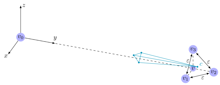
Figure 1: An example of the lower bound construction in dimension $d=3$. Observe that the convex hulls $\mathrm{Conv}\bigl{(}{v_{0},v_{1},v_{2}}\bigr{)}$, $\mathrm{Conv}\bigl{(}{v_{0},v_{1},v_{3}}\big{)}$, and $\mathrm{Conv}\bigl{(}{v_{0},v_{2},v_{3}}\bigr{)}$ only intersect in the node $v_{0}$, which corresponds to the $\mathit{SafeArea}$. Moreover, all other convex hulls of $3t$ nodes contain at least one of these three convex hulls. The light blue area shows the convex hull of all possible centroids $\mathrm{Conv}(\mathrm{S_{Cent}})$, where $c$ represents $\mathrm{Cent}^{\star}$. Observe that $v_{0}$ lies far away from $\mathrm{Ball(\mathrm{S_{Cent}})}$ in this figure.

∎

4.2 An optimal approximation of the centroid via the $\mathit{SafeArea}$ approach

In this section, we will show a simple algorithm that can achieve an optimal approximation of the true centroid. While the algorithm has a good approximation ratio, we show that it does not satisfy any validity condition, and therefore does not solve multidimensional approximate agreement according to Definition 3.1. This algorithm is based on the $\mathit{SafeArea}$ approach. In particular, the algorithm uses one preprocessing round where the nodes first calculate local approximations of the centroid. After computing local approximations of the centroid, the nodes use these vectors to establish multidimensional approximate agreement that satisfies the Containment condition. Algorithm 1 presents this idea in pseudocode.

Algorithm 1 Synchronous optimal approximation of the centroid for $n>\max(3t,(d+1)\cdot t)$

1:Each node $i$ in $[n]$ with input vector $v_{i}$ executes the following code:

2:     Broadcast $v_{i}$ reliably

3:     Reliably receive up to $n$ messages $M_{i}=\{v_{j},j\in[n]\}$

4:     Compute $\mathrm{S_{Cent}}(i)$ from all $v_{j}\in M_{i}$

5:     Set new vector $c_{i}$ to be the center of the smallest enclosing ball of $\mathrm{S_{Cent}}(i)$

6:     Run $\mathrm{SafeAlg}$ with input vector $c_{i}$

The $\mathrm{SafeAlg}$ subroutine used in Algorithm 1 is the synchronous version of Algorithm $6$ from [22]. It makes sure that the algorithm satisfies multidimensional approximate agreement with the Containment condition on the vectors $c_{i}$ with respect to Definition 3.1. Note that the vectors $c_{i}$ are not the same vectors as $v_{i}$, for which we cannot show the validity property. In the following, we show that Algorithm 1 converges, and the values on which the nodes terminate are an optimal approximation of the true centroid.

Theorem 4.4.

Algorithm 1 achieves an optimal approximation of $\mathrm{Cent}^{\star}$ in the synchronous setting. After $O\left(\log_{1/(1-\gamma)}\left(\frac{2}{\varepsilon}\cdot\mathrm{Rad\bigl{(}\mathrm{Ball(\mathrm{S_{Cent}})}\bigr{)}}\cdot\sqrt{d}\right)\right)$ synchronous rounds, the vectors of the correct nodes satisfy the $\varepsilon$-agreement property. The resilience of the algorithm is thereby $n>\max(3t,(d+1)t)$.

Observe that we only apply one round of reliable broadcast in the preprocessing step before executing $\mathrm{SafeAlg}$. Therefore, the resilience of our algorithm is $t<\max(n/3,n/(d+1))$ as in [22]. In the following, we show that the algorithm indeed converges to an optimal approximation of the centroid and that the convergence rate is not significantly larger than the convergence rate in [22].

Lemma 4.5.

Algorithm 1 outputs an optimal approximation of $\mathrm{Cent}^{\star}$.

Proof.

In Algorithm 1, during the first round, each correct node computes its local set of centroids $\mathrm{S_{Cent}}(i)\subseteq\mathrm{S_{Cent}}$. The set $\mathrm{S_{Cent}}$ itself cannot necessarily be computed by all correct nodes, since it is not guaranteed that they all receive $n$ messages. The set $\mathrm{S_{Cent}}(i)$ depends on the number of messages $|M_{i}|$ received by node $i$ during this first round. Using $\mathrm{S_{Cent}}(i)$, each node $i$ computes its local view of the smallest enclosing ball of this set $\mathrm{Ball}(\mathrm{S_{Cent}}(i))$, denoted by $\mathrm{Ball_{i}(\mathrm{S_{Cent}})}$. Note that $\mathrm{Ball_{i}(\mathrm{S_{Cent}})}\subseteq\mathrm{Ball(\mathrm{S_{Cent}})}$, since $\mathrm{S_{Cent}}(i)\subseteq\mathrm{S_{Cent}}$ for any correct node $i$. In particular, the radius of the local smallest enclosing ball is at most $\mathrm{Rad\bigl{(}\mathrm{Ball(\mathrm{S_{Cent}})}\bigr{)}}$. Moreover, each locally computed smallest enclosing ball contains $\mathrm{Cent}^{\star}$, i.e., for all true node $i$, $\mathrm{Cent}^{\star}\in\mathrm{Conv}(\mathrm{S_{Cent}}(i))\subseteq\mathrm{Ball}(\mathrm{S_{Cent}}(i))$. This holds because $M_{i}$ always contains all vectors from $n-f$ correct nodes (due to synchronous communication). Further, we can use the same argument as in 3.5, since $\mathrm{Cent}^{\star}$ can be written as a linear combination of elements of $\mathrm{S_{Cent}}(i)$. After the first round of Algorithm 1, each correct node $i$ therefore has a new input vector $c_{i}$ at a distance of at most $\mathrm{Rad\bigl{(}\mathrm{Ball(\mathrm{S_{Cent}})}\bigr{)}}$ away from $\mathrm{Cent}^{\star}$.

After the first round, the subroutine $\mathrm{SafeAlg}$ ensures that the final agreement vectors will be inside the convex hull of vectors $c_{i}$ that were computed in the first round. We denote this convex hull $\mathrm{Conv}_{c}$. Algorithm 1 therefore agrees inside $\mathrm{Conv}_{c}\coloneqq\mathrm{Conv}\left(\{c_{i}\mid\forall i\in[n]\text{ correct}\}\right)$.

Recall that every $c_{i}$ is at a distance of at most $\mathrm{Rad\bigl{(}\mathrm{Ball(\mathrm{S_{Cent}})}\bigr{)}}$ away from $\mathrm{Cent}^{\star}$, that is, for all correct $i\in[n]$, we get

$$\mathrm{dist}(c_{i},\mathrm{Cent}^{\star})\leq\mathrm{Rad\bigl{(}\mathrm{Ball(\mathrm{S_{Cent}})}\bigr{)}}.$$

Since $\mathrm{Conv}_{c}$ is a convex polytope, the distance to all vectors inside their convex hull can also be upper bounded by

$$\mathrm{dist}(x,\mathrm{Cent}^{\star})\leq\mathrm{Rad\bigl{(}\mathrm{Ball(\mathrm{S_{Cent}})}\bigr{)}}\quad\forall x\in\mathrm{Conv}_{c}.$$

Therefore, the approximation ratio of Algorithm 1 is

$$\frac{\max_{x\in\mathrm{Conv}_{c}}(x,\mathrm{Cent}^{\star})}{\mathrm{Rad\bigl{(}\mathrm{Ball(\mathrm{S_{Cent}})}\bigr{)}}}=1.$$

∎

It remains to argue about the convergence of the algorithm. The $\mathrm{SafeAlg}$ algorithm has a convergence ratio that depends on the maximum distance between any two true vectors. In the following, we show the convergence rate of Algorithm 1.

Lemma 4.6.

Algorithm 1 converges in $O\left(\log_{1/(1-\gamma)}\left(\frac{2}{\varepsilon}\cdot\mathrm{Rad\bigl{(}\mathrm{Ball(\mathrm{S_{Cent}})}\bigr{)}}\cdot\sqrt{d}\right)\right)$ rounds.

Proof.

Recall that, after one single round, all correct nodes have vectors $c_{i}$ that are inside $\mathrm{Ball(\mathrm{S_{Cent}})}$, indexing correct nodes with $i\in[n-f]$. Hence, after this first round, $\max_{\begin{subarray}{c}k\in[d]\\ i,j\in[n-f]\end{subarray}}|c_{i}[k]-c_{j}[k]|\leq 2\mathrm{Rad\bigl{(}\mathrm{Ball(\mathrm{S_{Cent}})}\bigr{)}}$. By [22], $\mathrm{SafeAlg}$ therefore converges in
$O\left(\log_{1/(1-\gamma)}\left(\frac{2}{\varepsilon}\cdot\mathrm{Rad\bigl{(}\mathrm{Ball(\mathrm{S_{Cent}})}\bigr{)}}\cdot\sqrt{d}\right)\right)$ rounds. ∎

This Lemma concludes the proof of Theorem 4.4. In the following, we discuss that the consensus vector from Algorithm 1 does not satisfy validity.

Observation 4.7.

The example in Figure 2 shows that Algorithm 1 does not satisfy the validity condition from Definition 3.1. Therefore, the Byzantine nodes can make the correct nodes agree on almost any vector.

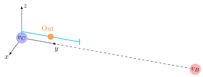
Figure 2: In the above example, suppose all correct nodes start with vector $v_{C}$ and all Byzantine nodes start with vector $v_{B}$. The segment in blue is the diameter of $\mathrm{Ball(\mathrm{S_{Cent}})}$ and the orange node $\mathrm{Out}$ is the output of every correct node if all of them receive all $n$ vectors. However, in order to satisfy the validity condition from Definition 3.1, the output of every correct node should be $v_{C}$.

4.3 A $\mathbf{2\sqrt{d}}$-approximation of the centroid with Box containment

In this section, we improve the approximation ratio as well as the resilience of the $\mathit{SafeArea}$ approach from Section 4.1. In addition, in contrast to the results in Section 4.2, we provide a solution for approximate multidimensional agreement. To this end, we relax the Containment condition from [22] to the weaker Box containment condition. We also restrict the area from which the nodes can choose their new vectors compared to the convex hull of $\mathrm{S_{Cent}}$ in Algorithm 1. The resulting Box containment condition is weaker than the Containment condition, and it is stronger than the standard validity condition.

Algorithm 2 shows a strategy that allows us to solve multidimensional approximate agreement with the Box containment. It provides an optimal resilience of $t<n/3$ and reaches a $2\sqrt{d}$ approximation of the true centroid while using polynomial local computation time. Thus, the algorithm outperforms the $\mathit{SafeArea}$ approach in resilience, consensus quality, and computation time. The idea of Algorithm 2 is to compute a box containing trusted values and a box containing all possible centroids. In every round, the new input vector is set to be the midpoint of the intersection area of the two boxes.

Definition 4.8 (Centroid box).

We define the centroid box CB to be the smallest box containing $\mathrm{S_{Cent}}$, and the local centroid box $\textrm{CB}_{i}$ of node $i\in[n]$ to be the smallest box containing $\mathrm{S_{Cent}}(i)$.

In the following, we make the observation that the local Centroid box can be indeed computed in polynomial time locally:

Observation 4.9.

CB can be computed in polynomial time as follows: for each coordinate, compute the average of the $n-t$ smallest values and the average of the $n-t$ largest values. This yields the interval defining the box over this coordinate.

We next define the midpoint function, which is used in the algorithm.

Definition 4.10 (Midpoint).

The $\mathrm{Midpoint}$ of a box $X$ is defined as follows:

$$\mathrm{Midpoint}(X)=\Bigl{(}\mathrm{Midpoint}\bigl{(}X[1]\bigr{)},\dots,\mathrm{Midpoint}\bigl{(}X[d]\bigr{)}\Bigr{)},$$

where $X[k]$ is the set containing all $k^{th}$ coordinates of vectors of the set $X$, and the one-dimensional $\mathrm{Midpoint}$ function returns the midpoint of the interval spanned by a finite multiset of real values.

In order to analyze the convergence of the algorithm, we will define the convergence rate with respect to the longest edges of the boxes, which are defined as follows:

Definition 4.11 (Length of the longest edge ($\mathcal{LE}$)).

The length of the longest edge of a box $B$ is defined as

$$\mathcal{LE}(B\,)=\max_{\begin{subarray}{c}k\in[d]\\ u,v\in B\end{subarray}}\bigl{|}u[k]-v[k]\bigr{|}.$$

Note that $\mathcal{LE}(\textrm{TB}\,)=\max_{\begin{subarray}{c}k\in[d]\\ i,j\in[n-f]\end{subarray}}\bigl{|}v_{i}[k]-v_{j}[k]\bigr{|},$ where $i\in[n-f]$ are the indices of the true vectors, and the longest edge thus corresponds to the diameter of the true vectors.

The following theorem shows the main properties of the algorithm.

Algorithm 2 Synchronous approximate agreement with Box containment, $n>3\cdot t$

1:In each round $r=1,2,\ldots$, each node $i$ in $[n]$ with input vector $v_{i}$ executes the following code:

2:     Broadcast $v_{i}$ reliably

3:     Reliably receive up to $n$ messages $M_{i}=\{v_{j},j\in[n]\}$

4:     Compute $\textrm{TB}_{i}$ and $\textrm{CB}_{i}$ from $M_{i}$ by excluding $|M_{i}|-(n-t)$ values on each side

5:     Set $v_{i}$ to $\mathrm{Midpoint}(\textrm{TB}_{i}\cap\textrm{CB}_{i})$.

Theorem 4.12.

Algorithm 2 achieves a $2\sqrt{d}$-approximation of $\mathrm{Cent}^{\star}$ in the synchronous setting. After $O\Bigl{(}\log\bigl{(}\frac{1}{\varepsilon}\cdot\mathcal{LE}\left(\textrm{TB}\right)\bigr{)}\Bigr{)}$ synchronous rounds, the vectors of the correct nodes satisfy multidimensional approximate agreement with Box containment. The resilience of the algorithm is thereby $n>3\cdot t$.

In the following, we prove the correctness of Theorem 4.12 in several steps. We start by showing that Algorithm 2 is well-defined, by showing that $\textrm{TB}_{i}$ and $\textrm{CB}_{i}$ intersect if $n>2t$. This way, all correct nodes are able to choose a new input vector in line 5 of Algorithm 2.

Lemma 4.13.

For all correct nodes $i$, the local trusted box and the local centroid box have a non-empty intersection: $\textrm{CB}_{i}\cap\textrm{TB}_{i}\neq\emptyset$.

Proof.

Let $\textrm{TB}_{i}[k]$ and $\textrm{CB}_{i}[k]$ be the (coordinate-wise) projections of $\textrm{TB}_{i}$ and $\textrm{CB}_{i}$ on the $k^{th}$ coordinate, respectively. We prove the statement of the lemma for some correct node $i$ (note that this proof works for every correct node).

For each coordinate $k\in[d]$, let $v_{j}[k]$ denote the $k^{th}$ coordinate of the vector received from node $j$. We order the values $v_{j}[k],\forall k\in[n]$ as in 3.10. Recall that node $i$ receives $m_{i}\geq n-t$ vectors and therefore there are $m_{i}$ values in each coordinate. Because we remove $m_{i}-(n-t)$ on each side of the interval for each coordinate $k$, each $\textrm{TB}_{i}[k]$ contains $2(n-t)-m_{i}\geq n-2t$ values. Our goal is to construct a point that is both in $\textrm{TB}_{i}$ and $\textrm{CB}_{i}$.

Consider the averaged sum $c_{l}$ of the $n-t$ smallest received values in coordinate $k$: $c_{l}=\frac{1}{n-t}\sum_{j=1}^{n-t}v_{j}[k]$. Observe that there exists a subset of $n-t$ vectors with this averaged sum in their $k^{th}$ coordinate. The corresponding vector is the centroid of the $n-t$ nodes with these input vectors. Similarly, there exists an averaged sum $c_{u}=\frac{1}{n-t}\sum_{j=m_{i}-(n-t)+1}^{m_{i}}v_{j}[k]\in\mathrm{S_{Cent}}[k]$ formed by the $n-t$ largest values in coordinate $k$, that corresponds to the $k^{th}$ coordinate of some centroid.

Let $V_{k}=\frac{1}{2(n-t)-m_{i}}\sum_{j=m_{i}-(n-t)+1}^{n-t}v_{j}[k]$ be the average of values, where we truncate the $m_{i}-(n-t)$ smallest and largest values in this coordinate. This is possible since $t<n/3$ and $m_{i}\geq n-t$. Since the values $v_{j}[k]$ are ordered, $\frac{1}{2(n-t)-m_{i}}\sum_{j=m_{i}-(n-t)+1}^{n-t}v_{j}[k]\geq c_{l}$ and $\frac{1}{2(n-t)-m_{i}}\sum_{j=m_{i}-(n-t)+1}^{n-t}v_{j}[k]\leq c_{u}$. Therefore, $V_{k}\in[c_{l},c_{u}]\subseteq\textrm{CB}_{i}[k]$. Also, $V_{k}\in\bigl{[}v_{m_{i}-(n-t)+1}[k],v_{n-t}[k]\bigr{]}=\textrm{TB}_{i}[k]$, since it is the mean of values $v_{m_{i}-(n-t)+1}[k]$ to $v_{n-t}[k]$.

Now, consider a vector $V$ s.t. $\forall k\in[d]$: $V[k]=V_{k}$. By the definitions of $\textrm{TB}_{i}$ and $\textrm{CB}_{i}$, since $V[k]\in\textrm{TB}_{i}[k]\cap\textrm{CB}_{i}[k],\forall k\in[d]$, this vector will be inside the intersection of the boxes, i.e. $V\in\textrm{TB}_{i}\cap\textrm{CB}_{i}$. ∎

Lemma 4.14.

Algorithm 2 converges.

Proof.

We start by defining TB and $\textrm{TB}_{i}$ with respect to rounds $r$ of the algorithm. The initial $\textrm{TB}=\textrm{TB}^{1}$ is the smallest box containing all true vectors. Let $\textrm{TB}^{r+1}$ be the smallest box that contains all the vectors computed by correct nodes in round $r$, which will represent the input in round $r+1$. Observe that during a round $r$, each node $i$ computes $\textrm{TB}_{i}^{r}\subseteq\textrm{TB}^{r}$, and picks its new vector inside this box.

In order to prove convergence, we need to show that the vectors computed in each round are getting closer together. In particular, we show that for any two correct nodes $i$ and $j$, and the corresponding local boxes $\textrm{TB}_{i}^{r}$ and $\textrm{CB}_{i}^{r}$ computed in some round $r\geq 1$, the following inequality is satisfied:

$$\bigl{|}\mathrm{Midpoint}(\textrm{TB}_{i}^{r}\cap\textrm{CB}_{i}^{r})-\mathrm{Midpoint}(\textrm{TB}_{j}^{r}\cap\textrm{CB}_{j}^{r})\bigr{|}\leq\delta\cdot\mathcal{LE}(\textrm{TB}^{r}),$$

where $\delta<1$ is a small constant.

We first show that $\textrm{TB}_{i}^{r}\subseteq\textrm{TB}^{r}$: At the beginning of round $r$, $\textrm{TB}^{r}$ is the smallest box containing all true vectors. Let us consider the boxes with respect to one coordinate $k\in[d]$. If the interval $\textrm{TB}_{i}^{r}[k]$ does not contain any Byzantine values, then $\textrm{TB}_{i}^{r}[k]\subseteq\textrm{TB}^{r}[k]$ by definition. This could have either happened if the node only received true vectors, or if the Byzantine values were removed as extreme values when computing the interval $\textrm{TB}_{i}^{r}[k]$. Otherwise, we assume that the interval $\textrm{TB}_{i}^{r}[k]$ contains at least one Byzantine value. This implies that, when the $m_{i}-(n-t)$ smallest and largest values were removed, this Byzantine value remained inside the interval $\textrm{TB}_{i}^{r}[k]$, and at least two true values were removed instead (one on each side of the interval) since there are at most $m_{i}-(n-t)$ Byzantine values in $M_{i}[k]$. Therefore, $\textrm{TB}_{i}^{r}[k]$ is included in an interval bounded by two true values, which is by definition included in $\textrm{TB}^{r}[k]$. Since this holds for each coordinate $k$, it also holds that $\textrm{TB}_{i}^{r}\subseteq\textrm{TB}^{r}$.

Next, we use 3.10 to sort the received values for each coordinate $k$. For node $i$, we define the locally trusted box in coordinate $k$ as $\textrm{TB}_{i}^{r}[k]=\bigl{[}v_{m_{i}-(n-t)+1}[k],v_{n-t}[k]\bigr{]}$, and for node $j$ as $\textrm{TB}_{j}^{r}[k]=\bigl{[}v^{\prime}_{m_{i}-(n-t)+1}[k],v^{\prime}_{n-t}[k]\bigr{]}$. Let $t_{l}$ denote the smallest and $t_{u}$ the largest true value in coordinate $k$ (given all true vectors). Since $\textrm{TB}_{i}^{r}[k]\subseteq\textrm{TB}^{r}[k]$, $v_{m_{i}-(n-t)+1}[k]\geq t_{l}$ and $v_{n-t}[k]\leq t_{u}$. Similarly, $v^{\prime}_{m_{i}-(n-t)+1}[k]\geq t_{l}$ and $v^{\prime}_{n-t}[k]\leq t_{u}$. Moreover, since Byzantine parties could be inside TB, $\textrm{TB}_{i}[k]$ and $\textrm{TB}_{j}[k]$ could have been computed by removing up to $m_{i}-(n-t)$ true values on each side. Let $t_{1}$ denote the $(m_{i}-(n-t)+1)^{th}$ true value and $t_{2}$ the $(2n-f-t-m_{i})^{th}$ true value in coordinate $k$ (recall there are $n-f$ true values in total), these true values are necessarily inside both $\textrm{TB}_{i}[k]$ and $\textrm{TB}_{j}[k]$.

Then, $v_{m_{i}-(n-t)+1}[k]\leq t_{1}$ and $v_{n-t}[k]\geq t_{2}$. Similarly, $v^{\prime}_{m_{i}-(n-t)+1}[k]\leq t_{1}$ and $v^{\prime}_{n-t}[k]\geq t_{2}$. We can now upper bound the distance between the computed midpoints of the nodes $i$ and $j$.

$$\Bigl{|}\mathrm{Midpoint}\bigl{(}\textrm{TB}_{i}^{r}[k]\bigr{)}-\mathrm{Midpoint}\bigl{(}\textrm{TB}_{j}^{r}[k]\bigr{)}\Bigr{|} \leq\frac{t_{u}-t_{1}}{2}-\frac{t_{2}-t_{l}}{2}\leq\frac{t_{u}-t_{l}}{2}$$

$$\leq\frac{\mathcal{LE}(\textrm{TB}^{r})}{2}$$

This inequality holds for every pair of nodes $i$ and $j$ and therefore we get

$$\max_{i,j\in[n]}\Bigl{|}\mathrm{Midpoint}\bigl{(}\textrm{TB}_{i}^{r}[k]\bigr{)}-\mathrm{Midpoint}\bigl{(}\textrm{TB}_{j}^{r}[k]\bigr{)}\Bigr{|} \leq\frac{\mathcal{LE}(\textrm{TB}^{r})}{2}$$

$$\Leftrightarrow\mathcal{LE}\bigl{(}\textrm{TB}^{r+1}[k]\bigr{)} \leq\frac{\mathcal{LE}(\textrm{TB}^{r})}{2}$$

for each coordinate $k$.

After $R$ rounds, $\mathcal{LE}(\textrm{TB}^{R})\leq\frac{1}{2^{R}}\cdot\mathcal{LE}(\textrm{TB})$ holds. Since there exists $R\in\mathbb{N}$ s.t.
$\frac{1}{2^{R}}\cdot\mathcal{LE}(\textrm{TB})\leq\varepsilon$, the algorithm converges.

∎

Lemma 4.15.

After $\Bigl{\lceil}\log\bigl{(}\frac{1}{\varepsilon}\cdot\mathcal{LE}(\textrm{TB})\bigr{)}\Bigr{\rceil}$ synchronous rounds of Algorithm 2, the correct nodes hold vectors that are at a distance $\varepsilon$ from each other.

Proof.

As shown in the proof of Lemma 4.14, after $R$ rounds, $\mathcal{LE}(\textrm{TB}^{R})\leq\frac{1}{2^{R}}\cdot\mathcal{LE}(\textrm{TB})$. The statement therefore holds for $R=\Bigl{\lceil}\log\bigl{(}\frac{1}{\varepsilon}\cdot\mathcal{LE}(\textrm{TB})\bigr{)}\Bigr{\rceil}$. ∎

Observe that, with Lemma 4.14 and Lemma 4.15, Algorithm 2 can be adjusted such that the nodes terminate after $\Bigl{\lceil}\log\bigl{(}\frac{1}{\varepsilon}\cdot\mathcal{LE}(\textrm{TB})\bigr{)}\Bigr{\rceil}$ synchronous rounds. This can be achieved by letting the nodes mark their last sent message, such that other nodes can use this last vector for future computations. This way, the algorithm satisfies $\varepsilon$-agreement and termination. The following lemma shows that the algorithm satisfies Box containment.

Lemma 4.16.

Algorithm 2 satisfies Box containment.

Proof.

Observe that each correct node $i$ always picks a new vector inside $\textrm{TB}_{i}$. The set of locally received vectors depends on the received messages $M_{i}$. In the proof of Lemma 4.14, we showed that $\textrm{TB}_{i}^{r}\subseteq\textrm{TB}^{r}$ for all rounds $r$. This also means that $\textrm{TB}_{i}^{r}\subseteq\textrm{TB}^{1}=\textrm{TB}$ always holds. Hence, $\textrm{TB}_{i}^{r}\subseteq\textrm{TB}$ holds for all $i$ and $r$. This implies that the vectors converge towards a vector inside TB. ∎

Observe that the algorithm also trivially satisfies the validity condition, and therefore solves multidimensional approximate agreement.

Observation 4.17.

By agreeing inside TB, Algorithm 2 satisfies the validity condition.

Next, we show that Algorithm 2 provides a $2\sqrt{d}$ approximation of the true centroid.

Lemma 4.18.

The approximation ratio of the true centroid by Algorithm 2 is upper bounded by $2\sqrt{d}$.

Proof.

Following Definition 3.8, we need to show that the ratio between the distance from any output of Algorithm 2 to $\mathrm{Cent}^{\star}$ and the optimal radius $\mathrm{Rad\bigl{(}\mathrm{Ball(\mathrm{S_{Cent}})}\bigr{)}}$ is less than $2\sqrt{d}$.

We first lower bound the radius of the smallest enclosing ball of $\mathrm{S_{Cent}}$. Observe that the radius is always at least $\max_{x,y\in\mathrm{S_{Cent}}}\bigl{(}\mathrm{dist}(x,y)\bigr{)}/2$.

Next, we focus on upper bounding the distance between $\mathrm{Cent}^{\star}$ and the furthest possible point from it inside CB. W.l.o.g., we assume that $\max_{x,y\in\mathrm{S_{Cent}}}\bigl{(}\mathrm{dist}(x,y)\bigr{)}=1$. We consider the relation between the smallest enclosing ball and CB. Observe that each face of the box CB has to contain at least one point of $\mathrm{S_{Cent}}$. If CB is contained inside the ball, i.e. if the vertices of the box would lie on the ball surface, the computed approximation of Algorithm 2 would always be optimal.

The worst case is achieved if the ball is (partly) contained inside CB. Then, the optimal solution might lie inside CB and the ball, while the furthest node may lie on one of the vertices of CB outside of the ball. The distance of any node from $\mathrm{Cent}^{\star}$ in this case is upper bounded by the diagonal of the box. Since the longest distance between any two points was assumed to be $1$, the box is contained in a unit cube. Thus, the largest distance between two points of CB is at most $\sqrt{d}$.

The approximation ratio of Algorithm 2 can be upper bounded by:

$$\frac{\max_{x\in\textrm{CB}}\bigl{(}\mathrm{dist}(\mathrm{Cent}^{\star},x)\bigr{)}}{\mathrm{Rad\bigl{(}\mathrm{Ball(\mathrm{S_{Cent}})}\bigr{)}}}\leq 2\cdot\frac{\max_{x\in\textrm{CB}}\bigl{(}\mathrm{dist}(\mathrm{Cent}^{\star},x)\bigr{)}}{\max_{x,y\in\mathrm{S_{Cent}}}\bigl{(}\mathrm{dist}(x,y)\bigr{)}}\leq 2\cdot\frac{\sqrt{d}}{1}=2\sqrt{d}.$$

∎

Lemma 4.19.

Algorithm 2 can tolerate up to $t$ Byzantine parties where $n>3t$.

Proof.

In Lemma 4.13, we discuss that $\textrm{CB}_{i}\cap\textrm{TB}_{i}\neq\emptyset$. This proof in fact requires an upper bound of $t<n/2$ on the number of Byzantine nodes. The required upper bound of $t<n/3$ on the number of Byzantine nodes comes from the implementation of reliable broadcast as a subroutine. This property is implicitly used to ensure that the set $\mathrm{S_{Cent}}$ is bounded in size by $\binom{n}{n-t}$ and cannot be extended to an arbitrarily large size by Byzantine parties. ∎

This lemma concludes the proof of Theorem 4.12 and the analysis of the centroid approximation for the synchronous case.

5 Asynchronous algorithms for approximate computation of the centroid

In the asynchronous case, the nodes cannot rely on the fact that they receive vectors from all correct nodes. In every round, a node can only wait for up to $n-t$ vectors. Therefore, only $n-2t$ of the vectors can be guaranteed to come from the correct nodes. Due to this restriction, also the definitions of the $\mathit{SafeArea}$ as well as the local trusted boxes need to be adjusted.

The asynchronous multidimensional approximate agreement algorithm from [22] is also based on the $\mathit{SafeArea}$ approach. In the asynchronous case, the $\mathit{SafeArea}$ that is computed is slightly different. The smaller convex hulls of $n-2t$ nodes are considered for the intersection. This decreases the number of Byzantine parties that are tolerated to $t<n/(d+2)$. The decrease is necessary for the $\mathit{SafeArea}$ to be non-empty. The asynchronous $\mathit{SafeArea}$ is defined as follows:

Definition 5.1 (Asynchronous $\mathit{SafeArea}$).

In the asynchronous setting, the $\mathit{SafeArea}$ of a set of vectors $\{v_{i},i\in\left[n\right]\}$ that can contain up to $t$ Byzantine vectors is defined as

$$\mathit{SafeArea}=\bigcap_{\begin{subarray}{c}I\subseteq\left[n\right]\\ |I|=n-2t\end{subarray}}\mathrm{Conv}\bigl{(}\{v_{i},i\in I\}\bigr{)}.$$

Also, the trusted box that the nodes can compute locally is reduced in size. In the following, we redefine the local trusted box for asynchronous communication:

Definition 5.2 (Asynchronous local trusted box).

For all received vectors from nodes $i\in[n-t]$, denote $v_{i}[k]$ the $k^{th}$ coordinate of the respective vector. Assume that all $v_{i}[k]$ are sorted and relabeled as in 3.10. Then, in the asynchronous case, the locally computed trusted box $\widetilde{\textrm{TB}_{i}}$ is defined as

$$\widetilde{\textrm{TB}_{i}}[k]=\bigl{[}v_{t+1}[k],v_{n-2t}[k]\bigr{]},\ \forall k\in[d].$$

5.1 Approximation through the asynchronous $\mathit{SafeArea}$ approach

As before, we start by discussing the lower bound on the approximation of the asynchronous $\mathit{SafeArea}$ approach. Compared to the synchronous case, the Byzantine adversary is able to additionally hide up to $t$ true vectors from the correct nodes.

Theorem 5.3.

The approximation ratio of the asynchronous multidimensional approximate agreement via the $\mathit{SafeArea}$ approach, where the $\mathit{SafeArea}$ is a single vector, is lower bounded by $2(d+1)$.

Proof.

In this proof, we will extend the example in the proof of Theorem 4.3. Since the Byzantine adversary can hide up to $t$ true vectors, we can assume that the $t$ hidden nodes lie far away from the locally computed $\mathit{SafeArea}$. If they lie too far, they can increase the radius of the smallest enclosing ball and thus improve the approximation ratio. Therefore, we assume that the $t$ hidden true vectors lie in $(x,\ldots,0)$.

We can replace $d$ by $d+1$ in the calculations from Theorem 4.3 and arrive at a lower bound of $2(d+1)$ for the approximation ratio of the asynchronous $\mathit{SafeArea}$ approach. ∎

5.2 A $2$-approximation of the centroid via the $\mathit{SafeArea}$ approach

Similar to Section 4.2, we can achieve a good approximation of $\mathrm{Cent}^{\star}$ without satisfying the validity property of multidimensional approximate agreement in the asynchronous case.

In the asynchronous case, every node can only wait for $n-t$ other vectors. If Byzantine vectors are among the received messages, a correct node will not be able to compute an optimal approximation of $\mathrm{Cent}^{\star}$ locally. This is because the average of the $n-t$ received vectors does not need to be $\mathrm{Cent}^{\star}$. Instead, each node can only compute one possible centroid from $\mathrm{S_{Cent}}$. Algorithm 3 presents this idea in pseudocode. The next theorem shows that the computation of one centroid is sufficient to achieve a $2$-approximation of $\mathrm{Cent}^{\star}$.

Algorithm 3 Asynchronous $2$-approximation of the centroid for $n>(d+2)\cdot t$

1:Each node $i$ in $[n]$ with input vector $v_{i}$ executes the following code:

2:     Broadcast own vector $v_{i}$ reliably

3:     upon Reliably receiving $n-t$ vectors $v_{j}$ do

4:         $c_{i}\leftarrow$ centroid of the received $v_{j}$

5:         Run $\mathrm{SafeAlg}$ with input vector $c_{i}$

6:     end upon

Theorem 5.4.

Algorithm 3 achieves a $2$-approximation of $\mathrm{Cent}^{\star}$ in an asynchronous setting. After $O\left(\log_{1/(1-\gamma)}\left(\frac{1}{\varepsilon}\cdot\mathrm{Rad\bigl{(}\mathrm{Ball(\mathrm{S_{Cent}})}\bigr{)}}\cdot\sqrt{d}\right)\right)$ asynchronous rounds, the vectors of the correct nodes converge. The resilience of the algorithm is thereby $n>(d+2)t$.

Proof.

When computing the centroid of $n-t$ values, each node $i$ computes one element of $\mathrm{S_{Cent}}$. This ensures that the algorithm agrees inside $\mathrm{Ball(\mathrm{S_{Cent}})}$. The maximum distance between any vector in $\mathrm{Conv}(\mathrm{S_{Cent}})$ and $\mathrm{Cent}^{\star}$ is the diameter of $\mathrm{Ball(\mathrm{S_{Cent}})}$, which is twice the radius $\mathrm{Rad\bigl{(}\mathrm{Ball(\mathrm{S_{Cent}})}\bigr{)}}$. Therefore, Algorithm 3 outputs a $2$-approximation of $\mathrm{Cent}^{\star}$. Since the only difference of this algorithm from Algorithm 1 is the preprocessing step, the remaining properties of the algorithm follow from the proof of Theorem 4.4. ∎

5.3 A $4\sqrt{d}$-approximation of the centroid with Box containment

At the beginning of Section 5, we redefined the local trusted box for the asynchronous case. Note that the local trusted box in the asynchronous case is just smaller than in the synchronous case, and is still included in TB. Observe that this is not true for the centroid box. In the asynchronous case, each correct node can only compute one vector from $\mathrm{S_{Cent}}$, and therefore $\textrm{CB}_{i}$ would be just containing one point. In order to derive similar convergence results to the synchronous case, we need to relax the definition of CB. This relaxation will lead to a worse approximation ratio in the asynchronous case.

Definition 5.5 (Relaxation of CB).

We define $\widetilde{\textrm{CB}}$ to be the smallest box containing all possible centroids of $n-2t$ vectors:

$$\widetilde{\textrm{CB}}=\mathrm{Conv}\left(\left\{\frac{1}{n-2t}\sum_{i\in I}v_{i}\ \bigg{|}\ \forall I\subseteq[n],|I|=n-2t\right\}\right),$$

and $\widetilde{\textrm{CB}}_{i}$ is defined to be the smallest local box containing all possible centroids of $n-2t$ vectors, formed from the vectors received by node $i$:

$$\widetilde{\textrm{CB}}_{i}=\mathrm{Conv}\left(\left\{\frac{1}{n-2t}\sum_{v\in V}v\ \bigg{|}\ \forall V\subseteq M_{i},|V|=n-2t\right\}\right),$$

where $M_{i}$ is the set of vectors received by node $i$.

With these definitions, we can now present an algorithm solving asynchronous approximate multidimensional agreement with Box containment. The algorithm is similar to Algorithm 2, with the difference that the nodes choose their new vector inside $\widetilde{\textrm{TB}_{i}}\cap\widetilde{\textrm{CB}}_{i}$. We will assume that each node receives exactly $n-t$ vectors in each round. Though a node may receive more vectors in a round, the additional vectors can be ignored by the algorithm. Algorithm 4 presents this strategy in pseudocode.

Algorithm 4 Asynchronous approximate agreement with Box containment, $n>3\cdot t$

1:Each node $i$ in $[n]$ with input vector $v_{i}$ executes the following code:

2:Set local round $r\leftarrow 0$

3:while true do

4:     $r\leftarrow r+1$

5:     Broadcast $(v_{i},r)$ reliably

6:     upon Receiving $n-t$ values $v_{j}$ in round $r$ reliably do

7:         Set $M_{i}\leftarrow$ received $(v_{j},r)$

8:         Compute $\widetilde{\textrm{TB}_{i}}$ and $\widetilde{\textrm{CB}}_{i}$ from $M_{i}$ by excluding $t$ smallest and $t$ largest values in each coordinate

9:         Set $v_{i}$ to $\mathrm{Midpoint}(\widetilde{\textrm{TB}_{i}}\cap\widetilde{\textrm{CB}}_{i})$

10:     end upon

11:end while

Before diving into the analysis of the algorithm, we make the following observations:

Observation 5.6.

The following properties hold:

• $\textrm{CB}\subseteq\widetilde{\textrm{CB}}$ (by Definition 5.5),

• The intersection $\widetilde{\textrm{TB}_{i}}\cap\textrm{CB}_{i}$ can be empty

• $\widetilde{\textrm{CB}}_{i}\subseteq\widetilde{\textrm{CB}}$.

The following theorem describes the properties of Algorithm 4:

Theorem 5.7.

Algorithm 4 achieves a $4\sqrt{d}$-approximation of $\mathrm{Cent}^{\star}$ in an asynchronous setting. After $O\Bigl{(}\log\left(\frac{1}{\varepsilon}\cdot\mathcal{LE}(\textrm{TB})\right)\Bigr{)}$ asynchronous rounds, the vectors of the correct nodes converge. The resilience of the algorithm is thereby $n>3t$.

We will show this theorem in several steps. Observe first that the number of rounds of the algorithm can be derived analogously to the proof of Lemma 4.15. We start by showing that the algorithm is correct and converges. From this, one can derive that the solution satisfies Box containment. Therefore, Algorithm 4 solves multidimensional approximate agreement. The required resilience for the analysis is $t<n/3$. We will skip the proofs of some of these statements, since they are equivalent to the proofs in Section 4.3. In the second part, we show that the approximation ratio of the algorithm is upper bounded by $4\sqrt{d}$.

Lemma 5.8.

Algorithm 4 is well-defined and converges.

Proof.

We start by showing that Algorithm 4 is well-defined. We therefore need to prove that $\widetilde{\textrm{TB}_{i}}\cap\widetilde{\textrm{CB}}_{i}\neq\emptyset$.

Consider $\widetilde{\textrm{TB}_{i}}[k]$ and $\widetilde{\textrm{CB}}_{i}[k]$ to be the projections of $\widetilde{\textrm{TB}_{i}}$ and $\widetilde{\textrm{CB}}_{i}$ on the $k^{th}$ coordinate respectively. Note that $\widetilde{\textrm{TB}_{i}}$ is always computed from at least $n-t$ received messages. In order to compute $\widetilde{\textrm{TB}_{i}}$, a node would remove $t$ values “on each side” for each coordinate $k\in[d]$. For each coordinate $k\in[d]$, we denote by $v_{j}[k]$ the $k^{th}$ coordinate of the vector that could be received from node $j$. As in previous proofs, we reorder the values $v_{j}[k]$ and reassign the indices according to 3.10. Now we can rewrite $\widetilde{\textrm{TB}_{i}}[k]=\bigl{[}v_{t+1}[k],v_{n-2t}[k]\bigr{]}$.

Consider the average vector $c_{l}=\frac{1}{n-2t}\sum_{j=1}^{n-2t}v_{j}[k]$. Since it corresponds to a sum of the $k^{th}$ coordinates of a set of $n-2t$ vectors, there exists a centroid in $\mathrm{S_{Cent}}$ s.t. the $k^{th}$ coordinate is $c_{l}=\frac{1}{n-2t}\sum_{j=1}^{n-2t}v_{j}[k]$. Similarly, $\exists\ c_{u}=\frac{1}{n-2t}\sum_{j=t+1}^{n-t}v_{j}[k]\in\mathrm{S_{Cent}}[k]$.

Since the values $v_{j}[k]$ are in increasing order, $\frac{1}{n-3t}\sum_{j=t+1}^{n-2t}v_{j}[k]\geq c_{l}$ and $\frac{1}{n-3t}\sum_{j=t+1}^{n-2t}v_{j}[k]\leq c_{u}$. We define $V_{k}=\frac{1}{n-3t}\sum_{j=t+1}^{n-2t}v_{j}[k]$. Note that $V_{k}\in[c_{l},c_{u}]\subseteq\widetilde{\textrm{CB}}_{i}[k]$, since $\widetilde{\textrm{CB}}_{i}$ is a convex polytope. Also, $V_{k}\in\bigl{[}v_{t+1}[k],v_{n-2t}[k]\bigr{]}=\widetilde{\textrm{TB}_{i}}[k]$, since it is the mean of values $v_{t+1}[k]$ to $v_{n-2t}[k]$.

Now, consider the vector $V$ s.t. $\forall k\in[d]$, $V[k]=V_{k}$. By definition of $\widetilde{\textrm{TB}_{i}}$ and $\widetilde{\textrm{CB}}_{i}$, since $V[k]\in\widetilde{\textrm{TB}_{i}}[k]\cap\widetilde{\textrm{CB}}_{i}[k],\forall k\in[d]$, $V\in\widetilde{\textrm{TB}_{i}}\cap\widetilde{\textrm{CB}}_{i}$. This concludes the proof of the algorithm being well-defined.

The proof of convergence is the same as in the proof of Lemma 4.14 since only TB was used to prove convergence and not CB. ∎

To prove an upper bound on the approximation ratio of Algorithm 4, we need the following intermediate lemma, which allows us to use Lemma 4.18 for the upper bound proof.

Lemma 5.9.

The diagonal of $\widetilde{\textrm{CB}}$ is at most twice the diagonal of CB.

Proof.

Note that the boxes CB and $\widetilde{\textrm{CB}}$ cannot be computed locally, but the locally computed boxes $\textrm{CB}_{i}$ and $\widetilde{\textrm{CB}}_{i}$ are included in CB and $\widetilde{\textrm{CB}}$ respectively. We consider coordinate $k$, and assume that the values $v_{i}[k]$ are indexed so that they are in increasing order (see 3.10). Denote $\mathrm{Edge}\bigl{(}\textrm{CB}[k]\bigr{)}$ the length of the interval $\textrm{CB}[k]$. Then, the length of $\textrm{CB}[k]$ is,

$$\mathrm{Edge}\bigl{(}\textrm{CB}[k]\bigr{)} =\frac{1}{n-t}\sum_{i=t+1}^{n}v_{i}[k]-\frac{1}{n-t}\sum_{i=1}^{n-t}v_{i}[k]=\frac{1}{n-t}\sum_{i=1}^{t}v_{i}[k]+\frac{1}{n-t}\sum_{i=n-t+1}^{n}v_{i}[k]$$

$$\geq\frac{1}{n-t}\left[\sum_{i=1}^{2t}v_{i}[k]+\sum_{i=n-2t+1}^{n}v_{i}[k]\right].$$

And the length of $\widetilde{\textrm{CB}}[k]$ is,

$$\mathrm{Edge}\bigl{(}\widetilde{\textrm{CB}}[k]\bigr{)} =\frac{1}{n-2t}\sum_{i=2t+1}^{n}v_{i}[k]-\frac{1}{n-2t}\sum_{i=1}^{n-2t}v_{i}[k]=\frac{1}{n-2t}\left[\sum_{i=1}^{2t}v_{i}[k]+\sum_{i=n-2t+1}^{n}v_{i}[k]\right].$$

Denote $a=\sum_{i=1}^{2t}v_{i}[k]$ and $b=\sum_{i=n-2t+1}^{n}v_{i}[k]$. Then,

$$\frac{\mathrm{Edge}\bigl{(}\widetilde{\textrm{CB}}[k]\bigr{)}}{\mathrm{Edge}\bigl{(}\textrm{CB}[k]\bigr{)}}\leq\frac{\frac{1}{n-2t}\cdot a+\frac{1}{n-2t}\cdot b}{\frac{1}{n-t}\cdot a+\frac{1}{n-t}\cdot b}\leq\frac{\frac{2}{n-t}\cdot a+\frac{2}{n-t}\cdot b}{\frac{1}{n-t}\cdot a+\frac{1}{n-t}\cdot b}=2,$$

since $n\geq 3t\Leftrightarrow\frac{1}{n-2t}\leq\frac{2}{n-t}$.

Observe that, since this inequality is true for every coordinate $k$, it also holds for the diagonals of the boxes CB and $\widetilde{\textrm{CB}}$.

∎

Lemma 5.10.

The approximation ratio of Algorithm 4 is upper bounded by $4\sqrt{d}$.

Proof.

We can lower bound the radius of the enclosing ball by $\max_{x,y\in\mathrm{S_{Cent}}}\bigl{(}\mathrm{dist}(x,y)\bigr{)}/2$, as in the proof of Lemma 4.18.

Observe that Algorithm 4 does not converge inside CB, but inside $\widetilde{\textrm{CB}}$. The furthest Algorithm 4 can get from $\mathrm{Cent}^{\star}$ is then $\max_{x\in\widetilde{\textrm{CB}}}(\mathrm{dist}\bigl{(}\mathrm{Cent}^{\star},x)\bigr{)}$. Assume w.l.o.g. that the longest edge of CB is $1$. Since $\textrm{CB}\subseteq\widetilde{\textrm{CB}}$ (5.6) and the diagonal of $\widetilde{\textrm{CB}}$ is at most twice the diagonal of CB (Lemma 4.14), the furthest distance is upper bounded by

$$\max_{x\in\widetilde{\textrm{CB}}}\bigl{(}\mathrm{dist}(\mathrm{Cent}^{\star},x)\bigr{)}\leq 2\max_{x\in\textrm{CB}}\bigl{(}\mathrm{dist}(\mathrm{Cent}^{\star},x)\bigr{)}.$$

Therefore, the approximation ratio is upper bounded by

$$\frac{\max_{x\in\widetilde{\textrm{CB}}}\bigl{(}\mathrm{dist}(\mathrm{Cent}^{\star},x)\bigr{)}}{\mathrm{Rad\bigl{(}\mathrm{Ball(\mathrm{S_{Cent}})}\bigr{)}}}\leq 2\cdot\frac{2\max_{x\in\textrm{CB}}\bigl{(}\mathrm{dist}(\mathrm{Cent}^{\star},x)\bigr{)}}{\max_{x,y\in\mathrm{S_{Cent}}}\bigl{(}\mathrm{dist}(x,y)\bigr{)}}\leq 4\cdot\frac{\sqrt{d}}{1}=4\sqrt{d}.$$

∎

6 Conclusion

In this paper, we presented a novel measure for approximating a centroid for distributed communication algorithms in multiple dimensions. We aimed at solving multidimensional approximate agreement efficiently (local polynomial computational time) as well as satisfying the best-possible resilience against Byzantine adversaries. We first considered the standard multidimensional approximate agreement algorithms that satisfy the desirable Containment validity condition. We showed that these algorithms may have an unbounded approximation ratio of the centroid, which makes them impractical for our purpose. We then proposed an optimal approximation algorithm of the centroid, which could however not guarantee any validity condition for consensus and also had low resilience. We then focused on the validity of the solution and relaxed the Containment validity condition to Box containment. We showed that there is an algorithm that gives a good guarantee on the centroid approximation, while being efficient and providing the best-possible resilience. This algorithm was also extended to work in the asynchronous case.

Observe that the presented results for Box containment in this paper are not tight. The upper and lower bounds on the approximation ratio for the multidimensional agreement algorithm with Box containment differ by a factor of $\sqrt{d}$. This leaves the following open questions for future work:

Open question 6.1.

Does there exist a multidimensional approximate agreement algorithm that satisfies the Box containment condition and that provides a $o(\sqrt{d})$-approximation of the centroid?

Open question 6.2.

Alternatively, is there a lower bound of $\Omega(\sqrt{d})$ on the approximation ratio of any deterministic algorithm that satisfies Box containment?

Note that we use a constructive proof in this paper in order to show the $\Omega(\sqrt{d})$ upper bound on the approximation ratio. This construction uses strict assumptions on the locations of the centroids. In $2$ and $3$ dimensions, it is possible to construct inputs that result in the desired centroids. However, $2$ and $\sqrt{d}$ are only a small constant factor away from each other in these examples, and the investigated constructions do not generalize well to $d$ dimensions.

In addition to focusing on the particular validity condition, other validity conditions may be of interest:

Open question 6.3.

Consider a validity condition that is stronger than the standard validity condition for one-dimensional multi-valued agreement and weaker than the Box containment condition. Is there a validity condition that allows us to compute an $O(1)$-approximation of the centroid?

Open question 6.4.

Consider relaxations of the Containment condition that are stronger than Box containment. Are there relaxations that would provide an $o(d)$-approximation of the centroid while keeping $t<n/3$ and the polynomial local computation time?

The last question has been answered negatively by Xiang and Vaidya [28] for relaxations of the Containment conditions that are based on projections onto lower dimensions. The authors showed that this relaxation has the same resilience as the standard multidimensional approximate agreement protocol.

References

- Abbas et al. [2022] W. Abbas, M. Shabbir, J. Li, and X. Koutsoukos. Resilient distributed vector consensus using centerpoint. Automatica, 136:110046, 2022. ISSN 0005-1098.
- Abraham et al. [2005] I. Abraham, Y. Amit, and D. Dolev. Optimal Resilience Asynchronous Approximate Agreement. In Proceedings of the 8th International Conference on Principles of Distributed Systems, OPODIS’04, pages 229–239, 2005.
- Ai et al. [2017] L. Ai, J. Yu, Z. Wu, Y. He, and T. Guan. Optimized residual vector quantization for efficient approximate nearest neighbor search. Multimedia Systems, 23, 2017.
- Allouah et al. [2022] Y. Allouah, R. Guerraoui, L.-N. Hoang, and O. Villemaud. Robust sparse voting, 2022.
- Attiya and Ellen [2023] H. Attiya and F. Ellen. The Step Complexity of Multidimensional Approximate Agreement. In 26th International Conference on Principles of Distributed Systems (OPODIS 2022), 2023.
- Bracha [1987] G. Bracha. Asynchronous Byzantine Agreement Protocols. Information and Computation, 75(2):130–143, 1987.
- Cachin et al. [2014] C. Cachin, R. Guerraoui, and L. Rodrigues. Introduction to Reliable and Secure Distributed Programming. Springer Publishing Company, Incorporated, 2nd edition, 2014.
- Civit et al. [2023] P. Civit, S. Gilbert, R. Guerraoui, J. Komatovic, and M. Vidigueira. On the validity of consensus, 2023.
- Dolev et al. [1986] D. Dolev, N. A. Lynch, S. S. Pinter, E. W. Stark, and W. E. Weihl. Reaching Approximate Agreement in the Presence of Faults. Journal of the ACM, 33(3):499–516, 1986.
- Dotan et al. [2022] M. Dotan, G. Stern, and A. Zohar. Validated byzantine asynchronous multidimensional approximate agreement, 2022.
- El-Mhamdi et al. [2021] E. M. El-Mhamdi, S. Farhadkhani, R. Guerraoui, A. Guirguis, L.-N. Hoang, and S. Rouault. Collaborative learning in the jungle (decentralized, byzantine, heterogeneous, asynchronous and nonconvex learning). In Advances in Neural Information Processing Systems, volume 34. Curran Associates, Inc., 2021.
- Fekete [1990] A. D. Fekete. Asymptotically optimal algorithms for approximate agreement. Distributed Computing, 4(1):9–29, 1990.
- Fiorina and Plott [1978] M. P. Fiorina and C. R. Plott. Committee decisions under majority rule: An experimental study. American Political Science Review, 72(2):575–598, 1978.
- Fischer and Lynch [1982] M. J. Fischer and N. A. Lynch. A Lower Bound for the Time to Assure Interactive Consistency. Information Processing Letters, 14(4):183 – 186, 1982.
- Fischer et al. [1985] M. J. Fischer, N. A. Lynch, and M. S. Paterson. Impossibility of Distributed Consensus with One Faulty Process. Journal of the ACM, 32(2):374–382, 1985.
- Függer and Nowak [2018] M. Függer and T. Nowak. Fast Multidimensional Asymptotic and Approximate Consensus. In 32nd International Symposium on Distributed Computing (DISC 2018), 2018.
- Li et al. [2022] B. Li, D. Kamuhanda, and K. He. Centroid-based multiple local community detection. IEEE Transactions on Computational Social Systems, 2022.
- Lloyd [1982] S. Lloyd. Least squares quantization in pcm. IEEE transactions on information theory, 28(2):129–137, 1982.
- Melnyk and Wattenhofer [2018] D. Melnyk and R. Wattenhofer. Byzantine agreement with interval validity. In 2018 IEEE 37th Symposium on Reliable Distributed Systems (SRDS), 2018.
- Melnyk et al. [2018] D. Melnyk, Y. Wang, and R. Wattenhofer. Byzantine Preferential Voting. In Web and Internet Economics (WINE), pages 327–340, 2018.
- Mendes and Herlihy [2013] H. Mendes and M. Herlihy. Multidimensional Approximate Agreement in Byzantine Asynchronous Systems. In Proceedings of the Forty-fifth Annual ACM Symposium on Theory of Computing, STOC, 2013.
- Mendes et al. [2015] H. Mendes, M. Herlihy, N. Vaidya, and V. K. Garg. Multidimensional agreement in byzantine systems. Distributed Computing, 28(6):423–441, 2015.
- Naz et al. [2016] A. Naz, B. Piranda, S. C. Goldstein, and J. Bourgeois. Approximate-centroid election in large-scale distributed embedded systems. In 2016 IEEE 30th International Conference on Advanced Information Networking and Applications (AINA), pages 548–556, 2016.
- Srikanth and Toueg [1987] T. Srikanth and S. Toueg. Simulating Authenticated Broadcasts to Derive Simple Fault-Tolerant Algorithms. Distributed Computing, 2(2):80–94, June 1987.
- Stolz and Wattenhofer [2015] D. Stolz and R. Wattenhofer. Byzantine Agreement with Median Validity. In 19th International Conference on Priniciples of Distributed Systems, OPODIS, 2015.
- Vaidya and Garg [2013] N. H. Vaidya and V. K. Garg. Byzantine Vector Consensus in Complete Graphs. In Proceedings of the 2013 ACM Symposium on Principles of Distributed Computing, PODC, 2013.
- Wang et al. [2019] X. Wang, S. Mou, and S. Sundaram. A resilient convex combination for consensus-based distributed algorithms. Numerical Algebra, Control and Optimization, 9(3):269–281, 2019. ISSN 2155-3289.
- Xiang and Vaidya [2017] Z. Xiang and N. H. Vaidya. Relaxed Byzantine Vector Consensus. In 20th International Conference on Principles of Distributed Systems (OPODIS 2016), 2017.