A pseudo-spectral Navier-Stokes solver with GPU acceleration for plane parallel flows in MATLAB

Abstract

We present a pseudo-spectal Navier-Stokes solver for plane parallel flows (Couette/Poiseuille), that has been developed on the MATLAB programming language. The code performs direct numerical simulations (DNS) of turbulence in 3 dimensions at low Reynolds numbers ($Re_{\tau}\approx 180$), using a programming stucture that mainly employs matrix multiplications to solve the Navier-Stokes equations. The novelty of this DNS code lies on the utilization of graphics processing unit computational resources in MATLAB, which offers a significant reduction of running time, for simulations with adequately resolved viscous scales.

PROGRAM SUMMARY

Program Title:
CPC Library link to program files: (to be added by Technical Editor)
Developer’s repository link: https://github.com/mariosn-phys/dns-matlab-gpu-UoA
Code Ocean capsule: (to be added by Technical Editor)
Licensing provisions(please choose one): AGPLv3
Programming language: MATLAB
Supplementary material:
Nature of problem(approx. 50-250 words): Turbulence is simulated in 3 dimensions with a grid resolution that captures sufficiently for the viscous scales. The Navier-Stokes equations are solved in a domain with moving boundaries (the plane parallel Couette flow) or a domain where time-dependent pressure force drives a flow with constant mass flux (the Poiseuille channel flow).
Solution method(approx. 50-250 words): The domain is discretized as a Chebyshev (in the wall-normal direction), equally-spaced (in the streamwise and spanwise directions) grid where derivations are performed with pseudo-spectral matrices. We advance in time the flow field of the wall-normal velocity and vorticity utilizing a combined Crank-Nicolson/ 3rd order Runge-Kutta scheme. The next-step fields are obtained from precalculated matrix inversions.
Additional comments including restrictions and unusual features (approx. 50-250 words): The solution procedure has been formulated in matrices to take advantage of parallel computations in GPUs. This enables simulations to achieve computational times that are viable for research and education. Size of problems is restricted by GPU memory. Time integration is only possible with a fixed time-step.

1 Introduction

A vast selection of Navier-Stokes solvers are available for a plethora of programming platforms. A lot of these solvers have been written with highly efficient instructions and operate in parallel interfaces (MPI), which however might not be readily accessible to new entrants in the field of fluid mechanics. Interpreted languages such as MATLAB or Python could provide a more direct connection of the simulation code with the Navier-Stokes equations, although this ease-of-access usually comes about at the cost of performance and as such they are not utilized often for simulation tasks. The specific advantages of these languages could be utilized to reduce this gap, and particularly the efficiency of MATLAB in matrix operations. An important development on that front has been presented with the introduction of Graphics Processing Units (GPUs), particularly these with ehnanced compute capabilities. Acceleration of scientific programs with GPU utilization can offer significant reductions in the time required to evaluate a numerical case (e.g. [1, 2]) and even perform high Reynolds number simulations on extensive grids [3], although their CUDA-MPI implementations remain quite complex as well.

The prospect of developing a MATLAB simulation code that utilizes the built-in advantages of the language was investigated by [4] and lead to the development of the DNSLab MATLAB suite. A finite-difference grid discretizion was used, where derivatives were defined as Kronecker matrices to skip iteration for-loops. Since their intention was to demonstrate that such a task can be managed without particular optimization of the simulation script, the resulting performance compared to openFOAM was reasonably satisfactory. The DNSLABIB LES Solver that employs GPUs in MATLAB was recently developed by the same Aalto CFD group [5] as an extension of the DNSLab, which demonstrated the potential gains from such a transition, but the focus shifted to different flow configurations.

An alternative to the finite-difference (FD) method employed in the DNSLab project are the spectral method approximations where solutions to ODEs are obtained with Galerkin projections on a series of functions of increasing order [6]. These result in highly accurate solutions at domains with simple geometries and thus spectral method simulations in plane channel flows could be parametrized to run with less points than their counterpart FD simulations. Their closely related pseudo-spectral methods share these spectral properties [7], where the equations are enforced at collocation points instead of projections on a function basis ([6, 8, 9, 10])

In this work we simulate turbulence in a plane parallel channel, using pseudo-spectral methods. We aim to capitalize on the advances in computing with GPUs to achieve the necessary performance gains which can qualify this code as a useful tool for research and teaching than just a programming curiosity, while retaining readability and direct access to the processes of the simulation. We will utilize a different solving method of the Navier-Stokes compared to DNSLab which involves a series of stored pre-calculated matrices that are stacked across the diagonal of large arrays, with the added benefit of this code format being suitable for GPUs. Although low-storage methods of RK3 time-stepping [11] are usually preferable, the present RK3 method requires the storage of only two sets of matrices as the final two steps are evaluated at the same time. The current format manages to decrease execution times of a direct numerical simulation (DNS) on MATLAB even when the script utilizes explicitly the central processing unit (CPU), owing to the less fragmented execution of the processing operations.

2 Navier-Stokes in wall-normal velocity and vorticity formulation

The Navier-Stokes equations (NSE) govern the evolution of the velocity field components as a set of partial differential equations. The milestone of solving numerically the Navier-Stokes equations with sufficiently resolved scales has since provided a valuable tool for the detailed analysis of turbulence [12]. The NSE between parallel plates are comprised by the system of partial differential equations for the components of the 3d velocity field , the incompressibility condition and the no-slip boundary condition at the walls with coordinates $\pm y_{w}$,

$$\partial_{t}\mathbf{u}+\mathbf{u}\cdot\mathbf{\nabla}\mathbf{u}+\mathbf{\nabla}P-\frac{1}{Re}\Delta\mathbf{u}=\mathbf{f},$$ (1)

$$\mathbf{\nabla}\cdot\mathbf{u}=0,$$ (2)

$$U(x,\pm y_{w},z)=U_{w},v(x,\pm y_{w},z)=\partial_{y}v|_{(x,\pm y_{w},z)}=0.$$ (3)

Additionally, the flow is considered periodic in the streamwise and spanwise directions. One method to obtain numerical solutions for the NSE was described in the seminal work of [12], who derive the equations for the Laplacian of wall-normal velocity, $\Delta v$, and the wall-normal vorticity $\eta_{y}$. This formulation utilizes the incompressibility condition to eliminate the pressure from the equations. Starting from the primitive velocity fields $(u,v,w)$, incompressibility implies that the divergence of the equations will be equal to zero and that $-\partial_{y}v=\partial_{x}u+\partial_{z}w$. This operation eliminates the time derivatives and the diffusive term and obtains an equation relating the advective terms with the Laplacian of pressure. The source terms of $\Delta P$ depend on the advection terms and can be readily substituted in the equation for $\Delta v$. A second dynamical variable, $\eta_{y}=\partial_{z}u-\partial_{x}w$, is selected since the vorticity equations resulting from the curl of NSE also eliminate the pressure. The variables $v$ and $\eta_{y}$ form a linear system that can be solved at each wavenumber pair to recover the respective $u$ and $w$ fields. The solutions $\mathbf{u}(\mathbf{x},t)$ obtained from this system are incompressible by construction.

The mean profiles of $u$ and $w$ (with $k_{x}=0$ and $k_{z}=0$) have to be explicitly calculated and thus complete the following system

$$\partial_{t}\Delta v=-(\partial_{xx}+\partial_{zz})(\mathbf{u}\cdot\mathbf{\nabla}v)+\partial_{yx}(\mathbf{u}\cdot\mathbf{\nabla}u)+\partial_{yz}(\mathbf{u}\cdot\mathbf{\nabla}w)+\frac{1}{Re}\Delta\Delta v,$$ (4)

$$\partial_{t}\eta_{y}=-\partial_{z}(\mathbf{u}\cdot\mathbf{\nabla}u)+\partial_{x}(\mathbf{u}\cdot\mathbf{\nabla}w)+\frac{1}{Re}\Delta\eta_{y},$$ (5)

$$\partial_{t}U_{00}=\gamma(t)-\partial_{y}\left[uv\right]+\frac{1}{Re}\partial_{yy}U_{00},$$ (6)

$$\partial_{t}W_{00}=-\partial_{y}\left[wv\right]+\frac{1}{Re}\partial_{yy}W_{00},$$ (7)

with periodic boundary conditions at $x=0,L_{x}$ and $z=0,L_{z}$, while the following boundary conditions apply at the wall locations $(\pm y_{w})$

$$\eta_{y}(\pm)=0,v(\pm y_{w})=0,\partial_{y}v(\pm y_{w})=0$$ (8)

$$U_{00}(\pm y_{w})=\pm U_{w},W_{00}(\pm y_{w})=0.$$ (9)

The force $\gamma(t)$ is equal to 0 in Couette flow, while it enforces a constant mass flux in Poiseuille flow with $\gamma(t)=(\partial_{y}U_{00}|_{-y_{w}}-\partial_{y}U_{00}|_{+y_{w}})/Re$. Instances of the mean streamwise velocity and cross-sections of the velocity fields $(u,v,w)$ maintained under these conditions are shown in Figs. 1 and 2. Note that $v_{00}=0$ and $\eta_{00}=0$.

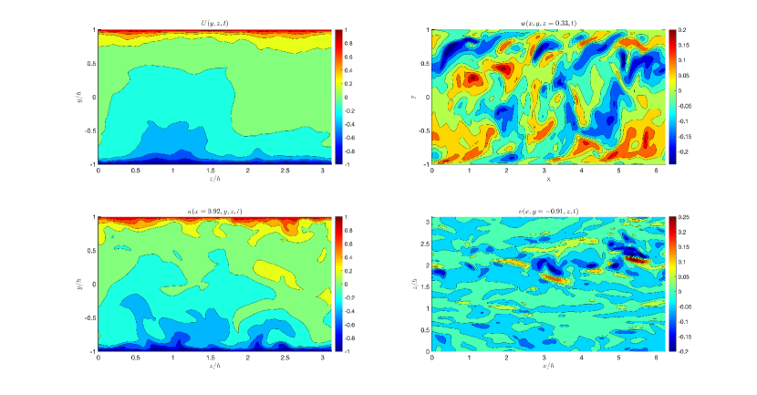
Figure 1: Instantaneous snapshots from the Couette test case C3 (cf. table 1) of the mean streamwise velocity $U(y,z,t)$ and velocity fields $(u,v,w)$ at $y-z$, $y-x$ and $z-x$ cross-sections on selected planes.

3 The integration scheme

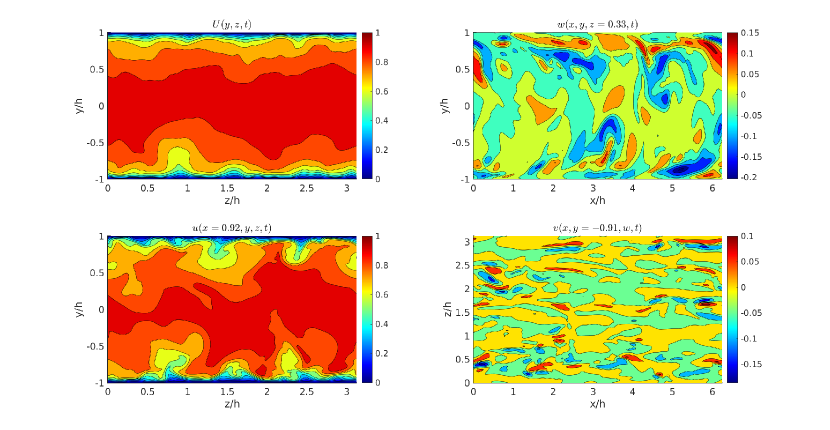
Figure 2: Same as Fig. 1 for the Poiseuille test case P3 (cf. table 1).

The time-stepping of this dynamical system was originally performed with a Crank-Nicolson / 2nd order Adams-Basforth integration scheme, while nowadays schemes with improved numerical stability are preferred, such as the Crank-Nicolson (CN)/ 3rd order Runge-Kutta (RK3) scheme which is implemented in this code. To advance the flow one $dt$ unit we have to perform 3 intermediate steps, based on the CN type of integration. At every intermediate step we can obtain evolution differential equations of $\Delta v$ and $\eta_{y}$ for each streamwise and spanwise wavenumber pairs, e.g.

$$\partial_{t}\Delta v^{(k^{\prime}_{x},k^{\prime}_{z})}= -(\partial_{xx}+\partial_{zz})(\mathbf{u}\cdot\mathbf{\nabla}v)^{(k^{\prime}_{x},k^{\prime}_{z})}+\partial_{yx}(\mathbf{u}\cdot\mathbf{\nabla}u)^{(k^{\prime}_{x},k^{\prime}_{z})}$$ (10)

$$+\partial_{yz}(\mathbf{u}\cdot\mathbf{\nabla}w)^{(k^{\prime}_{x},k^{\prime}_{z})}+\frac{1}{Re}\Delta\Delta v^{(k^{\prime}_{x},k^{\prime}_{z})},$$

Pseudo-spectral methods are employed to perform differentiations and inversions as matrix operations in the discrete space. Thus, derivatives in $y$ are replaced with Chebyshev differentiation matrices (’Functions/cheb.m’) [13] and derivatives in $x$ and $z$ can be prescribed with Toeplitz matrices [14]. For a more compact representation we will gather the nonlinear terms under a single variable, $F^{(k^{\prime}_{x},k^{\prime}_{z})}$. This reduces Eq. 10 to

$$\partial_{t}\Delta v^{(k^{\prime}_{x},k^{\prime}_{z})}=-F^{(k^{\prime}_{x},k^{\prime}_{z})}+\frac{1}{Re}\Delta\Delta v^{(k^{\prime}_{x},k^{\prime}_{z})},$$ (11)

that describes the forced biharmonic problem. Boundary conditions at the top and bottom walls $v_{\pm w}=\partial_{y}v_{\pm_{w}}=0$ are supplemented for the solution of the evolution equation, which are enforced in the 4-th order derivative (’Functions/cheb4bc.m’ [13]) resulting from multiplication of the two Laplacian operators, $\Delta\Delta=(\partial_{yy}-k^{\prime 2}_{x}-k^{\prime 2}_{z})^{2}=\partial_{yyyy}-2(k^{\prime 2}_{x}+k^{\prime 2}_{z})\partial_{yy}+(k^{\prime 2}_{x}+k^{\prime 2}_{z})^{2}$.

Evaluating the system of equations on a wavenumber pair basis reduces the inversion matrices to the square $N^{2}_{y}$ of the wall-normal grid points. Pseudo-spectral methods apply a 2/3rds de-aliasing filter in flow fields, where the highest 1/3 of the streamwise and spanwise harmonics are discarded [15]. The equations governing $v$ and $\eta$ can be then reformulated in compact sparse matrices with $k^{\prime}_{x}\otimes k^{\prime}_{z}\otimes R^{N^{2}_{y}}$, where the solver matrices for each ($k^{\prime}_{x},k^{\prime}_{z}$) pair are concatenated as blocks across the diagonal, which is executed as a single matrix multiplication operation. After reshaping $v$ and $\eta$ to single column vectors with $k^{\prime}_{x}\otimes k^{\prime}_{z}\otimes y$ Kronecker structure, we acquire their next step iteration from multiplication with these matrices.

It is straightforward to obtain the wall-normal dependence for the Fourier coefficients of $u$, $w$ with wavenumbers $(k^{\prime}_{x},k^{\prime}_{z})$ from the linear system comprised by the equations used to relate $u$ and $w$ with $\partial_{y}v$ (incompressibility) and $\eta$ (vorticity),

$$\begin{pmatrix}-ik^{\prime}_{x}\hat{u}&-ik^{\prime}_{z}\hat{w}\\ -ik^{\prime}_{z}\hat{u}&ik^{\prime}_{x}\hat{w}\end{pmatrix}=\begin{pmatrix}\partial_{y}\hat{v}\\ \hat{\eta}_{y}\end{pmatrix}$$ (12)

Solutions are found in the form

$$\hat{u}=\frac{-ik^{\prime}_{z}\hat{\eta}_{y}+ik^{\prime}_{x}\partial_{y}\hat{v}}{k^{\prime 2}_{x}+k^{\prime 2}_{z}}$$ (13)

$$\hat{w}=\frac{ik^{\prime}_{x}\hat{\eta}_{y}+ik^{\prime}_{z}\partial_{y}\hat{v}}{k^{\prime 2}_{x}+k^{\prime 2}_{z}}$$ (14)

which are also stored with a nesting hierarchy $k^{\prime}_{x}\otimes k^{\prime}_{z}\otimes y$ in the sparse matrices $\mathbf{kkm}$ and $\mathbf{llm}$, with the elements $\frac{ik^{\prime}_{x}}{k^{\prime 2}_{x}+k^{\prime 2}_{z}}$ and $\frac{ik^{\prime}_{z}}{k^{\prime 2}_{x}+k^{\prime 2}_{z}}$ filling the diagonal.

Lastly, the mean profiles $U_{00}$ and $W_{00}$ are evaluated separately. With $U_{00}(y)$ and $W_{00}(y)$ we can determine fully the $u$ and $w$ components of the velocity fields and thus acquire the complete solution for the next intermediate iteration or time-step.

3.1 The nonlinear term CN / RK3 scheme

As part of the semi-implicit Crank-Nicolson time-step, the nonlinear terms are approximated over at 3 half-steps. To advance the solution one $dt$ unit of time the set of equations will be progressively solved for 1 intermediate $dt/2$ interval and one intermediate $dt$ interval before the full $dt$ interval each time-step. A different approximation of all the nonlinear terms (last term in each of the equations (16-19)) is employed at each intermediate time-step. For Poiseuille flow, the pressure $\gamma(t)$ enforcing constant mass flux in Eq. 6 is also updated at each step. Employing the Crank-Nicolson time-stepping, we transform (11) to a difference equation at the initial time $t$ and its’ half/full time-step succession $t+hdt$,

$$\frac{v^{(k^{\prime}_{x},k^{\prime}_{z})}_{t+hdt}-v^{(k^{\prime}_{x},k^{\prime}_{z})}_{t}}{hdt}=-\Delta^{-1}F^{(k^{\prime}_{x},k^{\prime}_{z})}_{t}+\frac{1}{Re}\Delta^{-1}\left[\Delta\Delta\frac{v^{(k^{\prime}_{x},k^{\prime}_{z})}_{t+hdt}+v^{(k^{\prime}_{x},k^{\prime}_{z})}_{t}}{2}\right].$$ (15)

where the boundary condition of $v$ at the wall is utilized to invert $\Delta v$. As an example, $F^{(k^{\prime}_{x},k^{\prime}_{z})}_{t}$ will be evaluated at the first intermediate steps as $F^{0,(k^{\prime}_{x},k^{\prime}_{z})}_{t}$ and $h=1/2$, at the second intermediate step as $2F^{1,(k^{\prime}_{x},k^{\prime}_{z})}_{t}-F^{0,(k^{\prime}_{x},k^{\prime}_{z})}_{t}$ and $h=1$, before evaluating the final step with $(F^{0,(k^{\prime}_{x},k^{\prime}_{z})}_{t}+4F^{1,(k^{\prime}_{x},k^{\prime}_{z})}_{t}+F^{2,(k^{\prime}_{x},k^{\prime}_{z})}_{t})/6$ and $h=1$. The i superscript of $F^{i,(k^{\prime}_{x},k^{\prime}_{z})}_{t}$ indicates from which iteration of the velocity field they are being calculated, where $i=0$ denotes the actual velocity field at $t$. Notice that although the forcing terms are updated at each intermediate step, the initial state remains always the state at $t$.

The $F$ term contains all nonlinear terms and derivatives. It is important to replace the for-loops that could be employed to perform the derivations with matrix operations on the velocity variables. This is achieved using permutations (see the exact implementations in ”$Functions/{difX,difY,difZ}\_F.m$”) which transpose the coordinate where the differentiation matrix operates to the first dimension of the matrix, and restore the original order after the operation is complete. The point by point multiplications that occur in the $\mathbf{u}\cdot\mathbf{\nabla}u_{i}$ terms also benefit from GPU calculations, although to a lesser extend compared to the fft and the solution steps.

3.2 Solution with precalculated inverse matrices

We are now tasked with allocating separately the unknown and known quantities, which result in a linear system for $v^{(k^{\prime}_{x},k^{\prime}_{z})}_{t+hdt}$,

$$\left[I-hdt\frac{1}{2Re}\Delta^{-1}\Delta\Delta\right]v^{(k^{\prime}_{x},k^{\prime}_{z})}_{t+hdt}=\left[I+hdt\frac{1}{2Re}\Delta^{-1}\Delta\Delta\right]v^{(k^{\prime}_{x},k^{\prime}_{z})}_{t}$$

$$-hdt\Delta^{-1}F^{(k^{\prime}_{x},k^{\prime}_{z})}_{t},$$ (16)

$$\left[I-hdt\frac{1}{2Re}\Delta\right]\eta_{y,t+hdt}^{(k^{\prime}_{x},k^{\prime}_{z})}=\left[I+hdt\frac{1}{2Re}\Delta\right]\eta_{y,t}^{(k^{\prime}_{x},k^{\prime}_{z})}$$

$$-hdtG^{(k^{\prime}_{x},k^{\prime}_{z})}_{t},$$ (17)

$$\left[I-hdt\frac{1}{2Re}\partial_{yy}\right]U_{00,t+hdt}=\left[I+hdt\frac{1}{2Re}\partial_{yy}\right]U_{00,t}$$

$$-(f_{+}(U_{+w})+f_{-}(U_{-w}))-hdt\gamma(t)-hdt\partial_{y}\left[uv\right]_{t},$$ (18)

$$\left[I-hdt\frac{1}{2Re}\partial_{yy}\right]W_{00,t+hdt}=\left[I+hdt\frac{1}{2Re}\partial_{yy}\right]W_{00,t}$$

$$-hdt\partial_{y}\left[wv\right]_{t},$$ (19)

These difference equations are now in the form Ax = b, with x the unknown variable at time $t+hdt$ and b the rhs of each equation. It can be seen that the A matrices are constant for each $h$ and thus it is significantly faster to precalculate their inverses and store them. Following the ideas of preconditioning [9], since there are also constant matrices in the right hand side of the difference equations, it will be economical to perform the multiplication of the inverses with the constant matrices and eventually calculate only the results of matrix and vector multiplications. Special care has to be applied to the $U_{00}$ equation, when the boundary conditions are non-zero (Couette). We then have to separate the first and last column of $\left[I-hdt\frac{1}{2Re}\partial_{yy}\right]$, which multiply the boundary condition values at the top and bottom walls respectively, and move them to the right hand side with the terms to be inverted. In the other 3 cases the inversion matrix is evaluated with zero boundary conditions. After clarifying the boundary conditions, we invert the A matrices in the lhs excluding the boundary points, i.e. the inversion is performed on the matrix $[I-hdt\cdots]_{(2:M_{y}-1),(2:M_{y}-1)}$

4 Evaluation of the numerical code

Table 1: Simulation statistics of Couette (C2,C3,C4) and Poiseuille (P2,P3) test cases. Dimensions of the channels in wall units are indicated by $[L_{x}^{+},L_{y}^{+},L_{z}^{+}]$. $R_{\tau}=hu_{\tau}/\nu$ is the friction velocity Reynolds number according to $u_{\tau}$. The average spacing in $x$ and $z$ for the resolutions of simulations (cf. table 2) are denoted as $\Delta x^{+},~{}\Delta z^{+}$. The averaging time, $Tu_{t}/h$, is also reported.

Abbreviation	$[L^{+}_{x}\;\;,\;L^{+}_{y},\;\;L^{+}_{z}]$	$R_{\tau}$	$Tu_{\tau}/h$	$\Delta x^{+}$	$\Delta z^{+}$
C2	$[1073.8\;,341.8,\;536.9]$	$170.9$	$267.7$	$15.1$	$7.6$
C3	$[1076.3\;,342.6,\;538.2]$	$171.3$	$262.6$	$11.3$	$5.7$
C4	$[2145.1\;,341.4,\;1072.5]$	$170.7$	$273.1$	$20.8$	$10.4$
P2	$[1157.4\;,368.4,\;578.7]$	$184.2$	$221.0$	$16.3$	$8.2$
P3	$[1150.5\;,366.2,\;575.2]$	$183.1$	$276.0$	$12.1$	$6.1$

As validation for our code we collect one point statistics of the solution velocity fields. These are the time-averaged streamwise- and spanwise-mean velocity profile $U(y)$, the rms profile of the velocity fluctuations from the mean profile $(u^{\prime},v^{\prime},w^{\prime})$ and the tangential Reynolds stress $u^{\prime}v^{\prime}$. For the statistics we will run extensive DNSs using the GPU option of the code. Transition from CPU to GPU computation is implemented by the simple transfer of the appropriate variables to the GPU with the MATLAB command gpuArray. The well-resolved cases $(C3,P3)$ require approximately 2 days to complete over 250 $Tu_{\tau}/h$ units of time. We can compare the agreement of our statistics with the statistics of [16] (for plane Couette flow) and [17] (for plane Poiseuille flow). This comparison is shown for the cases of table 1 in Figs. 3 and 4.

It is evident that both the mean profile statistics and the velocity fluctuation rmss agree considerably with the benchmark $Re=3000$ case presented by [16] given that their case was calculated in a bigger domain. We can verify that statistics away from the wall converge to those of [16] by running the low resolution C4 in a box with periodic dimensions $[L_{x},L_{z}]=[4\pi,2\pi]$. Similar agreement was found when we compared the Poiseuille mean profile and fluctuation statistics with the benchmark of [17]. Instances of the streamwise-mean $U$ velocity field show the characteristic streaks rising from the walls in both flow configurations (Figs. 1a and 2a)

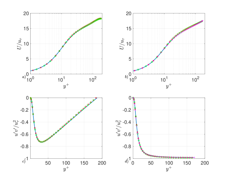
Figure 3: (a,c) Comparison of P2 (red squares) and P3 (green circles) with the statistics of the mean velocity profile $U$ (a) and the tangential shear stress (c) [17](solid blue lines). (b,d) Comparison of C2 (red squares), C3 (green circles) and C4 (purple crosses) with the statistics of the mean velocity profile $U$ (b) and the tangential shear stress (d) of [16] (solid blue lines). The results from our code show good agreement in both cases.

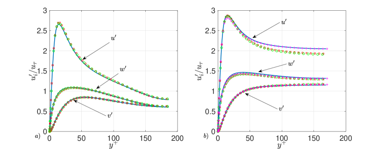
Figure 4: The rms profiles from a) [17] and b) [16] ( solid blue lines) of the streamwise ($u^{\prime}/u_{\tau}$), wall-normal ($v^{\prime}/u_{\tau}$), spanwise ($w^{\prime}/u_{\tau}$) velocity fluctuations from the mean profile $U$.These statistics agree reasonably well near the wall, whereas a deviation is noted in b) for the $u^{\prime},w^{\prime}$ profiles since the domain of [16] is considerably larger. This deviation further away from the wall is indeed seen to reduce for the coarse C4 case in a larger domain.

4.1 Comparisons with the MATLAB DNSLab solver

Table 2: Simulation parameters of C1-C4 and P1-P3. The channel size in the streamwise, wall-normal and spanwise directions is $[L_{x},L_{y},L_{z}]/h=[2\pi,2,\pi]$ in all cases except C4 where $[L_{x},L_{y},L_{z}]/h=[4\pi,2,2\pi]$, with $h$ being the channel half-width. $M_{x}$, $M_{z}$ are the number of points for the equally-distanced grid in the streamwise and spanwise direction and $M_{y}$ are the number of points on a Chebyshev grid, including the 2 points at the walls. $N_{x}$, $N_{z}$ are the number of ($\pm$) Fourier components after dealiasing and $N_{y}=M_{y}-2$. The average execution time (on CPU or GPU) per time-step over a simulation with 3000 time-steps is denoted as $\bar{T}^{CPU/GPU}_{dt}$.

Abbreviation	$[M_{x}\times M_{z}\times M_{y}]$	$N_{x}\times N_{z}\times N_{y}$	$N$	$\bar{T}^{CPU}_{dt}$	$\bar{T}^{GPU}_{dt}$
C1	$[72\;,72,\;63]$	$47\times 47\times 61$	$134749$	$0.1620$	$0.0606$
P1	$[72\;,72,\;63]$	$47\times 47\times 61$	$134749$	$0.1519$	$0.0624$
C2	$[108\;,108,\;73]$	$71\times 71\times 71$	$357911$	$0.5129$	$0.1308$
P2	$[108\;,108,\;73]$	$71\times 71\times 71$	$357911$	$0.4992$	$0.1366$
C3	$[144\;,144,\;83]$	$95\times 95\times 81$	$731025$	$1.1358$	$0.2821$
P3	$[144\;,144,\;83]$	$95\times 95\times 81$	$731025$	$1.1536$	$0.2922$
C4	$[156\;,156,\;83]$	$103\times 103\times 81$	$859329$	$1.4349$	$0.3390$

Table 3: Simulation parameters for VK cases. The channel size in the streamwise, wall-normal and spanwise directions is $[L_{x},L_{y},L_{z}]/h=[2\pi,2,\pi]$, where $h$ is the half-width. The number of points for the finite difference grid in the streamwise, spanwise and wall-normal directions are $N_{x}$, $N_{z}$ and $N_{y}$ (excluding the 2 points at the top and bottom wall). The average CPU execution time per time-step over a simulation with 3000 time-steps is denoted as $\bar{T}_{dt}$.

Abbreviation	$N_{x}\times N_{z}\times N_{y}$	$N$	$\bar{T}^{CPU}_{dt}$
VK1	$48\times 48\times 48$	$110592$	$0.2335$
VK2	$60\times 60\times 60$	$216000$	$0.5505$
VK3	$72\times 72\times 72$	$373248$	$1.2808$
VK4	$84\times 84\times 84$	$592704$	$2.5256$

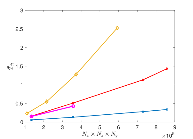
Figure 5: Average execution time $\bar{T}_{dt}$ required to advance the flow one time-step $dt$ as a function of resolved grid size. $\bar{T}_{dt}$ increases approximately as a linear function of the number of resolved grid points for the GPU cases (blue line), while the CPU (red line) moves away from this trend at the final point. We compare these with the $\bar{T}_{dt}$ from a series of simulations with the DNSLab suite [4] (mustard diamond) run at the same CPU. Finally, the purple circles are the C1-C2 cases run at a low-end GTX 1050 Ti GPU, which is still marginally faster than the respective cases run on the CPU.

The base study for comparison will be the DNSlab program suite developed by [4] for MATLAB and specifically their 3D Navier-Stokes solver. There a plane Poiseuille channel was simulated in a $[L_{x}\times L_{y}\times L_{z}]=[2\pi\times 2\times\pi]$ finite difference grid at friction Reynolds number $180$. A relatively coarse grid of $72^{3}$ points was employed (without including the 2 points at the walls), which demonstated the potential of MATLAB to run simulations of turbulence. Development of our Navier-Stokes solver was also started on a finite difference grid, which was eventually revised to the current version with a Chebyshev grid that enhances resolution near the walls and a programming structure that is more suitable for GPU calculation.

We will initially compare the case presented by [4](VK3) with the C2 case computed by the present DNS code. Since we employ the 2/3rds rule, we use an increased number of points in $x$ and $z$, which after dealiasing result in a marginally smaller but comparable number of grid points (373.2k for VK3, 357.9k for C2) . Crucially though, for the spectral methods one half of the harmonic pairs are complex conjugate to the other half and therefore we only need to tackle matrices with half the number of elements in each dimension, i.e with size one quarter of the VK3 case. The matrices in our code however are significantly denser due to the Chebyshev differentiation, which is reflected in the greater memory space occupied by the matrices we utilize. We expect the memory requirements to scale as $9\cdot 16[(Nx/2)\cdot Nz\cdot Ny^{2}]$ bytes, since 9 sparse matrices with this structure are loaded to the GPU memory, each element occupies 16 bytes due to itself and its indices, and only the sub-matrices with $N^{2}_{y}$ elements are dense.

Solutions for the two cases were calculated using an i9-9900k CPU for 3000 time steps. The timing benchmarks between the two cases show that C2 completes a time-step about 2.5 times faster than VK3 on average. This already is a considerable improvement given the identical conditions of the test. The tradeoff paid for this speed boost is found in the respective memory utilization, where VK3 uses about  500 MB, whereas C2 occupies about  2500 MB. Additional cases are tested to document the dependence of $\bar{T}_{dt}$ as the number of grid points changes. For the DNSLab cases we observe an increase in $\bar{T}_{dt}$ that is steeper than linear (Fig.5). On the other hand, cases C1-C4 run on GPU exhibit a linear behaviour, suggesting a better scaling for our code across cases with sizes that fit in the GPU memory.

The costly part of the time integration in VK is the pressure correction. In the 3000 time-steps, their code spends approximately $80\%$ of the time on the correction and projection stages, with the majority of it owned to the bicgstab.m function solving the pressure Laplacian. For our code, the rkstep.m is the most time-consuming, particularly the multiplication of the precalculated matrices with the current $v$ and $\eta$ and the respective advection terms to obtain their new values.

4.2 Timing of CPU and GPU runs in the current code

The greatest boost accomplished when comparing GPU with CPU execution on our code is seen in the fft2 calculations. There, total time spent to perform the ffts is reduced to the 1/6th of that required on the CPU. An improvement of $3.5\times$ is noted on the rkstep where the matrix multiplications responsible for inverting and updating the field to the next intermediate step are executed. Finally, a nearly $2.5\times$ reduction is seen in the evaluation of the nonlinear advection term, where matrix and point by point multiplications occur. These last operations are also more computationally intensive since here the full, rather than the dealiased, degrees of freedom come into play. To investigate a possible reduction of execution time in the VK code versions of the bicgstab function should be ported efficiently to GPU, however we are not aware of any such version available for MATLAB at the time, while the DNSLABIB uses different methods to obtain the pressure.

5 Conclusions

We have presented a Navier-Stokes solver which utilizes the built-in MATLAB vectorization to complete DNSs spanning  250 eddy turn-over times in a time-frame between tens of hours to a couple of days given the hardware at our disposal and the resolution of the computational grid. This code improves over the DNSLab time-step performance by $\approx 2.5\times$ when both codes use exclusively the CPU, with an acceleration of up to $\approx 9\times$ when we utilize the GPU acceleration available in our code. We also demonstrated the accuracy of simulation statistics for the two main channel options available in the code, the plane Couette and plane Poiseuille flows, at a friction Reynolds number of $\approx 170-180$.

The hardware used for these simulations would be considered enthusiast grade at its’ release time, while the GTX 1050 Ti is more of an entry level GPU. Although the theoretically available peak double precision GFLOPs of the TITAN Z Black are $\approx 1700$ (for the single module that is used), comparison with a GTX 1050 Ti (with $\approx 66$ available GLOPS) shows only an improvement of $3\times$ in performance instead of the expected $25\times$. This suggests that there may even exist potential for significant improvement in the current code. Finally, another factor that should favor even more reduced execution times is utilization of newer GPU hardware, since today GPUs with considerably higher GFLOPs than the TITAN Z are available.

Acknowledgements

M.-A. Nikolaidis gratefully acknowledges the partial support by the Hellenic Foundation for Research and Innovation (HFRI) and the General Secretariat for Research and Technology (GSRT), under the HFRI PhD Fellowship grant 1718/ 14518. The author wishes to thank Petros J. Ioannou, Brian F. Farrell and Navid C. Constantinou for fruitful discussions during the development of this code and opportunities to use it. Additional thanks are extended to J. Jiménez and A. Lozano-Durán for introducing the author to the MPI DNS code developed by the Fluid Dynamics group at UPM.

Declaration of Competing Interest

The author declares that he has no known competing financial interests or personal relationships that could have appered to influence the work reported in this paper.

References

- [1] D. Jacobsen, J. Thibault, I. Senocak, An MPI-CUDA Implementation for Massively Parallel Incompressible Flow Computations on Multi-GPU Clusters. arXiv:https://arc.aiaa.org/doi/pdf/10.2514/6.2010-522, doi:10.2514/6.2010-522.
- [2] A. Khajeh-Saeed, J. B. Perot, Direct numerical simulation of turbulence using GPU accelerated supercomputers, Journal of Computational Physics 235 (2013) 241–257. doi:https://doi.org/10.1016/j.jcp.2012.10.050.
- [3] A. Vela-Martín, M. P. Encinar, A. García-Gutiérrez, J. Jiménez, A low-storage method consistent with second-order statistics for time-resolved databases of turbulent channel flow up to , Journal of Computational Science 56 (2021) 101476. doi:https://doi.org/10.1016/j.jocs.2021.101476.
- [4] V. Vuorinen, K. Keskinen, DNSLab: A gateway to turbulent flow simulation in Matlab, Computer Physics Communications 203 (2016) 278–289. doi:https://doi.org/10.1016/j.cpc.2016.02.023.
- [5] M. Korhonen, A. Laitinen, G. E. Isitman, L. Jimenez, V. Vuorinen, A GPU-accelerated computational fluid dynamics solver for assessing shear-driven indoor airflow and virus transmission by scale-resolved simulations(arXiv:2204.02107) (2022).
- [6] D. Gottlieb, S. A. Orszag, Numerical Analysis of Spectral Methods, Society for Industrial and Applied Mathematics, 1977. arXiv:https://epubs.siam.org/doi/pdf/10.1137/1.9781611970425, doi:10.1137/1.9781611970425.
- [7] S. A. Orszag, Comparison of pseudospectral and spectral approximation, Studies in Applied Mathematics 51 (3) (1972) 253–259. arXiv:https://onlinelibrary.wiley.com/doi/pdf/10.1002/sapm1972513253, doi:https://doi.org/10.1002/sapm1972513253.
- [8] C. Lanczos, Applied Analysis, Prentice Hall, 1956.
- [9] M. Hussaini, D. Kopriva, A. Patera, Spectral collocation methods, Applied Numerical Mathematics 5 (3) (1989) 177–208. doi:https://doi.org/10.1016/0168-9274(89)90033-0.
- [10] B. Fornberg, A Practical Guide to Pseudospectral Methods, Cambridge University Press, 1996.
- [11] P. R. Spalart, R. D. Moser, M. M. Rogers, Spectral methods for the navier-stokes equations with one infinite and two periodic directions, Journal of Computational Physics 96 (2) (1991) 297–324. doi:https://doi.org/10.1016/0021-9991(91)90238-G.
- [12] J. Kim, P. Moin, R. Moser, Turbulence statistics in fully developed channel flow at low Reynolds number, J. Fluid Mech. 177 (1987) 133–166. doi:10.1017/S0022112087000892.
- [13] J. A. C. Weideman, S. C. Reddy, A MATLAB differentiation matrix suite, ACM TOMS (2000).
- [14] L. N. Trefethen, Spectral Methods in MATLAB, SIAM, 2000.
- [15] S. A. Orszag, On the Elimination of Aliasing in Finite-Difference Schemes by Filtering High-Wavenumber Components, Journal of Atmospheric Sciences 28 (6) (1971) 1074 – 1074.
- [16] S. Pirozzoli, M. Bernardini, P. Orlandi, Turbulence statistics in Couette flow at high Reynolds number, Journal of Fluid Mechanics 758 (2014) 327–343. doi:10.1017/jfm.2014.529.
- [17] J. C. del Álamo, J. Jiménez, Spectra of the very large anisotropic scales in turbulent channels, Phys. Fluids 15 (2003) L41–L44. doi:10.1017/S002211200300733X.