Recovery of consistency in thermodynamics of regular black holes in Einstein’s gravity coupled with nonlinear electrodynamics

Yang Guo, Hao Xie, and Yan-Gang Miao

School of Physics, Nankai University, Tianjin 300071, China

As one of candidate theories in the construction of regular black holes, Einstein’s gravity coupled with nonlinear electrodynamics has been a topic of great concerns. Owing to the coupling between Einstein’s gravity and nonlinear electrodynamics, we need to reconsider the first law of thermodynamics, which will lead to a new thermodynamic phase space. In such a phase space, the equation of state accurately describes the complete phase transition process of regular black holes. The Maxwell equal area law strictly holds when the phase transition occurs, and the entropy obeys the Bekenstein-Hawking area formula, which is compatible with the situation in Einstein’s gravity.

1 Introduction

Regular black holes in Einstein’s gravity coupled with nonlinear electrodynamics (NLD) have been studied [1, 2, 3, 4] extensively in recent years, which is related closely to the singularity of spacetime. In Einstein’s gravity, the singularity theorem established by Hawking and Penrose [5] claims that it is an inevitable feature of the theory itself. However, it is generally accepted that such a singularity is unphysical on the classical level and should be served as an evidence that the general relativity (GR) requires modifications or generalizations to incorporating quantum theories. The nonlinear electrodynamics provides a crucial contribution to avoiding singularities of black holes, which allows us to construct [6, 7, 8, 9, 10, 11] regular black holes with a nonlinear electromagnetic source.

More recently, a remarkable progress has been made [12, 13, 14, 15, 16, 17, 18, 19] in the study of thermodynamics of regular black holes in Einstein’s gravity coupled with nonlinear electrodynamics. However, there exist some difficulties and challenges, for instance, the Maxwell equal area law is violated [20] during the process in the small-large phase transformation, and the entropy does not obey [21, 22, 23] the Bekenstein-Hawking area formula. After an in-depth review, we find that these difficulties and challenges are caused by a superficial application of the methodology developed [24, 25, 26] in Einstein’s gravity to the theory of Einstein’s gravity coupled with nonlinear electrodynamics. More precisely, the first law of black hole thermodynamics in Einstein’s gravity should be modified in the theory of Einstein’s gravity coupled with nonlinear electrodynamics. If not, the naive application would lead to an incorrect and incomplete phase space in which the equation of state could not accurately describe the phase transition of regular black holes. Consequently, the first law of thermodynamics should be reconsidered for regular black holes in the theory of Einstein’s gravity coupled with nonlinear electrodynamics.

After giving an improved first law of thermodynamics in terms of a covariant approach [27, 28], we can eliminate the inconsistency previously appeared in thermodynamics of regular black holes with the price of introducing a new thermodynamic phase space. In this new phase space, the Maxwell equal area law holds strictly, and the entropy obeys the Bekenstein-Hawking area formula, which is compatible with the situation in Einstein’s gravity. In addition, the phase transition behavior of regular black holes is completely described by the equation of state in the new phase space. We may say that our work provides a refined approach to thermodynamics of regular black holes in Einstein’s gravity coupled with nonlinear electrodynamics.

Our paper is organized as follows. In Sec. 2.1, we introduce the basics for Einstein’s gravity coupled with nonlinear electrodynamics. In Sec. 2.2, we derive the first law and Smarr formula in terms of a covariant approach for regular black holes in Einstein’s gravity coupled with nonlinear electrodynamics. Next, we demonstrate a general approach to thermodynamics of regular black holes in a new extended phase space in Einstein’s gravity coupled with nonlinear electrodynamics in Sec. 3.1, and then apply this approach to two specific regular black holes in Sec. 3.2 and Sec. 3.3, where Sec. 3.2 is devoted to the first law and the Bekenstein-Hawking area formula and Sec. 3.2 to a universal number at critical points. Finally, we summarize our results in Sec. 4.

2 Einstein’s gravity coupled with nonlinear electrodynamics

2.1 Nonlinear electrodynamics

The Einstein gravity coupled with nonlinear electrodynamics can be described by the action,

$$S=\frac{1}{16\pi}\int d^{4}x\sqrt{-g}\left[{R}-\mathcal{L}(F)\right],$$ (2.1)

where $R$ is scalar curvature, $F\equiv\frac{1}{4}F^{ab}F_{ab}$ is electromagnetic invariant, and $F_{ab}\equiv\partial_{a}A_{b}-\partial_{b}A_{a}$ is field strength with $A_{a}$ a vector potential. By varying the action with respect to $A_{a}$, one obtains the following equation,

$$\nabla_{a}G^{ab}=0,$$ (2.2)

where $G^{ab}$ is defined by

$$G^{ab}\equiv\frac{1}{2}\frac{\partial\mathcal{L}(F)}{\partial F_{ab}}=\frac{1}{4}\mathcal{L}^{\prime}(F)F^{ab},$$ (2.3)

and the prime denotes a derivative with respect to $F$. Then one gives the corresponding magnetic charge and electric charges, respectively,

$$Q_{m} = \frac{1}{4\pi}\int_{\partial\Sigma}F_{ab},$$ (2.4)

$$Q_{e} = \frac{1}{4\pi}\int_{\partial\Sigma}{{}^{*}}G_{ab},$$ (2.5)

where ^∗ is Hodge star operator given by

$${{}^{*}}G_{ab}=\frac{1}{2!}\epsilon_{abcd}G^{cd}.$$ (2.6)

In a stationary spacetime, there exists a timelike Killing vector field, $\xi^{a}$, with which the electric and magnetic fields can be expressed by

$$E_{a} = F_{ab}\xi^{b},$$ (2.7)

$$H_{a} = -{{}^{*}}G_{ab}\xi^{b}.$$ (2.8)

Considering the fact that the field strength, $F_{ab}$, is closed, one has

$$0=\xi^{c}\nabla_{[a}F_{bc]}=\frac{1}{6}\xi^{c}(\nabla_{a}F_{bc}+\nabla_{b}F_{ca}+\nabla_{c}F_{ab}-\nabla_{a}F_{cb}-\nabla_{b}F_{ac}-\nabla_{c}F_{ba}).$$ (2.9)

Along the Killing vector field, the Lie derivative reads

$$\mathscr{L}_{\xi}F_{ab}=\xi^{c}\nabla_{c}F_{ab}+F_{cb}\nabla_{a}\xi^{c}+F_{ac}\nabla_{b}\xi^{c}=0.$$ (2.10)

Substituting Eq. (2.9) into Eq. (2.10) and considering the anti-symmetry of $F_{ab}$, one derives the equation,

$$\xi^{c}\nabla_{a}F_{bc}-\xi^{c}\nabla_{b}F_{ac}+F_{bc}\nabla_{a}\xi^{c}-F_{ac}\nabla_{b}\xi^{c}=0,$$ (2.11)

which can be rewritten, if one utilizes the Leibniz law, as follows:

$$\frac{1}{2}\left\{\nabla_{a}(F_{bc}\xi^{c})-\nabla_{b}(F_{ac}\xi^{c})\right\}=\frac{1}{2}(\nabla_{a}E_{b}-\nabla_{b}E_{a})=\nabla_{[a}E_{b]}=\frac{1}{2}(\text{d}E)_{ab}=0,$$ (2.12)

where d is exterior derivative operator. The above relation shows that the electric field, $E_{a}$, is closed.

Utilizing the definition of exterior derivatives and Hodge duals, one gives

$$(\text{d}{{}^{*}}G)_{fgd}=\frac{3}{2}\nabla_{[f}\epsilon_{gd]ab}G^{ab}.$$ (2.13)

Contracting both sides of Eq. (2.13) with $\epsilon^{efgd}$, one further derives

$$\epsilon^{efgd}(\text{d}{{}^{*}}G)_{fgd}=\frac{3}{2}\epsilon^{efgd}\nabla_{[f}\epsilon_{gd]ab}G^{ab}=6\nabla_{f}G^{fe}.$$ (2.14)

Again contracting both sides of Eq. (2.14) with $\epsilon_{ecab}$ and using Eq. (2.2), one finally obtains

$$(\text{d}{{}^{*}}G)_{cab}=-\epsilon_{ecab}\nabla_{f}G^{fe}=0,$$ (2.15)

which shows that ${{}^{*}}G_{ab}$ is closed. As a result, the electric field, $E_{a}$, and magnetic field, $H_{a}$, can be expressed as the exterior derivatives of the scalar fields $\Phi$ and $\Psi$, respectively,

$$E_{a} = -\nabla_{a}\Phi,$$ (2.16)

$$H_{a} = -\nabla_{a}\Psi,$$ (2.17)

where $\Phi$ is electric potential and $\Psi$ magnetic potential.

2.2 First law and Smarr formula for regular black holes

We investigate a model with generality in Einstein’s gravity coupled with nonlinear electrodynamics, where the Lagrangian density of nonlinear electrodynamics takes the form [11],

$$\mathcal{L}(\mathcal{F})=\frac{4\mu}{\alpha}\frac{(\alpha\mathcal{F})^{(\nu+3)/4}}{\left[1+(\alpha\mathcal{F})^{\nu/4}\right]^{(\mu+\nu)/\nu}},$$ (2.18)

$\mu$ and $\nu$ are dimensionless constants which characterize the nonlinear degree of electromagnetic fields, $\mathcal{F}$ is electromagnetic invariant, and $\alpha$ is constant parameter with the dimension of length squared. In this model, there existed some misinterpretations for mass parameters although such a model gave contributions to the study of regular black holes. In Ref. [11] the ADM mass was defined by

$$M_{\rm ADM}=M+\frac{q^{3}}{\alpha},$$ (2.19)

where $q$ was magnetic charge, and $M$ was interpreted improperly as the gravitational mass, i.e., $M=M_{g}$. Such a setup gives rise to an imperfect result that the corresponding regular black hole was non-singular only with a vanishing gravitational mass. We note that a regular black hole with a vanishing gravitational mass is acceptable mathematically but ill-defined physically due to lack of gravitational interaction. A reasonable interpretation for mass parameters suggests [29, 30] that the gravitational mass $M_{g}$ should equal the electromagnetically induced mass $M_{em}$,

$$M_{g}=M_{em}=\frac{q^{3}}{\alpha},$$ (2.20)

which allows the mass parameter of regular black holes to be well explained. In order to make regular black holes well-defined, that is, the mass parameter that appears in the Lagrangian density denotes ADM mass, we make the crucial transformations in Eq. (2.18),

$$\mathcal{F}\rightarrow\frac{2M}{q}F,\qquad\alpha\rightarrow\frac{q^{3}}{M},$$ (2.21)

and then change the Lagrangian density of nonlinear electrodynamics to the following form,

$$\mathcal{L}(F)=\frac{4\mu M\left(2Fq^{2}\right)^{(\nu+3)/4}}{q^{3}\left[1+\left(2Fq^{2}\right)^{\nu/4}\right]^{(\mu+\nu)/\nu}},$$ (2.22)

in which $M$ is exactly the ADM mass as we shall see. We can thus construct regular black holes, such as the Bardeen-like and Hayward-like ones, by varying $\mu$ and $\nu$. It is easy to check that Eq. (2.22) reduces to the Bardeen model [6] when $\mu=3$ and $\nu=2$, and to the Hayward model [31] when $\mu=\nu=3$. As a result, according to Eqs. (2.1) and (2.22), we deduce a general static and spherically symmetric solution in Einstein’s gravity coupled with nonlinear electrodynamics, where the corresponding shape function reads

$$f=1-\frac{2Mq^{3}r^{\mu-1}}{(r^{\nu}+q^{\nu})^{\mu/\nu}}.$$ (2.23)

One form of the first law was established [27] via a covariant approach in the framework of Einstein’s gravity coupled with nonlinear electrodynamics. However, the electromagnetic invariant $F$ was assumed [27] to be the only variable in the Lagrangian density of nonlinear electrodynamics, see Eq. (2.22), which leads to the limitation that this form of the first law holds for Born-Infeld black holes but not for Bardeen black holes. As is known, a correct first law should be universal, which means that it holds for any regular black hole solution from this framework. For the purpose to make this covariant approach valid for any regular black hole in Einstein’s gravity coupled with nonlinear electrodynamics, it was suggested [28] that all parameters in the Lagrangian density of nonlinear electrodynamics, including the electromagnetic invariant and other parameters such as charge and mass, must be treated as variables. As a result, the improved first law was written [28] as follows:

$$\delta M=\frac{\kappa}{8\pi}\delta A+\Phi\delta Q_{e}+\Psi\delta Q_{m}+\sum_{i}K_{i}\delta\beta_{i},$$ (2.24)

where $\beta_{i}$ denotes the parameters except the electromagnetic invariant, e.g. mass and charge, and $K_{i}$ is given by

$$K_{i}=\frac{1}{16\pi}\int_{\Sigma}\frac{\partial\mathcal{L}}{\partial\beta_{i}}\xi^{d}\epsilon_{dabc}.$$ (2.25)

Moreover, the field strength can be expressed [6] as

$$F_{ab}=q\sin\theta(\text{d}\theta)_{a}\wedge(\text{d}\phi)_{b},$$ (2.26)

and correspondingly the magnetic charge $Q_{m}$ appeared in Eq. (2.24) can be verified as $q$,

$$Q_{m}=\frac{1}{4\pi}\int_{\partial\Sigma}F_{ab}=q,$$ (2.27)

when Eqs. (2.4) and (2.26) are utilized.

Now we focus on the improved form of the first law, Eq. (2.24), and its corresponding Smarr formula for the general model depicted by Eqs. (2.1) and (2.22). At first, it is obvious that the electric potential, $\Phi$, vanishes because this model is irrelevant to electric charge. Then, we compute the magnetic field by using Eq. (2.8),

$$H_{a}=\frac{\mu M\left[\nu+3-(\mu-3)q^{\nu}r^{-\nu}\right]q^{\nu-1}r^{1-\nu}}{2r^{2}\left(1+q^{\nu}r^{-\nu}\right)^{\mu/\nu+2}}(\text{d}r)_{a},$$ (2.28)

and consequently obtain the magnetic potential on the horizon by substituting the above equation into Eq. (2.17),

$$\Psi=\frac{M\left\{\mu q^{\nu}r_{+}^{-\nu}+3\left(1+q^{\nu}r_{+}^{-\nu}\right)\left[\left(1+q^{\nu}r_{+}^{-\nu}\right)^{\mu/\nu}-1\right]\right\}}{2q\left(1+q^{\nu}r_{+}^{-\nu}\right)^{(\mu+\nu)/\nu}}.$$ (2.29)

Next, considering that $\beta_{i}$ corresponds to $M$ and $q$ in the model described by Eqs. (2.1) and (2.22), we derive the corresponding $K_{i}$ by using Eq. (2.25),

$$K_{q} = \frac{1}{16\pi}\int_{\Sigma}\frac{\partial\mathcal{L}}{\partial q}\xi^{d}\epsilon_{dabc}=\frac{Mr_{+}^{\mu}\left[3-3\left(q^{\nu}r_{+}^{-\nu}+1\right)^{\mu/\nu}+\mu q^{\nu}(r_{+}^{\nu}+q^{\nu})^{-1}\right]}{2q\left(r_{+}^{\nu}+q^{\nu}\right)^{\mu/\nu}},$$ (2.30)

$$K_{M} = \frac{1}{16\pi}\int_{\Sigma}\frac{\partial\mathcal{L}}{\partial M}\xi^{d}\epsilon_{dabc}=1-\frac{r_{+}^{\mu}}{\left(r_{+}^{\nu}+q^{\nu}\right)^{\mu/\nu}}.$$ (2.31)

At this stage, we deduce the first law of mechanics for regular black holes in Einstein’s gravity coupled with nonlinear electrodynamics,

$$\delta M=\frac{\kappa}{8\pi}\delta A+\Psi\delta q+K_{q}\delta q+K_{M}\delta M,$$ (2.32)

and the corresponding Smarr formula,

$$M=\frac{\kappa}{4\pi}A+\Psi q+K_{q}q+K_{M}M.$$ (2.33)

By varying $\mu$ and $\nu$, we can check that the Bardeen and Hayward black holes satisfy the above first law and Smarr formula. Here we note that the mass parameter $M$ that appears in Eq. (2.22) is exactly the ADM mass, which makes the mass parameter well-explained for regular black holes.

3 Thermodynamics in a new extended phase space

3.1 Thermodynamics in a new extended phase space for regular black holes in Einstein’s gravity coupled with nonlinear electrodynamics

In Einstein’s gravity, the thermodynamics of black holes has been studied [32, 33, 34, 35] extensively and many effective methodologies have been developed [24, 25, 26]. However, in Einstein’s gravity coupled with nonlinear electrodynamics, the study of thermodynamics of regular black holes has presented difficulties and problems, such as inconsistencies [20] between the Maxwell equal area law and the Gibbs free energy during the phase transition of small-large regular black holes, and deviations [21] in calculations of thermodynamic quantities. We point out that one cannot simply generalize the methodology developed in Einstein’s gravity to Einstein’s gravity coupled with nonlinear electrodynamics for the study of regular black hole thermodynamics. In particular, we must reconsider thermodynamics based on an improved first law we are going to figure out. In this subsection, we provide the fundamental approach to investigate thermodynamics of regular black holes in Einstein’s gravity coupled with nonlinear electrodynamics. In a new extended phase space where the cosmological constant is identified as pressure, $P=-\Lambda/(8\pi)$, we write an improved first law of thermodynamics from Eq. (2.32) as a compact form,

$$dM=T^{\prime}dS+\Psi^{\prime}dq+V^{\prime}dP,$$ (3.1)

where

$$T^{\prime}=\frac{T}{1-K_{M}},\qquad\Psi^{\prime}=\frac{\Psi+K_{q}}{1-K_{M}},\qquad V^{\prime}=\frac{V}{1-K_{M}}.$$ (3.2)

We note that the new extended phase space consists of ($T^{\prime}$, $S$), ($\Psi^{\prime}$, $q$), and ($P$, $V^{\prime}$) rather than ($T$, $S$), ($\Psi$, $q$), and ($P$, $V$). In other words, it is composed of ($T^{\prime}$, $\Psi^{\prime}$, $P$, $S$, $q$, $V^{\prime}$). As we shall see in the next subsection, it is crucial to fix ($T^{\prime}$, $\Psi^{\prime}$, $V^{\prime}$) for addressing those difficulties mentioned above in thermodynamics of regular black holes in Einstein’s gravity coupled with nonlinear electrodynamics.

In thermodynamics, Gibbs free energy is equal to the maximum work that a thermodynamically closed system performs at constant temperature and pressure. Therefore, we can define the new Gibbs free energy by using the new temperature $T^{\prime}$ instead of the Hawking temperature $T$,

$$G^{\prime}=M-T^{\prime}S,$$ (3.3)

in order to distinguish from $G=M-TS$. We emphasize that the newly defined Gibbs free energy is distinct from the off-shell generalized free energy defined [36, 37, 38, 39] by an ensemble temperature. The reason is that an ensemble temperature is an external adjustable parameter and it is independent of black hole parameters. Here $T^{\prime}$ is correlated highly with the Hawking temperature and depends on black hole parameters. More importantly, it satisfies the equation of state. Thus the new Gibbs free energy defined in Eq. (3.3) is on-shell. Using Eqs. (3.1) and (3.3), we obtain the differential form of Gibbs free energy,

$$dG^{\prime}=-SdT^{\prime}+\Psi^{\prime}dq+V^{\prime}dP.$$ (3.4)

In order to clarify the relation between phase transitions and the Maxwell equal area law, we plot the oscillatory $(P,V^{\prime})$ behavior in Fig. 1, and the relations of $(G^{\prime},T^{\prime})$ and $(G^{\prime},P)$ in Fig. 2. When a regular black hole transforms from state A to state ${\rm A^{\prime}}$, the two states have the same Gibbs free energy. Therefore, by integrating Eq. (3.4) at constant $T^{\prime}$ and $q$, we have

$$\oint V^{\prime}dP=0,$$ (3.5)

where the integral is over the closed path: A $\rightarrow$ B $\rightarrow$ C $\rightarrow$ D $\rightarrow$ ${\rm A^{\prime}}$ in Fig. 1, where state A to state ${\rm A^{\prime}}$ have the same pressure. Thus, we have the equal area law,

$$\rm Area(ABC)=Area(A^{\prime}DC).$$ (3.6)

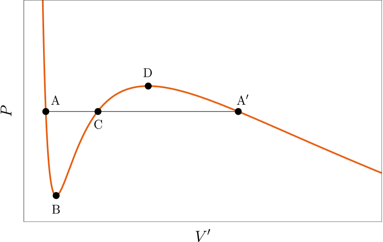
(a) $P-V^{\prime}$ plane

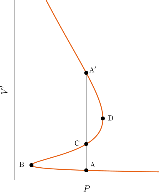
(b) $V^{\prime}-P$ plane

Figure 1: The oscillatory behavior of regular black holes in Einstein’s gravity coupled with nonlinear electrodynamics.

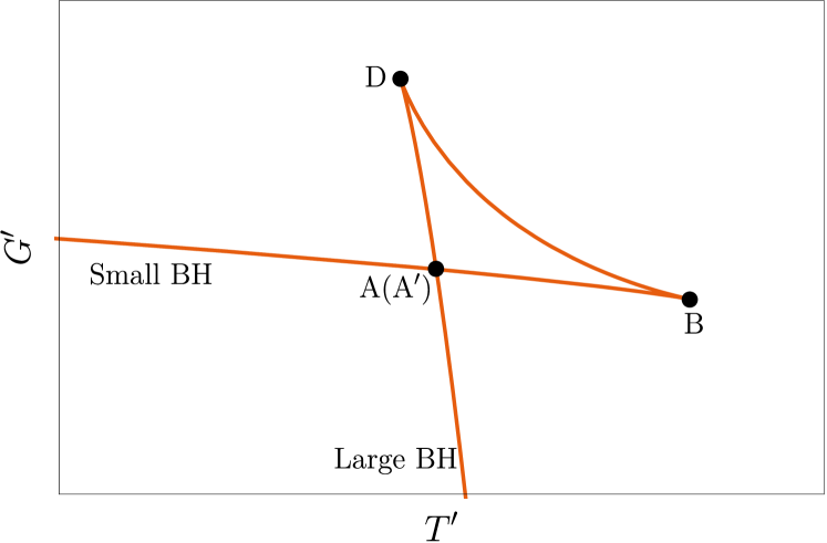
(a) $G^{\prime}-T^{\prime}$ plane

(b) $G^{\prime}-P$ plane

Figure 2: The Gibbs free energy $G^{\prime}$ with respect to $T^{\prime}$ and $P$ for regular black holes in Einstein’s gravity coupled with nonlinear electrodynamics.

The presence of oscillatory behaviors on the $P-V^{\prime}$ plane characterizes the phase transitions occurring in regular black holes, and so does the presence of swallow tail behaviors on the $G^{\prime}-T^{\prime}$ and $G^{\prime}-P$ planes. The oscillatory behavior in Fig. 1 appears only at the temperature below the critical value $T^{\prime}_{c}$, which shows that the Maxwell equal area law holds. When $T^{\prime}$ increases gradually, the area(ABC) or ${\rm area(A^{\prime}DC)}$ will become small. Meanwhile, the area of swallow tails in Fig. 2 also becomes small. Once the temperature or pressure reaches the critical value, $T^{\prime}_{c}$ or $P_{c}$, the oscillatory behavior in Fig. 1 and the swallow tail behavior in Fig. 2 disappear. We plot the critical behavior of $G^{\prime}$ in Figs. 3(a) and 3(b). At this critical point, the first-order phase transition turns into a second-order one because the entropy and volume are finite and continuous. We write the entropy and volume,

$$S = -\left(\frac{\partial G^{\prime}}{\partial T^{\prime}}\right)_{P_{c},q},$$ (3.7)

$$V^{\prime} = \left(\frac{\partial G^{\prime}}{\partial P}\right)_{T_{c}^{\prime},q},$$ (3.8)

and see their finiteness and continuity from the two sides of $T_{c}^{\prime}$ and of $P_{c}$ in Figs. 3(c) and 3(d), respectively. At this second-order phase transition point, the two phases stay at the same thermodynamic state, meaning no coexistence of small and large regular black holes. Nonetheless, the second-order derivatives of $G^{\prime}$ with respect to $P$ and $T^{\prime}$ are infinite at this point,

$$\left(\frac{\partial^{2}G^{\prime}}{\partial P^{2}}\right)_{T^{\prime}_{c},q} = \left(\frac{\partial V^{\prime}}{\partial P}\right)_{T^{\prime}_{c},q}\rightarrow-\infty,$$ (3.9)

$$\left(\frac{\partial^{2}G^{\prime}}{\partial T^{\prime 2}}\right)_{P_{c},q} = -\left(\frac{\partial S}{\partial T^{\prime}}\right)_{P_{c},q}\rightarrow-\infty.$$ (3.10)

Therefore, the heat capacity of regular black holes,

$$C_{p}=T^{\prime}\left(\frac{\partial S}{\partial T^{\prime}}\right)_{P_{c},q}=-T^{\prime}\left(\frac{\partial^{2}G^{\prime}}{\partial T^{\prime 2}}\right)_{P_{c},q}\rightarrow+\infty,$$ (3.11)

exhibits an infinite peak at $T_{c}^{\prime}$ or $P_{c}$ because it corresponds to the second-order derivative of Gibbs free energy, which is shown in Figs. 3(e) and 3(f).

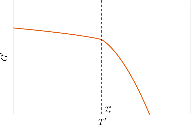
(a)

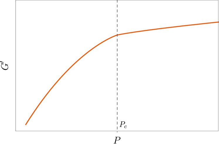
(b)

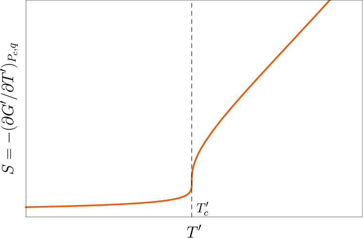
(c)

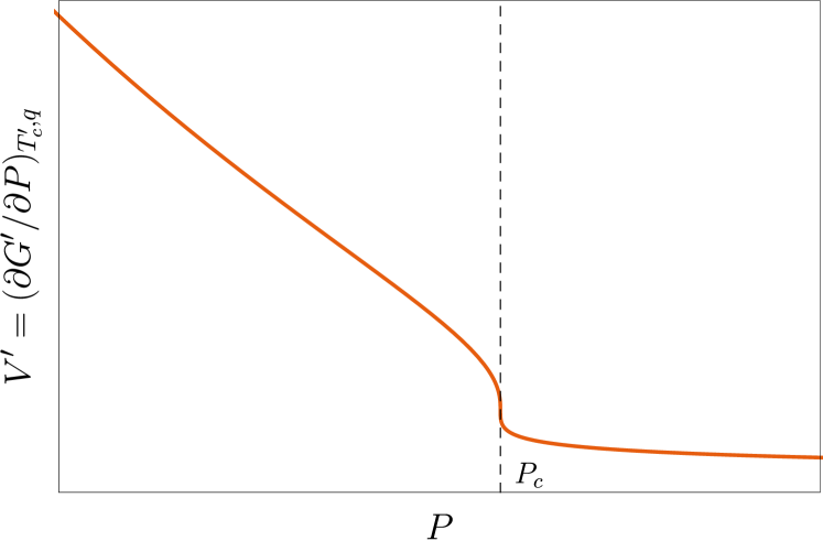
(d)

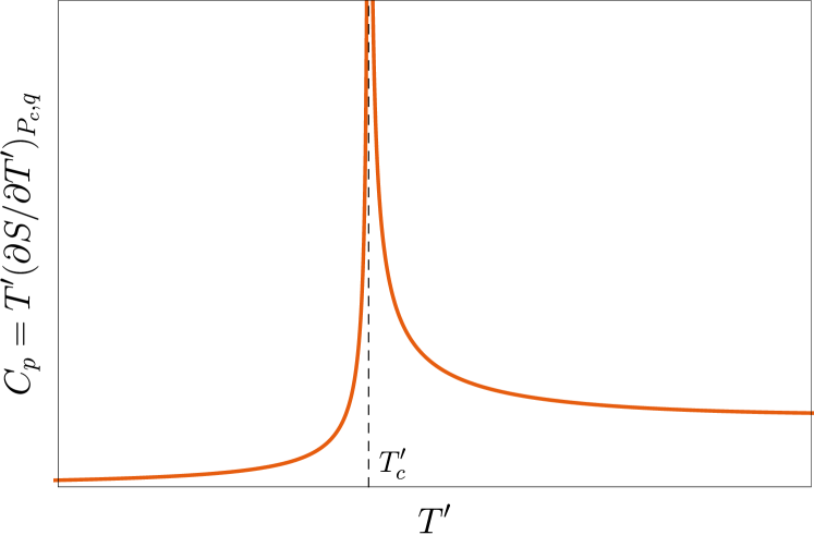
(e)

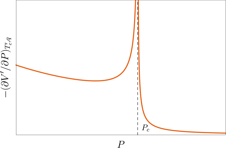
(f)

Figure 3: The thermodynamic behaviors near the critical points of regular black holes in Einstein’s gravity coupled with nonlinear electrodynamics.

3.2 Applications to specific regular black hole models

3.2.1 Bardeen black holes

A number of works have been devoted [21, 22, 40] to explore thermodynamic properties of Bardeen black holes. However, the main issue is the violation of the Bekenstein-Hawking area formula, where the formula, $S_{\rm BH}=\rm Area/4$, denotes that the entropy of black holes is proportional to the area of an event horizon in Einstein’s gravity. Let us give a brief review on how the issue arises. The reason is that the starting point is an incorrect first law,

$$dM=TdS+\varphi dq+VdP,$$ (3.12)

with which the corresponding thermodynamic quantities take [21, 22] the forms,

$$T = \frac{3r_{+}^{4}+l^{2}(r_{+}^{2}-2q^{2})}{4\pi r_{+}l^{2}\left(q^{2}+r_{+}^{2}\right)},$$ (3.13)

$$V = \frac{4}{3}\pi\left(q^{2}+r_{+}^{2}\right)^{3/2},$$ (3.14)

$$\varphi = \frac{3q(l^{2}+r_{+}^{2})\sqrt{q^{2}+r_{+}^{2}}}{2l^{2}r_{+}^{2}},$$ (3.15)

$$S = 2\pi\left(\frac{r_{+}}{2}-\frac{q^{2}}{r_{+}}\right)\sqrt{q^{2}+r_{+}^{2}}+\frac{3}{2}\pi q^{2}\log\left(\sqrt{q^{2}+r_{+}^{2}}+r_{+}\right).$$ (3.16)

It is clear that Eq. (3.14) deviates from the volume of a sphere, and in particular Eq. (3.16) does not obey the Bekenstein-Hawking area formula, which shows that the thermodynamic quantities, ($T,\varphi,P,S,q,V$), do not construct a correct and complete phase space. As is known, Einstein’s gravity coupled with nonlinear electrodynamics is still within the framework of general relativity, and thus the entropy of regular black holes should obey the Bekenstein-Hawking area formula. Let us recover the consistency in thermodynamics of regular black holes in Einstein’s gravity coupled with nonlinear electrodynamics.

We start with the improved first law given in Sec. 3.1, see Eqs. (3.1) and (3.2), and rewrite it in the following form,

$$dM=TdS+\Psi dq+VdP+K_{q}dq+K_{M}dM,$$ (3.17)

where $\Psi$, $K_{q}$ and $K_{M}$ take the forms,

$$\Psi = \frac{3M}{2q}\left[1-\frac{r_{+}^{5}}{\left(q^{2}+r_{+}^{2}\right){}^{5/2}}\right],$$

$$K_{q} = \frac{3M}{2q}\left[\frac{2q^{2}r_{+}^{3}+r_{+}^{5}}{\left(q^{2}+r_{+}^{2}\right){}^{5/2}}-1\right],$$

$$K_{M} = 1-\frac{r_{+}^{3}}{\left(q^{2}+r_{+}^{2}\right)^{3/2}},$$ (3.18)

for Bardeen black holes, i.e., $\mu=3$ and $\nu=2$ in Eqs. (2.29), (2.30), and (2.31). Now we can reproduce the Bekenstein–Hawking entropy in terms of the improved first law,

$$S=\int\frac{1-K_{M}}{T}=\pi r_{+}^{2},$$ (3.19)

and simultaneously eliminate the derivation of a sphere volume in Eq. (3.14),

$$V=(1-K_{M})\left(\frac{\partial M}{\partial P}\right)_{S,q}=\frac{4}{3}\pi r_{+}^{3}.$$ (3.20)

Next we give the correct and complete phase space and analyze thermodynamic behaviors for Bardeen black holes. We start directly with Eqs. (3.1) and (3.2), and compute $T^{\prime},V^{\prime}$, and $\Psi^{\prime}$ with Eq. (3.18),

$$T^{\prime} = \frac{T}{1-K_{M}}=\frac{\sqrt{r_{+}^{2}+q^{2}}\left(8\pi Pr_{+}^{4}+r_{+}^{2}-2q^{2}\right)}{4\pi r_{+}^{4}},$$

$$V^{\prime} = \frac{V}{1-K_{M}}=\frac{4}{3}\pi\left(r_{+}^{2}+q^{2}\right)^{3/2},$$

$$\Psi^{\prime} = \frac{\Psi+K_{q}}{1-K_{M}}=\frac{3Mq}{r_{+}^{2}+q^{2}},$$ (3.21)

and note that the phase space composed of ($T^{\prime}$, $\Psi^{\prime}$, $P$, $S$, $q$, $V^{\prime}$) depends on the nonlinear electrodynamic coupling and it is just the new extended phase space we expect. In the following we analyze thermodynamic behaviors for Bardeen black holes in terms of this phase space.

The equation of state should be expressed as the function of $T^{\prime}$ and $V^{\prime}$ instead of $T$ and $V$,

$$P=P(T^{\prime},V^{\prime}),$$ (3.22)

which indeed describes the behaviors of Bardeen black holes as we shall see. Substituting Eqs. (3.21) and (3.22) into the critical condition,

$$\left(\frac{\partial P}{\partial V^{\prime}}\right)_{T^{\prime}}=0,\qquad\left(\frac{\partial^{2}P}{\partial V^{\prime 2}}\right)_{T^{\prime}}=0,$$ (3.23)

we obtain the critical values of $T^{\prime},V^{\prime}$ and $P$,

$$T^{\prime}_{c} = \frac{5\sqrt{188\sqrt{10}-505}}{432\pi q},$$

$$V^{\prime}_{c} = \frac{4}{3}\left(2\sqrt{10}+5\right)^{3/2}\pi q^{3},$$

$$P_{c} = \frac{5\sqrt{10}-13}{432\pi q^{2}}.$$ (3.24)

We emphasize that this critical point coincides strictly with the inflection point at which the first-order phase transition vanishes. As shown in Fig. 4, $P(T^{\prime},V^{\prime})$ describes the whole process from a first-order phase transition to a second-order one of Bardeen black holes. If $T^{\prime}<T^{\prime}_{c}$, there exists a small-large phase transition that characterizes the oscillatory behavior of $(P,V^{\prime})$ in Fig. 4(a) and the swallow tail behavior of $(G^{\prime},P)$ in Fig. 4(b). If $T^{\prime}=T^{\prime}_{c}$, both the oscillatory behavior and the swallow tail behavior vanish. In particular, when $T^{\prime}$ and $P$ approach their critical values, $T^{\prime}=T^{\prime}_{c}$ and $P=P_{c}$, the small-large phase transition changes into a second-order one. Therefore, we can say that this critical point, $(T^{\prime}_{c},P_{c})$, is actually a true second-order phase transition point of Bardeen black holes.

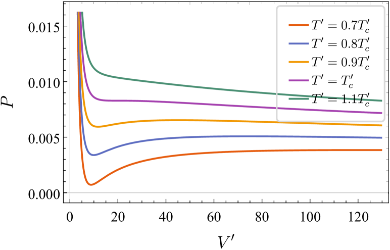
(a)

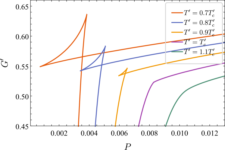
(b)

Figure 4: (a) The oscillatory behavior on the $P-V^{\prime}$ plane and (b) the swallow tail behavior on the $G^{\prime}-P$ plane of Bardeen black holes.

In addition, we calculate $P$ and $T^{\prime}$ of small and large phases of Bardeen black holes, and find that the results given by the new Gibbs free energy Eq. (3.3) are strictly equal to those given by the Maxwell equal area law Eq. (3.5). In Fig. 5(a), the black dots are computed by the new Gibbs free energy, and the solid curve is given by the Maxwell equal area law. Clearly, the two methods give the same coexistence curve.

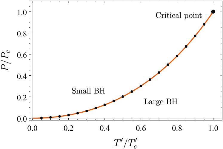
(a)

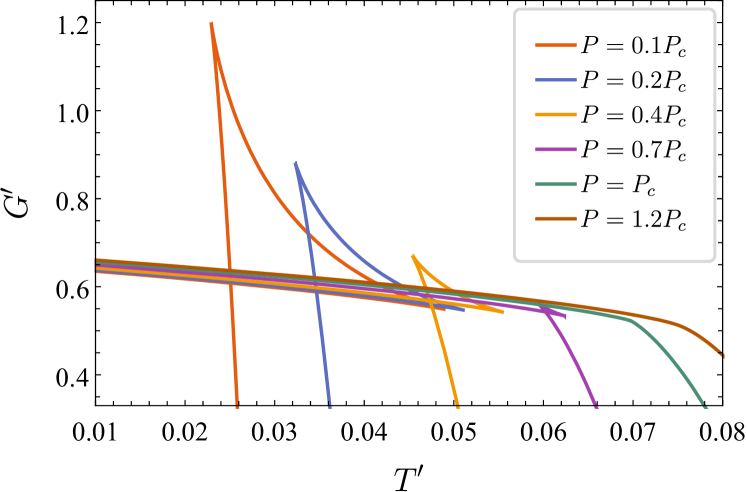
(b)

Figure 5: (a) The coexistence curve of small-large phase and (b) the swallow tail behavior on the $G^{\prime}-T^{\prime}$ plane of Bardeen black holes.

3.2.2 Hayward black holes

In Hayward black holes, the Maxwell equal area law was misinterpreted [20], which gave rise to the law’s violation and inconsistency with the Gibbs free energy. The reason is the same as in Bardeen black holes — an incorrect first law of thermodynamics was used.

Following the same procedure as in Sec. 3.2.1, we start with Eq. (3.17) and $\Psi,K_{q}$ and $K_{M}$,

$$\Psi = \frac{3Mq^{2}\left(2r_{+}^{3}+q^{3}\right)}{2\left(r_{+}^{3}+q^{3}\right)^{2}},$$

$$K_{q} = -\frac{36Mq^{5}}{\left(r_{+}^{3}+q^{3}\right)^{3}},$$

$$K_{M} = \frac{q^{3}}{r_{+}^{3}+q^{3}},$$ (3.25)

which correspond to Hayward black holes with $\mu=3$ and $\nu=3$ in Eqs. (2.29), (2.30), and (2.31), and then obtain the Bekenstein–Hawking entropy,

$$S=\int\frac{1-K_{M}}{T}=\pi r_{+}^{2},$$ (3.26)

and the volume without deviation from a sphere,

$$V=(1-K_{M})\left(\frac{\partial M}{\partial P}\right)_{S,q}=\frac{4\pi}{3}r_{+}^{3}.$$ (3.27)

Moreover, starting with Eqs. (3.1) and (3.2) together with

$$T^{\prime} = \frac{8\pi Pr_{+}^{5}+r_{+}^{3}-2q^{3}}{4\pi r_{+}^{4}},$$

$$V^{\prime} = \frac{4}{3}\pi\left(r_{+}^{3}+q^{3}\right),$$

$$\Psi^{\prime} = \frac{1}{2}q^{2}\left(8\pi P+\frac{3}{r_{+}^{2}}\right),$$ (3.28)

which can be calculated with the help of Eq. (3.25), we provide the new extended phase space, ($T^{\prime}$, $\Psi^{\prime}$, $P$, $S$, $q$, $V^{\prime}$), which is similar to that in Bardeen black holes. Therefore, the equation of state of Hayward black holes should be expressed as

$$P=P(T^{\prime},V^{\prime}),$$ (3.29)

and the critical values can be obtained from Eq. (3.23),

$$T^{\prime}_{c} = \frac{3}{8\sqrt[3]{20}\pi q},$$

$$V^{\prime}_{c} = 28\pi q^{3},$$

$$P_{c} = \frac{3}{80\sqrt[3]{50}\pi q^{2}}.$$ (3.30)

The critical point coincides with the point at which the first-order phase transition vanishes. The oscillatory behavior on the $P-V^{\prime}$ planes is shown in Fig. 6(a). Using our newly defined Gibbs free energy Eq. (3.3), we plot the swallow tail in Fig. 6(b). When $T^{\prime}<T^{\prime}_{c}$, there exists the small-large phase transition which is characterized by the oscillatory behavior in Fig. 6(a) and by the swallow tail in Fig. 6(b). When $T^{\prime}=T^{\prime}_{c}$ and $P=P_{c}$, the first-order phase transition changes into a second-order one.

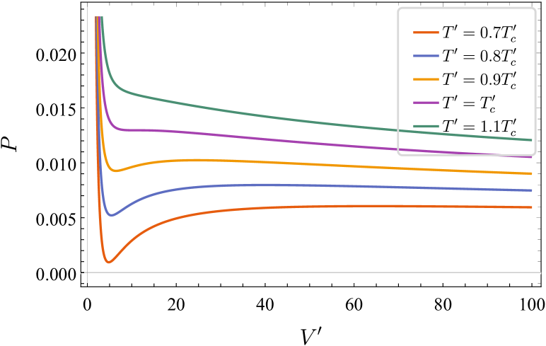
(a)

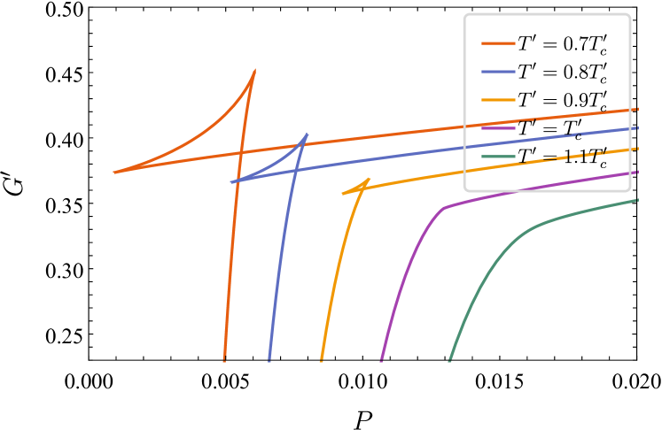
(b)

Figure 6: (a) The oscillatory behavior on the $P-V^{\prime}$ plane and (b) the swallow tail behavior on the $G^{\prime}-P$ plane of Hayward black holes.

In addition, in Fig. 7(a) the black dots are given by the new Gibbs free energy Eq. (3.3), and the solid curve is given by the Maxwell equal area law. The results computed by the two methods strictly coincide with each other. The coexistence curve terminates at the critical point $(T^{\prime}_{c},P_{c})$, where the area of a swallow tail equals zero as shown in Fig. 6(b) and Fig. 7(b). As this critical point corresponds to the point at which the first-order phase transition vanishes, we conclude that the Maxwell equal area law holds strictly for Hayward black holes.

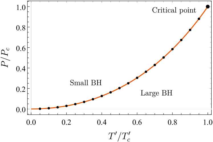
(a)

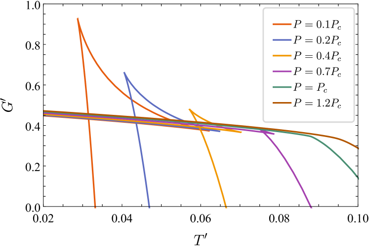
(b)

Figure 7: (a) The coexistence curve of small-large phase and (b) the swallow tail behavior on the $G^{\prime}-T^{\prime}$ plane of Hayward black holes.

3.3 A universal number at critical points

3.3.1 Bardeen black holes

Comparing Bardeen black holes with van der Waals fluid and defining the specific volume [24], $v\equiv 2\sqrt{r^{2}+q^{2}}$, we write the equation of state as follows:

$$P=\frac{T^{\prime}}{v}-\frac{v^{2}-12q^{2}}{2\pi\left(v^{2}-4q^{2}\right)^{2}}.$$ (3.31)

Then using the critical condition,

$$\left(\frac{\partial P}{\partial v}\right)_{T^{\prime}}=0,\qquad\left(\frac{\partial^{2}P}{\partial v^{2}}\right)_{T^{\prime}}=0,$$ (3.32)

we calculate the critical values,

$$T^{\prime}_{c}=\frac{5\sqrt{188\sqrt{10}-505}}{432\pi q},\qquad v_{c}=2\sqrt{5+2\sqrt{10}}q,\qquad P_{c}=\frac{5\sqrt{10}-13}{432\pi q^{2}}.$$ (3.33)

As a result, we obtain a number at this critical point,

$$\frac{P_{c}v_{c}}{T^{\prime}_{c}}=\frac{2}{5},$$ (3.34)

which is clearly independent of $q$ — the nonlinear electrodynamic coupling.

3.3.2 Hayward black holes

Similarly, comparing Hayward black holes with van der Waals fluid and defining the specific volume, $v\equiv 2r$, we write the equation of state as follows:

$$P=\frac{T^{\prime}}{v}-\frac{1}{2\pi v^{2}}+\frac{8q^{3}}{\pi v^{5}}.$$ (3.35)

The critical condition Eq. (3.32) determines the critical values,

$$T^{\prime}_{c}=\frac{3}{8\sqrt[3]{20}\pi q},\qquad v_{c}=2\sqrt[3]{20}q,\qquad P_{c}=\frac{3}{80\sqrt[3]{50}\pi q^{2}}.$$ (3.36)

Although these values are different from those in Eq. (3.33), they still give rise to the same number as in Eq. (3.34).

3.3.3 Hypothesis

According to the above analysis on the combination ${P_{c}v_{c}}/{T^{\prime}_{c}}$ of the three critical values, $T^{\prime}_{c},v_{c}$, and $P_{c}$, for both Bardeen and Hayward black holes, we may conclude that Eq. (3.34) gives a universal number for any regular black hole in Einstein’s gravity coupled with nonlinear electrodynamics.

4 Summary

We revisit thermodynamics of regular black holes in Einstein’s gravity coupled with nonlinear electrodynamics, and establish an improved first law of thermodynamics by introducing a new extended phase space. In terms of this improved first law and new extended phase space, we recover the consistency of the Bekenstein-Hawking area formula and Maxwell equal area law for a general model in Einstein’s gravity coupled with nonlinear electrodynamics. Then we apply the improved first law together with the new extended phase space to Bardeen and Hayward black holes, and find that the inconsistency and deviation of thermodynamic quantities, such as volume, are eliminated. In particular, based on the comparison between Bardeen (Hayward) black holes with van der Waals fluid we deduce a general number at critical points of phase transitions for any regular black hole in Einstein’s gravity coupled with nonlinear electrodynamics. Our results meet the fact that Einstein’s gravity coupled with nonlinear electrodynamics is still within the framework of general relativity, and thus the Bekenstein-Hawking area formula and Maxwell equal area law should be valid as they are in Einstein’s gravity. Our work makes clear various misinterpretations that appeared in earlier literature on thermodynamics of regular black holes in Einstein’s gravity coupled with nonlinear electrodynamics.

Acknowledgments

This work was supported in part by the National Natural Science Foundation of China under Grant No. 12175108.

References

- [1] E. Ayon-Beato and A. Garcia, Regular black hole in general relativity coupled to nonlinear electrodynamics, Phys. Rev. Lett. 80 (1998) 5056 [gr-qc/9911046].
- [2] E. Ayon-Beato and A. Garcia, New regular black hole solution from nonlinear electrodynamics, Phys. Lett. B 464 (1999) 25 [hep-th/9911174].
- [3] K.A. Bronnikov, Regular magnetic black holes and monopoles from nonlinear electrodynamics, Phys. Rev. D 63 (2001) 044005 [gr-qc/0006014].
- [4] M. Okyay and A. Övgün, Nonlinear electrodynamics effects on the black hole shadow, deflection angle, quasinormal modes and greybody factors, JCAP 01 (2022) 009 [2108.07766].
- [5] S.W. Hawking and G.F.R. Ellis, The large scale structure of space-time, vol. 1, Cambridge university press (1973).
- [6] E. Ayon-Beato and A. Garcia, The Bardeen model as a nonlinear magnetic monopole, Phys. Lett. B 493 (2000) 149 [gr-qc/0009077].
- [7] A. Burinskii and S.R. Hildebrandt, New type of regular black holes and particle - like solutions from NED, Phys. Rev. D 65 (2002) 104017 [hep-th/0202066].
- [8] E. Ayon-Beato and A. Garcia, Four parametric regular black hole solution, Gen. Rel. Grav. 37 (2005) 635 [hep-th/0403229].
- [9] M. Hassaine and C. Martinez, Higher-dimensional charged black holes solutions with a nonlinear electrodynamics source, Class. Quant. Grav. 25 (2008) 195023 [0803.2946].
- [10] L. Balart and E.C. Vagenas, Regular black holes with a nonlinear electrodynamics source, Phys. Rev. D 90 (2014) 124045 [1408.0306].
- [11] Z.-Y. Fan and X. Wang, Construction of Regular Black Holes in General Relativity, Phys. Rev. D 94 (2016) 124027 [1610.02636].
- [12] R.-G. Cai, D.-W. Pang and A. Wang, Born-Infeld black holes in (A)dS spaces, Phys. Rev. D 70 (2004) 124034 [hep-th/0410158].
- [13] Y.S. Myung, Y.-W. Kim and Y.-J. Park, Thermodynamics and phase transitions in the Born-Infeld-anti-de Sitter black holes, Phys. Rev. D 78 (2008) 084002 [0805.0187].
- [14] H.A. Gonzalez, M. Hassaine and C. Martinez, Thermodynamics of charged black holes with a nonlinear electrodynamics source, Phys. Rev. D 80 (2009) 104008 [0909.1365].
- [15] P. Wang, H. Wu and H. Yang, Thermodynamics and Phase Transitions of Nonlinear Electrodynamics Black Holes in an Extended Phase Space, JCAP 04 (2019) 052 [1808.04506].
- [16] P. Wang, H. Wu and H. Yang, Thermodynamics and Phase Transition of a Nonlinear Electrodynamics Black Hole in a Cavity, JHEP 07 (2019) 002 [1901.06216].
- [17] A. Bokulić, T. Jurić and I. Smolić, Black hole thermodynamics in the presence of nonlinear electromagnetic fields, Phys. Rev. D 103 (2021) 124059 [2102.06213].
- [18] S.H. Hendi and M.H. Vahidinia, Extended phase space thermodynamics and P-V criticality of black holes with a nonlinear source, Phys. Rev. D 88 (2013) 084045 [1212.6128].
- [19] D.-C. Zou, S.-J. Zhang and B. Wang, Critical behavior of Born-Infeld AdS black holes in the extended phase space thermodynamics, Phys. Rev. D 89 (2014) 044002 [1311.7299].
- [20] Z.-Y. Fan, Critical phenomena of regular black holes in anti-de Sitter space-time, Eur. Phys. J. C 77 (2017) 266 [1609.04489].
- [21] A.G. Tzikas, Bardeen black hole chemistry, Phys. Lett. B 788 (2019) 219 [1811.01104].
- [22] C.L.A. Rizwan, A. Naveena Kumara, K. Hegde and D. Vaid, Coexistent Physics and Microstructure of the Regular Bardeen Black Hole in Anti-de Sitter Spacetime, Annals Phys. 422 (2020) 168320 [2008.06472].
- [23] A. Naveena Kumara, C.L.A. Rizwan, K. Hegde and K.M. Ajith, Repulsive Interactions in the Microstructure of Regular Hayward Black Hole in Anti-de Sitter Spacetime, Phys. Lett. B 807 (2020) 135556 [2003.10175].
- [24] D. Kubiznak and R.B. Mann, P-V criticality of charged AdS black holes, JHEP 07 (2012) 033 [1205.0559].
- [25] N. Altamirano, D. Kubiznak and R.B. Mann, Reentrant phase transitions in rotating anti–de Sitter black holes, Phys. Rev. D 88 (2013) 101502 [1306.5756].
- [26] D. Kubiznak, R.B. Mann and M. Teo, Black hole chemistry: thermodynamics with Lambda, Class. Quant. Grav. 34 (2017) 063001 [1608.06147].
- [27] D.A. Rasheed, Nonlinear electrodynamics: Zeroth and first laws of black hole mechanics, hep-th/9702087.
- [28] Y. Zhang and S. Gao, First law and Smarr formula of black hole mechanics in nonlinear gauge theories, Class. Quant. Grav. 35 (2018) 145007 [1610.01237].
- [29] B. Toshmatov, Z. Stuchlík and B. Ahmedov, Comment on “Construction of regular black holes in general relativity”, Phys. Rev. D 98 (2018) 028501 [1807.09502].
- [30] K.A. Bronnikov, Comment on “Construction of regular black holes in general relativity”, Phys. Rev. D 96 (2017) 128501 [1712.04342].
- [31] S.A. Hayward, Formation and evaporation of regular black holes, Phys. Rev. Lett. 96 (2006) 031103 [gr-qc/0506126].
- [32] N. Altamirano, D. Kubizňák, R.B. Mann and Z. Sherkatghanad, Kerr-AdS analogue of triple point and solid/liquid/gas phase transition, Class. Quant. Grav. 31 (2014) 042001 [1308.2672].
- [33] Y.-G. Miao and Z.-M. Xu, On thermal molecular potential among micromolecules in charged AdS black holes, Phys. Rev. D 98 (2018) 044001 [1712.00545].
- [34] S.-W. Wei and Y.-X. Liu, Insight into the Microscopic Structure of an AdS Black Hole from a Thermodynamical Phase Transition, Phys. Rev. Lett. 115 (2015) 111302 [1502.00386].
- [35] J.-L. Zhang, R.-G. Cai and H. Yu, Phase transition and thermodynamical geometry of Reissner-Nordström-AdS black holes in extended phase space, Phys. Rev. D 91 (2015) 044028 [1502.01428].
- [36] M. Eune, W. Kim and S.-H. Yi, Hawking-Page phase transition in BTZ black hole revisited, JHEP 03 (2013) 020 [1301.0395].
- [37] R. Li and J. Wang, Thermodynamics and kinetics of Hawking-Page phase transition, Phys. Rev. D 102 (2020) 024085.
- [38] R. Li and J. wang, Generalized free energy landscape of a black hole phase transition, Phys. Rev. D 106 (2022) 106015 [2206.02623].
- [39] S.-J. Yang, R. Zhou, S.-W. Wei and Y.-X. Liu, Kinetics of a phase transition for a Kerr-AdS black hole on the free-energy landscape, Phys. Rev. D 105 (2022) 084030 [2105.00491].
- [40] J. Pu, S. Guo, Q.-Q. Jiang and X.-T. Zu, Joule-Thomson expansion of the regular(Bardeen)-AdS black hole, Chin. Phys. C 44 (2020) 035102 [1905.02318].