Numerical investigation of mixed-phase turbulence induced by a plunging jet

Abstract

In nature and engineering applications, plunging jet acts as a key process causing interface breaking and generating mixed-phase turbulence. In this paper, high-resolution numerical simulation of water jet plunging into a quiescent pool was perform to investigate the statistical property of the mixed-phase turbulence, with special focus on the closure problem of the Reynolds-averaged equation. We conducted phase-resolved simulations, with the air–water interface captured using a coupled level-set and volume-of-fluid method. Nine cases were performed to analyse the effects of the Froude number and Reynolds number. The simulation results showed that the turbulent statistics are insensitive to the Reynolds number under investigation, while the Froude number influences the flow properties significantly. To investigate the closure problem of the mean momentum equation, the turbulent kinetic energy (TKE) and turbulent mass flux (TMF) and their transport equations were further investigated. It was discovered that the balance relationship of the TKE budget terms remained similar to many single-phase turbulent flows. The TMF is an additional unclosed term in the mixed-phase turbulence. Our simulation results showed that the production term of its transport equation was highly correlated to the TKE. Based on this finding, a closure model of its production term was further proposed.

1 Introduction

Mixed-phase turbulence is a common phenomenon in nature and engineering applications. Difference from two-phase turbulent flow without surface breaking  (Brocchini and Peregrine, 2001), mixed-phase turbulence is accompanied by violent surface deformation and surface breakup, leading to complex mass and momentum transfer across interface.

Water jet plunging is a typical process that induces mixed-phase turbulence  (Kiger and Duncan, 2012, Delacroix et al., 2016). For some advanced ships, plunging jet adds another source of air entrainment in the transom region and beyond (Hsiao et al., 2013). Plunging liquid jets were early investigated in chemical engineering applications, such as waste water treatment (van der Lans et al., 1979), mixing and reacting of liquids and gases (McKeogh and Ervine, 1981). The research in this area has focused on the mechanism of air entrainment and the characteristics of the resulting bubble flows. It was found that the impact velocity of the liquid jet plays a dominant role in the air entrainment inception conditions. It was reported that the entrainment velocity is a key criterion of air entrainment (Lorenceau et al., 2004). When the critical condition was reached, a minimum amount of energy was available in the flow to do work against surface tension and/or the potential energy of gravity to entrap air. Laboratory experiments were conducted to analyse the critical entrainment velocity for both high-viscosity liquids  (Biń, 1993, Joseph et al., 1991, Jeong and Moffatt, 1992, Eggers, 2001, Lorenceau et al., 2003, 2004) and low-viscosity liquids (Biń, 1993, Sene, 1988, Lin and Reitz, 1998, El Hammoumi et al., 2002, Chirichella et al., 2002a).  Clanet and Lasheras (1997) proposed a model to predict the penetration depth of the air bubbles entrained by a water jet impacting into a flat water pool. This model showed that the depth is determined by the initial jet momentum and the bubble terminal velocity as a function of its size. Comprehensive reviews of the related research can be found in Biń (1993) and Kiger and Duncan (2012).

The aforementioned studies focused on the vertical plunging jet, and recently, the horizontal and shallow-angle plunging jets have also been investigated. Deshpande et al. (2012) studied a shallow-angle plunging jet and revealed a periodic pattern of air entrainment, which does not happen when the impinging angle is steep. After that, Deshpande and Trujillo (2013) corroborated that the periodicity scaled linearly with the Froude number through numerical simulations. They also studied both computationally and analytically the underlying causes responsible for large cavity formation at shallow angles. They found a strong stagnation pressure region for the shallow impacts, which serves to deflect the entire incoming jet flow radially outwards, producing a large cavity and subsequently creating splashing events.  Hsiao et al. (2013) studied a stationary and moving horizontal jet plunging into a quiescent water pool. Their numerical and experimental results showed that the frequency of air entrainment depended on the jet diameter and relative velocity with respect to the free surface.

In addition to the plunging jet, mixed-phase turbulence with air entrainment also occurs in hydraulic jump, wave breaking, near-surface shear flow and wake behind a column. Chachereau and Chanson (2011) conducted experimental studies on air entrainment in hydraulic jumps and observed that air entrainment takes place as the Froude number exceeds a critical value. They also found that the volume of air entrainment increases with an increasing Froude number. Garrett et al. (2000), Deane and Stokes (2002), Wang et al. (2016b) and Deike et al. (2016b) studied the bubbles induced by breaking waves and observed that the bubble size spectrum is proportional to $r^{-10/3}$, where $r$ is the effective radius of the bubbles. Garrett et al. (2000) proposed a cascade scenario to understand the power law. Yu et al. (2019) performed DNS of a canonical three-dimensional two-phase viscous turbulent flow with the turbulent kinetic energy (TKE) supplied by an underlying near-surface shear flow. They investigated the dependence of air entrainment and bubble size on the Froude number and Weber number. They proposed a heuristic model that qualitatively matched and explained the salient evolution behaviour of the bubble size spectrum. Hendrickson et al. (2019) performed implicit large eddy simulations (iLES) with a conservative volume-of-fluid interface-capturing method to investigate the mixed-phase turbulent wake behind a dry transom stern of a surface ship. They conducted detailed analyse on the air entrainment including entrainment rate and bubble size spectrum.

From the above reviews, it is understood that the mechanism and physical process of air entrainment and bubble generation have been studied extensively in the mixed-phase turbulence. However, the studies on the statistical characteristics and transport mechanics of the turbulence were limited in the literature. As the most common phenomenon that induces two-phase turbulence in nature, breaking waves modulate the transfer of mass, momentum, and energy between the ocean and atmosphere. Deike (2022) summarized the recent researches on breaking waves. Based on canonical experiments (Rapp and Melville, 1990, Melville, 1994, Melville et al., 2002, Banner and Peirson, 2007, Drazen et al., 2008, Tian et al., 2010), simulations with direct numerical simulations (DNS) (Chen et al., 1999, Iafrati, 2009, Deike et al., 2015, 2016a, Wang et al., 2016a, Yang et al., 2018, Chan et al., 2021, Mostert et al., 2022) and large eddy simulations (LES) (Lubin and Glockner, 2015, Derakhti and Kirby, 2016), the dynamics of wave breaking were investigated. However, as a statistically unsteady process, it is difficult to analyse the statistical properties of turbulence induced by breaking wave. To date, the research of turbulent statistics corresponding to breaking wave is limited to its impact on the wind turbulence (Yang et al., 2018), and the study on the mixed-phase region is limited. In terms of statistically stationary mixed-phase turbulence, Deshpande et al. (2012) investigated the mean velocity, mean volume of fluid and the TKE for a plunging jet. Yu et al. (2019) investigated the characteristics of free-surface turbulence and elucidated the qualitatively distinct characteristics of strong versus weak free-surface turbulence. Strong anisotropy was found in weak free-surface flow while mixed-phase turbulence became almost isotropic in strong free-surface turbulence. When it comes to statistical averaging of variable density fluid motion equations, an additional unclosed term appears, that is, the turbulent mass flux (TMF) $\overline{\rho u_{i}^{\prime}}$ (Taulbee and Vanosdol, 1991). Modelling of TMF was earlier investigated in compressible flow (Jones, 1979, Grasso and Speziale, 1989, Nichols, 1990). Comprehensive reviews can be found in Chassaing (2001). Recently, Hendrickson and Yue (2019) studied the incompressible highly variable density turbulence in the wake behind a three-dimensional dry transom stern. They developed an explicit algebraic closure model for the TMF.

The objective of present study is to investigate the statistical characteristics of the mixed-phase turbulence with air entrainment caused by a plunging jet. Specifically, we aim to study in detail the basic statistics reflecting turbulent characteristics, such as TKE, TMF and their transport equations. The Froude number effect is examined through different cases. The closure problem of TMF is also discussed. The remainder of this paper is organized as follows. In section 2, the numerical method and physical setup of present simulation of the plunging jet are described. Then, the results are presented and discussed in section 3, followed by the conclusions in section 4.

2 Details of numerical simulations

2.1 Numerical method

We perform high-resolution large eddy simulation (LES) by solving the three-dimensional two-phase incompressible Navier–Stokes equations to study a water jet plunging into a quiescent pool. The coupled level-set (LS) and volume of fluid (VOF) method is used to capture the air–water interface on a Cartesian grid. The three-dimensional incompressible Navier–Stokes equations with varying density and viscosity are expressed as:

$$\nabla\cdot\mathbf{u}=0,$$ (1)

$$\frac{\partial(\rho\mathbf{u})}{\partial t}+\nabla\cdot(\rho\mathbf{u}\mathbf{u})=-\nabla p+\nabla\cdot(2\mu\mathbf{S})+\rho\mathbf{g}+\mathbf{f}_{s},$$ (2)

where $\rho$ and $\mu$ are density and dynamic viscosity, respectively, $\mathbf{u}=[u,v,w]$ is the velocity, $p$ is the pressure, $\mathbf{S}=(\nabla\mathbf{u}+\nabla\mathbf{u}^{T})/2$ is the strain-rate tensor, $\mathbf{g}=[0,-g,0]$ is the gravitational acceleration. The last term in equation (2) is the surface tension force, define as

$$\mathbf{f}_{s}=\sigma\kappa\nabla H(\phi),$$ (3)

where $\sigma$ is the surface tension, $\kappa=\nabla\cdot(\nabla\phi)$ at $\phi=0$ is the interface curvature with $\phi$ being the LS function, and $H(\phi)$ is the Heaviside function, defined as

$$H\left(\phi,\Delta_{s}\right)=\begin{cases}0,&\phi\leq 0,\\ 1,&\phi>0.\end{cases}$$ (4)

In LES, the dynamic viscosity is expressed as

$$\mu=\rho(\nu+\nu_{t}),$$ (5)

where $\nu$ is the kinematic viscosity and $\nu_{t}$ the eddy viscosity. In present work, an eddy-viscosity subgrid-scale model for turbulent shear flow developed by Vreman (2004) is used to determine $\nu_{t}$. We note here that in low Reynolds number cases, it shows $\nu_{t}\ll\nu$, and as a result, $\nu_{t}$ is omitted in these cases following Hendrickson et al. (2019). Therefore, the case with low Reynolds numbers in the present work can be also regarded as high-resolution iLES.

The interface between the two fluid phases is captured using the CLSVOF method. The following convection equations of the LS function $\phi$ and VOF function $\psi$ are solved:

$$\frac{\partial\phi}{\partial t}+\nabla\cdot(\phi\mathbf{u})=0,$$ (6)

$$\frac{\partial\psi}{\partial t}+\nabla\cdot(\psi\mathbf{u})=0.$$ (7)

The LS function $\phi$ is defined as the signed distance from either fluid phase to the interface; its sign is negative and positive for air and water, respectively. The VOF function $\psi$ is defined as the volume fraction of water in a grid cell ranging from 0 to 1. Let subscripts $a$ and $w$ denote air and water, respectively. The density and viscosity are determined using the LS function as follows:

$$\rho=\rho_{a}+\left(\rho_{w}-\rho_{a}\right)H(\phi),$$ (8)

$$\mu=\mu_{a}+\left(\mu_{w}-\mu_{a}\right)H(\phi).$$ (9)

As noted in the literature (Rudman, 1998, Arrufat et al., 2018, Nangia et al., 2019, Yang et al., 2021), if the density is determined solely using equation (8), the simulation is unstable for two-fluid flows with a high density contrast. An effective approach for improving the numerical stability is to calculate the mass and momentum fluxes using a consistent scheme and evolve the density by solving the following convection equation:

$$\frac{\partial\rho}{\partial t}+\nabla\cdot(\rho\mathbf{u})=0.$$ (10)

In the present study, equation (8) is used to determine the density at the beginning of each time step, while equation (10) is evolved together with the momentum equation to provide the density within a time step. As such, the interface is accurately captured, and meanwhile, the simulation is stable. More details about the numerical method can be found in  Yang et al. (2021).

2.2 Physical setup

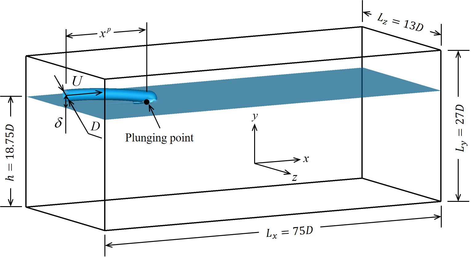
Figure 1: Definition sketch of computational model.

Figure 1 schematically shows the computational domain and definition of key parameters. As shown, a water jet spurts out horizontally and plunges into a quiescent water pool. Except for the water column and pool, other space of the computational domain is initially filled with air, some of which tends to be entrained into the water with the jet and then evolves into air cavities and bubbles beneath the free surface. We use the jet diameter $D$ as the characteristic length scale and the horizontal outlet velocity of jet $U$ as the characteristic velocity scale. Hereafter, all variables are non-dimensionalized using $U$ and $D$ unless otherwise stated. The computational domain size is $L_{x}\times L_{y}\times L_{z}=75.0\times 27.0\times 13.0$, where $x$, $y$, $z$ represent streamwise, vertical and spanwise directions of the domain, respectively. The water depth is $h=18.75$. The distance between the centre of jet orifice and the free surface is $\delta=1.0$. The boundary condition is no-penetration at the top, bottom, front and back of the domain, while an constant inlet velocity is applied in the jet orifice area of the left boundary and a zero gradient condition is specified at the right outlet boundary. The whole computational domain is discretized using a uniform Cartesian grid and the grid resolution in three directions is $\Delta x=\Delta y=\Delta z=0.1$. In the present study, to consider the effect of the Reynolds number $\text{Re}={UD}/{\nu}$ and the Froude number $\text{Fr}=\sqrt{{u^{2}}/{gD}}$, we conduct 9 cases. Key parameters are listed in table 1. Cases 1, 2, 6 are performed to examine the effect of Reynolds number and cases 3-9 are conducted to investigate the Froude number effect. The Reynolds number and Froude number for case 1 remain the same as the case considered in Deshpande et al. (2012) to facilitate validation.

Table 1: Parameters in the simulations of plunging jet.

case		Re		Fr		We
1		$1.6\times 10^{5}$		6.4		$8.89\times 10^{3}$
2		$1.6\times 10^{4}$		6.4		$8.89\times 10^{3}$
3		$1.6\times 10^{3}$		3.2		$8.89\times 10^{3}$
4		$1.6\times 10^{3}$		4.2		$8.89\times 10^{3}$
5		$1.6\times 10^{3}$		5.3		$8.89\times 10^{3}$
6		$1.6\times 10^{3}$		6.4		$8.89\times 10^{3}$
7		$1.6\times 10^{3}$		7.5		$8.89\times 10^{3}$
8		$1.6\times 10^{3}$		8.6		$8.89\times 10^{3}$
9		$1.6\times 10^{3}$		9.6		$8.89\times 10^{3}$

3 Results and discussion

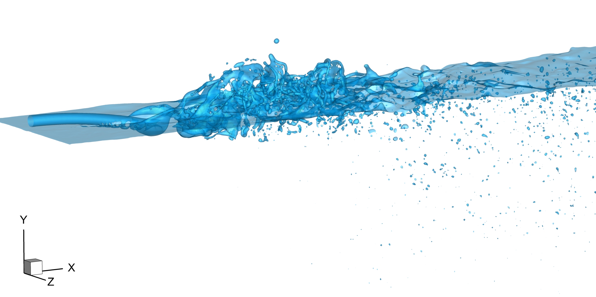
Figure 2: Instantaneous air–water interface at a certain time under the statistical steady state (iso-surface with $\phi=0$ in case 6).

3.1 Formation of mixed-phase region

An instantaneous flow field under the statistically steady state is shown in figure 2, in which the interface between air and water is visualized using the iso-surface of $\phi=0$. This figure illustrates entrained air pockets and bubbles under the surface, as well as water splash and droplets above the surface. It can be seen that a large air pocket is entrained into the water near the plunging point, and it breaks up into small air pockets and bubbles in the downstream. Above the free surface, water splash and droplets hit the downstream surface causing secondary plunging. The plunging event results in violent breaking of the free surface and highly mixed air–water turbulent flow. To better understand the highly mixed air–water turbulence in the near-surface region, we follow Hendrickson and Yue (2019) to define a mixed-phase region as the variable density region, where the mean volume of fluid $\overline{\psi}$ satisfies $0.05\leq\overline{\psi}\leq 0.95$. Here, the overline defines time averaging, which is performed over a time duration of $T=1200.0$, after the turbulence is fully developed. The sampling rate is $\Delta T=1.0$, which provides 1200 samples for time averaging. Figure 3 shows the mixed-phase region and mean free surface in case 6. It can be seen that as the streamwise coordinate $x$ increases, the size of the mixed-phase region increases and reaches a peak shortly after the jet plunging point and then decreases downstream. The mean free surface with $\overline{\psi}=0.5$ is also shown in figure 3(a) using the dash-dotted line. There exists a hollow of the mean free surface near the jet plunging point and a hump shortly downstream. They correspond to air entrainment and water splash-up, respectively.

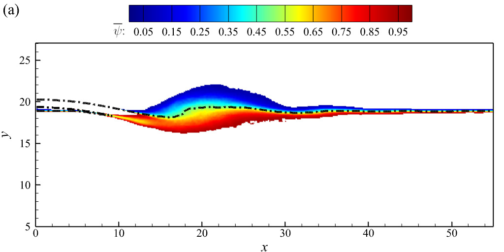
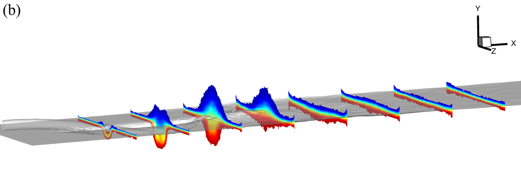
Figure 3: Mixed-phase region in case 6: (a) Contour of mean volume of fluid $0.05<\overline{\psi}<0.95$ at the mid span. (b) Transverse cuts of mixed-phase region in different streamwise position. Dash-dotted line in (a) and iso-surface in (b) represent the mean free surface with $\overline{\psi}=0.5$.

3.2 The Reynolds number effect

The Reynolds number is an important parameter in turbulent flow. However, in many previous studies of mixed-phase turbulence (Brocchini and Peregrine, 2001, Deike et al., 2015, Yu et al., 2019), it is found that the Reynolds number effect is less significant than the Froude number effect. To minimize the effect of LES modelling, it is a common treatment to reduce the Reynolds number. In this study, we test three Reynolds numbers to find its effects on turbulent statistics. Meanwhile, we compare these results with previous experimental and numerical studies to validate our simulations.

Figure 4 shows the vertical profiles of the mean volume of fluid $\overline{\psi}$ and mean streamwise velocity $\overline{u}$ at the mid span and different streamwise locations for the three Reynolds numbers. As shown in figure 4(a), the mean volume of fluid $\overline{\psi}$ varies mainly inside the mixed-phase region. The results of $\overline{\psi}$ for different Reynolds numbers are close with each other. They also agree with the numerical results of Deshpande et al. (2012). Figure 4(b) shows that the results of the mean velocity for different Reynolds numbers are also close with each other, which indicates that variation in the Reynolds number (from $1.6\times 10^{3}$ to $1.6\times 10^{5}$) does not impose significant effects on the mean flow. The results also agree with the experimental and numerical results of Deshpande et al. (2012).

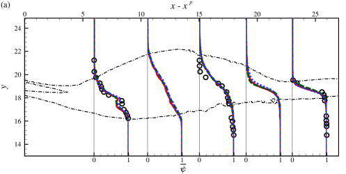
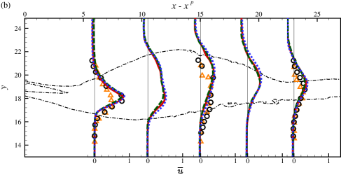
Figure 4: Vertical profiles of (a) mean volume of fluid and (b) mean streamwise velocity at the mid span and different streamwise locations for different Reynolds numbers. Solid: $\text{Re}=1.6\times 10^{5}$, dashed: $\text{Re}=1.6\times 10^{4}$, dotted: $\text{Re}=1.6\times 10^{3}$, circles and triangles represent numerical and experimental data, respectively, of same case with $\text{Re}=1.6\times 10^{5}$ in  Deshpande et al. (2012). Dash-dotted lines represent the edge of the mixed-phase region in case 6.

We also calculate the time-averaged bubble-size density spectra $\overline{N}(r_{eff})$, which is defined as

$$\overline{N}\left(r_{eff}\right)=\frac{1}{T}\int_{t}^{t+T}\frac{n\left(r_{eff},t;b\right)}{V\cdot b}\mathrm{~{}d}t,$$ (11)

where $n\left(r_{eff},t;b\right)$ is the number of bubbles, whose effective radii fall between $r_{eff}$ and $r_{eff}+b$ in a given fluid volume $V$ at time $t$. In the present work, $b=0.001$ is chosen. The fluid volume $V$ for bubble statistics is a cuboid in the computational domain of $x\in[15,45],y\in[0,h],z\in[0,L_{z}]$, which contains most of the air cavities and bubbles beneath the interface. The effective spherical radius is defined as

$$r_{eff}=\left[(3/4\pi)v_{e}\right]^{1/3},$$ (12)

where $v_{e}$ is the volume of an individual bubble. To determine the number and volume of each bubble, a connected component algorithm (Samet and Tamminen, 1988) is used to identify and label the entrained air cavities. Figure 5 shows the results of the bubble-size density spectra $\overline{N}(r_{eff})$ for different Reynolds numbers. It can be seen that the results for different Reynolds numbers are close to each other, indicating that the Reynolds number effect on the bubble-size density spectra is negligible. The solid line in figure 5 represents the $r^{-10/3}$ power law, which is satisfied in cases at different Reynolds numbers.

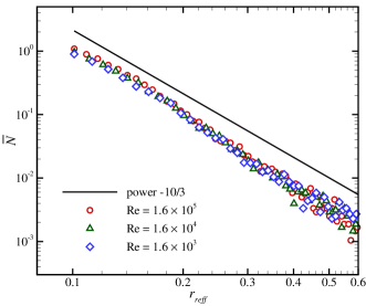
Figure 5: Average bubble-size density spectra as a function of effective radius in cases of different Reynolds number. ($\text{Fr}=6.4$)

The results of the mean velocity, volume of fluid, and the bubble-size density spectra for different Reynolds numbers (ranging from $1.6\times 10^{3}$ to $1.6\times 10^{5}$) indicate that the Reynolds number imposes limited impact on turbulence statistics. We have also examined the Reynolds number effects on other turbulent statistics, including TKE and TMF. It is found that the impact of the Reynolds number is less significant than the Froude number. Therefore, in the following context, we focus on the effect of the Froude number.

3.3 Scaling of cross-sectional area of mixed-phase region with Froude number

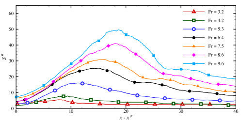
Figure 6: Profiles of the mixed-phase region area along the streamwise direction in cases of different Froude number.

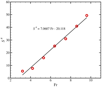
Figure 7: Peak variables of the mixed-phase region area varying with Froude number and the fit curve.

We start analysing the Froude number effect from the size of the mixed-phase region. Figure 6 shows the the streamwise variation of the cross-sectional area $S^{R}(x)$ of the mixed-phase region. The jet plunging point $x^{p}$ is influenced by the Froude number, and we use $x-x^{p}$ as the independent variable to facilitate comparisons among different cases. As shown in figure 6, as the Froude number increases, the maximum cross-sectional area increases. Figure 7 shows the variation of the maximum cross-sectional area of the mixed-phase region, $\text{max}(S^{R})$, with respect to the Froude number. It is seen that $\text{max}(S^{R})$ increases approximately in a linear law with the Froude number. The observations from figures 6 and 7 indicate that as the Froude number increases, the mixing of air and water is enhanced. Similar conclusion was drawn in previous studies of plunging jet (Chirichella et al., 2002b, Kiger and Duncan, 2012) and other mixed-phase turbulent flows, such as hydraulic jumps (Ma et al., 2011, Chachereau and Chanson, 2011) and mixed-phase turbulence induced by shear near the interface (Yu et al., 2019).

3.4 Mean velocity

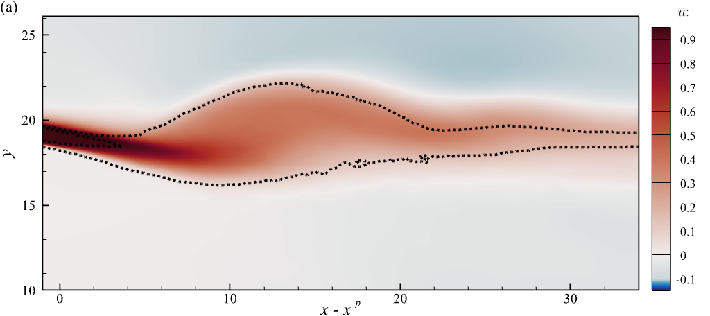
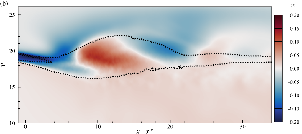
Figure 8: Contours of time-averaged velocities at the mid span: (a), $\overline{u}$; (b), $\overline{v}$. Dotted lines represent the edge of the mixed-phase region. ($\text{Re}=1600$ and $\text{Fr}=6.4$)

Figure 8 shows the contours of mean streamwise and vertical velocities at the mid span for case 6 at an intermediate Froude number $\text{Fr}=6.4$. The dotted lines shows the upper and lower edge of the mixed-phase region. Figure 8(a) shows that the jet plunging induces a mean streamwise velocity $\overline{u}$ near the free surface, and the large magnitude of $\overline{u}$ is collocated with the mixed-phase region. As shown in figure 8(b), the trend of mean vertical velocity $\overline{v}$ varies along the streamwise direction in the mixed-phase region. Near the jet plunging point, the fluid around the jet moves downwards with it. Shortly downstream, the pool water moves upwards, and droplets are generated. Meanwhile, the air cavities under the surface moves upwards under the buoyancy. As a result, the vertical velocity is positive in this region. After the droplets reach the highest, they drop to the pool and form a secondary plunging, which causes another region with negative vertical velocity.

Because the size of mixed-phase region varies in different Froude numbers, to facilitate comparison between results of different cases, we follow Hendrickson and Yue (2019) to define conditioned average in the mixed-phase region as:

$$\left\langle f^{R}\right\rangle_{yz}(x)=\frac{1}{S^{R}(x)}\int_{yz}f^{R}(y,z;x)\mathrm{d}S^{R}.$$ (13)

Here, $f^{R}$ represents the variable $f$ inside the mixed-phase region. The integration denoted by $\left\langle\right\rangle_{yz}$ is performed over a cross-stream section, and $S^{R}(x)$ represents the area of the mixed-phase region in the cross-stream section.

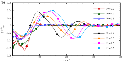
Figure 9: Mean velocities averaged in the mixed-phase region in different Froude numbers: (a), $\left<\overline{u}^{R}\right>_{yz}$; (b), $\left<\overline{v}^{R}\right>_{yz}$.

Figure 9 compares the mean velocities averaged in the mixed-phase region $\left<\overline{u}_{i}^{R}\right>_{yz}$ for different Froude numbers. We note here that the results in the flow region for $x-x^{p}=0.0\sim 4.0$ show some uncertainty, because the area of mixed-phase region $S^{R}(x)$ is small in this flow region. The reliability of statistics is questionable because of the small sampling number. Therefore, in the following content, we mainly focus on the rest flow region for $x-x^{p}>4.0$, where the sampling number is sufficiently large to provide more reliable statistics. This does not influence our understanding of the statistical properties of the mixed-phase turbulence induced by the plunging jet, because active turbulence mainly occurs downstream, where air and water are sufficiently mixed.

Figure 9(a) shows that, as the value of velocity is non-dimensionalized by the jet horizontal velocity, $\left<\overline{u}^{R}\right>_{yz}$ shows little difference near the jet plunging region ($x-x^{p}=4.0\sim 8.0$) at different Froude numbers. This indicates that the mean flow is mainly induced by jet plunging, while turbulent motion does not impose significant influence on the mean flow in this region. Around $x-x^{p}=10.0$, where the splash is intense, the magnitude of $\left<\overline{u}^{R}\right>_{yz}$ reaches a valley. Downstream, $\left<\overline{u}^{R}\right>_{yz}$ shows a non-monotonic response to the increase of the Froude number. At lower Froude numbers ($\text{Fr}\leq 5.3$),$\left<\overline{u}^{R}\right>_{yz}$ increases with the Froude number. For $\text{Fr}\geq 6.4$, there exists intense vertical motion that expands the size of mixed-phase region, and as a result, the streamwise momentum is diffused and $\left<\overline{u}^{R}\right>_{yz}$ decreases as the Froude number increases.

From figure 9(b), it is observed that the magnitude of the first negative peak of $\left<\overline{v}^{R}\right>_{yz}$ around $x-x^{p}=4.0$ decreases as the Froude number increases because of the reduction of the gravitational potential energy of the injected water, which is proportional to $1/\text{Fr}$. Downstream of the plunging region, the vertical motion is weak at low Froude number for $\text{Fr}\leq 5.3$, resulting in small magnitude of $\left<\overline{v}^{R}\right>_{yz}$. For $\text{Fr}\geq 6.4$, the water plunging induces a large amount of droplets, which induce the first positive peak of $\left<\overline{v}^{R}\right>_{yz}$. When the droplets reach the highest altitude, the vertical velocity becomes zero, and this is also the location where the size of mixed-phase region reaches the maximum. The secondary negative peak represents downward motion of droplets, which leads to the secondary plunging. Downstream the secondary plunging, there is still small magnitude of $\left<\overline{v}^{R}\right>_{yz}$ at higher Froude numbers. This indicates that the increasing Froude number results in more intense vertical motion of the surface.

To perform statistical study of turbulent properties, an instantaneous variable $f$ is decomposed as $f(x,y,z;t)=\overline{f}(x,y,z)+f^{\prime}(x,y,z;t)$, where $f^{\prime}$ is the fluctuation. The mean momentum equation of incompressible variable-density flow can be expressed as:

$$\frac{\partial(\overline{\rho}\overline{u}_{i})}{\partial t}=C_{i}+G^{p}_{i}+G_{i}+D^{v}_{i}+D^{t}_{i}+A_{i}.$$ (14)

Budget terms on the right-hand side of equation (14) include the convection term $C_{i}$, pressure gradient term $G^{p}_{i}$, gravity term $G_{i}$, viscous diffusion term $D^{v}_{i}$, Reynolds stress term $D^{t}_{i}$, and TMF term $A_{i}$. These terms are defined as

$$C_{i}=-\frac{\partial\left(\overline{\rho}\overline{u}_{i}\overline{u}_{j}\right)}{\partial x_{j}},$$ (15)

$$G^{p}_{i}=-\frac{\partial\overline{P}}{\partial x_{i}},$$ (16)

$$G_{i}=\frac{\overline{\rho}}{\text{Fr}^{2}}\delta_{i2},$$ (17)

$$D^{v}_{i}=\frac{\partial\overline{\tau}_{ij}}{\partial x_{j}},$$ (18)

$$D^{t}_{i}=-\frac{\partial\overline{\rho u_{i}^{\prime}u_{j}^{\prime}}}{\partial x_{j}},$$ (19)

$$A_{i}=-\frac{\partial\overline{\rho u_{i}^{\prime}}}{\partial t}-\frac{\partial}{\partial x_{j}}\left(\overline{\rho u_{i}^{\prime}}\overline{u}_{j}+\overline{\rho u_{j}^{\prime}}\overline{u}_{i}\right),$$ (20)

where $\tau_{ij}=\mu\left(u_{i,j}+u_{j,i}\right)/\text{Re}$ is the viscous stress tensor. There are unclosed terms on the right hand side of equation (14), namely the Reynolds stress $\overline{\rho u_{i}^{\prime}u_{j}^{\prime}}$ and TMF $\overline{\rho u_{i}^{\prime}}$.

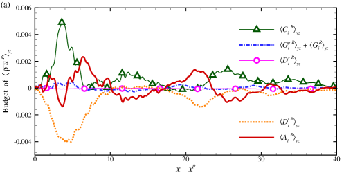
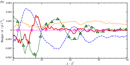
Figure 10: Curves of mixed-phase-region-averaged terms in the right hand side of equation (14) along the streamwise direction. ($\text{Re}=1600$ and $\text{Fr}=6.4$)

Figure 10 shows the averaged value of each budget term of equation (14) in the mixed-phase region. As shown in figure 10(a), the convection term $C_{1}$, Reynolds stress term $D_{1}^{t}$ and TMF term $A_{1}$ make dominant contribution to the transport of $\overline{\rho}\overline{u}$. The convection term $C_{1}$ and Reynolds stress term $D_{1}^{t}$ balance with each other near the jet plunging point. They decay downstream and the TMF term $A_{1}$ becomes a dominant term. Among the budget terms of $\overline{\rho}\overline{v}$, the summation of the gravity term $G_{2}$ and mean pressure gradient term $G^{p}$ make significant contribution. It shows consistency with the variation of the mean vertical velocity along the streamwise direction. The TMF term $A_{2}$ is important near the jet plunging point and decays to a small magnitude for $x-x^{p}\geq 10.0$. The Reynolds stress term $D_{2}^{t}$ plays an important role for $x-x^{p}\geq 10.0$. The results shown in figure 10 indicate that the closure of both Reynolds stress and TMF is important in the mixed-phase turbulence induced by jet plunging.

3.5 Turbulent kinetic energy

There are different strategies for closing the Reynolds stress $\overline{\rho u_{i}^{\prime}u_{j}^{\prime}}$. In the single-phase flows, an important strategy is to use the dynamic equation of TKE $k=\frac{1}{2}\overline{\rho u_{i}^{\prime}u_{i}^{\prime}}$ for closure, such as the $k$–$\varepsilon$ Model (Chien, 1982, Kaul, 2010, 2011) and $k$–$\omega$ model (Wilcox, 1988, Menter, 1994, Spalart and Rumsey, 2007, Wilcox, 2008). In the following context, we first analyse the effect of the Froude number on the TKE, followed by some discussions on if the closure model of TKE in single-phase turbulence can be applied to a mixed-phase turbulent flow.

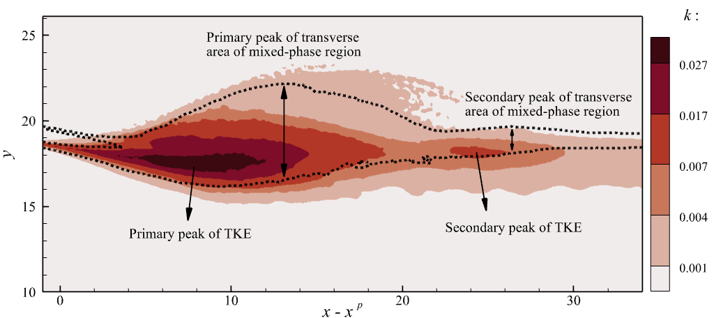
Figure 11: Contours of TKE at the mid span. Dotted line represents the edge of the mixed-phase region. ($\text{Re}=1600$ and $\text{Fr}=6.4$)

Figure 11 displays the contours of TKE at the mid span for $\text{Fr}=6.4$. The figure demonstrates a strong correlation between the mixed-phase region and large magnitude of TKE. The highest TKE is observed below the mean surface downstream near the jet plunging point ($x-x^{p}=4.0\sim 12.0$), where the shear between the jet and the pool water is strong. At approximately $x-x^{p}=24.0$, there is a secondary peak of TKE caused by the secondary plunging.

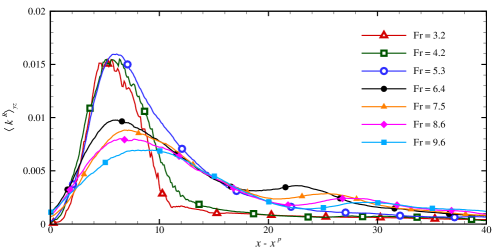
Figure 12: Profiles of average TKE in the mixed-phase region along the streamwise direction in cases of different Froude number.

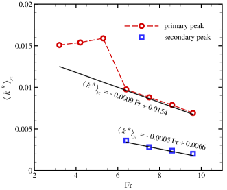
Figure 13: Primary peak (red circle symbols) and secondary peak (blue square symbols) variables of the average TKE in varying with Froude number and the fit curve.

Figure 12 compares the streamwise variation of the TKE averaged in the mixed-phase region $\left\langle k^{R}\right\rangle_{yz}$ for different Froude numbers. At all Froude numbers, a primary peak occurs around $x-x^{p}=6.0$. For large Froude numbers ($\text{Fr}\geq 6.4$), a secondary peak of TKE occurs. Figure 13 compares the magnitudes of the two peaks at different Froude numbers. It is seen that at low Froude numbers, the magnitude of the primary peak increases with Froude number. As the Froude number increases to $\text{Fr}\geq 6.4$, the magnitudes of both primary and secondary peak decrease linearly with the Froude number. The observations from figure 13 indicates that the Froude number imposes dual effects on TKE. At low Froude numbers, the entrained air volume increases and the shear is enhanced near the interface as the Froude number increases. As a result, the magnitude of TKE increases with Froude number ($\text{Fr}\leq 5.3$). At larger Froude numbers ($\text{Fr}\geq 6.4$), the increase in the Froude number leads to the decrease of gravitational potential energy. Consequently, the vertical velocity and the plunging angle decrease when the jet hits the free surface. Furthermore, at higher Froude numbers, more droplets are generated, resulting in secondary plunging. In other words, the TKE is distributed in a wider streamwise range at higher Froude numbers, resulting in a smaller peak value.

The transport equation of TKE in variable-density flows is expressed as  (Chassaing et al., 2002)

$$\frac{\partial k}{\partial t}=C+D^{t}+P+D^{p}+D^{v}+\varepsilon+A.$$ (21)

Budget terms on the right-hand side of equation (21) include the convection term $C$, turbulence-diffusion term $D^{t}$, production term $P$, pressure-diffusion term $D^{p}$, viscous diffusion term $D^{v}$, dissipation term $\varepsilon$, and the TMF-correlation term $A$, defined as

$$C=-\frac{\partial\left(k\overline{u}_{j}\right)}{\partial x_{j}},$$ (22)

$$D^{t}=-\frac{\partial\left(\frac{1}{2}\overline{\rho u_{i}^{\prime}u_{i}^{\prime}u_{j}^{\prime}}\right)}{\partial x_{j}},$$ (23)

$$P=\overline{\rho u_{i}^{\prime}u_{j}^{\prime}}\frac{\partial\overline{u}_{i}}{\partial x_{j}},$$ (24)

$$D^{p}=-\frac{\partial\overline{p^{\prime}u_{i}^{\prime}}}{\partial x_{i}},$$ (25)

$$D^{v}=\frac{\partial\overline{\tau_{ij}^{\prime}u_{i}^{\prime}}}{\partial x_{j}},$$ (26)

$$\varepsilon=-\overline{\tau_{ij}^{\prime}\frac{\partial u_{i}^{\prime}}{\partial x_{j}}},$$ (27)

$$A=\frac{\overline{\rho u_{i}^{\prime}}}{\text{Fr}^{2}}\delta_{i2}-\overline{\rho u_{i}^{\prime}}\left(\frac{\partial\overline{u}_{i}}{\partial t}+\overline{u}_{j}\frac{\partial\overline{u}_{i}}{\partial x_{j}}\right).$$ (28)

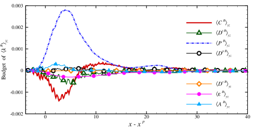
Figure 14: Streamwise variation of the budget terms in transport equation of TKE averaged in the mixed-phase region for $\text{Re}=1600$ and $\text{Fr}=6.4$.

Figure 14 shows the streamwise variation of the budget terms of $\left\langle k^{R}\right\rangle_{yz}$, TKE averaged in cross-stream plane inside the mixed-phase region. The results for $\text{Re}=1600$ and $\text{Fr}=6.4$ are shown. Similar to many single-phase flows, the balance between the production term $P$ and the dissipation term $\varepsilon$ dominates the transport of TKE. The convection term $C$ is positive upstream and changes its sign to negative downstream, indicating energy convection from upstream to downstream. The magnitude of the TMF-correlation term $A$ is smaller than the production term $P$. This indicates that the closure model of single-phase turbulence can be referenced by the mixed-phase turbulence induced by an plunging jet.

3.6 Turbulent mass flux and its transports

Equations (14)–(20) show that there are two unclosed terms in the mean momentum equation of the mixed-phase turbulence. The first term is Reynolds stress tensor and it is usual to consider its isotropic part TKE for closure problems. Analysis of TKE transport equation shows that its budget remains similar to most single-phase turbulent flows. The energy generated by the TMF-correlation term is relatively small, as such the single-phase flow closure model can be used. However, 3.4 shows that the TMF term plays an important role in the transport of mean momentum. Therefore, its closure model is also important for industrial applications. Hendrickson and Yue (2019) developed an algebraic model for TMF based on their iLES data of the wake of a three-dimensional dry transom stern. Their a priori tests showed that it is challenging to obtain an ideal correlation between the model and iLES data. Another strategy to close the TMF is to develop a dynamic model, which requires an analysis of its transport equation. In this section, we investigate the Froude number effects on the TMF, and the transports of TMF is then analysed.

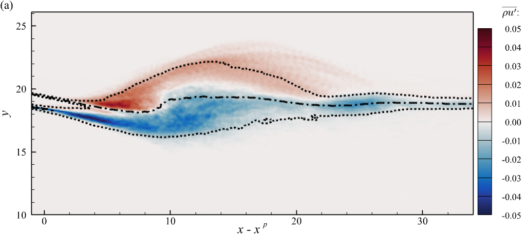
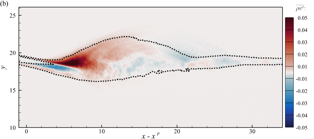
Figure 15: Contours of TMF: (a) $\overline{\rho u^{\prime}}$; (b) $\overline{\rho v^{\prime}}$ at the mid span for $\text{Re}=1600$ and $\text{Fr}=6.4$. The upper and lower dotted lines represent the edge of the mixed-phase region. The dash-dotted line in (a) represents the mean location of free surface.

Figures 15(a) and (b) show the contours of $\overline{\rho u^{\prime}}$ and $\overline{\rho v^{\prime}}$, respectively, at the mid span for $\text{Re}=1600$ and $\text{Fr}=6.4$. The upper and lower dotted lines represent the edge of the mixed-phase region. The dash-dotted line in figure 15(a) represents the mean location of free surface corresponding to $\overline{\psi}=0.5$. As shown in figure 15(a), $\overline{\rho u^{\prime}}$ is positive above the mean free surface, indicating the downstream transport of water droplets. Below the mean free surface, $\overline{\rho u^{\prime}}$ is negatively valued, corresponding to the downstream transport of bubbles. From figure 15(b), it is observed that near both the primary and secondary plunging point, $\overline{\rho v^{\prime}}$ is positive, indicating the air entrainment. Shortly downstream the plunging points, $\overline{\rho v^{\prime}}$ changes its sign to negative, indicating the bubbles detrainment.

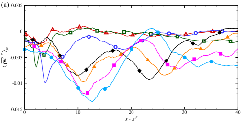
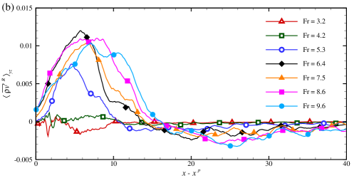
Figure 16: Profiles of TMF averaged in the mixed-phase region along the streamwise direction in cases of different Froude number: (a) $\overline{\rho u^{\prime}}$, (b) $\overline{\rho v^{\prime}}$.

Figure 16 compares the streamwise variation of the TMF averaged in the mixed-phase region for different Froude numbers. Figure 16(a) shows that the negative value of $\overline{\rho u^{\prime}}$ dominates in the mixed-phase region. Recalling that negative and positive $\overline{\rho u^{\prime}}$ correspond to downstream motion of bubbles and droplets, respectively, the negative value of $\left\langle\overline{\rho u^{\prime}}^{R}\right\rangle_{yz}$ indicates that the downstream transfer of air beneath the free surface is dominant. The primary peak of the negatively-valued $\left\langle\overline{\rho u^{\prime}}^{R}\right\rangle_{yz}$ occurs downstream the plunging point. Its magnitude increases as the Froude number increases. This indicates that more bubbles are convected downstream at higher Froude numbers. When $\text{Fr}\geq 6.4$, there exists a secondary peak in $\left\langle\overline{\rho u^{\prime}}^{R}\right\rangle_{yz}$. However, it shows a different trend of the secondary peak as the Froude number increases. This is because the convection of droplets above the surface balances a part of bubble motion beneath the surface. At large Froude numbers, water splash-up induces droplets resulting in the decrease in the magnitude of the secondary negatively-valued peak of $\left\langle\overline{\rho u^{\prime}}^{R}\right\rangle_{yz}$.

Figure 16(b) shows that $\left\langle\overline{\rho v^{\prime}}^{R}\right\rangle_{yz}$ is positive near the plunging point, indicating air entrainment in this region. The magnitude of $\left\langle\overline{\rho v^{\prime}}^{R}\right\rangle_{yz}$ is small at $\text{Fr}=3.2$ and 4.2. It increases as the Froude number increases from 4.2 to 6.4. As the Froude number continues to increase, its magnitude decreases slightly, but the streamwise range with positive $\left\langle\overline{\rho v^{\prime}}^{R}\right\rangle_{yz}$ increases. This indicates that the air entrainment takes place in a larger streamwise region at a higher Froude number. A negative peak of $\left\langle\overline{\rho v^{\prime}}^{R}\right\rangle_{yz}$ occurs for $\text{Fr}\geq 6.4$, caused by the bubble detrainment after the secondary plunging. The magnitude of this negatively-valued peak of $\left\langle\overline{\rho v^{\prime}}^{R}\right\rangle_{yz}$ increases as the Froude number increases from 6.4 to 9.6, indicating that more bubbles are detrained at higher Froude numbers.

To investigate the closure of TMF, we examine the following transport equation of the TMF:

$$\frac{\partial\overline{\rho u_{i}^{\prime}}}{\partial t}=C_{i}+P^{(1)}_{i}+P^{(2)}_{i}+D_{i}+E_{i}.$$ (29)

The budget terms on the right-hand side include convection term $C_{i}$, production terms $P^{(1)}_{i}$ and $P^{(2)}_{i}$ corresponding to the velocity gradient and density gradient, respectively, turbulent diffusion $D_{i}$, and a combining term $E_{i}$. The definitions of these terms are given as

$$C_{i}=-\frac{\partial\left(\overline{\rho u_{i}^{\prime}}\overline{u}_{j}\right)}{\partial x_{j}},$$ (30)

$$P^{(1)}_{i}=-\overline{\rho u_{j}^{\prime}}\frac{\partial\overline{u}_{i}}{\partial x_{j}},$$ (31)

$$P^{(2)}_{i}=-\overline{u_{i}^{\prime}u_{j}^{\prime}}\frac{\partial\overline{\rho}}{\partial x_{j}},$$ (32)

$$D_{i}=\frac{\partial\overline{\rho}\overline{u_{i}^{\prime}u_{j}^{\prime}}}{\partial x_{j}}-\frac{\partial\overline{\rho u_{i}^{\prime}u_{j}^{\prime}}}{\partial x_{j}},$$ (33)

$$E_{i}=\left(\overline{\rho}\overline{\frac{1}{\rho}\frac{\partial p}{\partial x_{i}}}-\frac{\partial\overline{p}}{\partial x_{i}}\right)+\left(\frac{\partial\overline{\tau}_{ij}}{\partial x_{j}}-\overline{\rho}\overline{\frac{1}{\rho}\frac{\partial\tau_{ij}}{\partial x_{j}}}\right).$$ (34)

It should be noted here that the combining term $E_{i}$ consists of a pressure-gradient part and a viscous-stress part. From its expression, it is understood that this term is essentially the difference between their time-averaged values (i.e. ${\partial\overline{p}}/{\partial x_{i}}$ and ${\partial\overline{\tau}_{ij}}/{\partial x_{j}}$) and their density-weighted time-averaged values (i.e. $\overline{\rho}\overline{{\rho}^{-1}{\partial p}/{\partial x_{i}}}$ and $\overline{\rho}\overline{{\rho}^{-1}{\partial\tau_{ij}}/{\partial x_{j}}}$). To perform the density-weighted time averaging, the instantaneous density needs to be interpolated. Owing to the use of sharp-interface treatment in the present simulation, the instantaneous density $\rho$ varies sharply across the interface. As a result, the interpolation of $\rho$ causes oscillation near the interface, resulting in non-physical values. Therefore, in the present study, the pressure-gradient and viscous-stress terms are combined into one term $E_{i}$, and its value is determined indirectly as the opposite number of the summation of other terms. This treatment is supported by the assumption that ${\partial\overline{\rho u_{i}^{\prime}}}/{\partial t}=0$ is attained, and sufficiently long time duration is used for performing time averaging.

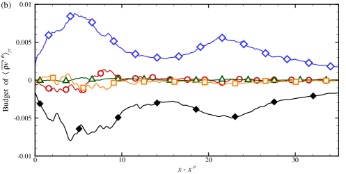
Figure 17: Profiles of average terms on the right-hand side of the TMF (a) $\overline{\rho u^{\prime}}$, (b) $\overline{\rho v^{\prime}}$ transport equation (29) in the mixed-phase region along the streamwise direction. ($\text{Re}=1600$ and $\text{Fr}=6.4$)

Figure 17 shows the streamwise variation of the budget terms of TMF averaged in the mixed-phase region of cross-stream planes. From figure 17(a), it is seen that the budget of $\left\langle\overline{\rho u^{\prime}}^{R}\right\rangle_{yz}$ is influenced by all terms near the jet plunging point. Downstream, convection term $C_{1}$, production term $P^{(1)}_{1}$ and turbulent diffusion term $D_{1}$ decay to a relatively small value, and the budget is mainly balanced by production term $P^{(2)}_{1}$ and combining term $E_{1}$. The balance between production term $P^{(2)}_{2}$ and the combining term $E_{2}$ also dominates the budget of $\left\langle\overline{\rho v^{\prime}}^{R}\right\rangle_{yz}$.

On the right hand side of the transport equation of TMF, the convection term $C_{i}$ and the production term $P^{(1)}_{i}$ do not require modelling. Furthermore, as shown in figure 17, they are not the dominant budget terms. Term $D_{i}$, which can be seen as the diffusion effect of velocity fluctuation on TMF, is only important in the transport of $\left\langle\overline{\rho u^{\prime}}^{R}\right\rangle_{yz}$ near the plunging point, and it can be modelled by estimating a characteristic diffusion velocity using TKE. Term $E_{i}$ is an important transportation term, but due to the lack of reliable data and deeper understanding, it is currently difficult to establish a closure model for this term. Considering the both pressure and viscous stress fluctuations are induced by velocity fluctuations, term $E_{i}$ can be seen as a passive response of the flow field to the change in the other budget terms of the TMF, and can be possibly modelled as a diffusion effect induced by an artificial viscous. Term $P^{(2)}_{i}$ is related to the density gradient caused by two-phase mixture, which is an important production term and can be seen as the direct source term of TMF. Therefore, it is crucial to close term $P^{(2)}_{i}$ in a dynamic model of TMF.

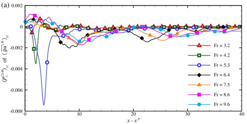
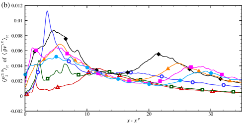
Figure 18: Curves of mean density gradient production term of the TMF (a) $\overline{\rho u^{\prime}}$, (b) $\overline{\rho v^{\prime}}$ averaged in the mixed-phase region along the streamwise direction in different Froude numbers.

Figure 18 compares the streamwise variation of $P^{(2)}_{i}$ averaged in the mixed-phase region in different Froude numbers. At lower Froude numbers ($\text{Fr}\leq 5.3$), $\left\langle P_{1}^{(2)R}\right\rangle_{yz}$ shows a sharp peak near the jet impact point and its absolute value increases with the Froude number. At higher Froude numbers ($\text{Fr}\geq 6.4$), $\left\langle P_{1}^{(2)R}\right\rangle_{yz}$ shows two peaks corresponding to the two plunging events and they both decrease as the Froude number increases. From the comparison between figures 18(a) and 18(b), it is understood that despite of the opposite sign, $\left\langle P_{2}^{(2)R}\right\rangle_{yz}$ is similar to $\left\langle P_{1}^{(2)R}\right\rangle_{yz}$ in terms of both the variation in the streamwise direction and the Froude number effect.

The results of the production term of TMF corresponding to the density gradient displays a better consistency with TKE than TMF. Specifically, there are two peaks of TKE at large Froude numbers ($\text{Fr}\geq 6.4$) and the magnitudes of both peaks decrease as the Froude number increases. Although the TMF also shows two peaks at large Froude numbers ($\text{Fr}\geq 6.4$), their magnitudes show different trends as Froude number increasing. Furthermore, the secondary peak value of $\left\langle\overline{\rho v^{\prime}}^{R}\right\rangle_{yz}$ is negative, while both peaks of $\left\langle P_{2}^{(2)R}\right\rangle_{yz}$ are positive. This indicates that $P_{i}^{(2)}$ can be well modelled by TKE.

Based on the above analyses, we propose a of $P^{(2)}_{i}$ as

$$-\overline{u_{i}^{\prime}u_{j}^{\prime}}\frac{\partial\overline{\rho}}{\partial x_{j}}=-C_{i}\overline{u_{k}^{\prime}u_{k}^{\prime}}\frac{\partial\overline{\rho}}{\partial x_{i}},$$ (35)

where $C_{i}$ is the model coefficients. A linear-least squares fit between $-\overline{u_{i}^{\prime}u_{j}^{\prime}}\frac{\partial\overline{\rho}}{\partial x_{j}}$ and $-\overline{u_{k}^{\prime}u_{k}^{\prime}}\frac{\partial\overline{\rho}}{\partial x_{i}}$ in the mixed-phase region is used to determine the model coefficient. Model coefficients and conditioned correlation coefficients $R_{i}$ between the two sides of equation (35) at different Froude numbers are listed in table 2. Coefficients of streamwise and vertical components of equation (35) are displayed while the spanwise component is not shown because the spanwise component of TMF is much smaller than the other two components. Correlation coefficient of the vertical component exceeds 0.85 and the model coefficient $C_{2}$ vary little with the Froude number. This indicates that $P_{2}^{(2)}$ can be well estimated by the proposed model. Although the accuracy of the streamwise component estimated by the model is not as good as the vertical component, correlation coefficients of the streamwise component are all above 0.55, which is overall higher than the correlation coefficient of the model directly fitting TMF using TKE in Hendrickson and Yue (2019).

Table 2: Model coefficient in equation (35) and conditioned correlation coefficient between the two sides of equation (35) in the mixed-phase region. Two columns of $C_{i}$ and $R_{i}$ indicate the streamwise and vertical components of equation (35) respectively.

case		Fr			$C_{1}$		$R_{1}$			$C_{2}$		$R_{2}$
3		3.2			0.49		0.67			0.30		0.91
4		4.2			0.60		0.56			0.33		0.87
5		5.3			0.58		0.79			0.35		0.96
6		6.4			0.32		0.56			0.35		0.92
7		7.5			0.39		0.69			0.33		0.93
8		8.6			0.46		0.75			0.33		0.95
9		9.6			0.45		0.75			0.32		0.94

4 Conclusion

In the present study, we preformed high-resolution interface-resolved LES to study the mixed-phase turbulence induced by a water jet plunging into a quiescent pool. In total nine cases were conducted. The Reynolds number ranged from $1.6\times 10^{3}$ to $1.6\times 10^{5}$ and the Froude number ranged from $3.2$ to $9.6$ in these cases. By comparing the results of different cases, it was discovered that the effect of the Reynolds number on turbulent statistics was less significant than the Froude number. As a result, this paper mainly focused on the effects of the Froude number on turbulent statistics. The simulation results showed that increasing the Froude number led to the increase in the area of the mixed-phase region. To facilitate comparison among results of different cases, a conditioned average over the cross-sectional area inside the mixed-phase region was adopted.

The mean velocity averaged in the mixed-phase region varies non-monotonically with the Froude number. As the Froude number increases for 3.2 to 9.6, the magnitude of the mean streamwise velocity reaches its maximum at $Fr=6.4$. The mean vertical velocity shows a single negatively-valued peak for low Froude numbers. As the Froude number increases to $Fr\geq 6.4$, water splash-up and secondary plunging take place, causing respectively a positively valued peak and a secondary negatively valued peak in the mean vertical velocity along the streamwise direction. The complex behaviour of the mean velocity is correlated to the nonlinear effects corresponding to the turbulent fluctuation. In mixed-phase turbulence, there exist two unclosed terms in the Reynolds-averaged mean momentum equation, called the Reynolds stress $\overline{\rho u_{i}^{\prime}u_{j}^{\prime}}$ and turbulent mass flux $\overline{\rho u_{i}^{\prime}}$. The analysis of the mean momentum equation showed that both the Reynolds stress and turbulent mass flux are important terms that require closure models.

To discuss the closure problem of the Reynolds-averaged mean momentum equation, we analysed the TKE, TMF and their transport equations. Our simulations showed that the TKE also varies non-monotonically with an increasing Froude number. At low Froude numbers, the TKE shows a singly peak near the plunging point. The magnitude of this TKE peak increases as the Froude number increases from 3.2 to 5.3. As the Froude number increases to $Fr\geq 6.4$, the secondary plunging induces a secondary peak in the TKE. The magnitudes of both primary and secondary peaks of the TKE decreases as the Froude increases from 6.4 to 9.6. The analysis of the transport equation of TKE showed that it is dominated by the balance between production and dissipation. The convection and turbulent diffusion is mainly responsible for the spatial transport of TKE. Transports characteristics of TKE indicate that its closure model for single-phase turbulence can be used in the mixed-phase turbulence induced by the plunging jet.

The TMF term is an additional unclosed term in the Reynolds-averaged mean momentum equation of mixed-phase turbulence. Its value is zero in the single-phase region, while in the mixed-phased region. The streamwise component of TMF is positive above the mean water elevation and is negative below the mean water elevation, corresponding to the streamwise convection of droplets in the air and bubbles in the water, respectively. When the streamwise component of TMF is averaged in the mixed-phase region, its value is negative, indicating that the convection of bubbles dominates the TMF in the streamwise direction. As the Froude number increases, the magnitude of the streamwise component of TMF increases, corresponding to enhanced downstream convection of bubbles. Positive and negative vertical component of TMF occurs alternatively along the streamwise direction. Owing to air entrainment, the vertical component of TMF is positive near the plunging points. In the downstream, the bubbles are detained, causing negative vertical component of TMF. As the Froude number increases, the air entrainment is enhanced. This is characterized by the expansion of the streamwise region with positive vertical TMF. Meanwhile, the air detrainment in the downstream is also enhanced as reflected by the increase in the negative peak of the vertical TMF. In a further analysis of the transport equation of TMF, it is discovered that the production term corresponding to the density gradient shows consistency with the TKE. Based on this finding, a model of this production term is proposed. The a priori test shows satisfactory correlation between the modeled value and the LES data.

To close this paper, we compare the main findings of the present study on the mixed-phase turbulence generated by plunging jet with the results of  Hendrickson and Yue (2019) on the mixed-phase turbulence in a wake flow. The purpose of providing this comparison is to evaluate if the main conclusions of the present study are potentially common for different mixed-phase turbulence, or they are special for the plunging jet. In the present study, it is discovered that the transport of TKE is dominated by the balance between production and dissipation. This is similar to the wake flow. However, the TKE generated by TMF shows less significance in the plunging jet than in the wake flow. As pointed out by Hendrickson and Yue (2019), the model of TMF is needed to close the TKE transport equation. In terms of the closure model of the TMF, the results of both present study and  Hendrickson and Yue (2019) showed that the correlation between TMF and TKE is not strong. Based on this point, we further investigated the transport equation of TMF. We observed that the production term of TMF is in good agreement with TKE. This is a new finding of the present study, leading to a closure model of the production term of TMF, which is potentially useful for future development of a dynamic model of TMF.

References

- Arrufat et al. (2018) T. Arrufat, M. Crialesi-Esposito, D. Fuster, Y. Ling, L. Malan, S. Pal, R. Scardovelli, G. Tryggvason, and S. Zaleski. A mass-momentum consistent, Volume-of-Fluid method for incompressible flow on staggered grids. Computers & Fluids, 215:104785, Jan. 2018. ISSN 00457930. doi: 10.1016/j.compfluid.2020.104785.
- Banner and Peirson (2007) M. L. Banner and W. L. Peirson. Wave breaking onset and strength for two-dimensional deep-water wave groups. Journal of Fluid Mechanics, 585:93–115, Aug. 2007. ISSN 0022-1120, 1469-7645. doi: 10.1017/S0022112007006568.
- Biń (1993) A. K. Biń. Gas entrainment by plunging liquid jets. Chemical Engineering Science, 48(21):3585–3630, 1993. ISSN 0009-2509. doi: 10.1016/0009-2509(93)81019-R.
- Brocchini and Peregrine (2001) M. Brocchini and D. H. Peregrine. The dynamics of strong turbulence at free surfaces. Part 1. Description. Journal of Fluid Mechanics, 449:225–254, Dec. 2001. ISSN 0022-1120, 1469-7645. doi: 10.1017/S0022112001006012.
- Chachereau and Chanson (2011) Y. Chachereau and H. Chanson. Free-surface fluctuations and turbulence in hydraulic jumps. Experimental Thermal and Fluid Science, 35(6):896–909, 2011. ISSN 0894-1777. doi: https://doi.org/10.1016/j.expthermflusci.2011.01.009.
- Chan et al. (2021) W. H. R. Chan, P. L. Johnson, P. Moin, and J. Urzay. The turbulent bubble break-up cascade. Part 2. Numerical simulations of breaking waves. Journal of Fluid Mechanics, 912:A43, Apr. 2021. ISSN 0022-1120, 1469-7645. doi: 10.1017/jfm.2020.1084.
- Chassaing (2001) P. Chassaing. The Modeling of Variable Density Turbulent Flows. A review of first-order closure schemes. Flow, Turbulence and Combustion, 66(4):293–332, July 2001. ISSN 1573-1987. doi: 10.1023/A:1013533322651.
- Chassaing et al. (2002) P. Chassaing, R. A. Antonia, F. Anselmet, L. Joly, and S. Sarkar. Variable Density Fluid Turbulence, volume 69 of Fluid Mechanics and Its Applications. Springer Netherlands, Dordrecht, 2002. ISBN 978-90-481-6040-2 978-94-017-0075-7. doi: 10.1007/978-94-017-0075-7.
- Chen et al. (1999) G. Chen, C. Kharif, S. Zaleski, and J. Li. Two-dimensional Navier–Stokes simulation of breaking waves. Physics of Fluids, 11(1):121–133, Jan. 1999. ISSN 1070-6631, 1089-7666. doi: 10.1063/1.869907.
- Chien (1982) K.-Y. Chien. Predictions of Channel and Boundary-Layer Flows with a Low-Reynolds-Number Turbulence Model. AIAA Journal, 20(1):33–38, Jan. 1982. ISSN 0001-1452, 1533-385X. doi: 10.2514/3.51043.
- Chirichella et al. (2002a) D. Chirichella, R. Gomez Ledesma, K. T. Kiger, and J. H. Duncan. Incipient air entrainment in a translating axisymmetric plunging laminar jet. Physics of Fluids, 14(2):781–790, Feb. 2002a. ISSN 1070-6631, 1089-7666. doi: 10.1063/1.1433493.
- Chirichella et al. (2002b) D. Chirichella, R. Gomez Ledesma, K. T. Kiger, and J. H. Duncan. Incipient air entrainment in a translating axisymmetric plunging laminar jet. Physics of Fluids, 14(2):781–790, Feb. 2002b. ISSN 1070-6631, 1089-7666. doi: 10.1063/1.1433493.
- Clanet and Lasheras (1997) C. Clanet and J. C. Lasheras. Depth of penetration of bubbles entrained by a plunging water jet. Physics of Fluids, 9(7):1864–1866, July 1997. ISSN 1070-6631, 1089-7666. doi: 10.1063/1.869336.
- Deane and Stokes (2002) G. Deane and M. Stokes. Scale dependence of bubble creation mechanisms in breaking waves. Nature, 418(6900):839–844, 2002. doi: 10.1038/nature00967.
- Deike (2022) L. Deike. Mass Transfer at the Ocean–Atmosphere Interface: The Role of Wave Breaking, Droplets, and Bubbles. Annual Review of Fluid Mechanics, 54(1):191–224, Jan. 2022. ISSN 0066-4189, 1545-4479. doi: 10.1146/annurev-fluid-030121-014132.
- Deike et al. (2015) L. Deike, S. Popinet, and W. K. Melville. Capillary effects on wave breaking. Journal of Fluid Mechanics, 769:541–569, Apr. 2015. ISSN 0022-1120, 1469-7645. doi: 10.1017/jfm.2015.103.
- Deike et al. (2016a) L. Deike, W. K. Melville, and S. Popinet. Air entrainment and bubble statistics in breaking waves. Journal of Fluid Mechanics, 801:91–129, Aug. 2016a. ISSN 0022-1120, 1469-7645. doi: 10.1017/jfm.2016.372.
- Deike et al. (2016b) L. Deike, W. K. Melville, and S. Popinet. Air entrainment and bubble statistics in breaking waves. Journal of Fluid Mechanics, 801:91–129, 2016b. doi: 10.1017/jfm.2016.372.
- Delacroix et al. (2016) S. Delacroix, G. Germain, B. Gaurier, and J.-Y. Billard. Experimental study of bubble sweep-down in wave and current circulating tank: Part I—Experimental set-up and observed phenomena. Ocean Engineering, 120:78–87, July 2016. ISSN 00298018. doi: 10.1016/j.oceaneng.2016.05.003.
- Derakhti and Kirby (2016) M. Derakhti and J. T. Kirby. Breaking-onset, energy and momentum flux in unsteady focused wave packets. Journal of Fluid Mechanics, 790:553–581, Mar. 2016. ISSN 0022-1120, 1469-7645. doi: 10.1017/jfm.2016.17.
- Deshpande and Trujillo (2013) S. S. Deshpande and M. F. Trujillo. Distinguishing features of shallow angle plunging jets. Physics of Fluids, 25(8):082103, Aug. 2013. ISSN 1070-6631, 1089-7666. doi: 10.1063/1.4817389.
- Deshpande et al. (2012) S. S. Deshpande, M. F. Trujillo, X. Wu, and G. Chahine. Computational and experimental characterization of a liquid jet plunging into a quiescent pool at shallow inclination. International Journal of Heat and Fluid Flow, 34:1–14, Apr. 2012. ISSN 0142727X. doi: 10.1016/j.ijheatfluidflow.2012.01.011.
- Drazen et al. (2008) D. A. Drazen, W. K. Melville, and L. Lenain. Inertial scaling of dissipation in unsteady breaking waves. Journal of Fluid Mechanics, 611:307–332, Sept. 2008. ISSN 0022-1120, 1469-7645. doi: 10.1017/S0022112008002826.
- Eggers (2001) J. Eggers. Air Entrainment through Free-Surface Cusps. Physical Review Letters, 86(19):4290–4293, May 2001. ISSN 0031-9007, 1079-7114. doi: 10.1103/PhysRevLett.86.4290.
- El Hammoumi et al. (2002) M. El Hammoumi, J. L. Achard, and L. Davoust. Measurements of air entrainment by vertical plunging liquid jets. Experiments in Fluids, 32(6):624–638, June 2002. ISSN 0723-4864, 1432-1114. doi: 10.1007/s00348-001-0388-1.
- Garrett et al. (2000) C. Garrett, M. Li, and D. Farmer. The Connection between Bubble Size Spectra and Energy Dissipation Rates in the Upper Ocean. Journal of Physical Oceanography, 30(9):2163–2171, Sept. 2000. ISSN 0022-3670, 1520-0485. doi: 10.1175/1520-0485(2000)030¡2163:TCBBSS¿2.0.CO;2.
- Grasso and Speziale (1989) F. Grasso and C. Speziale. Supersonic flow computations by two-equation turbulence modeling. In 9th Computational Fluid Dynamics Conference, Buffalo,NY,U.S.A., June 1989. American Institute of Aeronautics and Astronautics. doi: 10.2514/6.1989-1951.
- Hendrickson and Yue (2019) K. Hendrickson and D. K.-P. Yue. Wake behind a three-dimensional dry transom stern. Part 2. Analysis and modelling of incompressible highly variable density turbulence. Journal of Fluid Mechanics, 875:884–913, Sept. 2019. ISSN 0022-1120, 1469-7645. doi: 10.1017/jfm.2019.506.
- Hendrickson et al. (2019) K. Hendrickson, G. D. Weymouth, X. Yu, and D. K.-P. Yue. Wake behind a three-dimensional dry transom stern. Part 1. Flow structure and large-scale air entrainment. Journal of Fluid Mechanics, 875:854–883, Sept. 2019. ISSN 0022-1120, 1469-7645. doi: 10.1017/jfm.2019.505.
- Hsiao et al. (2013) C.-T. Hsiao, X. Wu, J. Ma, and G. Chahine. Numerical and experimental study of bubble entrainment due to a horizontal plunging jet. International Shipbuilding Progress, 60(1-4):435–469, 2013. doi: 10.3233/ISP-130093.
- Iafrati (2009) A. Iafrati. Numerical study of the effects of the breaking intensity on wave breaking flows. Journal of Fluid Mechanics, 622:371–411, Mar. 2009. ISSN 0022-1120, 1469-7645. doi: 10.1017/S0022112008005302.
- Jeong and Moffatt (1992) J.-T. Jeong and H. K. Moffatt. Free-surface cusps associated with flow at low Reynolds number. Journal of Fluid Mechanics, 241:1–22, Aug. 1992. ISSN 0022-1120, 1469-7645. doi: 10.1017/S0022112092001927.
- Jones (1979) W. P. Jones. Models for turbulent flows with variable density and combustion. In Von Karman Inst. for Fluid Dyn. Prediction Methods for Turbulent Flows 37 p (SEE N80-12317 03-34), Jan. 1979.
- Joseph et al. (1991) D. D. Joseph, J. Nelson, M. Renardy, and Y. Renardy. Two-dimensional cusped interfaces. Journal of Fluid Mechanics, 223(-1):383, Feb. 1991. ISSN 0022-1120, 1469-7645. doi: 10.1017/S0022112091001477.
- Kaul (2010) U. Kaul. Effect of Inflow Boundary Conditions on the Solution of Transport Equations for Internal Flows. In 40th Fluid Dynamics Conference and Exhibit, Chicago, Illinois, June 2010. American Institute of Aeronautics and Astronautics. ISBN 978-1-60086-956-3. doi: 10.2514/6.2010-4743.
- Kaul (2011) U. K. Kaul. Effect of Inflow Boundary Conditions on the Turbulence Solution in Internal Flows. AIAA Journal, 49(2):426–432, Feb. 2011. ISSN 0001-1452, 1533-385X. doi: 10.2514/1.J050532.
- Kiger and Duncan (2012) K. T. Kiger and J. H. Duncan. Air-Entrainment Mechanisms in Plunging Jets and Breaking Waves. Annual Review of Fluid Mechanics, 44(1):563–596, Jan. 2012. ISSN 0066-4189, 1545-4479. doi: 10.1146/annurev-fluid-122109-160724.
- Lin and Reitz (1998) S. P. Lin and R. D. Reitz. DROP AND SPRAY FORMATION FROM A LIQUID JET. Annual Review of Fluid Mechanics, 30(1):85–105, Jan. 1998. ISSN 0066-4189, 1545-4479. doi: 10.1146/annurev.fluid.30.1.85.
- Lorenceau et al. (2003) É. Lorenceau, F. Restagno, and D. Quéré. Fracture of a Viscous Liquid. Physical Review Letters, 90(18):184501, May 2003. ISSN 0031-9007, 1079-7114. doi: 10.1103/PhysRevLett.90.184501.
- Lorenceau et al. (2004) É. Lorenceau, D. Quéré, and J. Eggers. Air Entrainment by a Viscous Jet Plunging into a Bath. Physical Review Letters, 93(25):254501, Dec. 2004. ISSN 0031-9007, 1079-7114. doi: 10.1103/PhysRevLett.93.254501.
- Lubin and Glockner (2015) P. Lubin and S. Glockner. Numerical simulations of three-dimensional plunging breaking waves: Generation and evolution of aerated vortex filaments. Journal of Fluid Mechanics, 767:364–393, Mar. 2015. ISSN 0022-1120, 1469-7645. doi: 10.1017/jfm.2015.62.
- Ma et al. (2011) J. Ma, A. A. Oberai, D. A. Drew, R. T. Lahey, and M. C. Hyman. A Comprehensive Sub-Grid Air Entrainment Model for RaNS Modeling of Free-Surface Bubbly Flows. The Journal of Computational Multiphase Flows, 3(1):41–56, Mar. 2011. ISSN 1757-482X, 1757-4838. doi: 10.1260/1757-482X.3.1.41.
- McKeogh and Ervine (1981) E. McKeogh and D. Ervine. Air entrainment rate and diffusion pattern of plunging liquid jets. Chemical Engineering Science, 36(7):1161–1172, 1981. ISSN 0009-2509. doi: 10.1016/0009-2509(81)85064-6.
- Melville (1994) W. K. Melville. Energy dissipation by breaking waves. Journal of Physical Oceanography, 24(10):2041–2049, 1994. doi: 10.1175/1520-0485(1994)024¡2041:EDBBW¿2.0.CO;2.
- Melville et al. (2002) W. K. Melville, F. Veron, and C. J. White. The velocity field under breaking waves: Coherent structures and turbulence. Journal of Fluid Mechanics, 454:203–233, Mar. 2002. ISSN 0022-1120, 1469-7645. doi: 10.1017/S0022112001007078.
- Menter (1994) F. R. Menter. Two-equation eddy-viscosity turbulence models for engineering applications. AIAA Journal, 32(8):1598–1605, Aug. 1994. ISSN 0001-1452, 1533-385X. doi: 10.2514/3.12149.
- Mostert et al. (2022) W. Mostert, S. Popinet, and L. Deike. High-resolution direct simulation of deep water breaking waves: Transition to turbulence, bubbles and droplets production. Journal of Fluid Mechanics, 942:A27, July 2022. ISSN 0022-1120, 1469-7645. doi: 10.1017/jfm.2022.330.
- Nangia et al. (2019) N. Nangia, B. E. Griffith, N. A. Patankar, and A. P. S. Bhalla. A robust incompressible Navier-Stokes solver for high density ratio multiphase flows. Journal of Computational Physics, 390:548–594, Aug. 2019. ISSN 00219991. doi: 10.1016/j.jcp.2019.03.042.
- Nichols (1990) R. H. Nichols. A two-equation model for compressible flows. In AIAA, Aerospace Sciences Meeting, Jan. 1990.
- Rapp and Melville (1990) R. J. Rapp and W. K. Melville. Laboratory measurements of deep-water breaking waves. Philosophical Transactions of the Royal Society of London. Series A, Mathematical and Physical Sciences, 331:735–800, 1990.
- Rudman (1998) M. Rudman. A volume-tracking method for incompressible multifluid flows with large density variations. International Journal for Numerical Methods in Fluids, 28(2):357–378, Aug. 1998. ISSN 0271-2091, 1097-0363. doi: 10.1002/(SICI)1097-0363(19980815)28:2¡357::AID-FLD750¿3.0.CO;2-D.
- Samet and Tamminen (1988) H. Samet and M. Tamminen. Efficient component labeling of images of arbitrary dimension represented by linear bintrees. IEEE Transactions on Pattern Analysis and Machine Intelligence, 10(4):579–586, July 1988. ISSN 01628828. doi: 10.1109/34.3918.
- Sene (1988) K. Sene. Air entrainment by plunging jets. Chemical Engineering Science, 43(10):2615–2623, 1988. ISSN 0009-2509. doi: 10.1016/0009-2509(88)80005-8.
- Spalart and Rumsey (2007) P. R. Spalart and C. L. Rumsey. Effective Inflow Conditions for Turbulence Models in Aerodynamic Calculations. AIAA Journal, 45(10):2544–2553, Oct. 2007. ISSN 0001-1452, 1533-385X. doi: 10.2514/1.29373.
- Taulbee and Vanosdol (1991) D. Taulbee and J. Vanosdol. Modeling turbulent compressible flows - The mass fluctuating velocity and squared density. In 29th Aerospace Sciences Meeting, Reno,NV,U.S.A., Jan. 1991. American Institute of Aeronautics and Astronautics. doi: 10.2514/6.1991-524.
- Tian et al. (2010) Z. Tian, M. Perlin, and W. Choi. Energy dissipation in two-dimensional unsteady plunging breakers and an eddy viscosity model. Journal of Fluid Mechanics, 655:217–257, July 2010. ISSN 0022-1120, 1469-7645. doi: 10.1017/S0022112010000832.
- van der Lans et al. (1979) R. van der Lans, J. Donk, and J. Smith. The effect of contaminants with oxygen transfer rate achieved with a plunging jet contactor. volume 1, Apr. 1979.
- Vreman (2004) A. W. Vreman. An eddy-viscosity subgrid-scale model for turbulent shear flow: Algebraic theory and applications. Physics of Fluids, 16(10):3670–3681, 2004. doi: 10.1063/1.1785131.
- Wang et al. (2016a) Z. Wang, J. Yang, and F. Stern. High-fidelity simulations of bubble, droplet and spray formation in breaking waves. Journal of Fluid Mechanics, 792:307–327, Apr. 2016a. ISSN 0022-1120, 1469-7645. doi: 10.1017/jfm.2016.87.
- Wang et al. (2016b) Z. Wang, J. Yang, and F. Stern. High-fidelity simulations of bubble, droplet and spray formation in breaking waves. Journal of Fluid Mechanics, 792:307–327, 2016b. doi: 10.1017/jfm.2016.87.
- Wilcox (1988) D. C. Wilcox. Reassessment of the scale-determining equation for advanced turbulence models. AIAA Journal, 26(11):1299–1310, Nov. 1988. ISSN 0001-1452, 1533-385X. doi: 10.2514/3.10041.
- Wilcox (2008) D. C. Wilcox. Formulation of the k-w Turbulence Model Revisited. AIAA Journal, 46(11):2823–2838, Nov. 2008. ISSN 0001-1452, 1533-385X. doi: 10.2514/1.36541.
- Yang et al. (2018) Z. Yang, B.-Q. Deng, and L. Shen. Direct numerical simulation of wind turbulence over breaking waves. Journal of Fluid Mechanics, 850:120–155, Sept. 2018. ISSN 0022-1120, 1469-7645. doi: 10.1017/jfm.2018.466.
- Yang et al. (2021) Z. Yang, M. Lu, and S. Wang. A robust solver for incompressible high-Reynolds-number two-fluid flows with high density contrast. Journal of Computational Physics, 441:110474, Sept. 2021. ISSN 00219991. doi: 10.1016/j.jcp.2021.110474.
- Yu et al. (2019) X. Yu, K. Hendrickson, B. K. Campbell, and D. K. P. Yue. Numerical investigation of shear-flow free-surface turbulence and air entrainment at large Froude and Weber numbers. Journal of Fluid Mechanics, 880:209–238, Dec. 2019. ISSN 0022-1120, 1469-7645. doi: 10.1017/jfm.2019.695.