Temporal ordering of mixed and noisy data

PCA matrix denoising is uniform

Abstract

Principal component analysis (PCA) is a simple and popular tool for processing high dimensional data. We investigate its effectiveness for matrix denoising. We assume i.i.d. high dimensional Gaussian noises with standard deviation $\sigma$ are added to clean data generated from a low dimensional subspace. We show that the distance between each pair of PCA-denoised data point and the clean data point is uniformly bounded by $\widetilde{O}(\sigma)$, assuming a low-rank data matrix with mild singular value assumptions. We show such a condition could arise even if the data lies on curves. We then provide a general lower bound for the error of the denoised data matrix, which indicates PCA denoising gives a uniform error bound that is rate-optimal. Furthermore, we examine how the error bound impacts downstream applications such as empirical risk minimization, clustering, and manifold learning. Numerical results validate our theoretical findings and reveal the importance of the uniform error.

1 Introduction

In the modern era, data is often referred to as “the new gold”. Rich data with rapidly increasing statistical methods present us with powerful tools for extracting valuable information and explaining scientific problems. However, the process of collecting data inevitably introduces noise, which poses a significant challenge. While statistical methods typically exhibit stability in the presence of weak noise, they may struggle to perform well when the noise surpasses the signal present in clean data. This issue becomes particularly pronounced in the realm of high-dimensional data where each dimension of the data point is corrupted by noise. As the number of dimension grows, the overall noise also grows, which further exacerbate the curse of dimensionality (Donoho et al., 2000) when we try to analyze high-dimensional data given a small number of observations.

Take a case where $n$ clean data points $X_{i}\in\mathbb{R}^{d}$ are corrupted by independent and identically distributed (i.i.d.) Gaussian noise $\xi_{i}\sim\mathcal{N}(0,\sigma^{2}I_{d})$. In other words, what we can observe are the noisy data points $Z_{i}=X_{i}+\xi_{i}$, $i\in[n]$. For simplicity of exposition, we always assume $\|X_{i}\|\leq 1$ without loss of generality for all $i$ throughout this paper. Now, we introduce the signal-to-noise ratio (SNR), which is a standard metric that measures the relative strength of the signal when compared with the noise. In this simple setting, the SNR is given by:

$$\text{SNR}=\frac{\|X_{i}\|^{2}}{\mathbb{E}[\|\xi_{i}\|]^{2}}\leq\frac{1}{\sigma^{2}d}.$$

When we increase the dimensionality $d$, the SNR deteriorates and tends towards zero. With a low SNR, analyzing data directly based on $Z$ will induce unsatisfactory results. Naturally, we seek to denoise $Z$ first to improve the accuracy of data analysis. This procedure is known as matrix denoising in the literature (see for example (Donoho and Gavish, 2014)), and we introduce it in the following section.

1.1 PCA for denoising

Suppose the clean data points $X_{i}$ are distributed in a low-dimensional subspace with a dimension of $r$, where $r\ll d$. A direct idea to recover $X_{i}$ is to use the singular value decomposition (SVD) of the noisy data matrix formed by $Z_{i}$.

Let $X=[X_{1},....,X_{n}]^{T}\in\mathbb{R}^{n\times d}$, where each row represents a clean data point. Similarly, we have the noisy data $Z=[Z_{1},\ldots,Z_{n}]^{T}=X+E$, where the rows of $E$ are $\xi_{i}\sim\mathcal{N}(0,\sigma^{2}I_{d})$. Assuming $X$ is rank$(r)$, let us consider the following hypothetical procedure. Let the SVD of $X$ be denoted as $X=U\Lambda V^{T}$, where $U\in\mathbb{R}^{n\times r}$, $\Lambda\in\mathbb{R}^{r\times r}$, and $V\in\mathbb{R}^{d\times r}$. The columns of $V$ span the subspace in which $X$ lies, with a dimension of $r$ and $VV^{T}$ is the projection operator onto this subspace. By applying this projection operator to $Z_{i}$, we obtain:

$$VV^{T}Z_{i}=X_{i}+VV^{T}\xi_{i},\quad\text{where }\mathbb{E}[\|VV^{T}\xi_{i}\|^{2}]=\sigma^{2}\text{tr}(VV^{T})=r\sigma^{2}.$$

Thus, when the dimension of the subspace, $r$, is fixed and much smaller than $d$, the noise in the projection $VV^{T}Z_{i}$ is significantly weaker than the noise in $Z_{i}$. For the projected data $VV^{T}Z_{i}$, the associated SNR is of order ${1}/{(\sigma^{2}r)}$, which can be sufficiently strong to yield accurate inference results. Therefore, by leveraging the SVD and performing the projection onto the low-dimensional subspace, we can effectively denoise the data and obtain accurate estimates.

In practice, there is no access to $V$. Therefore, we estimate it using the SVD of the noisy data matrix $Z$. The SVD of $Z$ can be expressed as $Z=\hat{U}\hat{\Lambda}\hat{V}^{T}$, where typically $Z$ has full rank due to the presence of noise. To focus on the most significant components of the data, we select only the first $r$ columns of $\hat{V}$, denoted as $\hat{V}_{r}$, corresponding to the largest $r$ singular values. By $\hat{V}_{r}$, we project the noisy data points $Z_{i}$ onto the estimated subspace, resulting in the denoised estimates $\hat{X}_{i}$. The projection is given by:

$$\hat{X}_{i}=\hat{V}_{r}\hat{V}_{r}^{T}Z_{i},\quad i\in[n].$$

The columns of $\hat{V}_{r}$ can be interpreted as the $r$ directions that capture the most variability of the data points $Z_{i}$. Therefore, they are often referred to as the principal directions, and the resulting $\hat{X}_{i}$ are known as the principal components. This approach is commonly known as principal component analysis (PCA). We call it the PCA-denoising algorithm, presented in Table 1.

Utilizing PCA for noise reduction is not a new concept. It was first introduced in multivariate statistical analysis and then explored in various fields. For example, Shepard (1962) introduced the use of PCA for multidimensional scaling and distance estimation. In the field of image processing, Singh and Harrison (1985) applied PCA to denoise images. Discussions in Section 1.3 provide more related literature and results. We also refer interested readers to surveys and textbooks for more comprehensive lists (Jolliffe, 2005; Abdi and Williams, 2010; Chen et al., 2021).

The denoised data $\hat{X}$ can be applied to various applications, such as empirical risk minimization, clustering, manifold learning and so on. The denoising step largely improves the performance of algorithms in these fields. More discussions can be found in our Section 4.

Algorithm 1 PCA-denoising

1:Data $Z\in\mathbb{R}^{n\times d}$, dimension $r$.

2:Denoised data $\hat{X}\in\mathbb{R}^{n\times d}$.

3:Find the SVD of $Z$ as $Z=\hat{U}\hat{\Lambda}\hat{V}^{T}$.

4:Denote the first $r$ columns of $\hat{V}$ as $\hat{V}_{r}\in\mathbb{R}^{d\times r}$.

5:Let $\hat{X}=Z\hat{V}_{r}\hat{V}_{r}^{T}$.

1.2 Our main interest and contribution

One crucial question for matrix denoising is assessing the accuracy of $\hat{X}_{i}$, i.e. the distance between the estimate $\hat{X}_{i}$ and the clean data $X_{i}$ for all $i\in[n]$. Most existing theoretical analysis of PCA focuses on the distance between the two matrices $\hat{X}$ and $X$ as a whole, which can be seen as an “average error”. Our goal is to obtain a uniform error bound across all data points, which allows for individual statistical analysis on each sample. Specifically, we aim to establish the following uniform error bound for the PCA-based denoising algorithm:

$$\|\hat{X}-X\|_{\text{unif}}:=\max_{i\in[n]}\|X_{i}-\hat{X}_{i}\|=\widetilde{O}(\sigma),$$ (1)

with high probability. Here, the notation $\widetilde{O}(\sigma)$ represents an error at the order of at most $\sigma(\log n)^{c}$, where $c>0$ is a constant. Here $\widetilde{O}(\sigma)=O(\sigma(\log n)^{c})$ for some constant $c>0$.

To understand our goal (1), we consider a special case where the observed data $Z_{i}$ also has a dimension of $r$. In this low-dimensional case, the noise $E_{i}$ has a low dimension of $r$ and the dimension reduction is not necessary. One can directly use the observed data $Z_{i}$ as an estimate of the clean data $X_{i}$. According to the random matrix theory (Vershynin, 2010), the estimation error is $\|Z-X\|_{\text{unif}}=\|E\|_{\text{unif}}=\widetilde{O}(\sigma)$, the same as (1). Therefore, our goal (1) implies that the PCA-denoising estimates $\hat{X}_{i}$ achieve the same level of accuracy as in the low-dimensional case. In other words, the PCA-denoising step essentially removes the curse of dimensionality.

In this paper, we explore the estimate (1) from several perspectives. Here is a summary of our main findings:

1. In Section 2.1, Theorem 1 establishes a general form of (1) under the condition $\|X_{i}\|\leq 1$. We then show that when a mild assumption $\lambda_{r}(X)\geq c_{X}\sqrt{n}$ holds, where $\lambda_{r}(X)$ denotes the $r$-th smallest singular value of $X$, the estimate (1) holds exactly. The results hold when $X_{i}$ are non-i.i.d. and have an arbitrary correlation.

2. In Section 2.3, we investigate the sufficient conditions that the assumption $\lambda_{r}(X)\geq c_{X}\sqrt{n}$ holds. By the random matrix theory, we demonstrate that the covariance matrix of $X$ with a non-zero $r$-th eigenvalue will suffice. As an example, we use it to show that $X$ distributed on a zigzag line will meet this assumption.

3. Section 3 presents a general lower bound on the signal-to-noise ratio and sample size $n$ to ensure that the average error is no larger than any constant $\epsilon>0$. The lower bound highlights that PCA-denoising has the optimal noise and sample size requirement.

4. In Section 4, we demonstrate the practical implications of the uniform error bound $\|\hat{X}-X\|_{\text{unif}}$ in various downstream applications. Assuming $\|\hat{X}-X\|_{\text{unif}}\leq\epsilon$, we provide performance guarantees for applications such as empirical risk minimization for supervised learning, clustering, and manifold learning.

5. Finally, in Section 5, we provide some numerical simulations to support our theoretical findings. We consider a clustering task on high-dimensional data sampled from two separated zigzag lines. We show that PCA-denoising of the data yields the uniform error bound (1), and the denoised data enables efficient spectral clustering. We also show that data with a small “average error” alone is not sufficient for achieving good clustering results for every sample in this task.

At last, we want to point out that the uniform error is not a new term. In the statistical literature, it is sometimes referred to as the $2\to\infty$ norm, which is defined by

$$\|\hat{X}-X\|_{2,\infty}=\max_{a\in\mathbb{R}^{d},a\neq 0}\frac{\|(\hat{X}-X)a\|_{\infty}}{\|a\|_{2}}.$$

Their equivalence be found in Cape et al. (2019a, b), which provides further theoretical insights into our results. We call it “the uniform error” throughout this paper to emphasize the intuitive understanding of the concept and its implications.

1.3 Related literature

Our findings reside at the intersection of PCA and matrix denoising, where plenty of related results exist in the literature. In this section, we will provide a brief overview of the relevant literature from the perspectives of PCA and matrix denoising.

1.3.1 Comparing with PCA literature

Due to the wide range of applications for PCA, there is numerous of literature on its design and applications (Abdi and Williams, 2010). The earliest works can be traced back to the 1960s (Rao, 1964; Jolliffe, 1972), where the discussion focus on multivariate statistical analysis. However, a rigorous understanding of PCA in high-dimensional settings emerged much later, mostly in the last 15 years. In the theoretical analysis of PCA, most studies have focused on the accuracy of subspace recovery, i.e. $\|\hat{V}_{r}\hat{V}^{T}_{r}-VV^{T}\|_{*}$. Here $\|\,\cdot\,\|_{*}$ is some operator norm and $\ell_{2}$-operator norm is used in most classical settings. Denote $\mathcal{E}_{V}=\hat{V}_{r}\hat{V}^{T}_{r}-VV^{T}$ for short. Using the eigenvector perturbation results like Davis and Kahan (1970); Wedin (1972); Yu et al. (2015), and random matrix theory, an upper bound of the form $\|\mathcal{E}_{V}\|^{2}\leq O(\sigma^{2}d/n)$ can be obtained, with additional ranks condition (Johnstone and Lu, 2009; Cai and Zhang, 2018; Abbe et al., 2020). Additional conditions can generalize such bounds to $l_{2\to\infty}$ or $l_{\infty}$ norms (Cape et al., 2019b; Fan et al., 2018). In Reiss and Wahl (2020), the error is studied when $VV^{T}$ is replaced by a rank-$r$ projection $P$ that minimizes $\mathbb{E}\|Z-PZ\|^{2}$. In Zhang et al. (2022), the problem is extended to the setting where the data distribution is heteroskedastic.

Using the upper bound on $\|\mathcal{E}_{V}\|$, we can straightforwardly obtain the accuracy of PCA for a new data point. Suppose $X_{n+1}$ is a new data point on the same subspace, and $\xi_{n+1}\sim\mathcal{N}(0,\sigma^{2}I_{d})$. Then the expected error of $\hat{X}_{n+1}=\hat{V}_{r}\hat{V}^{T}_{r}Z_{n+1}$ can be shown to be

$$\mathbb{E}[\|\hat{X}_{n+1}-X_{n+1}\|^{2}]=\mathbb{E}[\|\mathcal{E}_{V}X_{n+1}\|^{2}+\|\hat{V}_{r}\hat{V}^{T}_{r}\xi_{n+1}\|^{2}]=O(\sigma^{2}(d/n+r)).$$

This noise level is the same as our goal in (1). However, in the proof, the independence between $\xi_{n+1}$ and $\hat{V}_{r}$ is used to obtain the bound on $|\hat{V}_{r}\hat{V}^{T}_{r}\xi_{n+1}|^{2}$. Without this independence, such as in the case of $|\hat{V}_{r}\hat{V}^{T}_{r}\xi_{k}|^{2}$ for $k\in[n]$, this bound does not hold. In other words, bounding $\|\mathcal{E}_{V}\|$ does not directly lead to the desired (1).

While this “new data error bound” is already useful in many situations, it imposes constraints in practical applications. To ensure the independence condition between $\hat{V}_{r}$ and the data points to be projected, one has to split the data into two sets: one training data set to obtain the projection $\hat{V}_{r}\hat{V}_{r}^{T}$, and another set where this projection is applied. The “new data error bound” cannot be applied if the projection is on the training data set. This data-splitting approach leads to two problems: 1) It reduces the sample size, resulting in a loss of estimation accuracy, which is undesirable when the original dataset has a limited number of samples. 2) In many unsupervised learning tasks, statistical inference on the training data set itself is crucial. For example, we want to classify all data points in the clustering problem. Yet the clustering error on the training data cannot be evaluated using the “new data error bound”.

In contrast, with a uniform bound of the form (1), the data splitting is no longer necessary. We can obtain $\hat{V}_{r}$ from all samples and apply the projection to all of them. It is more accurate with a larger sample size, and allows us to carry out unsupervised operations on all the samples.

1.3.2 Comparing with matrix denoising literature

In the matrix denoising literature, researchers aim to find an estimate $\hat{X}(Z)$ so that $\|\hat{X}(Z)-X\|$ can be well bounded. Various approaches have been introduced to tackle this problem, including regularization methods (Donoho and Gavish, 2014), shrinkage methods (Nadakuditi, 2014), and online methods (Ding, 2020). Montanari et al. (2018) discusses the implication of finding the optimal $\hat{X}$ in a certain family of matrices, although it does not provide a concrete algorithm to obtain the optimizer. Compared with these methods, the PCA-denoising approach is much simpler, more straightforward, and widely adopted.

Existing analyses of matrix denoising focus on obtaining an error bound of $\|\hat{X}-X\|$ (Donoho and Gavish, 2014; Montanari et al., 2018; Ding, 2020), which is equivalent to an “average denoise error bound”

$$\frac{1}{n}\sum_{i=1}^{n}\|X_{i}-\hat{X}_{i}\|^{2}=O(\sigma^{2}).$$ (2)

This average error is at the same order as the uniform error bound in (1) up to a logarithm term, and later we will discuss the difference between them. Another direction of focus is the subspace recovered as a subsequent result (Ding, 2020; Leeb, 2021; Bao et al., 2021). Results in this direction are similar to those from the PCA literature in Section 1.3.1.

We now compare the “average error bound” with the “uniform error bound” of our interest. The “uniform error bound” provides a stronger mathematical guarantee as it captures the distribution of errors across all data points, while the average error bound allows for some outliers with large individual errors. This distinction becomes crucial when analyzing the estimates on individual data points and nonlinear statistical models.

For instance, in the context of clustering, using the ”average error bound” would only allow us to establish that the proportion of incorrectly classified data points tends to zero, i.e., the error rate goes to zero. However, it does not provide insights into the exact number of errors, which is often referred to as ”strong consistency” in recent statistical literature (Abbe and Sandon, 2015; Fan et al., 2018). On the other hand, a uniform error bound enables us to establish such strong consistency results, as demonstrated by Corollary 4 in Section 4.2.

Such outliers with big errors may also cause challenges for the statistical models with nonlinear and local dependency on the data input, such as K-nearest-neighbor and neural networks. In Section 4.3, we demonstrate the error of manifold learning using our new uniform error bound, which extends the results in Von Luxburg et al. (2008) to the settings where data is corrupted by high-dimensional noise. In Section 5, we provide numerical simulations on graphical-Laplacian spectral clustering. There, we show that PCA-denoising leads to stable clustering results, while data with the same ”average error” fails to guarantee satisfactory clustering outcomes.

1.4 Notations

For any matrix $A$, we use $A_{i}$ to denote the $i$-th row vector of $A$ and $A_{i,j}$ to denote the $(i,j)$-th entry. Denote $\lambda_{k}(A)$ the $k$-th largest singular value of $A$. Denote $I_{k}$ be the $k\times k$ identity matrix. We denote the $l_{2}$-operator norm of $A$ as $\|A\|$ and the Frobenious norm of $A$ as $\|A\|_{F}$.

For two series $a_{n}$ and $b_{n}$, we say $a_{n}\asymp b_{n}$ if there is a constant $C$, such that $a_{n}\leq Cb_{n}$ and $b_{n}\leq Ca_{n}$ when $n$ is large enough. We say $a_{n}\lesssim b_{n}$ or $a_{n}=O(b_{n})$ if there is a constant $C$ so that $\limsup_{n\to\infty}a_{n}/b_{n}\leq C$. We have $a_{n}\gtrsim b_{n}$ in a similar way. Finally, we use the notation $[N]:=\{1,\ldots,N\}$ for any integer $N$.

2 Performance bounds for PCA denoising

2.1 Uniform bounds for PCA-denoising

In this section, we establish the upper bound for the uniform error $\|\hat{X}-X\|_{\text{unif}}$, where $\hat{X}$ is obtained from Algorithm 1. For notational simplicity, we will write $\lambda_{r}=\lambda_{r}(X)$ for short, which is the $r$-th singular value of $X$ as $\lambda_{r}$. Our results demonstrate the error is of order $O(n\sigma/\lambda_{r}^{2})$ when $\sigma^{2}n\leq\lambda_{r}^{2}$. It can be further simplified to $O(\sigma)$ when $\lambda_{r}>c_{X}\sqrt{n}$, which is our goal (1).

Theorem 1.

Suppose $X\in\mathbb{R}^{n\times d}$ has rank $r$, where each row $X^{T}_{i}$ are bounded by $\|X_{i}\|\leq 1$ and $d=c_{d}n$ for a constant $c_{d}>0$ . Suppose $E\in\mathbb{R}^{n\times d}$ has all entries being i.i.d. $\mathcal{N}(0,\sigma^{2})$ and $\sigma^{2}n<\lambda_{r}^{2}$. Let $\hat{X}$ be the denoised data matrix by Algorithm 1. Then there is a constant $C>0$ and $\sigma_{0}>0$, so that when $\sigma<\sigma_{0}$, with probability $1-O(1/n)$,

$$\|\hat{X}-X\|_{\text{unif}}\leq\frac{Cn\sigma}{\lambda_{r}^{2}}+\frac{Cn\sigma^{2}}{\lambda_{r}^{2}}(1+\frac{\sqrt{n\log n}}{\lambda_{r}^{2}}\max\{r,\sigma^{2}\sqrt{n\log n}\}).$$

If further we have that $\lambda_{r}\geq c_{X}\sqrt{n}$ for a constant $c_{X}>0$, then the bound can be shorten as

$$\|\hat{X}-X\|_{\text{unif}}\leq\frac{C\sigma}{c_{X}^{2}}+\frac{C\sigma^{2}}{c_{X}^{2}}(1+\sigma^{2}{\log n})=O(\sigma+\sigma^{4}\log n).$$

Before we provide the formal proof, it might be worth doing a naive one using a standard Davis–Kahan result that $\|\hat{V}_{r}\hat{V}_{r}^{T}-VV^{T}\|=O(\sigma)$. One may attempt to approach the following bound (the authors tried this in the beginning)

$$\|X_{i}-\hat{X}_{i}\| =\|VV^{T}X_{i}-(\hat{V}_{r}\hat{V}^{T}_{r})(X_{i}+\xi_{i})\|$$

$$\leq\|(VV^{T}-\hat{V}_{r}\hat{V}^{T}_{r})X_{i}\|+\|\hat{V}_{r}\hat{V}^{T}_{r}\xi_{i}\|=\|\hat{V}_{r}\hat{V}^{T}_{r}\xi_{i}\|+O(\sigma).$$

The main issue comes from the term $\|\hat{V}_{r}\hat{V}^{T}_{r}\xi_{i}\|$. A simple bound that $\|\hat{V}_{r}\hat{V}^{T}_{r}\xi_{i}\|\leq\|\xi_{i}\|=O(\sigma\sqrt{d})$ is too lose when $d=c_{d}n$. One may notice that the true projection $VV^{T}$ causes $\|VV^{T}\xi_{i}\|\approx\sqrt{\text{tr}(VV^{T})}=\sigma\sqrt{r}$ and expect a similar bound for $\|\hat{V}_{r}\hat{V}^{T}_{r}\xi_{i}\|$. However, obtaining such a bound is nontrivial because $\xi_{i}$ is dependent of $\hat{V}_{r}$. This is exactly where the mathematical challenge lies. We introduce a proposition in Section 2.2 to solve this problem by the leave-one-out trick.

Proof.

Let $e_{i}\in\mathbb{R}^{d}$ be the $i$-th standard Euclidean basis vector. The clean data vectors and estimated data vectors can be written as

$$\hat{X}_{i}=\hat{V}_{r}\hat{\Lambda}_{r}\hat{U}_{r}^{T}e_{i},\quad X_{i}=V\Lambda U^{T}e_{i}.$$

To compare them, we consider an orthogonal matrix $O$, so that $\hat{V}_{r}$ and $VO$ are very close. We will discuss the selection of $O$ later. With the new term $O$, we rewrite $\hat{X}_{i}$ and $X_{i}$ by their singular vectors, and it follows

$$\|\hat{X}_{i}-X_{i}\| =\|\hat{V}_{r}\hat{\Lambda}_{r}\hat{U}_{r}^{T}e_{i}-VOO^{T}\Lambda U^{T}e_{i}\|$$

$$\leq\|\hat{V}_{r}(\hat{\Lambda}_{r}\hat{U}_{r}^{T}-O^{T}\Lambda U^{T})e_{i}\|+\|(\hat{V}_{r}-VO)O^{T}\Lambda U^{T}e_{i}\|$$

$$\leq\|(\hat{U}_{r}\hat{\Lambda}_{r}-U\Lambda O)^{T}e_{i}\|+\|\hat{V}_{r}-VO\|\|\Lambda U^{T}e_{i}\|.$$ (3)

Now we consider decomposing the first term. Recall that $U\Lambda O=XVO$ and $\hat{U}_{r}\hat{\Lambda}_{r}=\hat{X}\hat{V}_{r}$. Therefore, we have

$$\hat{U}_{r}\hat{\Lambda}_{r}-U\Lambda O =\hat{X}\hat{V}_{r}-XVO=(X+E)\hat{V}_{r}-XVO=E\hat{V}_{r}+X(\hat{V}_{r}-VO).$$

Introduce it into (2.1) and recall that $E^{T}e_{i}=\xi_{i},X^{T}e_{i}=X_{i}$. So we have

$$\|\hat{X}_{i}-X_{i}\|\leq\underbrace{\|\xi_{i}^{T}\hat{V}_{r}\|}_{(a)}+\underbrace{\|X_{i}^{T}(\hat{V}_{r}-VO)\|}_{(b)}+\underbrace{\|\hat{V}_{r}-VO\|\|\Lambda U^{T}e_{i}\|}_{(c)}.$$ (4)

We will discuss each part of the decomposition. We begin with parts (b) and (c) by the Davis-Kahan Theorem, and then the most challenging part (a).

Part (b). Consider Part (b). Since $\|X_{i}\|\leq 1$, there is $\|X_{i}^{T}(\hat{V}_{r}-VO)\|\leq\|\hat{V}_{r}-VO\|$. We need an upper bound for $\|\hat{V}_{r}-VO\|$. We select $O$ by the Davis–Kahan theorem.

Note that $V$ are the eigenvectors of $X^{T}X$ and $\hat{V}$ are the eigenvectors of $Z^{T}Z=X^{T}X+\Delta$, where $\Delta=X^{T}E+E^{T}X+E^{T}E$. Then the difference

$$\|\Delta\|\leq\|X^{T}E+E^{T}X+E^{T}E\|\leq 2\|X^{T}E\|+\|E^{T}E\|.$$

We bound the right-hand side. Note that $X^{T}E=V\Lambda U^{T}E$, where $U^{T}E\in\mathbb{R}^{r\times d}$ with each component as independent $\mathcal{N}(0,\sigma^{2})$ distribution. By Corollary 5.35 in Vershynin (2010), with probability at least $1-1/n$, $\|U^{T}E\|\leq\sigma(\sqrt{d}+\sqrt{r}+\sqrt{\log n})$, and

$$\|X^{T}E\|\leq\|\Lambda\|\|U^{T}E\|\leq 2\sigma\sqrt{nd}.$$

Here we used that $\|X\|\leq\|X\|_{F}\leq\sqrt{n}$.

Again, by Corollary 5.35 in Vershynin (2010), with probability at least $1-O(1/n)$,

$$\|E^{T}E\|\leq\sigma^{2}(\sqrt{n}+\sqrt{d}+\sqrt{2\log n})^{2}.$$

Combine them together. It follows that with probability at least $1-O(1/n)$, for some constant $C$

$$\|\Delta\|\leq 4\sigma\sqrt{nd}+2\sigma^{2}(n+d)\leq C(n\sigma+n\sigma^{2}).$$

Therefore, by the Davis-Kahan Theorem Yu et al. (2015), there exists an orthogonal matrix $O$ and constant $C$, so that

$$\|\hat{V}_{r}-VO\|\leq\frac{4\|\Delta\|}{\lambda_{r}^{2}}\leq\frac{Cn\sigma(1+\sigma)}{2\lambda_{r}^{2}}\leq\frac{Cn\sigma}{\lambda_{r}^{2}}.$$ (5)

Then part (b) has the same upper bound.

Part (c). For part (c) we again have $\|\hat{V}_{r}-VO\|$, which is bounded in (5) by the Davis-Kahan Theorem. Further, for the term $\|\Lambda U^{T}e_{i}\|$, we have

$$\|e_{i}^{T}U\Lambda\|=\|e_{i}^{T}U\Lambda V^{T}\|=\|X_{i}^{T}\|\leq 1.$$

Combine it with (5) on $\|\hat{V}_{r}-VO\|$, we have for some constant $C$

$$\|\hat{V}_{r}-VO\|\|\Lambda U^{T}e_{i}\|\leq\|\hat{V}_{r}-VO\|\leq\frac{Cn\sigma}{\lambda_{r}^{2}}.$$ (6)

Part (a). $\|\xi_{i}^{T}\hat{V}_{r}\|$ is the most challenging part because of the correlation between $\xi_{i}$ and $\hat{V}_{r}$. If we ignore the correlation and bound it by $\|\xi_{i}\|\|\hat{V}_{r}-VO\|$, then the bound is of order $\sigma^{2}\sqrt{d}$. For high-dimensional data, this $d$ can be very large. Therefore, we need a delicate analysis of this term.

Consider the $k$-th entry of $\xi_{i}^{T}\hat{V}_{r}\in\mathbb{R}^{r}$. Let $\hat{\lambda}_{k}=\lambda_{k}(Z)$ be the $k$-th largest singular value of $Z=X+E$ and $\hat{v}_{k}$ be the $k$-th column vector of $\hat{V}$. The $k$-th entry of $\xi_{i}^{T}\hat{V}_{r}$ is $\xi_{i}^{T}\hat{v}_{k}$. By definition of singular vectors, we have

$$(X+E)^{T}(X+E)\hat{v}_{k}=\hat{\lambda}_{k}^{2}\hat{v}_{k}.$$

Multiply $\xi_{i}^{T}$ to both sides, and we have

$$\hat{\lambda}_{k}^{2}\xi_{i}^{T}\hat{v}_{k} =\xi_{i}^{T}(X+E)^{T}(X+E)\hat{v}_{k}$$

$$=\xi_{i}^{T}\bigl{[}(X_{i}+\xi_{i})(X_{i}+\xi_{i})^{T}+\sum_{j\neq i}(X_{j}+\xi_{j})(X_{j}+\xi_{j})^{T}\bigr{]}\hat{v}_{k}$$

$$=\xi_{i}^{T}X_{i}X_{i}^{T}\hat{v}_{k}+\xi_{i}^{T}X_{i}\xi_{i}^{T}\hat{v}_{k}+\xi_{i}^{T}\xi_{i}X_{i}^{T}\hat{v}_{k}+\|\xi_{i}\|^{2}\xi_{i}^{T}\hat{v}_{k}+\xi_{i}^{T}S_{i}\hat{v}_{k},$$

where $S_{i}=\sum_{j\neq i}(X_{j}+\xi_{j})(X_{j}+\xi_{j})^{T}$. We rewrite this as

$$(\hat{\lambda}_{k}^{2}-\|\xi_{i}\|^{2})\xi_{i}^{T}\hat{v}_{k}=\xi_{i}^{T}S_{i}\hat{v}_{k}+\xi_{i}^{T}X_{i}X_{i}^{T}\hat{v}_{k}+\xi_{i}^{T}X_{i}\xi_{i}^{T}\hat{v}_{k}+\xi_{i}^{T}\xi_{i}X_{i}^{T}\hat{v}_{k}.$$ (7)

Now we analyze the terms on the right-hand side of (7).

The first term $\xi_{i}^{T}S_{i}\hat{v}_{k}$ is the most challenging part since $S_{i}$ is dependent with $\hat{v}_{k}$. Note that $S_{i}$ is the version of $(X+E)^{T}(X+E)$ when sample $i$ is deleted. Denote the eigenvalue decomposition of $S_{i}=\tilde{V}\tilde{\Lambda}^{2}\tilde{V}^{T}$. Let $\tilde{V}_{r}$ be the first $r$ columns of $\tilde{V}$. Proposition 1 states there is a $y_{k}\in\mathbb{R}^{r}$ with $\|y_{k}\|\leq 1$ so that

$$\|\hat{v}_{k}-\tilde{V}_{r}y_{k}\|\leq\frac{2\sqrt{n}\sigma(1+\sigma\sqrt{2\log n})}{\lambda_{r}^{2}-(1+5c_{d})\sigma^{2}n}.$$ (8)

We decompose $\hat{v}_{k}$ into $\tilde{V}_{r}y_{k}$ and the remainder, and we have

$$\xi_{i}^{T}S_{i}\hat{v}_{k}=\xi_{i}^{T}S_{i}\tilde{V}_{r}y_{k}+\xi_{i}^{T}S_{i}(\hat{v}_{k}-\tilde{V}_{r}y_{k})=\xi_{i}^{T}\tilde{V}_{r}\tilde{\Lambda}_{r}^{2}y_{k}+\xi_{i}^{T}S_{i}(\hat{v}_{k}-\tilde{V}_{r}y_{k}).$$

Since $\tilde{V}$ is based on $S_{i}$ where sample $i$ is deleted, so $\xi_{i}$ is independent with $\tilde{V}_{r}$. Further, recall $\xi_{i}\sim\mathcal{N}(0,\sigma^{2}I_{d})$, then there is $\tilde{V}_{r}^{T}\xi_{i}\sim\mathcal{N}(0,\sigma^{2}I_{r})$. By the Laurent-Massart bound in Laurent and Massart (2000), with probability at least $1-1/n^{2}$,

$$\|\xi_{i}^{T}\tilde{V}_{r}\|\leq\sigma\sqrt{r+4\sqrt{r\log(n)}+4\log(n)}\leq\sigma(\sqrt{r}+2\sqrt{\log(n)}).$$ (9)

Then consider $\tilde{\Lambda}_{r}^{2}$, which contains the eigenvalues of $S_{i}$. Because $S_{i}=(X+E)^{T}(I-e_{i}e_{i}^{T})(X+E)$, its eigenvalues are dominated by the ones of $(X+E)^{T}(X+E)$. So with probability $1-O(1/n)$, when $\sigma\leq(1+\sqrt{c_{d}})^{-1}$,

$$\tilde{\lambda}_{k}\leq\left\{\begin{array}[]{ll}\hat{\lambda}_{1}^{2}\leq(1+(1+\sqrt{c_{d}})\sigma)^{2}n\leq 4n,&k\leq r;\\ \hat{\lambda}_{r+1}^{2}\leq(1+\sqrt{c_{d}})\sigma^{2}n,&k>r.\end{array}\right.$$ (10)

Combine (9), (10) and $\|y_{k}\|\leq 1$. With probability $1-O(1/n)$, for $n$ sufficiently large, we have

$$\|\xi_{i}^{T}\tilde{V}_{r}\tilde{\Lambda}^{2}_{r}y_{k}\|\leq\|\xi_{i}^{T}\tilde{V}_{r}\|\|S_{i}\|\leq 8\sigma n\sqrt{\log(n)}.$$ (11)

Now consider the term $\xi_{i}^{T}S_{i}(\hat{v}_{k}k-\tilde{V}_{r}y_{k})$. Conditional on $\{X_{j},\xi_{j}\}_{j\neq i}$, $\xi_{i}^{T}S_{i}\sim\mathcal{N}(0,\sigma^{2}S^{2}_{i})$. By the Hanson-Wright inequality, there is a constant $C$ so that with probability $1-O(1/n^{2})$,

$$\|\xi_{i}^{T}S_{i}\|^{2} \leq \sigma^{2}\text{tr}(S_{i}^{2})+C\sigma^{2}(\|S_{i}^{2}\|_{F}+\|S_{i}^{2}\|)\log n$$

$$\leq C\sigma^{2}(\text{tr}(S_{i}^{2})+\|S_{i}^{2}\|_{F})\log n.$$

The term $\|S_{i}^{2}\|=\lambda_{1}(S_{i}^{2})\leq\text{tr}(S_{i}^{2})$, so it is ignored. Now recall that $\text{tr}(S_{i}^{2})=\sum_{i=1}^{d}\tilde{\lambda}_{i}^{2}$ and $\|S_{i}^{2}\|_{F}=(\text{tr}(S_{i}^{4}))^{1/2}=(\sum_{i=1}^{d}\tilde{\lambda}_{i}^{4})^{1/2}$. Combine it with the results about $\tilde{\lambda}_{i}$ in (10), with probability $1-O(1/n^{2})$, there is

$$\|\xi_{i}^{T}S_{i}\| \leq C\sigma\sqrt{\sum\nolimits_{k=1}^{d}\tilde{\lambda}_{k}^{2}+\sqrt{\sum\nolimits_{k=1}^{d}\tilde{\lambda}_{k}^{4}}}\sqrt{\log n}$$ (12)

$$\leq Cn\sigma\sqrt{32r+(1+\sqrt{c_{d}})^{2}\sigma^{4}(d+\sqrt{d})}\sqrt{\log n}$$

$$\leq Cn\sigma\sqrt{\log n}\max\{r,\sigma^{2}\sqrt{n}\}.$$

Combine it with (8) from Proposition 1, with probability $1-O(1/n^{2})$,

$$\|\xi_{i}^{T}S_{i}(\hat{v}_{k}-\tilde{V}_{r}y_{k})\|\leq\frac{Cn\sigma^{2}\sqrt{n\log n}}{\lambda_{r}^{2}-(1+5c_{d})\sigma^{2}n}\max\{r,\sigma^{2}\sqrt{n\log n}\}.$$

Consider the other three terms in (7), with probability $1-O(1/n^{2})$, there is

$$\|\xi_{i}^{T}X_{i}X_{i}^{T}\|\leq\|\xi_{i}\|\|X_{i}X_{i}^{T}\|\leq\|\xi_{i}\|\leq\sigma(\sqrt{d}+2\sqrt{\log n}),$$

$$\|\xi_{i}^{T}X_{i}\xi^{T}_{i}\|\leq\xi_{i}^{T}\xi_{i}\|X_{i}\|\leq\xi^{T}_{i}\xi_{i}\leq\sigma^{2}(\sqrt{d}+2\sqrt{\log n})^{2},$$

$$\|\xi_{i}^{T}\xi_{i}X^{T}_{i}\|\leq\xi_{i}^{T}\xi_{i}\|X_{i}\|\leq\xi_{i}^{T}\xi_{i}\leq\sigma^{2}(\sqrt{d}+2\sqrt{\log n})^{2}.$$

Combine all the four terms together with $d=c_{d}n$, then (7) becomes

$$(\hat{\lambda}_{k}^{2}-\|\xi_{i}\|^{2})|\xi_{i}^{T}\hat{v}_{k}| \leq \frac{Cn\sigma^{2}\sqrt{n\log n}}{\lambda_{r}^{2}-(1+5c_{d})\sigma^{2}n}\max\{r,\sigma^{2}\sqrt{n\log n}\}+Cn\sigma^{2}$$

$$\lesssim Cn\sigma^{2}\left(1+\frac{\sqrt{n\log n}}{\lambda_{r}^{2}}\max\{r,\sigma^{2}\sqrt{n\log n}\}\right).$$

With probability $1-O(1/n^{2})$, $\|E\|\leq\sqrt{n}+\sqrt{d}+2\sqrt{\log n}$, $\|\xi_{i}\|^{2}\leq\sigma^{2}(\sqrt{d}+2\sqrt{\log n})^{2}$. Hence, for $k\leq r$, $\hat{\lambda}_{k}^{2}\geq(\lambda_{r}-\sigma(\sqrt{n}+\sqrt{d}+2\sqrt{\log n}))^{2}$. Use it for the left-hand side and we have

$$|\xi_{i}^{T}\hat{v}_{k}|\leq\frac{Cn\sigma^{2}}{\lambda_{r}^{2}}(1+\frac{\sqrt{n\log n}}{\lambda_{r}^{2}}\max\{r,\sigma^{2}\sqrt{n\log n}\}).$$ (13)

Conclusion. In summary, we put all of the bounds together to get our targeted result. Combining (13) with (6) and (5), there is an orthogonal $O$ so that with probability $1-O(1/n^{2})$,

$$\|e_{i}^{T}(\hat{U}_{r}\hat{\Lambda}_{r}-U\Lambda O)\|\leq\frac{Cn\sigma}{\lambda_{r}^{2}}+\frac{Cn\sigma^{2}}{\lambda_{r}^{2}}(1+\frac{\sqrt{n\log n}}{\lambda_{r}^{2}}\max\{r,\sigma^{2}\sqrt{n\log n}\}).$$

It works for every $i\in[n]$. Take the maximum over all $i\in[n]$, and with probability $1-O(1/n)$, the bound holds. ∎

2.2 Leave-one-out eigenvector perturbation

In the proof of the main theorem, we we use the leave-one-out technique Chen et al. (2021) to deal with the most challenging term. Let $\hat{v}_{k}$ be the $k$-th right singular vector of the data matrix without one specific sample and $\tilde{V}_{r}$ be the left singular matrix of the original matrix. We show that $\hat{v}_{k}$ and its projection in the column space of $\tilde{V}_{r}$ differs at $O(\sigma/\sqrt{n})$, when $\lambda_{r}\geq c_{X}\sqrt{n}$. It delicately describes the contribution of one sample to the singular vectors. Such results can be useful in other applications. We rigorously present the result as the following proposition.

Proposition 1.

Consider $Z=X+E\in\mathbb{R}^{n\times d}$, where $rank(X)=r,\|X_{i}\|\leq 1,$ and $E_{i,j}\sim\mathcal{N}(0,\sigma^{2})$ independently. Let $\tilde{Z}$ be the matrix consisting of the last $n-1$ rows of $Z$. Denote the SVD of $X=U\Lambda V^{T}$, $Z=\hat{U}\hat{\Lambda}\hat{V}^{T}$ and $\tilde{Z}=\tilde{U}\tilde{\Lambda}\tilde{V}^{T}$. Let $\hat{V}_{r}$ and $\tilde{V}_{r}$ denote the first $r$ colummns of $\hat{V}$ and $\tilde{V}$, respectively. Let $\lambda_{r}$ be the smallest singular value of $X$. There is a constant $c_{d}>0$ so that $d=c_{d}n$.

Then there is a constant $C>0$, such that for any $k<r$, with probability at least $1-O(1/n)$, there exists a vector $y_{k}\in\mathbb{R}^{r}$, $\|y_{k}\|\leq 1$ so that

$$\|\hat{v}_{k}-\tilde{V}_{r}y_{k}\|\leq\begin{cases}\frac{C}{\lambda_{r}^{2}-5\sigma^{2}(1+c_{d})n},&\sqrt{n}\sigma\leq 2,\\ \frac{2\sqrt{n}\sigma(1+\sigma\sqrt{2\log n})}{\lambda_{r}^{2}-(1+5c_{d})\sigma^{2}n},&\sqrt{n}\sigma>2.\end{cases}$$

If further we have $\lambda_{r}\geq c_{X}\sqrt{n}$, then there exists $\sigma_{0}>0$, so that for $\sigma\leq\sigma_{0}$, $\|\hat{v}_{k}-\tilde{V}_{r}y_{k}\|=O(\sigma/\sqrt{n})$ and $\|\hat{v}_{k}-\tilde{V}_{r}y_{k}\|=O(1/n)$ when $\sqrt{n}\sigma=O(1)$.

Proof.

We discuss the problem for the small noise case and large noise case.

Case 1: the small $\sigma$. Denote

$$\Delta=(X+E)^{T}(X+E)-(\tilde{X}+\tilde{E})^{T}(\tilde{X}+\tilde{E})=(X_{1}+\xi_{1})(X_{1}+\xi_{1})^{T}.$$

Since $\|X_{1}\|\leq 1$ and $\|\xi_{1}\|\leq\sigma(\sqrt{d}+\sqrt{2\log n})$ with probability $1-O(1/n)$, then

$$\|\Delta\|=\|X_{1}+\xi_{1}\|^{2}\leq 2+3\sigma^{2}d.$$

By Corollary 5.35 in Vershynin (2010), with probability at least $1-O(1/n)$, $\|E\|\leq\sigma(\sqrt{d}+\sqrt{r}+\sqrt{\log n})$. So by Weyl’s inequality, with probability at least $1-O(1/n)$, the eigenvalues follow that, for $k\leq r$,

$$\hat{\lambda}_{k}\geq\lambda_{r}-\sigma(\sqrt{n}+\sqrt{d}+\sqrt{2\log n}),\quad\hat{\lambda}_{r+1}\leq\sigma(\sqrt{n}+\sqrt{d}+\sqrt{2\log n}).$$ (14)

Hence, by the Davis–Kahan Theorem Yu et al. (2015), there is an orthogonal matrix $O$ so that

$$\|\hat{V}_{r}-\tilde{V}_{r}O\|\leq\frac{4\|\Delta\|}{\hat{\lambda}^{2}_{r}-\hat{\lambda}_{r+1}^{2}}\leq\frac{8+12\sigma^{2}d}{\lambda_{r}^{2}-5\sigma^{2}(n+d)}.$$

Let $y_{k}$ be the $k$-th column of $O$, then $\|\hat{v}_{k}-\tilde{V}_{r}y_{k}$ is the $k$-th column of $\hat{V}_{r}-\tilde{V}_{r}O$. the column norm is bounded by the matrix spectral norm. Therefore, the result follows when $\sigma^{2}n\leq 4$.

Case 2: the large $\sigma$. This is a challenging case. We first introduce the notations. Recall the observed data is $Z=X+E$. We compare it with the case that sample $1$ is missing, so we define $\tilde{Z}=\tilde{X}+\tilde{E}$ and the first sample is $Z_{1}=X_{1}+\xi_{1}$. The eigen-decomposition is $\tilde{Z}^{T}\tilde{Z}=\tilde{V}\tilde{\Lambda}^{2}\tilde{V}^{T}$, where $\tilde{V}=[\tilde{V}_{r},\tilde{V}_{\bot}]$.

Now we want to find $y_{k}$ so that $\|\hat{v}_{k}-\tilde{V}_{r}y_{k}\|$ is small. Naturally, the minimum is achieved when $\tilde{V}_{r}y_{k}=\tilde{V}_{r}^{T}\tilde{V}_{r}\hat{v}_{k}$, the projection of $\hat{v}_{k}$ in the subspace spanned by columns of $\tilde{V}_{r}$. So we define $y_{k}$ and $y_{k,\bot}$ as follows:

$$y_{k}=\tilde{V}_{r}^{T}\hat{v}_{k},\quad y_{k,\bot}=\tilde{V}_{\bot}^{T}\hat{v}_{k}.$$

It directly follows $\|y_{k}\|\leq 1$. We still need to show $\|\hat{v}_{k}-\tilde{V}_{r}y_{k}\|$ is bounded. Note that $\hat{v}_{k}=\tilde{V}_{r}y_{k}+\tilde{V}_{\bot}y_{k,\bot}$, so

$$\|\hat{v}_{k}-\tilde{V}_{r}y_{k}\|=\|\tilde{V}_{\bot}y_{k,\bot}\|\leq\|y_{k,\bot}\|.$$

It is sufficient to bound $\|y_{k,\bot}\|$.

To do it, note that $\hat{v}_{k}$ is the eigenvector of $Z^{T}Z$ corresponding to the eigenvalue $\hat{\lambda}_{k}$, so $Z^{T}Z\hat{v}_{k}=\hat{\lambda}_{k}^{2}\hat{v}_{k}$. Decompose $Z$ into $\tilde{Z}$ and $Z_{1}$, then it becomes

$$(\tilde{Z}^{T}\tilde{Z}+Z_{1}Z_{1}^{T})(\tilde{V}_{r}y_{k}+\tilde{V}_{\bot}y_{k,\bot})=\hat{\lambda}_{k}^{2}(\tilde{V}_{r}y_{k}+\tilde{V}_{\bot}y_{k,\bot}).$$

Multiply by $\tilde{V}^{T}=[\tilde{V}_{r},\tilde{V}_{\bot}]^{T}$ on both sides leads to:

$$\begin{bmatrix}\tilde{\Lambda}_{r}^{2}+\tilde{V}_{r}^{T}Z_{1}Z_{1}^{T}\tilde{V}_{r}&\tilde{V}_{r}^{T}Z_{1}Z_{1}^{T}\tilde{V}_{\bot}\\ \tilde{V}_{\bot}^{T}Z_{1}Z_{1}^{T}\tilde{V}_{r}&\tilde{\Lambda}_{\bot}^{2}+\tilde{V}_{\bot}^{T}Z_{1}Z_{1}^{T}\tilde{V}_{\bot}\end{bmatrix}\begin{bmatrix}y_{k}\\ y_{k,\bot}\end{bmatrix}=\begin{bmatrix}\hat{\lambda}_{k}^{2}y_{k}\\ \hat{\lambda}_{k}^{2}y_{k,\bot}\end{bmatrix},$$ (15)

where $\tilde{\Lambda}_{r}$ is the diagonal matrix consists of first $r$ singular values of $\tilde{Z}$, and $\tilde{\Lambda}_{\bot}$ is the diagonal matrix consists of remaining singular values of $\tilde{Z}$.

Denote $a=\tilde{V}_{r}^{T}Z_{1}$,$\quad b=\tilde{V}_{\bot}^{T}Z_{1}$. From the second row of (15), we have

$$y_{k,\bot}=(\hat{\lambda}^{2}_{k}I-(\tilde{\Lambda}^{2}_{\bot}+bb^{T}))^{-1}ba^{T}y_{k}.$$

So $\|y_{k,\bot}\|$ can be bounded by analyzing the terms $a,b$, $\hat{\lambda}_{k}$ and $\tilde{\Lambda}^{2}_{\bot}$. By the independence between $\tilde{V}$ and $Z_{1}=X_{1}+\xi_{1}$ and similar analysis in (9), with probability at least $1-O(1/n)$,

$$\|a\|\leq\|X_{1}\|+\|\tilde{V}_{r}^{T}\xi_{1}\|\leq 1+\sigma(\sqrt{r}+\sqrt{2\log n}),$$

$$\|b\|\leq\|X_{1}\|+\|\tilde{V}_{\bot}^{T}\xi_{1}\|\leq 1+\sigma(\sqrt{n}+\sqrt{2\log n}).$$

Combine it with (14) on $\hat{\lambda}_{k}$ and $\hat{\lambda}_{r+1}$, we have

$$\|(\hat{\lambda}_{k}^{2}I-\tilde{\Lambda}^{2}_{\bot}+bb^{T})^{-1}b\|\leq\frac{\|b\|}{\hat{\lambda}_{r}^{2}-\hat{\lambda}_{r+1}^{2}-\|b\|^{2}}\leq\frac{1+2\sqrt{n}\sigma}{\lambda_{r}^{2}-5\sigma^{2}(n+d)-(1+2\sqrt{n}\sigma)^{2}}.$$

Therefore, when $\sqrt{n}\sigma$ is large, we have

$$\|y_{k,\bot}\| \leq \|(\hat{\lambda}_{k}^{2}I-\tilde{\Lambda}^{2}_{\bot}+bb^{T})^{-1}b\|\|a\|\|y_{k}\|$$

$$\leq \frac{(1+2\sqrt{n}\sigma)(1+\sigma(\sqrt{r}+\sqrt{2\log n}))}{\lambda_{r}^{2}-5\sigma^{2}(n+d)-(1+2\sqrt{n}\sigma)^{2}}$$

$$\lesssim \frac{2\sqrt{n}\sigma(1+\sigma\sqrt{2\log n})}{\lambda_{r}^{2}-(1+5c_{d})\sigma^{2}n}.$$

∎

2.3 Condition on the minimum eigenvalue and zigzag lines

The main theorem in Section 2.1 provides an upper bound on $\|X-\hat{X}\|_{\text{unif}}$ in relation to $\lambda_{r}$ and $\sigma$. If the smallest singular value of the clean data matrix $X$ is at the order of $\sqrt{n}$, this bound can be simplified to $O(\sigma+\sigma^{4}\log n)$. Hence, it becomes pertinent to ask under what conditions this criterion can be satisfied.

We introduce a theorem below concerning low-rank random matrices. Let $X$ be a random matrix with $cov(X_{i})=\Sigma$, where $\Sigma$ is a low-rank matrix. The smallest singular value of $X$ can be lower bounded by the smallest eigenvalue of $\Sigma$ and $\sqrt{n}$. This result can be viewed as a straightforward extension of the standard random matrix theory as (Vershynin, 2010, Theorem 5.39).

Theorem 2.

Suppose $X_{i}\in\mathbb{R}^{d}$ are i.i.d. samples from a distribution so that $\|X_{i}\|\leq 1$ almost surely, with $\mathbb{E}[X_{i}]=0$ and $\text{cov}(X_{i})=\Sigma$ where $rank(\Sigma)=r$. Let $\lambda_{i}(\Sigma)$ be the $i$-th largest eigenvalue of $\Sigma$. If $n>r$, the following holds with probability at least $1-e^{-ct^{2}}$,

$$\sqrt{\lambda_{r}(\Sigma)}(\sqrt{n}-C\sqrt{r}-t)\leq\lambda_{r}(X)\leq\lambda_{1}(X)\leq\sqrt{n}.$$

Here $C$ and $c$ are some constants that depend on $\lambda_{r}(\Sigma)$, but not on $n$.

Proof.

Since $\|X_{i}\|\leq 1$ almost surely, the Frobenious norm is bounded and hence the spectral norm $\|X\|=\lambda_{1}(X)$ can be bounded as follows.

$$\lambda^{2}_{1}(X)\leq\|X\|_{F}^{2}=\sum_{i=1}^{n}\|X_{i}\|^{2}\leq n.$$

Consider the lower bound of $\lambda_{r}(X)$. Denote the eigen-decomposition of $\Sigma$ be $\Sigma=U_{\Sigma}\Lambda_{\Sigma}U_{\Sigma}^{T}$ where $U_{\Sigma}\in\mathbb{R}^{d\times r}$ and $\Lambda_{\Sigma}\in\mathbb{R}^{r\times r}$. We set $Y_{i}=\Lambda_{\Sigma}^{-1/2}U_{\Sigma}^{T}X_{i}\in\mathbb{R}^{r}$, then $\|Y_{i}\|\leq[\lambda_{r}(\Sigma)]^{-1/2}$. Then $\mathbb{E}[Y_{i}]=0$, $cov(Y_{i})=I_{r}$, and $Y_{i}$ is sub-Gaussian distributed, where the norm follows

$$\|Y_{i}\|_{\psi_{2}}=\sup_{\|y\|=1}\sup_{p\geq 1}\frac{\mathbb{E}[|\langle y,Y_{i}\rangle|^{p}]^{1/p}}{p^{1/2}}\leq\sup_{\|y\|=1}\sup_{p\geq 1}\frac{[\lambda_{r}(\Sigma)]^{-1/2}}{p^{1/2}}=[\lambda_{r}(\Sigma)]^{-1/2}.$$

We can apply (Vershynin, 2010, Theorem 5.39) to $Y$ and find constant $C$ and $c$ so that with probability $1-2\exp(-ct^{2})$,

$$\sqrt{n}-C\sqrt{r}-t\leq\lambda_{r}(Y).$$

Finally, according to the definition of $Y$, the original matrix $X$ of interest is $X=Y\Lambda_{\Sigma}^{1/2}U_{\Sigma}^{T}$. Therefore, the smallest singular value of $X$ can be bounded by

$$\lambda_{r}(X)\geq\lambda_{r}(Y)\sqrt{\lambda_{r}(\Sigma)}\geq\sqrt{\lambda_{r}(\Sigma)}(\sqrt{n}-C\sqrt{r}-t).$$

The result is proved. ∎

To use Theorem 2, it suffices to compute the covariance of the clean data $X_{i}$ and show its $r$-th eigenvalue is bounded from below. This can be done easily if $X_{i}$ follows some known distributions such as Gaussian mixtures. In below, we can discuss a scenario where the covariance computation is not so elementary.

For many temporal and dynamics related problems Cressie and Wikle (2015); Brunton and Kutz (2022), we would expect the clean data is generated from a one dimensional curve $x_{t}$, $t\in[0,1]$. To extract underlying linear structures, we assume $x_{t}$ is piecewise linear. In less mathematical terms, $x_{t}$ is a zigzag line. Figure 1 below shows two such objects in 3-dimensional space. For each zigzag line, there will be $R$ time points $0=t_{1}<t_{2}<t_{3}<\ldots<t_{R}<1=t_{R+1}$, and

$$x_{s}=x_{t_{j}}+(s-t_{j})v_{j},\quad s\in[t_{j},t_{j+1}].$$

Here $\{v_{j},j=1\ldots,R\}$ is a group of $d$-dimensional vectors with unit-norm. We want to make a special note here that the number of segments $R$ does not indicate the dimenion of the sub-space dimension. For example, Figure 1 shows two zigzag lines in a three-dimensional subspace ($r=3$) with any $R=10$ segments.

Proposition 2.

Suppose $X_{i}=x_{s_{i}}$ and $s_{i}\sim U[0,1]$ independently. Suppose the linear subspace spanned by $\{v_{j},j=1\ldots,R\}$ has dimension $r$ and $\mathbb{E}[X_{i}]=0$. If there is a constant $\rho>0$ so that the segment endpoints $t_{i+1}-t_{i}\geq\rho$, then there exists a constant $c>0$ so that the following holds with probability $1-(1/n)$,

$$c\sqrt{\rho^{3}/3-\rho^{4}/4}\sqrt{n}\leq\lambda_{r}(X)\leq\lambda_{1}(X)\leq\sqrt{n}.$$

Proposition 2 utilizes Theorem 2 to establish that the minimum singular value $\lambda_{r}(X)>c_{X}\sqrt{n}$ holds for the zigzag example, given that each segment has a minimum length $\rho>0$ and no segment is degenerate.

In the case where there are degenerate segments, denoted by $\rho=o(1)$, we can still provide an upper bound on the error. Notably, Theorem 1 demonstrates that the error of Algorithm 1 can be controlled by $n\sigma/\lambda_{r}^{2}(X)$ for any arbitrary $\lambda_{r}(X)$. By incorporating Proposition 2 into this result, we observe that the error tends to 0 as $\sigma\ll\rho^{3}$, even when $\rho=o(1)$.

Lemma 1.

Consider $A\in\mathbb{R}^{l\times m},B\in\mathbb{R}^{m\times n}$, Suppose $l\geq\max\{m,n\}$ then

$$\lambda_{\min\{m,n\}}(AB)\geq\lambda_{m}(A)\lambda_{\min\{m,n\}}(B).$$

Proof.

Denote the SVD of $B$ as $B=U_{B}\Lambda_{B}V_{B}^{T}$. We discuss the case $m\geq n$ and $m\leq n$ separately.

Suppose $m\geq n$, then

$$\lambda_{n}(AB)=\sqrt{\lambda_{n}(B^{T}A^{T}AB)}\geq\lambda_{m}(A)\sqrt{\lambda_{n}(B^{T}B)}=\lambda_{m}(A)\lambda_{n}(B).$$

Suppose $m\leq n$, then let $U_{B}\in\mathbb{R}^{m\times m},\Lambda_{B}\in\mathbb{R}^{m\times m}$, and $V_{B}\in\mathbb{R}^{n\times m}$. We see

$$\lambda_{m}(AB)=\sqrt{\lambda_{m}(ABB^{T}A^{T})}\geq\lambda_{m}(B)\sqrt{\lambda_{m}(AA^{T})}=\lambda_{m}(A)\lambda_{m}(B).$$

∎

Proof of Proposition 2.

According to the model, we rewrite $X^{T}_{i}=x_{0}^{T}+T^{T}_{i}W$, where $x_{0}=\mathbb{E}[X_{i}]$ is a linear combination of $\{v_{1},v_{2},\cdots,v_{R}\}$, $T^{\prime}_{i}\in\mathbb{R}^{1\times R}$, and $W\in\mathbb{R}^{R\times d}$ with the $i$-th row being $v_{i}^{T}$. The vector $T_{i}$ is decided by $s_{i}\sim Unif(0,1)$, which can be further written as

$$T_{i,j}=\begin{cases}t_{j+1}-t_{j},\quad&s_{i}\geq t_{j+1};\\ s_{i}-t_{j},\quad&t_{j}<s_{i}\leq t_{j+1};\\ 0,\quad&s_{i}<t_{j}.\end{cases}$$

Therefore, $T_{i}$ sums to $s_{i}\leq 1$.

Consider the largest eigenvalue first. Since all $v_{i}$’s have unit norm and $s_{i}\sim Unif(0,1)$, so $\|X_{i}\|\leq 1$. Hence, $\|X\|\leq\sqrt{n}$ by Theorem 2.

Now consider the smallest singular value. Again, by Theorem 2, we only need to show the $r$-th eigenvalue of $cov(X_{i})$ is non-zero. Note that

$$\text{cov}(X_{i})=\text{cov}(W^{\prime}T_{i})=W^{\prime}\text{cov}(T_{i})W.$$

Rewrite $W=SQ$, where $Q\in\mathbb{R}^{r\times d}$ contains the basis of the $r$-dimensional subspace spanned by $\{v_{1},v_{2},\cdots,v_{R}\}$ and $S\in\mathbb{R}^{R\times r}$ contains the linear coefficients so that each row of $SQ$ being $v_{i}^{T}$. Hence, $QQ^{T}=I_{r}$ and $S$ has rank $r$. By Lemma 1 below we have

$$\lambda_{r}(\text{cov}(X_{i}))\geq\lambda_{R}(\text{cov}(T_{i}))\lambda_{r}^{2}(S)\lambda_{r}^{2}(Q)=\lambda_{R}(\text{cov}(T_{i}))\lambda_{r}^{2}(S).$$

Since $W$ has rank $r$, the $r$-th singular value of $S$ is non-zero. Hence, it suffices to show $\lambda_{R}(\text{cov}(T_{i}))>0$.

Now we investigate the $R$-th singular value of $\text{cov}(T_{i})$, where

$$\lambda_{R}(\text{cov}(T_{i}))=\min\nolimits_{a\in\mathbb{R}^{R},\|a\|=1}\text{var}[T^{T}_{i}a].$$

Consider a vector $a$ with $\|a\|=1$. Then $T_{i}^{T}a$ is

$$T^{T}_{i}a=(s_{i}-t_{j})a_{j}+\sum_{k<j}(t_{k+1}-t_{k})a_{k},\quad t_{j}<s_{i}\leq t_{j+1}.$$

Denote $m=\mathbb{E}[T^{T}_{i}a]$ and $b(j)=\sum_{k<j}(t_{k+1}-t_{k})a_{k}-m$. Further define

$$m_{1}(j)=\mathbb{E}[1_{s_{i}\in[t_{j},t_{j+1}]}(s_{i}-t_{j})]={(t_{j+1}-t_{j})^{2}}/{2},$$

$$m_{2}(j)=\mathbb{E}[1_{s_{i}\in[t_{j},t_{j+1}]}(s_{i}-t_{j})^{2}]={(t_{j+1}-t_{j})^{3}}/{3}.$$

Introduce these terms into $\text{var}(T_{i}^{T}a)$ and we have

$$\text{var}[T^{\prime}_{i}a] =\sum_{j}\mathbb{E}[1_{s_{i}\in[t_{j},t_{j+1}]}[(s_{i}-t_{j})a_{j}+b(j)]^{2}]$$

$$=\sum_{j}(b(j)^{2}+2b(j)m_{1}(j)a_{j}+m_{2}(j)a^{2}_{j})$$

$$\geq\sum_{j}(m_{2}(j)-(m_{1}(j))^{2})a_{j}^{2}$$

$$\geq\min_{j\in[R]}[m_{2}(j)-(m_{1}(j))^{2}]\geq\frac{\rho^{3}}{3}-\frac{\rho^{4}}{4}.$$

The first inequality is obtained by optimizing over all possible $b(j)$. The second inequality is obtained since $\sum|a_{j}|^{2}=1$. The last inequality is obtained because $f(x)={x^{3}}/3-{x^{4}}/{4}$ is increasing on $x\in[0,1]$.

So, the result is proved by taking $c=\lambda_{r}(S)/2$. ∎

3 General lower bound for matrix denoising

In this section, we will show PCA-denoising is rate-optimal in terms of sample complexity and noise intensity. Theorem 3 of Cai and Zhang (2018) has shown the optimality of PCA referring to the recovery of the low-dimensional subspace $V_{r}$. In its Remark 4, Cai and Zhang (2018) claims that the result can be generalized to lower bounds for matrix denoising. Theorem 3 of Montanari et al. (2018) has studied the lower bound for matrix denoising under the assumption that $n/d=O(1)$. Both works consider the minimax error, that is, for any estimator $\hat{X}$, there exists an $X$ so that $\mathbb{E}[\|\hat{X}-X\||X]$ is large. Our result below is different, as $X$ has a fixed distribution and the assumption $n/d=O(1)$ is not required. Instead, we find the lower bound of sample size $n$ to achieve a small estimation error.

We consider a simplified zigzag model. Suppose we only have one segment $v$ and the clean data is $X_{i}=(t_{i}+1)v$ for $t_{i}\sim Unif(0,1)$ independently. The observed data is $Z_{i}=X_{i}+\xi_{i}$ with noise $\xi_{i}$. A successful matrix denoising will generate $\hat{X}=(\hat{t}+1)v^{T}$, which gives the direction $v$ and the points of observation $t_{i}$, $i\in[n]$. We want to set up the general lower bound $\|\hat{X}-X\|^{2}$ for any estimator $\hat{X}$.

Theorem 3.

Let $v\sim\mathcal{N}(0,\frac{1}{d}I_{d})$. Let $t_{i}\sim Unif(0,1)$ independently, $i\in[n]$. Let $X_{i}=(t_{i}+1)v$. Suppose $Z_{i}=X_{i}+\xi_{i}$ is observed, where $\xi_{i}\sim\mathcal{N}(0,\sigma^{2}I_{d})$, $i\in[n]$. When the noise level $\sigma>4\epsilon/\sqrt{\Phi(-1)}$ or the sample size $n<d\sigma^{2}/(4\epsilon^{2})$, then for any estimator $\hat{X}$, there is

$$\mathbb{E}_{v}\mathbb{E}_{t_{[n]},\xi_{[n]}}[\max_{i\in[n]}\|\hat{X}_{i}-X_{i}\|^{2}]\geq\epsilon^{2}.$$

Theorem 3 establishes lower bounds for two crucial factors: the noise level and the sample size. In order to achieve a small error rate $\epsilon^{2}$, it is necessary to have both a low noise level $\sigma=O(\epsilon)$ and a large sample size $n=O(d\sigma^{2}/\epsilon^{2})$. When $\sigma=C\epsilon$, the required sample size is $n\geq Cd$, aligning with the assumption made in Montanari et al. (2018). On the other hand, when $\sigma=o(\epsilon)$, our theorem provides a lower bound for the case where $n\ll d$. This specific scenario has not been explored in the existing literature.

Theorem 1 demonstrates that the error of Algorithm 1 is bounded by $O(\sigma+\sigma^{4}\log n)$ when the condition $d=c_{d}n$ is satisfied. Remarkably, for $\sigma=o(1)$, this matches the lower bound stated in Theorem 3. Consequently, Algorithm 1 is deemed optimal within the regime of $d=c_{d}n$.

Proof of Theorem 3.

Consider any estimator $\hat{X}$ based on $Z_{[n]}$ and denote it as $\hat{X}(Z_{[n]})$. We first set up the bound for the noise level $\sigma$ and then discuss the sample size $n$.

Conditional on $v$, $X_{i}$ and $Z_{i}$ are independent of $Z_{[n]/i}$. So we consider a new problem where both $Z_{[n]}$ and $v$ are known and the same estimator $\hat{X}_{i}(Z_{[n]})$. By the Blackwell thereom, the estimator can be improved by

$$\tilde{X}_{i}(v,Z_{i})=\mathbb{E}[\hat{X}_{i}(Z_{[n]})|v,Z_{i}]$$

in the sense that

$$\mathbb{E}[\|\tilde{X}_{i}(v,Z_{i})-X_{i}\|^{2}]\leq\mathbb{E}[\|\hat{X}_{i}(Z)-X_{i}\|^{2}]\leq\epsilon^{2}.$$ (16)

Recall that the $\ell_{2}$ error of $\tilde{X}_{i}(v,Z_{i})$ is larger than the Bayes error. We consider the Bayes error. Since $v$ is known, the estimation is $\hat{X}_{i}=(\hat{t}_{i}+1)v$ and the uncertainty comes from $\hat{t}_{i}$ only. Let $P$ be the projection onto the direction of $v$ and $P_{\bot}$ the projection onto the complementary subspace. For notational simplicity, let $z_{i}=Z_{i}^{T}v/\|v\|$ and $e_{i}=\xi_{i}^{T}v/\|v\|$. The Bayes estimator of $t_{i}$ is given by

$$\hat{t}_{i} =\frac{\int^{1}_{0}t\exp(-\tfrac{1}{2\sigma^{2}}\|Z_{i}-(t+1)v\|^{2})dt}{\int^{1}_{0}\exp(-\tfrac{1}{2\sigma^{2}}\|Z_{i}-(t+1)v\|^{2})dt}$$

$$=\frac{\int^{1}_{0}t\exp(-\tfrac{1}{2\sigma^{2}}\|(z_{i}/\|v\|)v-(t+1)v\|^{2})\exp(-\tfrac{1}{2\sigma^{2}}\|P_{\bot}Z_{i}\|^{2})dt}{\int^{1}_{0}\exp(-\tfrac{1}{2\sigma^{2}}\|(z_{i}/\|v\|)v-(t+1)v\|^{2})\exp(-\tfrac{1}{2\sigma^{2}}\|P_{\bot}Z_{i}\|^{2})dt}$$

$$=\frac{\int^{1}_{0}t\exp(-\tfrac{\|v\|^{2}}{2\sigma^{2}}|(t+1)-z_{i}/\|v\||^{2})dt}{\int^{1}_{0}\exp(-\tfrac{\|v\|^{2}}{2\sigma^{2}}|(t+1)-z_{i}/\|v\||^{2})dt}$$

$$=\frac{\int^{1}_{0}((t+1)-z_{i}/\|v\|)\exp(-\tfrac{\|v\|^{2}}{2\sigma^{2}}|(t+1)-z_{i}/\|v\||^{2})dt}{\int^{1}_{0}\exp(-\tfrac{\|v\|^{2}}{2\sigma^{2}}|(t+1)-z_{i}/\|v\||^{2})dt}+\frac{z_{i}}{\|v\|}-1$$

$$=\frac{z_{i}}{\|v\|}-1+\frac{\sigma^{2}}{\|v\|^{2}}\frac{\phi(\sigma^{-1}(2\|v\|-z_{i}))-\phi(\sigma^{-1}(\|v\|-z_{i}))}{\Phi(\sigma^{-1}(2\|v\|-z_{i}))-\Phi(\sigma^{-1}(\|v\|-z_{i}))}$$

$$=t_{i}+\frac{e_{i}}{\|v\|}+\frac{\sigma^{2}}{\|v\|^{2}}\frac{\phi(\sigma^{-1}(2\|v\|-z_{i}))-\phi(\sigma^{-1}(\|v\|-z_{i}))}{\Phi(\sigma^{-1}(2\|v\|-z_{i}))-\Phi(\sigma^{-1}(\|v\|-z_{i}))}$$

The estimation error $|\hat{t}_{i}-t_{i}|$ consists of $e_{i}/\|v\|$ and a complicated term. We now bound it. Consider a set $B=\{(t_{i},e_{i}):e_{i}(t_{i}-0.5)>0,|e_{i}|>\sigma\}$, then $P(B)=\Phi(-1)/2$, where $\Phi$ is the CDF of standard Gaussian. If $t_{i}>0.5$, $e_{i}>0$, then $z_{i}>1.5\|v\|$ and so $\phi(\sigma^{-1}(2\|v\|-z_{i}))-\phi(\sigma^{-1}(\|v\|-z_{i}))>0$. It suggests that

$$|\hat{t}_{i}-t_{i}|\geq{|e_{i}|}/{\|v\|}>{\sigma}/{\|v\|}.$$ (17)

With a similar analysis, (17) still holds when $t_{i}<0.5$ and $\xi_{i}<0$. As a conclusion, $|\hat{t}_{i}-t_{i}|\geq\sigma/\|v\|$ at the occurrence of $B$.

Further if $\|v\|\leq 2$, which happens with probability at least $3/4$ by Markov inequality, then

$$|\hat{t}_{i}-t_{i}|\geq\sigma/2,$$

and the error follows

$$\mathbb{E}[\|\hat{t}_{i}-t_{i}\|^{2}]\geq\mathbb{E}[\|\hat{t}_{i}-t_{i}\|^{2}1_{B}]\geq\frac{1}{8}\sigma^{2}P(B)=\frac{\Phi(-1)}{16}\sigma^{2}.$$

Combine it with (16), we need $\sigma\leq 4\epsilon/\sqrt{\Phi(-1)}$.

Next we consider the sample size $n$. Here we consider a new problem where both $t_{[n]}$ and $Z_{[n]}$ are observed but $v$ is unknown. Then for any estimator $\hat{X}_{i}(Z_{[n]})$, we can design an estimator of $v$ as

$$\hat{v}=\frac{1}{n}\sum_{i=1}^{n}\frac{\hat{X}_{i}(Z_{[n]})}{t_{i}+1}.$$

Then the error is bounded by

$$\mathbb{E}\|\hat{v}-v\|^{2}=\mathbb{E}\left\|\frac{1}{n}\sum_{i=1}^{n}\frac{\hat{X}_{i}(Z_{[n]})-X_{i}}{t_{i}+1}\right\|^{2}\leq\mathbb{E}[\max_{i}\|X_{i}-\hat{X}_{i}(Z_{[n]})\|^{2}]\leq\epsilon^{2}.$$

Meanwhile, we know $l^{2}$ error of $\hat{v}_{i}(t_{[n]},Z_{[n]})$ will be larger than the Bayes error of the Bayes estimator for $v$. The prior of $v$ is $\mathcal{N}(0,\frac{1}{d}I_{d})$ and the data $Z_{[n]}$ follows $Z_{i}\sim N((t_{i}+1)v,\sigma^{2}I_{d})$ with given $t_{[n]}$. Therefore, the posterior distribution of $v$ is also Gaussian, with mean and covariance

$$\tilde{v}=\frac{\sum_{i=1}^{n}(t_{i}+1)Z_{i}}{\sigma^{2}d+\sum_{i=1}^{n}(t_{i}+1)^{2}},\quad\tilde{C}=(\frac{1}{d}+\frac{1}{\sigma^{2}}\sum_{i=1}^{n}(t_{i}+1)^{2})^{-1}I_{d}.$$

The Bayes error is

$$\mathbb{E}[\|\tilde{v}-v\|^{2}]=\mathbb{E}[\text{tr}(\tilde{C})]\geq\frac{d\sigma^{2}}{4n+\sigma^{2}/d}.$$

Combine it with that $\mathbb{E}[\|\tilde{v}-v\|^{2}]\leq\epsilon^{2}$, we need ${d\sigma^{2}}/({4n+\sigma^{2}/d})\leq\epsilon^{2}$. We consider the setting that $\sigma=O(1)$ and $d$ is very large, so the dominating term is $d\sigma^{2}/4n$, which indicates the sample size must be $n\geq d\sigma^{2}/(4\epsilon^{2})$. ∎

4 Applications of uniform denoising

In this section, we demonstrate the utility of having access of uniformly denoised data points in various downstream statical learning applications. The main theme will be showing that the learning results using uniformly denoised data are close to the results learned using clean data.

4.1 Empirical risk minimization for supervised learning

Empirical risk minimization (ERM) is a widely used approach for training statistical models Hastie et al. (2009); Shalev-Shwartz and Ben-David (2014); Mei et al. (2018). In ERM, the dataset consists of pairs $(X_{i},y_{i})$, where $X_{i}\in\mathbb{R}^{d}$ and $y_{i}$ is typically a scalar. The prediction error is measured by a loss function $F(X_{i},y_{i},\theta)$, where the specific definition of $F$ varies depending on the model. The goal of ERM is to find the optimal model parameters $\theta^{*}$ that minimize the empirical prediction error as follows.

$$\theta^{*}=\arg\min_{\theta}f(\theta),\quad f(\theta):=\frac{1}{n}\sum_{i=1}^{n}F(X_{i},y_{i},\theta).$$ (18)

Some well-known examples are listed below:

• In standard linear regression Seber and Lee (2003), $y_{i}\in\mathbb{R}$, $\theta\in\mathbb{R}^{d}$ and $F$ is given by

  $$F(X_{i},y_{i},\theta)=\frac{1}{2}(\theta^{T}X_{i}-y_{i})^{2}.$$

• In linear regresion with Tuckey’s biweight loss function Tukey (1960),

  $$F(X_{i},y_{i},\theta)=\rho(\theta^{T}X_{i}-y_{i}),\quad\text{where }\rho(u)=\frac{c^{2}}{6}(1-(1-(u/c)^{2})^{3}1_{|u|<c}).$$

  Here $c$ is some threshold constant. The introduction of the $\rho$ function is to reduce the influence of possible outliers from data.

• In logistic regression Menard (2002), $y_{i}\in\{+1,-1\}$ and the loss function $F$ is given by

  $$F(X_{i},y_{i},\theta)=\log(1+\exp(-y_{i}X_{i}^{T}\theta)).$$

• In reproducing kernel Hilber space regression Wahba et al. (1999), we have a reproducing kernel $k(\cdot,\cdot)$ and its correposnding Hilbert space $\mathcal{H}$. The goal is to find a function $f\in\mathcal{H}$ to minimize $L(f)=\frac{1}{n}\sum_{i=1}^{n}(f(x_{i})-y_{i})^{2}$. The kernel regression can also be viewed as a standard ERM problem. To do it, we parameterize $f_{\theta}(x)=\langle\theta,\varphi(x)\rangle$, where $\varphi(x)$ is the feature map and the kernel function $k(x,y)=\langle\varphi(x),\varphi(y)\rangle$. The loss function $F$ is

  $$F(X_{i},y_{i},\theta)=\frac{1}{2}(\langle\theta,\varphi(X_{i})\rangle-y_{i})^{2}.$$

• In an $m$-layered neural networks, we denote $\theta_{i}\in\mathbb{R}^{d}$ as the loading of the $i$-th layer. Hence, the parameters matrix is $\theta=[\theta_{1},\ldots,\theta_{m}]\in\mathbb{R}^{m\times d}$. The loss is given by

  $$F(X_{i},y_{i},\theta)=(y_{i}-\sigma(\theta_{m}^{T}\cdots\sigma(\theta^{T}_{2}\sigma(\theta^{T}_{1}X_{i}))\cdots))^{2},$$

  where the function $\sigma(\cdot)$ can be taken as various nonlinear functions, such as ReLu and sigmoid function.

In many applications, we do not have access to the clean data $X_{i}$, but only the noisy data $Z_{i}=X_{i}+\xi_{i}$. The high noise in $Z_{i}$ will cause large error in the estimation of $\theta$, if we use $Z_{i}$ instead of $X_{i}$ in $F$ directly. It’s natural to guess that the denoised data $\hat{X}_{i}$ will lead to an estimator reasonably close to $\theta^{*}$. Let $\hat{\theta}^{*}$ be the estimator, where

$$\hat{\theta}^{*}=\arg\min\hat{f}(\theta),\quad\hat{f}(\theta):=\frac{1}{n}\sum_{i=1}^{n}F(\hat{X}_{i},y_{i},\theta).$$ (19)

It is natural to ask how would $\hat{\theta}^{*}$ performs under the empirical risk function $f$ in (18), and how close would $\hat{\theta}^{*}$ be from $\theta^{*}$. To answer these questions, we made the following assumptions.

Assumption 1.

The loss function $F(x,y_{i},\theta)$ is locally Lipschitz in $x$ when $\theta\in\{\theta^{*},\hat{\theta}^{*}\}$. That is, there is are constants $L>0$ and $\Delta>0$, so that when $\|z-x\|\leq\Delta$ and $\theta\in\{\theta^{*},\hat{\theta}^{*}\}$, there is

$$|F(z,y_{i},\theta)-F(x,y_{i},\theta)|\leq L\|z-x\|.$$

Assumption 1 is quite common in ERM related literature, for example Hastie et al. (2009); Montanari et al. (2018); Chen et al. (2022). In general it is easy to verify when the data are generated in bounded domians, even for complex nonlinear models such as neural networks. But it alone cannot guarantee $\theta^{*}$ is unique, so if we want to infer paraemter error, we need some additional conditions.

Assumption 2.

The empirical loss function $f$ in (18) has a unique minimizer $\theta^{*}$ and it is also a local minimum. That is, there are constants $\gamma,\delta,\lambda_{f}>0$, so that $f(\theta)-f(\theta^{*})\geq\gamma$ when $\|\theta-\theta^{*}\|\geq\delta$ and $\nabla^{2}f(\theta)\succeq\lambda_{f}I$ when $\|\theta-\theta^{*}\|\leq\delta$.

Suppose $f$ is strongly convex, Assumption 2 holds immediately. This is also the most well understood ERM regime. Assumption 2 also allows for general non-convex problems Shalev-Shwartz and Ben-David (2014); Mei et al. (2018). Similar version of it can be found in machine literature where finding $\theta^{*}$ is of interest Dong and Tong (2021).

Proposition 3.

Consider an ERM problem where Assumption 1 holds. Suppose $\|\hat{X}-X\|_{\text{unif}}\leq\epsilon$ where $L\epsilon<\Delta.$ Let $\theta^{*}$ and $\hat{\theta}^{*}$ be the minimizer of $f$ and $\hat{f}$, respectively. Then $f(\hat{\theta}^{*})$ is close to the mininum $f(\theta^{*})$, in the sense that

$$|f(\hat{\theta}^{*})-f(\theta^{*})|\leq 2L\epsilon.$$

Suppose Assumption 2 holds in addition with $L\epsilon<\gamma$, then the two minimizers are close,

$$\|\hat{\theta}^{*}-\theta^{*}\|^{2}\leq{2L\epsilon}/{\lambda_{f}}.$$

Proposition 3 indicates that the ERM training result using the PCA denoised data is as good the training result using clean data, assuming Assumption 1. If Assumption 2 is also in place, then the learned parameters will also be close to each other.

Proof of Proposition 3.

For the first claim, simply note that when $\theta=\hat{\theta}^{*}$ and $\theta=\theta^{*}$,

$$|\hat{f}(\theta)-f(\theta)|\leq\frac{1}{n}\sum_{i=1}^{n}|F(\hat{X}_{i},y_{i},\theta)-F(X_{i},y_{i},\theta)|\leq L\epsilon.$$

Note that $f(\theta^{*})\leq f(\hat{\theta}^{*})$ and $\hat{f}(\hat{\theta}^{*})\leq\hat{f}(\theta^{*})$, and we have

$$f(\hat{\theta}^{*}) \leq \hat{f}(\hat{\theta}^{*})+|\hat{f}(\hat{\theta}^{*})-f(\hat{\theta}^{*})|\leq\hat{f}(\hat{\theta}^{*})+L\epsilon\leq\hat{f}(\theta^{*})+L\epsilon$$

$$\leq f(\theta^{*})+|\hat{f}(\theta^{*})-f(\theta^{*})|+L\epsilon\leq f(\theta^{*})+2L\epsilon.$$

This leads to our first claim.

For the second claim, note that by $|f(\hat{\theta}^{*})-f(\theta^{*})|\leq 2L\epsilon<\gamma$, we have $\|\theta^{*}-\theta\|\leq\delta$. Then by Taylor expansion, we have

$$f(\hat{\theta}^{*})=f(\theta^{*})+\frac{1}{2}(\hat{\theta}^{*}-\theta^{*})^{T}\nabla^{2}f(\tilde{\theta})(\hat{\theta}^{*}-\theta^{*})\geq f(\theta^{*})+\frac{1}{2}\lambda_{f}\|\hat{\theta}^{*}-\theta^{*}\|^{2}.$$

Combining it with $|f(\hat{\theta}^{*})-f(\theta^{*})|\leq 2L\epsilon$ again, it leads to

$$\|\hat{\theta}^{*}-\theta^{*}\|^{2}\leq{4L\epsilon}/{\lambda_{f}}.$$

∎

4.2 Clustering

Consider a clustering problem with clean data points $X_{[n]}\in\mathbb{R}^{d}$ in $K$ clusters Omran et al. (2007). Denote $\mathcal{C}_{k}$ as the index set of data points in the $k$-th cluster and the division is $\mathcal{C}=\{\mathcal{C}_{1},\cdots,\mathcal{C}_{K}\}$. $K$-means in Hartigan and Wong (1979) is a very popular clustering algorithm. It aims to find the labels $\hat{\mathcal{C}}$ and centers $\hat{m}=\hat{m}_{[K]}$, so that the following is minimized

$$f(\mathcal{C},m)=\sum_{k\in[K]}\sum_{i\in\mathcal{C}_{k}}\|X_{i}-m_{k}\|^{2}.$$ (20)

When the clean data $X$ is available, $k$-means will achieve a good clustering result.

In practice, we only have access to noisy data $Z_{i}=X_{i}+\xi_{i}$. If we simply replace $X_{i}$ in (20) with $Z_{i}$, it is unlikely that we can get good estimation. Using denoised data matrix $\hat{X}$, we would consider minimizing the loss function

$$\hat{f}(\mathcal{C},m)=\sum_{k\in[K]}\sum_{i\in\mathcal{C}_{k}}\|\hat{X}_{i}-m_{k}\|^{2},$$ (21)

where $\hat{X}_{i}$ comes from Algorithm 1. Like in the applications with ERM, we expect the clustering result from $\hat{f}$ will have performance similar to the one training using clean data. This is similar to existing consistency analysis of clustering Pollard (1981); Rakhlin and Caponnetto (2006); Bubeck and Luxburg (2009), where the loss function convergence is of main interest.

On the other hand, without further assumptions it can be hard to show label consistency. This is mainly because $k$-means clustering result is non-unique and can have discontinuous dependence at data points near the boundary between two clusters. We can remove such cases by further assuming there is a centre $m_{k}\in\mathbb{R}^{d}$ for the $k$-th cluster, so that data points in $\mathcal{C}_{k}$ are close to $m_{k}$. Such a requirement is quite standard in $k$-means related literature (Hartigan and Wong (1979); Jin and Wang (2016); Jin et al. (2017)). A rigorous assumption is as follows.

Assumption 3.

Suppose that under $\mathcal{C}$, the communities satisfy

• The cluster size does not degerate: $|\mathcal{C}_{k}|\geq c_{0}n$ for all $k\in[K]$.

• Data points in each cluster are close to a center: $\|X_{i}-m_{k}\|\leq\delta,\forall i\in\mathcal{C}_{k}$.

• The cluster centers are far apart: $\|m_{j}-m_{k}\|\geq c_{m}$, for all $1\leq j\neq k\leq K$.

Proposition 4.

Consider a clustering problem with noisy data points $Z_{[n]}$ and underlying truth $\mathcal{C}$. Suppose $\|\hat{X}-X\|_{\text{unif}}\leq\epsilon$.

Let $\hat{\mathcal{C}}$ be the minimizer of the loss function $\hat{f}(\mathcal{C},m)$ defined in (21). Then

• $\hat{\mathcal{C}}$ almost minimize the loss function with clean data $f(\mathcal{C},m),$

  $$f(\hat{\mathcal{C}},\hat{m})\leq f(\mathcal{C},m)+4\epsilon.$$

• Furthermore, suppose Assumption 3 holds with well-separated centers, in the sense that $c_{m}>2(\delta+\epsilon+2\sqrt{2(\delta^{2}+\epsilon^{2})/c_{0}})$, then there is a perfect clustering, i.e. the division $\hat{\mathcal{C}}$ is exactly the same with $\mathcal{C}$.

Proof of Proposition 4.

For the first claim, simply note that,

$$|\hat{f}(\mathcal{C},m)-f(\mathcal{C},m)| \leq\frac{1}{n}\sum_{k\in[K]}\sum_{i\in\mathcal{C}_{k}}|\|X_{i}-m_{k}\|^{2}-\|\hat{X}_{i}-m_{k}\|^{2}|$$

$$\leq\frac{1}{n}\sum_{k\in[K]}\sum_{i\in\mathcal{C}_{k}}(2\delta\epsilon+\epsilon^{2})\leq 2\epsilon.$$

The last inequality comes from the fact $\delta\leq 1$ because $\|X_{i}\|\leq 1$ for all $i\in[n]$ and $\epsilon=o(1)$.

Recall that $\|X_{i}\|\leq 1+\epsilon$ and so likewise $|\hat{f}(\hat{\mathcal{C}},\hat{m})-f(\hat{\mathcal{C}},\hat{m})|\leq 2\epsilon$. This further leads to

$$f(\hat{\mathcal{C}},\hat{m})\leq\hat{f}(\hat{\mathcal{C}},\hat{m})+2\epsilon\leq\hat{f}(\mathcal{C},m)+2\epsilon\leq f(\mathcal{C},m)+4\epsilon.$$

Consider the second claim. Note that given any division $\tilde{\mathcal{C}}$, then the minimizer $m$ of $f(\tilde{\mathcal{C}},m)$ and $\hat{f}(\tilde{\mathcal{C}},m)$ can be found as

$$m_{k}(\tilde{\mathcal{C}})=\frac{\sum_{i\in\tilde{\mathcal{C}}_{k}}X_{i}}{|\tilde{\mathcal{C}}_{k}|},\quad\hat{m}_{k}(\tilde{\mathcal{C}})=\frac{\sum_{i\in\tilde{\mathcal{C}}_{k}}\hat{X}_{i}}{|\tilde{\mathcal{C}}_{k}|}.$$

For the special case $\tilde{\mathcal{C}}=\hat{\mathcal{C}}$, we have $\hat{m}_{k}=\hat{m}_{k}(\hat{\mathcal{C}})$.

Now we consider $\hat{f}(\hat{\mathcal{C}},\hat{m})$. According to the definition,

$$\hat{f}(\hat{\mathcal{C}},\hat{m}) \leq\hat{f}(\mathcal{C},\hat{m}(\mathcal{C}))\leq\hat{f}(\mathcal{C},m)=\frac{1}{n}\sum_{k\in[K]}\sum_{i\in\mathcal{C}_{k}}\|\hat{X}_{i}-m_{k}\|^{2}$$

$$\leq\frac{2}{n}\sum_{k\in[K]}\sum_{i\in\mathcal{C}_{k}}(\|\hat{X}_{i}-X_{i}\|^{2}+\|X_{i}-m_{k}\|^{2})$$

$$\leq 2\delta^{2}+2\epsilon^{2}.$$

Now we consider the lower bound.

$$\hat{f}(\hat{\mathcal{C}},\hat{m}) =\frac{1}{n}\sum_{k\in[K]}\sum_{i\in\mathcal{C}_{k}}\|\hat{X}_{i}-\hat{m}_{j:i\in\hat{\mathcal{C}}_{j}}\|^{2}$$

$$\geq\frac{1}{n}\sum_{k}\sum_{i\in\mathcal{C}_{k}}(-\|\hat{X}_{i}-m_{k}\|^{2}+\frac{1}{2}\|m_{k}-\hat{m}_{j:i\in\hat{\mathcal{C}}_{j}}\|^{2})$$

$$=-\hat{f}(\mathcal{C},m)+\frac{1}{2n}\sum_{k}\sum_{i\in\mathcal{C}_{k}}\|m_{k}-\hat{m}_{j:i\in\hat{\mathcal{C}}_{j}}\|^{2}.$$ (22)

Combining the two bound above and we have

$$\frac{1}{n}\sum_{k}\sum_{i\in\mathcal{C}_{k}}\|m_{k}-\hat{m}_{j:i\in\hat{\mathcal{C}}_{j}}\|^{2}\leq 2(\hat{f}(\mathcal{C},m)+\hat{f}(\hat{\mathcal{C}},\hat{m}))\leq 8(\delta^{2}+\epsilon^{2}).$$

Now we compare $\hat{\mathcal{C}}$ and $\mathcal{C}$. To simplify the notations, we use $\ell(i)$ to denote the true label of node $i$ so that $i\in\mathcal{C}_{\ell(i)}$ and use $\hat{\ell}(i)$ to denote the estimated label that $i\in\hat{\mathcal{C}}_{\hat{\ell}(i)}$. We need a projection $\pi:[K]\to[K]$ so that $\ell$ and $\pi(\hat{\ell})$ will match. The projection $\pi$ is defined by matching the nearest centers:

$$\pi(k)=\arg\min_{j}\|m_{j}-\hat{m}_{k}\|,\quad k\in[K].$$ (23)

Then the overall distances between centers are

$$c_{0}\|m_{k}-\hat{m}_{\pi(k)}\|^{2} \leq\frac{1}{n}\sum_{k}\sum_{i\in\mathcal{C}_{k}}\|m_{k}-\hat{m}_{\pi(k)}\|^{2}$$

$$\leq\frac{1}{n}\sum_{k}\sum_{i\in\mathcal{C}_{k}}\|m_{k}-\hat{m}_{\hat{\ell}(i)}\|^{2}\leq 8(\delta^{2}+\epsilon^{2}).$$ (24)

Given $\pi(\hat{\ell})$, we want to show $\pi(\hat{\ell})=\ell$. To prove it, we suppose there is a data point $i$ where $\pi(\hat{\ell}(i))\neq\ell(i)=k$. Define a new label vector $\ell^{\prime}$ that differs from $\hat{\ell}$ on the data point $i$ only, where $\ell^{\prime}(i)=\pi^{-1}(k)$. Correspondingly we have $\mathcal{C}^{\prime}$. We want to show that $\mathcal{C}^{\prime}$ will result in a smaller $\hat{f}$ than $\hat{f}(\hat{\mathcal{C}},\hat{m})$, and hence $\hat{\mathcal{C}}$ will not be a solution of $k$-means.

$$\hat{f}(\mathcal{C}^{\prime},\hat{m}(\mathcal{C}^{\prime}))-\hat{f}(\hat{\mathcal{C}},\hat{m}) \leq\hat{f}(\mathcal{C}^{\prime},\hat{m})-\hat{f}(\hat{\mathcal{C}},\hat{m})$$

$$=\frac{1}{n}\sum_{j=1}^{n}\|\hat{X}_{j}-\hat{m}_{\ell^{\prime}(j)}\|^{2}-\frac{1}{n}\sum_{j=1}^{n}\|\hat{X}_{j}-\hat{m}_{\hat{\ell}(j)}\|^{2}$$

$$=\frac{1}{n}\|\hat{X}_{i}-\hat{m}_{{\ell^{\prime}}(i)}\|^{2}-\frac{1}{n}\|\hat{X}_{i}-\hat{m}_{\hat{\ell}(i)}\|^{2},$$

where the last equality comes from that $\hat{\ell}(j)=\ell^{\prime}(j)$ for all $j\neq i$. Further,

$$\|\hat{X}_{i}-\hat{m}_{\ell^{\prime}(i)}\| \leq\|\hat{X}_{i}-m_{\ell(i)}\|+\|m_{\ell(i)}-\hat{m}_{\pi(\ell(i))}\|$$

$$\leq\delta+\epsilon+2\sqrt{2(\delta^{2}+\epsilon^{2})/c_{0}}.$$

Recall that we assume $\pi(\hat{\ell}(i))\neq\ell(i)=k$. Denote $j=\pi(\hat{\ell}(i))$, then

$$\|\hat{X}_{i}-\hat{m}_{\hat{\ell}(i)}\| \geq\|m_{k}-m_{j}\|-(\|\hat{X}_{i}-m_{k}\|+\|m_{j}-\hat{m}_{\hat{\ell}(i)}\|)$$

$$\geq c_{m}-(\delta+\epsilon+2\sqrt{2(\delta^{2}+\epsilon^{2})/c_{0}})>\|\hat{X}_{i}-\hat{m}_{\ell^{\prime}(i)}\|.$$

So $\hat{f}(\mathcal{C}^{\prime},\hat{m}(\mathcal{C}^{\prime}))<\hat{f}(\hat{\mathcal{C}},\hat{m})$ and $\ell^{\prime}$ will be a strictly better solution to the $k$-means objective. This contradicts the definition of $\hat{\ell}$. So for all data points, $\pi(\hat{\ell})=\ell$. ∎

4.3 Manifold learning with graphical Laplacian

Graphical Laplacian is an important data processing tool in various applications. It is commonly used in spectral clustering, dimensionality reduction, and graph-based machine learning tasks that involve analyzing data on nonlinear manifolds. It enables users to capture the underlying graphical structures (Von Luxburg, 2007; Singer, 2006). To illustrate, consider a kernel function $k(\cdot,\cdot)$ as follows:

Assumption 4.

The function $k(x,y)$ is symmetric and Lipschitz in both $x$ and $y$. Furthermore, there is a constant $C>0$ so that $1/C\leq k(x,y)\leq C$ when $\|x\|,\|y\|\leq 1$.

A similar version of this assumption can be found in Von Luxburg et al. (2008). A quick example that satisfies Assumption 4 is the most common used Gaussian kernel, where $k(x,y)=\exp(-\frac{1}{2b^{2}}\|x-y\|^{2})$.

Suppose the clean data $X_{i}$ are i.i.d. samples from a distribution $p$ on the unit ball $\{x:\|x\|\leq 1\}$. The population normalized graphical Laplacian operator is defined as

$$\mathcal{L}f(x)=\int(1-\frac{k(x,y)}{\sqrt{d(x)d(y)}})f(y)p(y)dy,\quad\text{where }d(x)=\int k(x,y)p(y)dy.$$

$\mathcal{L}$ can be used for different purposes. It can directly be used to optimize certain utility function. Its eigenfunction can be used to extract a low dimensional representation of the manifold or to establish spectral clustering results.

In practice, we do not have access of $\mathcal{L}$ directly. We first build the empirical operator based on the clean data $X_{i}$. Define the kernel matrix $A$ where $A_{i,j}=k(X_{i},X_{j})$, and the diagonal matrix $D$ with $D_{i,i}=\sum_{j=1}^{n}A_{i,j}$. The normalized Laplacian is given by

$$L=I-D^{-1/2}AD^{-1/2}.$$ (25)

Under mild conditions, Von Luxburg et al. (2008) has shown $L$ converge to $\mathcal{L}$ as an operator, and so are its spectrum and eigenvalues. In particular, with $k$ as a Gaussian kernel, if $\lambda_{0}$ is a simple eigenvalue of $\mathcal{L}$ with its eigenfunction $\|u(x)\|_{\infty}=1$, then Theorems 16 and 19 of Von Luxburg et al. (2008) indicate that $L$ has an eigenvalue $\lambda$ close to $\lambda_{0}$, and the corresponding eigenvector $v$ (of which the norm may not be $1$) satisfies that

$$\max_{i}|v_{i}-u(X_{i})|=O(n^{-1/2}).$$

Hence, $v$ will carry similar information as $u$ and can be used for further analysis such as clustering. These results provide a theoretical foundation for utilizing the eigenvectors of $L$ in statistical inference.

In the context of this paper, it is natural to ask whether such result can be extended to the case only $Z_{i}=X_{i}+E_{i}$ are observed. Intuitively, we will first apply Algorithm 1 to obtain the denoised data $\hat{X}_{i}$, and achieve $\hat{L}$ correspondingly. Define $\hat{A}$ where $\hat{A}_{i,j}=k(\hat{X}_{i},\hat{X}_{j})$, $\hat{D}$ where $\hat{D}_{i,i}=\sum_{j=1}^{n}\hat{A}_{i,j}$, and

$$\hat{L}=(I-\hat{D}^{-1/2}\hat{A}\hat{D}^{-1/2}).$$ (26)

We are interested in how different would $\hat{L}$ be from $L$, in the sense of matrix $\ell_{\infty}$ norm, the informative eigenvalue and the eigenvector. The following corollary address the result:

Proposition 5.

Consider a kernel function that Assumption 4 holds. Suppose the denoised matrix follows $\|\hat{X}-X\|_{\text{unif}}\leq\epsilon$. Then there is a constant $C>0$ so that in the $l_{\infty}$ operator-norm

$$\|\hat{L}-L\|_{\infty}\leq C\epsilon.$$

Furthermore, suppose $\mathcal{L}$ has a simple eigenvalue $\lambda_{0}\neq 1$. Then there are a large integer $N_{0}$, $\epsilon>0$ and a constant $C>0$, so that when $n>N_{0}$, $\epsilon<\epsilon_{0}$, $L$,$\hat{L}$ has eigen-pair $(v,\lambda)$ and $(\hat{v},\hat{\lambda})$ respectively, so that $|\lambda-\lambda_{0}|=o(1)$ and

$$|\hat{\lambda}-\lambda|\leq C\epsilon,\quad\|a\hat{v}-v\|_{\infty}\leq C\epsilon\|v\|_{\infty}.$$

where $a=1$ or $-1$.

Proof of Proposition 5.

Consider $\|\hat{L}-L\|_{\infty}$ first. Since $\|X-\hat{X}\|_{\text{unif}}\leq\epsilon$ and $k(x,y)$ is Lipschitz in $x$ and $y$, so there is a constant $C>0$ so that

$$|(k(X_{i},X_{j})-k(\hat{X}_{i},\hat{X}_{j}))|$$

$$\leq|(k(X_{i},X_{j})-k(\hat{X}_{i},X_{j}))|+|(k(\hat{X}_{i},X_{j})-k(\hat{X}_{i},\hat{X}_{j}))|\leq C\epsilon,$$

and

$$|D_{ii}-\hat{D}_{i,i}|=\biggl{|}\sum_{j\in[n]}(k(X_{i},X_{j})-k(\hat{X}_{i},\hat{X}_{j}))\biggr{|}\leq Cn\epsilon.$$

Hence, for the normalized Laplacian,

$$|\hat{L}_{i,j}-L_{i,j}|=|\frac{k(X_{i},X_{j})}{\sqrt{D_{i,i}D_{j,j}}}-\frac{k(\hat{X}_{i},\hat{X}_{j})}{\sqrt{\hat{D}_{i,i}\hat{D}_{j,j}}}|\leq\frac{C\epsilon}{n}.$$

Therefore, the matrix $\ell_{\infty}$ norm follows that

$$\|\hat{L}-L\|_{\infty}=\max_{i}\sum_{j}|\hat{L}_{i,j}-L_{i,j}|\leq C\epsilon.$$

We further present a result about $\|\hat{L}\|_{\infty}$ here. Since $\hat{D}_{i,i}\geq n/C$ and $\hat{A}_{i,j}\leq C$,

$$\|\hat{L}\|_{\infty}=\max_{i}\sum_{j}|\hat{L}_{i,j}|\leq\max_{i}\{1+\sum_{j}\frac{\hat{A}_{i,j}}{\sqrt{\hat{D}(i,i)\hat{D}(j,j)}}\}\leq 1+C^{2}.$$ (27)

Consider the eigenvalues and eigenvectors. Since $\lambda_{0}$ is simple, it has a neighborhood $B$ of radius $\delta$ so that its intersection with the spectrum of $\mathcal{L}$ is $\{\lambda\}$. Theorem 15 of Von Luxburg et al. (2008) demonstrates that there is an $N_{0}$, so that when $n>N_{0}$, the intersection of $B$ with spectrum of $L$ is $\{\lambda\}$. In other words, $\lambda$ is a simple eigenvalue for $L$.

By Weyl’s inequality, $|\lambda_{i}(\hat{L})-\lambda_{i}(L)|\leq\|\hat{L}-L\|\leq C\epsilon$, where the last inequality comes from $\|\hat{L}-L\|\leq\sqrt{\|\hat{L}-L\|_{1}\|\hat{L}-L\|_{\infty}}\leq C\epsilon$. Therefore, $\hat{L}$ has an eigenvalue $\hat{\lambda}$ so that

$$|\lambda-\hat{\lambda}|\leq C\epsilon.$$

Let $\hat{P}v$ be the eigen-projection of $v$ onto the one-dimensional space spanned by $\hat{v}$ in $l_{\infty}$ norm, i.e.

$$\hat{P}v=\hat{c}\hat{v},\quad\text{where }\hat{c}=\arg\min_{c}\|v-c\hat{v}\|_{\infty}.$$

Theorem 7 of Von Luxburg et al. (2008) demonstrates that for sufficiently small $\epsilon$,

$$\|v-\hat{P}v\|_{\infty}\leq C(\|(L-\hat{L})v\|_{\infty}+\|v\|_{\infty}\|(L-\hat{L})\hat{L}\|_{\infty})\leq C\epsilon\|v\|_{\infty}.$$

Meanwhile, Proposition 18 of Von Luxburg et al. (2008) shows that there is an $a\in\{\pm 1\}$ so that

$$\|v-a\hat{v}\|_{\infty}\leq 2\|v-\hat{P}v\|_{\infty}\leq C\epsilon\|v\|_{\infty}.$$

So the second claim is proved. ∎

5 Numerical Simulation

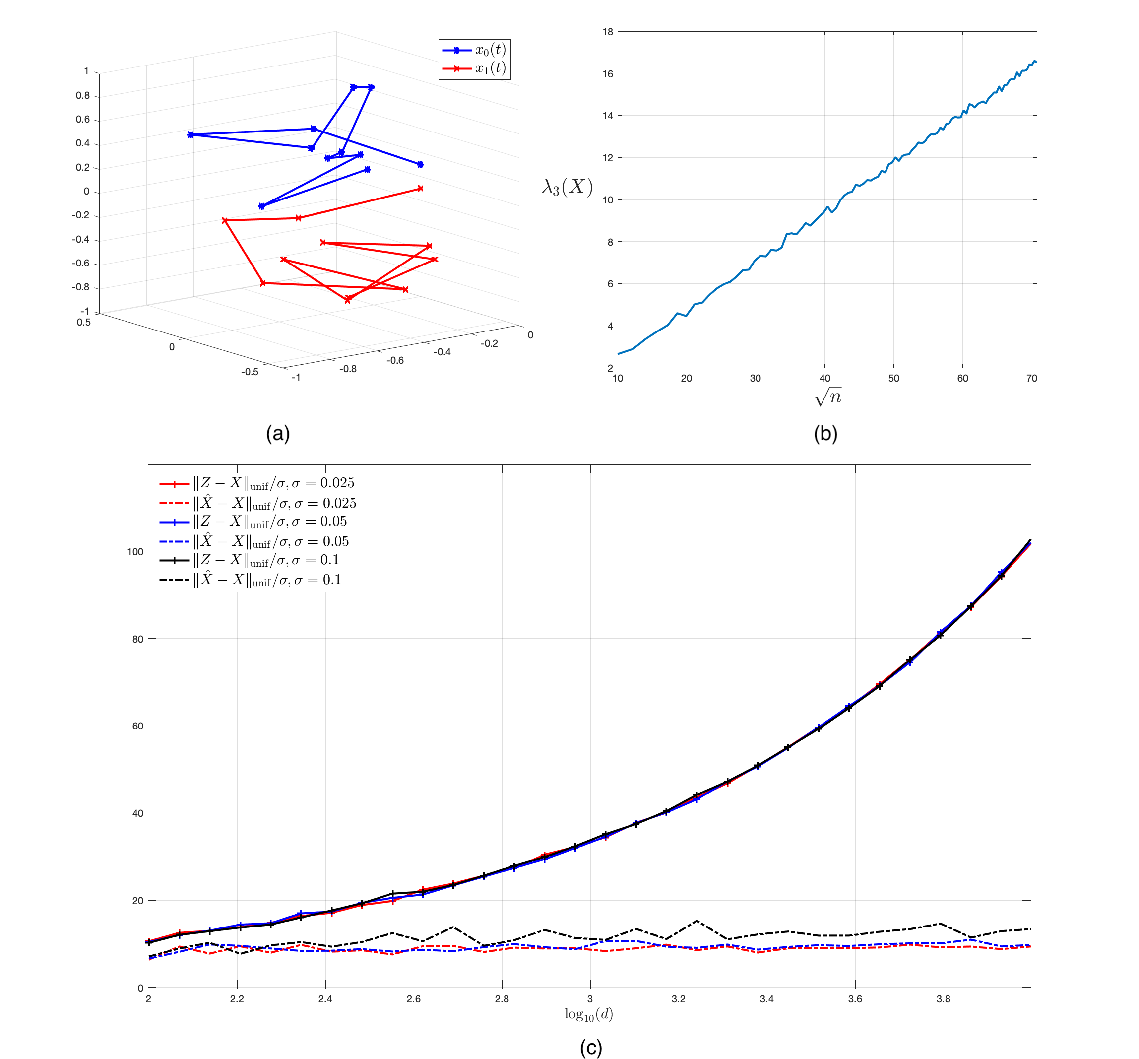
Figure 1: Properties of data generated from two zig-zag lines. (a) The two zigzag lines where the clean data is generated from. They are separated by parallel hyperplanes with a distance of $0.2$. (b) The third singular value of the clean data $X\in\mathbb{R}^{n\times 3}$, which scales linearly with the square root of the sample size $n$. (c) The normalized uniform errors of the noisy data $Z$, denoised data $\hat{X}$ achieved at different dimension $d.$ With a fixed standard deviation of the noise $\sigma$, the uniform errors obtained from the noisy data $Z\in\mathbb{R}^{n\times d}$ increase with the dimension $d$ and sample size $n=0.1d$. However, the uniform errors obtained from the denoised data $\hat{X}$ remain approximately constant. The results are consistent with different standard deviations, $\sigma=0.025,0.05,$ and $0.1$.

To support our theoretical results, we provide some numerical examples in this section. We consider a two-class clustering setting where the clean data are sampled from two separated low-dimensional zigzag lines that are embedded in a high-dimensional space. In detail, we first generate two zigzag lines, each consisting of 10 segments within a unit ball in $\mathbb{R}^{3}$, as seen in Figure 1(a). Then we embedded them into $d$-dimensional space by an orthonormal matrix $\Omega\in\mathbb{R}^{d\times 3}$ with $d$ being some large number to be specified later. Denote the embedded zigzag lines as $x_{0}(t)$ and $x_{1}(t)$ for $0\leq t\leq 1$. The clean data are generated as $X_{i}=\Omega\,x_{\ell(i)}(t_{i})$, where $\ell(i)\sim Bernoulli(1/2)$ and $t_{i}\sim U[0,1]$, $i\in[n]$. Here $\ell(i)$ can be regarded as the label of this sample and our goal is to recover it. Finally, we add the noise to the clean data, where $Z_{i}=X_{i}+\xi_{i}$, $\xi_{i}\sim\mathcal{N}(0,\sigma^{2}I_{d})$. The algorithm will be applied to the noisy data $Z$.

We first check the uniform error of PCA-denoised data by Algorithm 1. The error in Theorem 1 requires the information of $\lambda_{r}(X)$, which is shown to be $O(\sqrt{n})$ in Proposition 2 for the zigzag scenario. According to the generation procedure, the clean data $X$ lies in the space with a dimension of $r=3$, so we calculate $\lambda_{3}(X)$ for $n$ ranging from $10^{2}$ to $70^{2}$. The embedding $\Omega$ does not change the eigenvalue, and $\lambda_{3}(X)=\lambda_{3}(x)$ where $x=(x_{\ell(1)}(t_{1}),\cdots,x_{\ell(n)}(t_{n}))$. We calculate it based on $x$ so the dimension $d$ does not affect the result. As seen in Figure 1(b), $\lambda_{3}(X)$ scales linearly with $\sqrt{n}$, which follows Proposition 2. Such a result indicates the simplified uniform error in Theorem 1 holds, that $\|X-\hat{X}\|_{\text{unif}}=O(\sigma+\sigma^{4}\log n)$ when $d=c_{d}n$. We fix $n=0.1d$ and let $d$ range from $10^{2}$ to $10^{4}$, where the added noise $\sigma\in\{0.0025,0.05,0.1\}$. Figure 1(c) presents the uniform error of the noisy data $Z$ and the denoised data $\hat{X}$ by Algorithm 1. It can be found that $\|\hat{X}-X\|_{\text{unif}}/\sigma$ stays constant throughout the regime while $\|Z-X\|_{\text{unif}}/\sigma$ grows as $\sqrt{d}$. Even in the high-dimensional case that $d=10n$, the PCA-denoising algorithm can reduce the curse of dimension and reduce the uniform error to be $O(\sigma)$.

We then investigate the denoising effects on downstream statistical inference, particularly in the graphical Laplacian eigenvectors and spectral clustering. Let $L(B)$ denote the graph Laplacian of any data matrix $B$. We find the eigenvector corresponding to the second smallest eigenvalue, which is called the Fielder eigenvector. Denote it as $\eta_{2}(B)$. It is well known that the component signs of $\eta_{2}(B)$ can be used to infer cluster labels (Von Luxburg et al. (2008)). We are interested in the error of the Fiedler eigenvectors from different data sources and the associated clustering results.

To illustrate the importance of the uniform error, we consider three data matrices in this study: the clean data $X$, the denoised data with small uniform error $\hat{X}$, and a new data set $\tilde{X}$ with errors not uniformly distributed. To make the comparison fair, the new matrix $\tilde{X}$ has the same average error as $\hat{X}$, i.e.

$$\frac{1}{n}\sum_{i=1}^{n}\|X_{i}-\hat{X}_{i}\|^{2}=\frac{1}{n}\sum_{i=1}^{n}\|X_{i}-\tilde{X}_{i}\|^{2}.$$ (28)

We design $\tilde{X}$ in the way that some samples have a large error and other samples have no errors. In detail, we randomly select 10% of indices as $\mathcal{I}$, and define $\tilde{X}_{i}$ as:

$$\tilde{X}_{i}=\begin{cases}X_{i},\quad&\text{if }i\in\mathcal{I}^{c};\\ \alpha X_{i}+(1-\alpha)Z_{i},\quad&\text{if }i\in\mathcal{I};\end{cases}$$

where $\alpha\in(0,1)$ is a constant that ensures (28). In other words, 90% of data in $\tilde{X}$ are clean; the others have $i.i.d.$ error as $(1-\alpha)\xi_{i}$, where $\alpha$ is chosen so that the average error is the same with $\hat{X}$. Comparisons between $\eta_{2}(\hat{X})$ and $\eta_{2}(\tilde{X})$ explain how uniform error is important in practice.

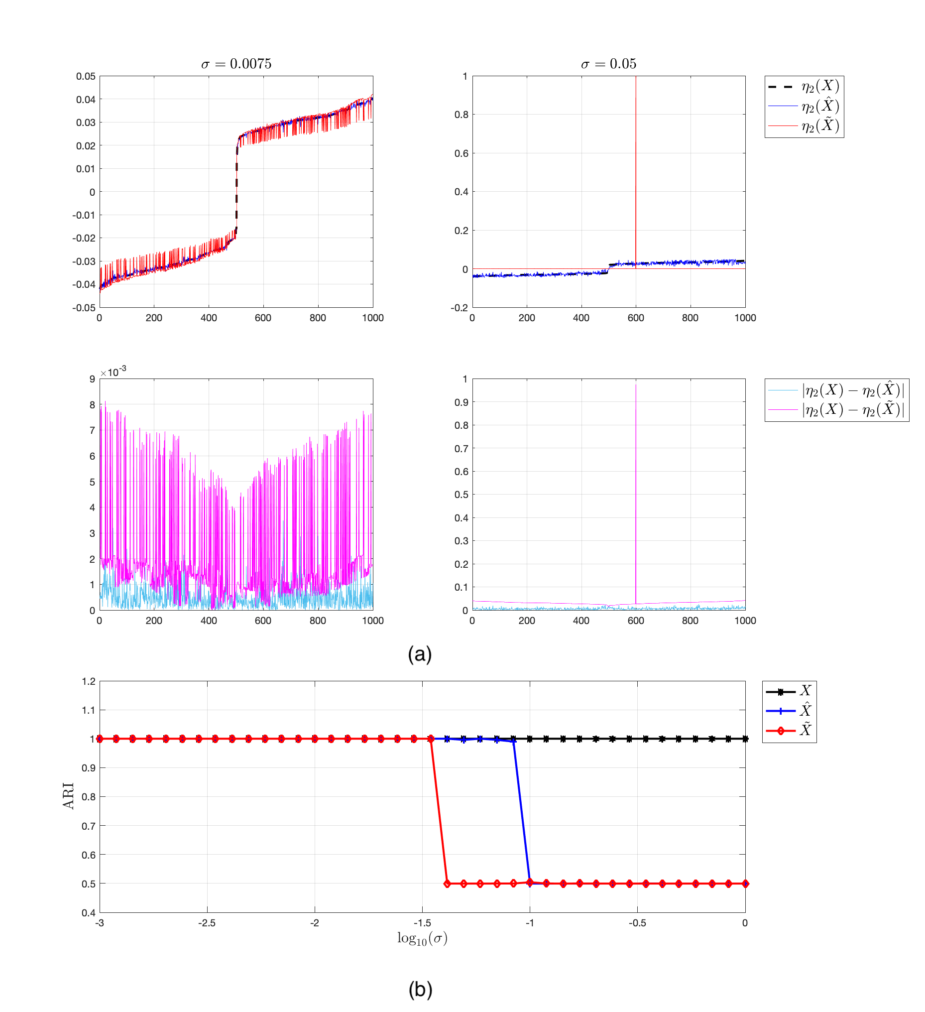
Figure 2: Spectral clustering with different data sources. (a) The comparisons among the Fielder eigenvectors of the Laplacian formed by the clean data denoted as $\eta_{2}(X)$, the averaged denoised data denoted as $\eta_{2}(\tilde{X})$ and the denoised data $\eta_{2}(\hat{X}),$ at two different noise levels. The first row plots the second (Fiedler) eigen-vectors of the graph Laplacian obtained by the clean data $X$, the denosied data $\hat{X}$ and “averaged denoised” data $\tilde{X}$. They are denoted by $\eta_{2}(X),\eta_{2}(\hat{X})$ and $\eta_{2}(\tilde{X})$ respectively. The second row plots the pointwise absolute difference betweens $(\eta_{2}(X),\eta_{2}(\hat{X}))$ and $(\eta_{2}(X),\eta_{2}(\tilde{X}))$. We choose the standard deviation of the noise to be $\sigma=0.0075$ and $0.05$, corresponding to the two columns. (b) The comparisons between the adjusted rand indices (ARI) achieved by spectral clustering using clean data $X$, denoised data $\hat{X}$ and the “averaged denoised” data $\tilde{X}$ under different scale of noise $\sigma.$

We fix $d=5000$ and $n=1000$. The bandwidth for graphical Laplacian is chosen as $b=\sqrt{0.005}$. We first compare the Fiedler eigenvectors from three data matrices $X$, $\hat{X}$ and $\tilde{X}$ at two noise levels $\sigma=0.0075$ and $\sigma=0.05$, shown in Figure 2(a). We adjust the order of data samples so that samples from $x_{0}(t)$ comes first and those from $x_{1}(t)$ are all at last. In the top panel of Figure 2(a), we can see the sign $\eta_{2}(X)$ meets the label $\ell$. For the two data with small noise $\sigma=0.0075$, $\eta_{2}(\hat{X})$ and $\eta_{2}(\tilde{X})$ are close to $\eta_{2}(X)$ at a large scale. The error of $\eta_{2}(\hat{X})$ is uniformly small but $\eta_{2}(\tilde{X})$ has spiked errors. This is consistent with Proposition 5. When $\sigma$ increases from $0.0075$ to $0.05$, the spiked error in $\|\tilde{X}_{i}-X_{i}\|$ is so large that the distance-based clustering algorithm fails. Meanwhile, the Fiedler eigenvector obtained by $\hat{X}$ can still preserve the correct cluster labels. We then study the clustering results of the three data matrices for $\sigma$ ranging from $10^{-3}$ to $1$, shown in Figure 2(b). We use the adjusted rand index (ARI) to measure the clustering accuracy, where $ARI=1$ indicates a perfect clustering and $ARI=0.5$ means a random guess. The performance of clustering using other data sources would of course depend on the strength of noise. Not surprisingly, because of the crash in estimating $\eta_{2}(X)$, using $\tilde{X}$ fails when $\sigma\geq 0.05$ and using $\hat{X}$ gives a satisfactory clustering result till $\sigma\geq 0.1$.

References

• Abbe and Sandon [2015] Emmanuel Abbe and Colin Sandon. Community detection in general stochastic block models: Fundamental limits and efficient algorithms for recovery. In 2015 IEEE 56th Annual Symposium on Foundations of Computer Science, pages 670–688. IEEE, 2015.
• Abbe et al. [2020] Emmanuel Abbe, Jianqing Fan, Kaizheng Wang, and Yiqiao Zhong. Entrywise eigenvector analysis of random matrices with low expected rank. Annals of statistics, 48(3):1452, 2020.
• Abdi and Williams [2010] Hervé Abdi and Lynne J Williams. Principal component analysis. Wiley interdisciplinary reviews: computational statistics, 2(4):433–459, 2010.
• Bao et al. [2021] Zhigang Bao, Xiucai Ding, and Ke Wang. Singular vector and singular subspace distribution for the matrix denoising model. The Annals of Statistics, 49(1):370–392, 2021.
• Brunton and Kutz [2022] Steven L Brunton and J Nathan Kutz. Data-driven science and engineering: Machine learning, dynamical systems, and control. Cambridge University Press, 2022.
• Bubeck and Luxburg [2009] Sébastien Bubeck and Ulrike von Luxburg. Nearest neighbor clustering: A baseline method for consistent clustering with arbitrary objective functions. The Journal of Machine Learning Research, 10:657–698, 2009.
• Cai and Zhang [2018] T Tony Cai and Anru Zhang. Rate-optimal perturbation bounds for singular subspaces with applications to high-dimensional statistics. Annals of Statistics, 46(1):60–89, 2018.
• Cape et al. [2019a] Joshua Cape, Minh Tang, and Carey E Priebe. The two-to-infinity norm and singular subspace geometry with applications to high dimensional statistics. The Annals of Statistics, 47(5):2405–2439, 2019a.
• Cape et al. [2019b] Joshua Cape, Minh Tang, and Carey E Priebe. Signal-plus-noise matrix models: eigenvector deviations and fluctuations. Biometrika, 106(1):243–250, 2019b.
• Chen et al. [2022] Xi Chen, Qiang Liu, and Xin T Tong. Dimension independent excess risk by stochastic gradient descent. Electronic Journal of Statistics, 16(2):4547–4603, 2022.
• Chen et al. [2021] Yuxin Chen, Yuejie Chi, Jianqing Fan, Cong Ma, et al. Spectral methods for data science: A statistical perspective. Foundations and Trends® in Machine Learning, 14(5):566–806, 2021.
• Cressie and Wikle [2015] Noel Cressie and Christopher K Wikle. Statistics for spatio-temporal data. John Wiley & Sons, 2015.
• Davis and Kahan [1970] Chandler Davis and William Morton Kahan. The rotation of eigenvectors by a perturbation. iii. SIAM Journal on Numerical Analysis, 7(1):1–46, 1970.
• Ding [2020] Xiucai Ding. High dimensional deformed rectangular matrices with applications in matrix denoising. Bernoulli, 26(1):387 – 41, 2020.
• Dong and Tong [2021] Jing Dong and Xin T Tong. Replica exchange for non-convex optimization. The Journal of Machine Learning Research, 22(1):7826–7884, 2021.
• Donoho and Gavish [2014] David Donoho and Matan Gavish. Minimax risk of matrix denoising by singular value thresholding. The Annals of Statistics, 42(6):2413–2440, 2014.
• Donoho et al. [2000] David L Donoho et al. High-dimensional data analysis: The curses and blessings of dimensionality. AMS math challenges lecture, 1(2000):32, 2000.
• Fan et al. [2018] Jianqing Fan, Weichen Wang, and Yiqiao Zhong. An $l_{\infty}$ eigenvector perturbation bound and its application to robust covariance estimation. Journal of Machine Learning Research, 18(207):1–42, 2018.
• Hartigan and Wong [1979] John A Hartigan and Manchek A Wong. Algorithm as 136: A k-means clustering algorithm. Journal of the royal statistical society. series c (applied statistics), 28(1):100–108, 1979.
• Hastie et al. [2009] Trevor Hastie, Robert Tibshirani, Jerome H Friedman, and Jerome H Friedman. The elements of statistical learning: data mining, inference, and prediction, volume 2. Springer, 2009.
• Jin and Wang [2016] Jiashun Jin and Wanjie Wang. Influential features pca for high dimensional clustering. The Annals of Statistics, 44(6):2323–2359, 2016.
• Jin et al. [2017] Jiashun Jin, Zheng Tracy Ke, and Wanjie Wang. Phase transitions for high dimensional clustering and related problems. The Annals of Statistics, 45(5):2151–2189, 2017.
• Johnstone and Lu [2009] Iain M Johnstone and Arthur Yu Lu. On consistency and sparsity for principal components analysis in high dimensions. Journal of the American Statistical Association, 104(486):682–693, 2009.
• Jolliffe [2005] Ian Jolliffe. Principal component analysis. Encyclopedia of statistics in behavioral science, 2005.
• Jolliffe [1972] Ian T Jolliffe. Discarding variables in a principal component analysis. i: Artificial data. Journal of the Royal Statistical Society Series C: Applied Statistics, 21(2):160–173, 1972.
• Laurent and Massart [2000] Beatrice Laurent and Pascal Massart. Adaptive estimation of a quadratic functional by model selection. Annals of Statistics, pages 1302–1338, 2000.
• Leeb [2021] William E Leeb. Matrix denoising for weighted loss functions and heterogeneous signals. SIAM Journal on Mathematics of Data Science, 3(3):987–1012, 2021.
• Mei et al. [2018] Song Mei, Yu Bai, and Andrea Montanari. The landscape of empirical risk for nonconvex losses. The Annals of Statistics, 46(6A):2747–2774, 2018.
• Menard [2002] Scott Menard. Applied logistic regression analysis. Number 106. Sage, 2002.
• Montanari et al. [2018] Andrea Montanari, Feng Ruan, and Jun Yan. Adapting to unknown noise distribution in matrix denoising. arXiv preprint arXiv:1810.02954, 2018.
• Nadakuditi [2014] Raj Rao Nadakuditi. Optshrink: An algorithm for improved low-rank signal matrix denoising by optimal, data-driven singular value shrinkage. IEEE Transactions on Information Theory, 60(5):3002–3018, 2014.
• Omran et al. [2007] Mahamed GH Omran, Andries P Engelbrecht, and Ayed Salman. An overview of clustering methods. Intelligent Data Analysis, 11(6):583–605, 2007.
• Pollard [1981] David Pollard. Strong consistency of k-means clustering. The Annals of Statistics, pages 135–140, 1981.
• Rakhlin and Caponnetto [2006] Alexander Rakhlin and Andrea Caponnetto. Stability of $k$-means clustering. Advances in neural information processing systems, 19, 2006.
• Rao [1964] C Radhakrishna Rao. The use and interpretation of principal component analysis in applied research. Sankhyā: The Indian Journal of Statistics, Series A, pages 329–358, 1964.
• Reiss and Wahl [2020] Markus Reiss and Martin Wahl. Nonasymptotic upper bounds for the reconstruction error of pca. The Annals of Statistics, 48(2):1098–1123, 2020.
• Seber and Lee [2003] George AF Seber and Alan J Lee. Linear regression analysis, volume 330. John Wiley & Sons, 2003.
• Shalev-Shwartz and Ben-David [2014] Shai Shalev-Shwartz and Shai Ben-David. Understanding machine learning: From theory to algorithms. Cambridge university press, 2014.
• Shepard [1962] Roger N Shepard. The analysis of proximities: multidimensional scaling with an unknown distance function. i. Psychometrika, 27(2):125–140, 1962.
• Singer [2006] Amit Singer. From graph to manifold laplacian: The convergence rate. Applied and Computational Harmonic Analysis, 21(1):128–134, 2006.
• Singh and Harrison [1985] Ashbindu Singh and Andrew Harrison. Standardized principal components. International journal of remote sensing, 6(6):883–896, 1985.
• Tukey [1960] John W Tukey. A survey of sampling from contaminated distributions. contributions to probability and statistics. Essays in honor of harold hotelling, 1960.
• Vershynin [2010] Roman Vershynin. Introduction to the non-asymptotic analysis of random matrices. arXiv preprint arXiv:1011.3027, 2010.
• Von Luxburg [2007] Ulrike Von Luxburg. A tutorial on spectral clustering. Statistics and computing, 17:395–416, 2007.
• Von Luxburg et al. [2008] Ulrike Von Luxburg, Mikhail Belkin, and Olivier Bousquet. Consistency of spectral clustering. The Annals of Statistics, pages 555–586, 2008.
• Wahba et al. [1999] Grace Wahba et al. Support vector machines, reproducing kernel hilbert spaces and the randomized gacv. Advances in Kernel Methods-Support Vector Learning, 6:69–87, 1999.
• Wedin [1972] Per-Åke Wedin. Perturbation bounds in connection with singular value decomposition. BIT Numerical Mathematics, 12:99–111, 1972.
• Yu et al. [2015] Yi Yu, Tengyao Wang, and Richard J Samworth. A useful variant of the davis–kahan theorem for statisticians. Biometrika, 102(2):315–323, 2015.
• Zhang et al. [2022] Anru R Zhang, T Tony Cai, and Yihong Wu. Heteroskedastic pca: Algorithm, optimality, and applications. The Annals of Statistics, 50(1):53–80, 2022.