Counting occurrences of patterns in permutations

Abstract

We develop a new, powerful method for counting elements in a multiset. As a first application, we use this algorithm to study the number of occurrences of patterns in a permutation. For patterns of length 3 there are two Wilf classes, and the general behaviour of these is reasonably well-known. We slightly extend some of the known results in that case, and exhaustively study the case of patterns of length 4, about which there is little previous knowledge. For such patterns, there are seven Wilf classes, and based on extensive enumerations and careful series analysis, we have conjectured the asymptotic behaviour for all classes.

Finally, we investigate a proposal of Blitvić and Steingrímsson as to the range of a parameter for which a particular generating function formed from the occurrence sequences is itself a Stieltjes moment sequence.

1 Introduction

Let $\pi$ be a permutation on $[n]$ and $\tau$ be a permutation on $[k].$ $\tau$ is said to occur as a pattern in $\pi$ if for some sub-sequence of $\pi$ of length $k$ all the elements of the sub-sequence occur in the same relative order as do the elements of $\pi.$ If the permutation $\tau$ does not occur in $\pi,$ then this is said to be a pattern-avoiding permutation or PAP.

If the permutation $\tau$ occurs $r$ times, it is said to be an $r$-occurrence of the pattern. Clearly, pattern-avoidance corresponds to the case $r=0.$

Let $s_{n}(\tau)$ denote the number of permutations of $[n]$ that avoid the pattern $\tau.$ Stanley and Wilf conjectured, and Marcus and Tardos [35] subsequently proved, that for any pattern $\tau$ in $[k]$ the limit $\lim_{n\to\infty}s_{n}(\tau)^{\frac{1}{n}}=\lambda$ exists and is finite. This means that the number of PAPs grows exponentially with $n,$ whereas of course the number of permutations of $n$ grows factorially.

For the more general problem of $r$-occurrences of a given pattern $\tau,$ a similar result holds, and the exponential growth rate $\lambda$ is independent of $r,$ proved by Mansour, Rastegar and Roitershtein [33].

There are 6 possible permutations of length three, and the number of permutations of length $n$ avoiding any of these 6 patterns is given precisely by $C_{n}=\frac{1}{n+1}\binom{2n}{n}\sim\frac{4^{n}}{\sqrt{\pi n^{3}}},$ where $C_{n}$ denotes the $n^{th}$ Catalan number. That is to say, all 6 possible patterns have the same exponential growth-rate as PAPs. Alternatively expressed, there is only one Wilf class for length-3 PAPs.

For length-4 PAPs there are three Wilf classes. Typical representatives of the three classes are $1234,$ $1342$ and $1324.$ The generating function for the first two classes is known.

In the first case, first proved by Gessel [15], the generating function is D-finite, satisfying a third-order linear, homogeneous ODE and $s_{n}(1234)\sim\frac{81\sqrt{3}\cdot 9^{n}}{16\pi\cdot n^{4}}.$

In the second case, first proved by Bóna [1], the generating function is algebraic, and $s_{n}(1342)\sim\frac{64\cdot 8^{n}}{243\sqrt{\pi}\cdot n^{5/2}}.$

The third case has not been solved, but extensive numerical work by Conway et al. [9] suggests that $s_{n}(1324)\sim C\cdot\mu^{n}\cdot\mu_{1}^{\sqrt{n}}\cdot n^{g},$ where $\mu\approx 11.598$ (and possibly $9+3\sqrt{3}/2$ exactly), $\mu_{1}\approx 0.0400,$ and $g\approx-1.1.$ The appearance of the sub-dominant term $\mu_{1}^{\sqrt{n}}$ is referred to as a stretched exponential term. If present, that would suffice to prove that the generating function is not D-finite [14].

Thus these three Wilf classes have generating functions that are D-finite, algebraic, and (almost certainly) non-D-finite respectively.

In this article we study the more general question of the behaviour of the generating function of $r$-occurrences of a given pattern in a permutation of length $n.$ The problem of pattern-avoiding permutations thus corresponds to the case $r=0.$

For this more general problem, it is known that, for patterns of length-3, there are two Wilf classes, one corresponding to the two patterns $123$ and $321,$ and the other corresponding to the remaining four permutations of length 3.

Surprisingly, the $r$-dependence of the two classes is quite different. Let $\psi_{r}(n)$ denote the number of permutations of length $n$ containing exactly $r$ occurrences of the nominated pattern. Then for the class 123 and 321 one has

$$\psi_{r}(n)=\frac{Q_{2r}(n)(2n-r)!}{(n+2r+1)!(n-r)!}\sim\frac{C_{r}\cdot 4^{n}}{n\sqrt{n\pi}}$$ (1)

where $Q_{2r}(n)$ is a polynomial with integer coefficients of degree $2r.$ For small values of $r,$ the amplitude coefficient $C_{r}$ appears to increase exponentially, growing seemingly like $\lambda^{r},$ where the growth constant $\lambda\approx 2.67.$ That is to say, the asymptotics remain unchanged, and only the amplitude, or premultiplying constant changing with $r.$ However this exponential increase in the amplitude cannot continue indefinitely, and indeed must decline toward zero as $r$ becomes large, as we explain below.

For the second class, corresponding to patterns 132, 231, 213, 312, Mansour and Vainshtein [34] show that

$$\psi_{r}(n)=\frac{Q_{r}(n)(2n-3r)!}{n!r!(n-r-2)!}\sim\frac{4^{n-3r/2}\cdot n^{r-3/2}}{r!\sqrt{\pi}}$$ (2)

where $Q_{r}(n)$ is a polynomial of degree $3(r-1),$ whose leading-order term is precisely $n^{3(r-1)}.$ Here the asymptotics are quite different. The amplitude changes in a very regular way, but the subdominant power-law exponent increases by 1 as $r$ increases by 1.

Another noteworthy property of these $r$-occurrences is that, while the counting sequences $\psi_{r}(n)$ are known or conjectured to be Stieltjes moment sequences for the case $r=0,$ as discussed in Bostan et al. [7], this is not the case for $r>0,$ for all the cases we have studied. We discuss this further below.

Aspects of this problem have been previously studied by several authors. For the class 132, Noonan and Zeilberger [41] conjectured the result for $r=1,$ subsequently proved by Bóna [3]. Bóna also proved [1] that the number of $r$-occurrences of the pattern 132 is P-recursive in the size. Equivalently, the ordinary generating function is D-finite. He then proved the stronger statement that the generating function is algebraic.

Mansour and Vainshtein [34] proved the corresponding result for $r=2$ and then gave conjectural results for $r\leq 6,$ and conjectured the structure of the general formula.

For the increasing subsequence 123, Noonan [40] proved the result for $r=1,$ and Noonan and Zeilberger [41] conjectured the result for $r=2.$ This was subsequently proved by Fulmek [12], who also gave conjectured results for $r=3$ and $r=4.$ These were subsequently proved by Callan [8]. Nakamura and Zeilberger [39] developed a Maple package implementing a functional equation that readily generated terms for the cases $r\leq 7,$ and gave the corresponding expressions for $\psi_{r}(n)$ for $r\leq 7.$

In [4] Bóna proved that, for the monotone pattern $1234\cdots k,$ the distribution function of $r$-occurrences is asymptotically normal. Indeed, this is true for any classical pattern, a result first claimed to be proved by Bóna in [5]. It was unequivocally proved by Janson et al. in [28], and can also be proved, perhaps even more easily, by the methods developed by Hofer in [22].

As far as we are aware, the general situation for patterns of length 4 has not previously been studied, due in large part to the difficulty of generating coefficients of the underlying generating functions, though as we note below, there have been some series generated. We have developed an algorithm for this purpose, and find that of the $4!=24$ permutations of length-4, there are now seven effective Wilf classes. They are as follows:

$$I: 1234,4321$$

$$II: 1243,2134,3421,4312,$$

$$III: 1432,2341,3214,4123$$

$$IV: 2143,3412,$$

$$V: 1324,4231$$

$$VI: 1342,1423,2314,2431,3124,3241,4132,4213$$

$$VII: 2413,3142$$

By effective Wilf class in this context we mean that the number of $r$-occurrences of any pattern in the class in a permutation of length $n$ is the same, irrespective of the value of $r.$ For pattern-avoiding permutations, the first four classes above correspond to a single Wilf class, so these will all have coefficient growth $9^{n}.$ The fifth entry, with coefficient growth $\mu^{n},$ where $\mu\approx 11.598$ [9] corresponds to another Wilf class, and the third Wilf class for PAPs comprises the patterns in class VI and VII above, with coefficient growth $8^{n}.$

It is worth remarking that, for contiguous PAPs, there are also 7 Wilf classes, and 5 of those 7 are the same as those given above. However the two problems differ in classes III and VI. As far as we can see, there is no reason that these two problems should be connected, so it’s not surprising that there is a difference between the class distributions. It is perhaps surprising that 5 classes are the same.

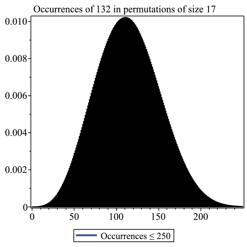
Figure 1: Histogram of normalised 132 occurrences.

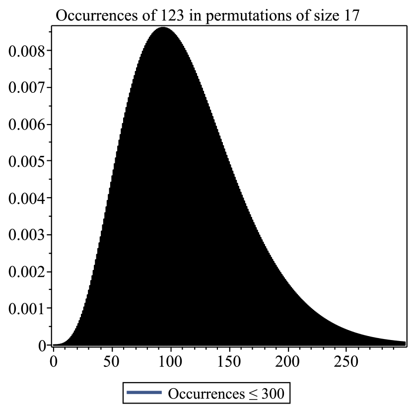
Figure 2: Histogram of normalised 123 occurrences.

2 Generating the number of occurrences of a given pattern

In [37] Minato came up with an innovative and general algorithm for counting pattern avoiding permutations. It involved a straightforward algorithm operating upon sets of permutations that generates all permutations containing the pattern, and then, crucially, an efficient computational representation of said sets taking up space and time much smaller than the number of elements in the set. This makes the algorithm much more efficient in practice than other known general algorithms that examine each pattern avoiding permutation individually. In [23], Inoue improved the set representation to make the algorithm even more efficient in practice.

We use the same algorithm operating upon sets, except apply it to multisets instead of sets. That is, each element in the set has a multiplicity. The union of two multisets in our context sums the multiplicities of each element. A consequence of the construction algorithm is that the resulting set contains each permutation containing the pattern, with a multiplicity equal to the number of occurrences of the given pattern. It is then an efficient operation on the multiset to obtain the number of elements with each multiplicity. This is the desired enumeration.

We generalize the back end set representation in [23] to handle multisets. This actually is a potentially generally useful multiset representation for combinatorics. In practice, it ends up being reasonably efficient. As a more complex structure containing more information than the simple set it takes somewhat more time and memory than the simple set, but is still vastly more efficient than techniques that consider elements individually.

The rest of this section goes into more detail, firstly on the set construction algorithm, secondly on the method of representing a set of permutations as a binary decision tree, and thirdly on generalizing binary decision trees to contain multiplicities to be able to represent multisets.

2.1 Set construction algorithm

Here we summarise the algorithm used in [37] and [23], leaving out many of the details and concentrating upon the set operations used.

For the following discussion, $n$ unless otherwise specified is the number of elements in the desired permutation, and $k\leq n$ is the length of the pattern.

There is a three step process to generate the set of all pattern containing permutations.

Step 1 generates all permutations $A$ whose first $k$ elements are in increasing order. There are $\binom{n}{k}$ ways of choosing the first $k$ elements, and $(n-k)!$ ways of arranging the remaining elements, for a total of $n!/k!$ elements in this set. We will not repeat the details of the construction here, but mention that it generates each element exactly once and requires $O(n^{2})$ set unions and set compositions with a “unit” permutation (a swap of two elements in [37] and a rotation in [23]). If operating on a multiset, each element is created with multiplicity $1$.

As an example, if $n=4$ and $k=2$ for the pattern $21$ (only the length matters for this step), $A=\{1234,1243,1324,1342,1423,1432,2314,2341,2413,2431,3412,3421\}$ are the elements whose first $k=2$ elements are in order.

Step 2 makes a new set $B\times A$ that just rearranges the first $k$ elements of the above set $A$ to match the pattern. That is, $B$ is a set containing a single element which is a permutation consisting of the pattern followed by the remaining $n-k$ elements of the identity permutation.

As an example, if $n=4$ and $k=2$ for the pattern $21$, $B=\{2134\}$.

The required set operation $\times$ is a cross product, taking two sets (or multisets) $A$ and $B$ and producing a set $\{a\times b:a\in A,b\in B\}$ where $a\times b$ is the composition of the permutations $a$ and $b$. If multisets are being used, then the cardinality (sum of the multiplicities of each element) of $A\times B$ is the product of the cardinalities of $A$ and $B$.

In the running example, the only difference is that the first two elements are exchanged to match the pattern $21$. Giving the elements in the same order as for $A$, $B\times A=\{2134,2143,3124,3142,4123,4132,3214,3241,4213,4231,4312,4321\}$.

$B$ has cardinality 1. The cardinality of $B\times A$ is the same as $A$: that is, $n!/k!$ elements each with multiplicity $1$.

Step 3 distributes the $k$ first elements of each permutation in $B\times A$ over the $\binom{n}{k}$ possible positions in the permutation. This is done by constructing a set $C$ of permutations that take the first $k$ elements to each of the $\binom{n}{k}$ possible positions in the permutation. This construction is similar to the construction of $A$, requiring set unions, and composition with unit permutations. The cardinality of $C$ is $\binom{n}{k}$ elements each with multiplicity 1.

The set of pattern containing permutations is then $C\times B\times A$. The same pattern may occur multiple times of course.

For $n=4$ and $k=2$, $C=\{1234,1324,1342,3124,3142,3412\}$. Unfortunately $C\times B\times A$ is too many elements to helpfully list, but as a few examples, the first permutation in $C$ is the identity which when crossed with $B\times A$ changes nothing. The second element in $C$, $1324$ (pattern positions $1$ and $3$), when operating on $2134$ (pattern values $2$ and $1$) produces $2314$. Of course there is another instance of that pattern in $C\times B\times A$: $3124$ (pattern positions $2$ and $3$) operating on $3124$ (pattern values $3$ and $1$) also produces $2314$.

As a multiset, the number of ways the same pattern occurs in this construction for a permutation $p\in C\times B\times A$ (the multiplicity of $p$) is the number of occurrences of the pattern in $p$. This is exactly what is desired.

2.2 Set representation

As mentioned before, the obvious simple computational set representation explicitly listing all elements would result in dreadful performance, as there are close to $n!$ elements in $C\times B\times A$.

The big inspiration of [37] was to use binary decision diagrams (BDDs) to represent these sets. A BDD represents a Boolean function of $N$ Boolean variables. A Boolean function $f(v_{0},...,v_{N-1})$ can be considered to represent a set $F$ with an element $(v_{0},...,v_{N-1})$ in $F$ iff $f(v_{0},...,v_{N-1})$ is true. For many combinatorial problems BDDs produce a very compact representation of these sets [31].

A BDD consists of a list of $N$ Boolean variables ${v_{0},...v_{N-1}}$, a table consisting of some number of rows, and a starting index pointing to one of these rows. Each row consists of three elements - a variable index, and two row indices (LO and HI). There are two special row indices meaning true (often called 1 or $\top$) or false (often called 0 or $\bot$). One can store multiple values in the table, in which case each starting index is effectively a function. To evaluate a function implied by a row index, first check to see if it is one of the two special true or false references. If so, we are done. Otherwise read the row corresponding to that index. Check the variable that row references. If the variable is false, take the first row index (LO) in the current row. Otherwise take the second row index (HI). Replace the original row index with this new index, and repeat the above operation recursively. See figure 3 for an example.

In order to promote uniqueness, the following rules are required:

• If row $i$ contains a reference to a non-terminal row $j$, then the variable index in row $i$ must come before the variable index in row $j$.

• No two rows in the table should be identical (if one were tempted to add a new row the same as an existing row, just use the existing row).

• Each row should matter. No row should have the same indices regardless of the variable state (except possibly the special case of the two terminal rows, if they are explicitly stored).

This produces uniqueness (up to row renumbering) for any given function, and, possibly unintuitively, produces a compact representation for many combinatorics problems.

(a) Graphical representation. One starts from the top of the diagram. A circle represents a decision point. The number $i$ in the circle is the variable index. Take the LO choice (dashed) if $v_{i}$ is false and the HI choice (solid) if $v_{i}$ is true. A square is a terminal : $\top$ means true and $\bot$ means false.

$v_{0}$	$v_{1}$	output
false	false	true
false	true	true
true	false	false
true	true	true

(b) Truth table. This shows the result of the BDD for all possible combinations of values of $v_{0}$ and $v_{1}$

row	variable	LO	HI
3	0	1	2
2	1	0	1
1	special true $\top$
0	special false $\bot$

Start from row 3.

(c) BDD table. This is the computer representation of the BDD. Each row has an index (the row column). For each row one stores a variable index, and the LO and HI indices to other columns in this table.

Figure 3: Three different representations of a BDD of two variables.

An example BDD using notation similar to [31] is given in figure 3

ZDDs are very similar to BDDs, except instead of suppressing rows whose two children are identical, one suppresses rows where a true value of the variable would lead to the false special row index. This ends up being more compact than a BDD when most variables are false in most solutions.

The detailed mechanics of implementation of a BDD or ZDD are well described in [31].

Of course, we need a set of permutations, not a set of choices of a set of binary variables. In [37], Minato defined a set of basis permutations - the $N=n(n-1)/2$ pairwise swaps of each element of the $n$ elements of the permutation. Minato also defined a canonical order. Each permutation then has a unique set of these $n(n-1)/2$ basis permutations that combine to produce it. A $\pi$DD is a zero suppressed binary decision diagram using this encoding to represent a set of permutations.

The encoding is improved in [23] so as to have a basis of $n(n-1)/2$ rotations of the elements between each choice of two elements of the permutation. This variant of a $\pi$DD is called a Rot-$\pi$DD. This basis set produces a much smaller representation of the set $A$ than a $\pi$DD which intuitively and empirically leads to a smaller representation of $C\times B\times A$, and a more efficient algorithm.

The required set operations are set union, unit and empty set creation, the cross product, and set cardinality.

Unit and empty set creation are trivial and will clearly not create an invalid permutation element given a valid input. The set union and cardinality operations are identical to the standard BDD or ZDD operations [31], and will not create new (and therefore possibly invalid) permutation elements.

The cross product is not a standard BDD operation as it needs to take into account the composition of permutations and the requirement for a canonical representation of each permutation. In practice this is comparable to the standard BDD or ZDD cross product, but is a little more fiddly. Details are described in [37] and [23].

There is another operation used in practice to create the sets $A$ and $C$ which is really a special case of the set cross product, where one of the sets is a single element set containing a permutation which is one of the basis permutations. For efficiency this is implemented as a special case. Details are described in [37] and [23].

There are no useful theoretical bounds on the performance of $\pi$DDs or Rot-$\pi$DDs for use in the above algorithm to enumerate pattern avoiding permutations, but empirically they are vastly superior to algorithms that consider each pattern avoiding permutation.

2.3 Multiset representation

[37] and [23] use a ZDD as the data structure representing a function of $N$ Boolean variables producing a Boolean answer, where true means set membership. We use a similar data structure to represent a function of $N$ Boolean variables producing a non-negative integer which represents the multiplicity of the element in the set.

The main change to the BDD (or ZDD) data structure needed is to replace the concept of a row reference $r$ by a tuple $(r,m)$ of a row reference $r$ and a natural number multiplier $m$. A row now contains a variable index and two of these tuples, instead of just a variable index and two row indices.

A multiset version of a BDD we call a MBDD; a multiset version of a ZDD we call a MZDD.

Evaluation of the function is the same as for BDDs, although all the multipliers $m$ on the taken path need to be multiplied together to get the final multiplicity. The special terminal false is considered to have a multiplicity of $0$, the special terminal true has a multiplicity of $1$ (times, of course, any multipliers en route).

In order to maintain uniqueness of representation (and thus compactness and thus efficiency), one has to add two new rules:

• in any row, the greatest common divisor of the two multipliers in that row must be one. If one is tempted to want a row with a larger common divisor, factor out the gcd, and include it in the multiplier for the reference to the row.

• The multiplier associated with a row reference for the special terminal false should always be zero.

(a) Graphical representation. Interpretation is the same as figure 3. The result is the product of the numbers labeling the edges taken.

$v_{0}$	$v_{1}$	output
		multiplicity
false	false	$2\times 7=14$
false	true	$2\times 7=14$
true	false	$2\times 13\times 0=0$
true	true	$2\times 13\times 1=26$

(b) Multiplicity table. Like the truth table in figure 3 except the output is a multiplicity.

row	v	LO		HI
		$r$	$m$	$r$	$m$
3	0	1	7	2	13
2	1	0	0	1	1
1	special true $\top$
0	special false $\bot$

Start from row 3, multiple 2.

(c) BDD table. The LO and HI fields now have a multiplicity $m$ in addition to the row index $r$.

Figure 4: Three different representations of a MBDD of two variables, similar to figure 3.

Figure 4 is an example of a MBDD analogous to figure 3.

In practice, this representation works well, and it is very straightforward to generalize the BDD or ZDD set union and cross product algorithms (and many other BDD algorithms) to include the multiples.

2.3.1 Cardinality algorithm of a MBDD

The cardinality algorithm on BDDs or ZDDs (Algorithm C in [31] section 7.1.4) can also be generalized in a straightforward manner, multiplying each $c_{i}$ by the associated multiple, although now one gets the sum of the multiplicities of all elements rather than the number of elements. This is not however the operation we will wish to do - we want to get the number of elements with each multiplicity in the data structure.

As in the standard cardinality algorithm, we assume that the table is sorted topologically. That is, the LO and HI fields of each row point to lower rows. This property drops naturally out of the construction algorithm and doesn’t have any computational cost.

What we want is the number of elements in the set (otherwise known as combinations of the input variables) that have a given multiplicity. Represent this as an array of length equal to the highest multiplicity plus one. We will call this array a generating function. Define $G(r)$ to be the generating function for row $r$ considering all variables from the variable in row $r$ and below.

Like the standard cardinality algorithm, we will calculate a table for each row of $G(r)$ starting from the special terminal rows and working upwards.

Define $H(r,m,i)$ as the generating function represented by row $r$ with extra multiple $m$ considering variables $v_{i}$ and after. Then $H(r,m,0)$ is the desired generating function for the starting row $r$ and multiple $m$. In particular, for the example in figure 4, $H(3,2,0)$ is an array with 1 at index (multiplicity) 0, 2 at index 14, and 1 at index 26, and zero elsewhere.

$H(r,m,i)$ can be easily computed from $G(r)$. Let $G(r)_{j}$ be the value of $G(r)$ with index $j$, and use the same subscript notation for $H(r,m,i)$. Let $V_{r}$ be the variable index in row $r$, or the total number of variables $V$ if $r$ is one of the special terminal rows. Then

$$H(r,m,i)_{mj}=2^{V_{r}-i}G(r)_{j}$$

with all other values zero. Note that the length of $H(r,m,i)$ will be $m$ times the length of $G(r)$, not counting the 0 index element which generally is not needed in practice. $H(r,m,i)$ is not meaningful if $i>V_{r}$.

Note that throughout this we maintain the invariants that the sum of elements of $G(r)$ is $2^{V-V_{r}}$ and the sum of elements in $H(r,m,i)$ is $2^{V-i}$.

For the terminals, $G(0=\bot)=\{1\}$ represents one instance with multiplicity zero. $G(1=\top)=\{0,1\}$ represents zero instances with multiplicity zero and one instance with multiplicity one.

For each non-terminal,

$$G(r)=H(LO(r)_{r},LO(r)_{m},V_{r}+1)+H(HI(r)_{r},HI(r)_{m},V_{r}+1)$$

where $LO(r)_{r}$ is the row reference in the LO field of row $r$, and $LO(r)_{m}$ is the multiplicity in the LO field of row $r$, and similar definitions for $HI(r)$ being the HI field of row $r$, and addition of two generating functions is just elementwise addition of corresponding indices.

The topological sorting means then by computing $G(r)$ in ascending order, the right hand side only references already computed values of $G$.

This is very similar to the standard BDD cardinality algorithm; the same changes can be applied to the standard ZDD cardinality algorithm to compute $G(r)$ for a MZDD. The only difference is the adjustment for variable gaps is different as non-consecutive variables means a large number of zero multiplicity solutions:

$$H(r,m,i)_{mj}=G(r)_{j}+\begin{cases}2^{V-i}-2^{V-V_{r}},&\text{if $j=0$}.\\ 0,&\text{otherwise}.\end{cases}$$ (3)

2.4 Software availability

A general library implementing BDDs, ZDDs, $\pi$DDs, and Rot-$\pi$DDs with either sets or multisets in the Rust language is available at https://github.com/AndrewConway/xdd. Inside this repository is an example program, examples/pap.rs that computes the number of permutations of length up to $n$, split up by the number of times a given pattern is contained. This is the program used for the enumerations in this paper.

The library is also available on crates.io as xdd.

3 Counting occurrences of 132, 231, 312, 213

Let $\psi_{r}(n)$ denote the number of permutations of length $n$ containing exactly $r$ occurrences of the nominated pattern.
Let $\Psi_{r}(x)$ be the ordinary generating function for $\psi_{r}(n).$
The generating function was shown by Bóna [1] to behave as

$$\Psi_{r}(x)=\frac{1}{2}\left(P_{1}(x)+P_{2}(x)(1-4x)^{-r+1/2}\right),$$ (4)

where $P_{1}(x)$ and $P_{2}(x)$ are polynomials. Results are given for $r\leq 5$ in [34] by Mansour and Vainshtein. They find, where we have explicitly only shown results for $r<4,$

$$\psi_{0}(n)=\frac{(2n)!}{n!(n+1)!}$$

$$\psi_{1}(n)=\frac{(2n-3)!}{n!(n-3)!}$$

$$\psi_{2}(n)=\frac{(n^{3}+17n^{2}-80n+80)(2n-6)!}{n!2!(n-4)!}$$

$$\psi_{3}(n)=\frac{(n^{6}+51n^{5}-407n^{4}-99n^{3}+7750n^{2}-22416n+20160)(2n-9)!}{n!3!(n-5)!},$$

and more generally,

$$\psi_{r}(n)=\frac{Q_{r}(n)(2n-3r)!}{n!r!(n-r-2)!}\sim\frac{4^{n-3r/2}\cdot n^{r-3/2}}{r!\sqrt{\pi}}$$

where $Q_{r}(n)$ is a polynomial of degree $3(r-1)$ whose leading-order term is precisely $n^{3(r-1)}.$

From the results in [34] it appears that the polynomials in eqn.(4), $P_{1}(x)$ and $P_{2}(x),$ are polynomials with integer coefficients, of degree $r$ and $2r+1$ respectively.

In fig. 2 we show the histogram of $\psi_{r}(17)/17!$ for the pattern $132.$ Note that $\sum_{r}\psi_{r}(17)/17!=1.$ There are in fact further entries out to $r=342,$ but we have truncated the histogram at $r=250$ as subsequent contributions are visually indistinguishable from 0. In fig. 2 we show the corresponding histogram for the pattern $123.$ As we mentioned previously, these distributions have been proved to be asymptotically normal [28], and we see hints of this in fig. 2 (if we ignore the long tail), but there is still considerable skewness visible in fig. 2, so we conclude that permutations of size 17 are far from the asymptotic regime.

4 Counting occurrences of 123 and 321

Let $C(x)=\frac{1}{2}(1-\sqrt{1-4x})$ be the generating function for Catalan numbers. Then it is well known that

$$\psi_{0}(n)=\frac{(2n)!}{(n+1)!n!}\sim\frac{4^{n}}{n\sqrt{n\pi}}$$

$$\Psi_{0}(x)=\frac{1}{2x}(1-\sqrt{1-4x}).$$

With 1 occurrence of the pattern, Noonan proved in [40], that

$$\psi_{1}(n)=\frac{3}{n}\binom{2n}{n-3}=\frac{6(2n-1)!}{(n+3)!(n-3)!}=\frac{6(n^{2}-3n+2)(2n-1)!}{(n+3)!(n-1)!}\sim\frac{3\cdot 4^{n}}{n\sqrt{n\pi}},$$

From this we derive

$$\Psi_{1}(x)=\frac{1}{2x^{3}}\left((1-6x+9x^{2}-2x^{3})-(1-4x+3x^{2})\sqrt{1-4x}\right).$$

For 2 occurrences, Noonan and Zeilberger [41] conjectured, and Fulmek [12] has proved, that

$$\psi_{2}(n)=\frac{(59n^{2}+117n+100)(2n-2)!}{(n+5)!(n-4)!}$$

$$=\frac{(n^{2}-5n+6)(59n^{2}+117n+100)(2n-2)!}{(n+5)!(n-2)!}\sim\frac{59\cdot 4^{n}}{4n\sqrt{n\pi}}.$$

From this we obtain

$$\Psi_{2}(x)=\frac{1}{2x^{5}}(1-8x+20x^{2}-17x^{3}+7x^{4}-5x^{5})$$

$$-\frac{1}{2x^{5}}(1-6x+10x^{2}-5x^{3}+3x^{4}-x^{5})\sqrt{1-4x}.$$

From data generated by our program we find

$$\psi_{3}(n)= \frac{4n(113n^{3}+506n^{2}+937n+1804)(2n-3)!}{(n+7)!(n-5)!}$$

$$= \frac{4n(n^{2}-7n+12)(113n^{3}+506n^{2}+937n+1804)(2n-3)!}{(n+7)!(n-3)!}\sim\frac{113\cdot 4^{n}}{2n\sqrt{n\pi}}$$

from which we find

$$\Psi_{3}(x)=\frac{1}{2x^{7}}\left(P_{1}(x)-P_{2}(x)\sqrt{1-4x}\right),$$

where

$$P_{1}(x)=1-10x+33x^{2}-32x^{3}-31x^{4}+70x^{5}-35x^{6}+2x^{8},$$

and

$$P_{2}(x)=1-8x+19x^{2}-6x^{3}-27x^{4}+28x^{5}-7x^{6}-2x^{7}.$$

For 4 occurrences we find

$$\psi_{4}(n)=\frac{P_{8}(n)(2n-4)!}{(n+9)!(n-4)!}\sim\frac{3561\cdot 4^{n}}{16n\sqrt{n\pi}},$$

where

$$P_{8}(n)= 3(1187n^{8}+1042n^{7}-15602n^{6}+4128n^{5}-219697n^{4}+876878n^{3}$$

$$+1840192n^{2}+8761152n-13063680).$$

For the generating function, we find

$$\Psi_{4}(x)=\frac{1}{2x^{9}}\left(P_{1}(x)-P_{2}(x)\sqrt{1-4x}\right),$$

where

$$P_{1}(x)=1-12x+50x^{2}-65x^{3}-107x^{4}+437x^{5}-588x^{6}+492x^{7}-314x^{8}+108x^{9}-3x^{10},$$

and

$$P_{2}(x)=1-10x+32x^{2}-17x^{3}-107x^{4}+245x^{5}-256x^{6}+192x^{7}-102x^{8}+18x^{9}+x^{10}.$$

We subsequently found that the formulae for $\Psi_{3}(n)$ and $\Psi_{4}(n)$ (but not for $\psi_{3}(n)$ and $\psi_{4}(n)$) had previously been conjectured by Fulmek [12]. Similarly, the results we give below for $\psi_{r}(n)$ have been obtained previously by Nakamura and Zeilberger [39], but the expressions for the generating functions $\Psi_{r}(x)$ for $r>4$ are believed to be new.

For 5 occurrences of the pattern,

$$\psi_{5}(n)=\frac{P_{10}(n)(2n-5)!}{(n+11)!(n-5)!}\sim\frac{13123\cdot 4^{n}}{16n\sqrt{n\pi}},$$

where

$$P_{10}(n)= 2(-16445721600+1805846400n+1400051832n^{2}+803816948n^{3}$$

$$+190602806n^{4}+35652267n^{5}-4824225n^{6}+11262n^{7}-57936n^{8}$$

$$+68323n^{9}+13123n^{10}),$$

and the generating function is

$$\Psi_{5}(x)=\frac{1}{2x^{11}}\left(P_{1}(x)-P_{2}(x)\sqrt{1-4x}\right),$$

where

$$P_{1}(x) =1-14x+71x^{2}-126x^{3}-176x^{4}+1160x^{5}-2167x^{6}+2282x^{7}-1976x^{8}$$

$$+1902x^{9}-1608x^{10}+824x^{11}-153x^{12}-2x^{13},$$

$$P_{2}(x) =1-12x+49x^{2}-48x^{3}-212x^{4}+744x^{5}-1057x^{6}+956x^{7}-860x^{8}+838x^{9}$$

$$-600x^{10}+212x^{11}-13x^{12}.$$

For 6 occurrences of the pattern,

$$\psi_{6}(n)=\frac{P_{12}(n)(2n-6)!}{(n+13)!(n-6)!}\sim\frac{193311\cdot 4^{n}}{64n\sqrt{n\pi}},$$

where

$$P_{12}(n)= 3(-9392423040000-2303171015040n+427865125056n^{2}+341897564488n^{3}$$

$$+104336894932n^{4}+20001951630n^{5}+4778554443n^{6}+963184194n^{7}$$

$$+135476931n^{8}+31717010n^{9}+4345001n^{10}+783318n^{11}+64437n^{12}),$$

and the generating function is

$$\Psi_{6}(x)=\frac{1}{2x^{13}}\left(P_{1}(x)+P_{2}(x)\sqrt{1-4x}\right),$$

where

$$P_{1}(x) =1-16x+96x^{2}-223x^{3}-192x^{4}+2295x^{5}-5493x^{6}+6299x^{7}-3491x^{8}$$

$$+1098x^{9}-2070x^{10}+4777x^{11}-6187x^{12}+4525x^{13}-1486x^{14}+93x^{15},$$

$$P_{2}(x) =-1+14x-70x^{2}+107x^{3}+312x^{4}-1625x^{5}+2903x^{6}-2473x^{7}+925x^{8}$$

$$-436x^{9}+1398x^{10}-2581x^{11}+2687x^{12}-1439x^{13}+260x^{14}+x^{15}.$$

Nakamura and Zeilberger [39] also give $\psi_{7}(n).$

The general situation seems to be

$$\psi_{r}(n)=\frac{Q_{2r}(n)(2n-r)!}{(n+2r+1)!(n-r)!}\sim\frac{C_{r}\cdot 4^{n}}{n\sqrt{n\pi}}$$

where $Q_{2r}(n)$ is a polynomial with integer coefficients of degree $2r.$ The amplitude coefficient $C_{r}$ appears to increase exponentially, growing seemingly like $\lambda^{r},$ where the growth constant $\lambda\approx 2.67.$ That is to say, the asymptotics remain unchanged, and only the amplitude, or premultiplying constant changing with $r.$ However this exponential increase in the amplitude cannot continue indefinitely, as the histogram plotting $\psi_{r}(n)$ against $r$ is asymptotically normally distributed. So given that, asymptotically, only the amplitude changes as $r$ changes, it must first increase and then decrease, reflecting the heights of the various histogram entries.

The generating function is conjectured to behave as

$$\Psi_{r}(x)=\frac{1}{2x^{2r+1}}\left(P_{1}(x)-P_{2}(x)\sqrt{1-4x}\right),$$

where $P_{1}(x)$ and $P_{2}(x)$ are polynomials with integer coefficients whose degree depends on the parity of $r.$ If $r$ is even, both polynomials are of degree $5r/2.$ If $r$ is odd, $P_{1}(x)$ is of degree $(5r+1)/2,$ and $P_{2}(x)$ is of degree $(5r-1)/2.$

The conjectured form of the generating function has also been given previously by Fulmek [12], though without comment on the degree of the polynomials.

In fig. 2 we show the histogram of $\psi_{r}(17)/17!.$ Note that $\sum_{r}\psi_{r}(17)/17!=1.$ There are in fact further entries out to $r=680,$ but we have truncated the histogram at $r=300$ as subsequent contributions are visually indistinguishable from 0.

5 Length 4 patterns

In this section we investigate some properties of length-4 sequences. We have been able to generate data for permutations up to size 14, for all values of $r,$ but to go further requires greater computing resources than we have. The principal limitation is memory. We had 2TB at our disposal, but even that is insufficient to go beyond $n=14.$ As a consequence, we have been unable to conjecture any exact results for $\psi_{r}(n)$ for $r>0$ for any pattern, though we have been able to conjecture quite a lot about the asymptotics.

Also, if we restrict ourselves to $r=1$ and $r=2$ we can go further. It is also the case that specialising to a particular Wilf class sometimes allows a specialised algorithm to be developed that is more efficient than our general-purpose algorithm. In particular, we point out that for Wilf class I, Nakamura and Zeilberger [39] developed a functional equation approach that allowed them to obtain 70 terms for this class for $r=1,$ and these can be found as sequence A217057 in the OEIS [42]. Furthermore, Kauers pushed this recurrence to generate 200 terms, and these can be found at [51]. For $r=2,$ these same authors provide 25 terms as entry A224249 in the OEIS [42].

For Wilf class II, Nakamura [38] gives 25 terms for $r=1,$ and these can be found as sequence A224179 in [42], and 24 terms for $r=2$ as sequence A224249 in [42].

For Wilf class III, Nakamura [38] gives 18 terms for $r=1,$ and these can be found as sequence A224182 in [42]. For $r=2$ there appears to be no pre-existing data. We find

$$0,0,0,0,5,68,626,5038,38541,289785,2172387,$$

$$16339840,123650958,942437531,7236542705.$$

for the first 15 coefficients. That is to say, the $i$th coefficient is the number of permutations of length $i$ containing precisely two occurrences of the given pattern. Our algorithm would require more than 2TB of memory to go further.

For Wilf class IV there is no pre-existing data for $r>0,$ and the relevant sequences are not to be found in the OEIS. We find

For $r=1,$

$$0,0,0,1,11,88,642,4567,32443,232189,1679295,12282794,90834993,$$

$$678779256,5121534664,38988595387,299244027539,2314045427659.$$

And for $r=2,$

$$0,0,0,0,4,53,495,4099,32345,250371,1926145,14820037,$$

$$114394941,887176357,6917420887,54237535517.$$

For Wilf class V, Johansson and Nakamura [29] developed the functional equations for the case of general $r,$ and in OEIS sequence A224182 they give the first 17 terms for the case $r=1,$ but give no values for $r=2,$ though they present the machinery for doing so. We give the first 15 coefficients for $r=2$ in this case:

$$0,0,0,0,6,74,645,5023,37549,277089,$$

$$2043416,15146147,113147663,852978562,6492322934.$$

For Wilf classes VI and VII there are no pre-existing data for $r>0.$ For Wilf class VI we find: For $r=1,$

$$0,0,0,1,10,77,548,3799,26165,180512,1251832,8738589,61427007,$$

$$434771094,3097485378,22203860315,160077190385.$$

And for $r=2,$

$$0,0,0,0,6,69,598,4686,35148,258390,1882813,$$

$$13677083,99350385,722871146,5272996671,$$

and for Wilf class VII for $r=1,$

$$0,0,0,1,9,62,402,2593,16921,112196,755920,5168174,35796046,$$

$$250765372,1774228404,12662584870,91064282806.$$

And for $r=2$

$$0,0,0,0,8,82,612,4187,28065,188514,1278590,$$

$$8774123,60914835,427488844,3029373540.$$

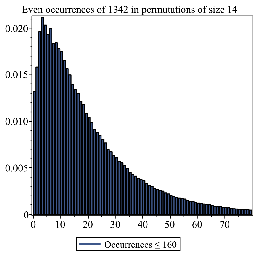
Figure 12: Histogram of 1234 even occurrences.

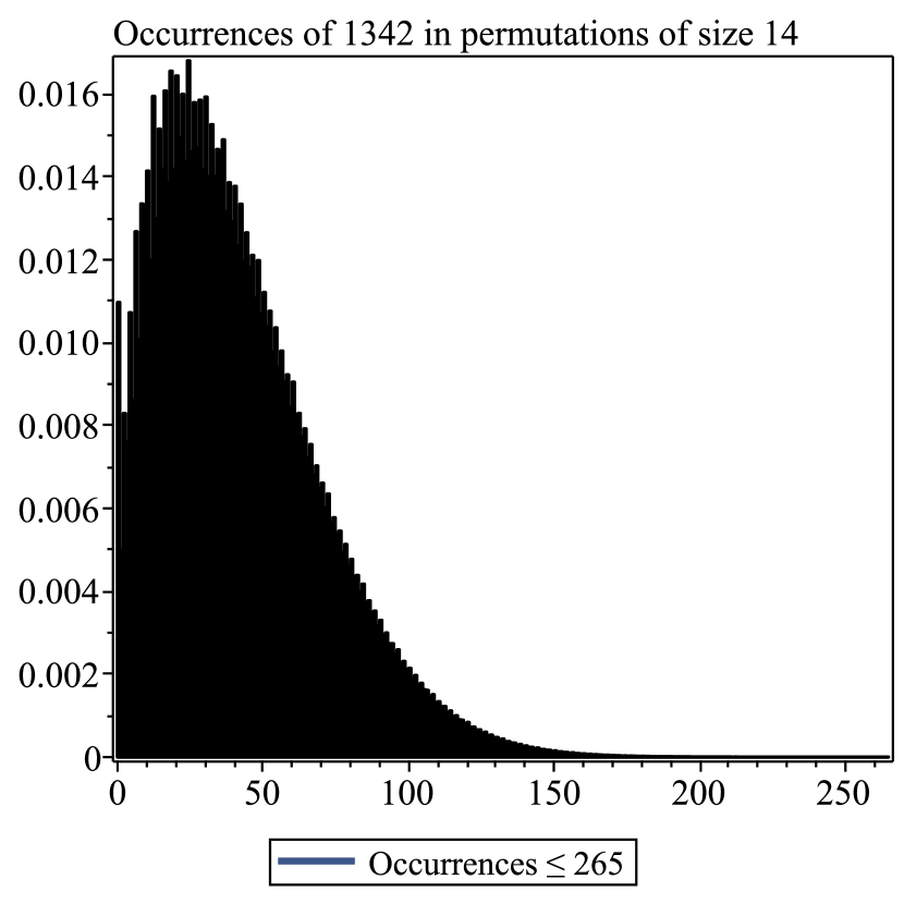
Figure 14: Histogram of 1342 occurrences.

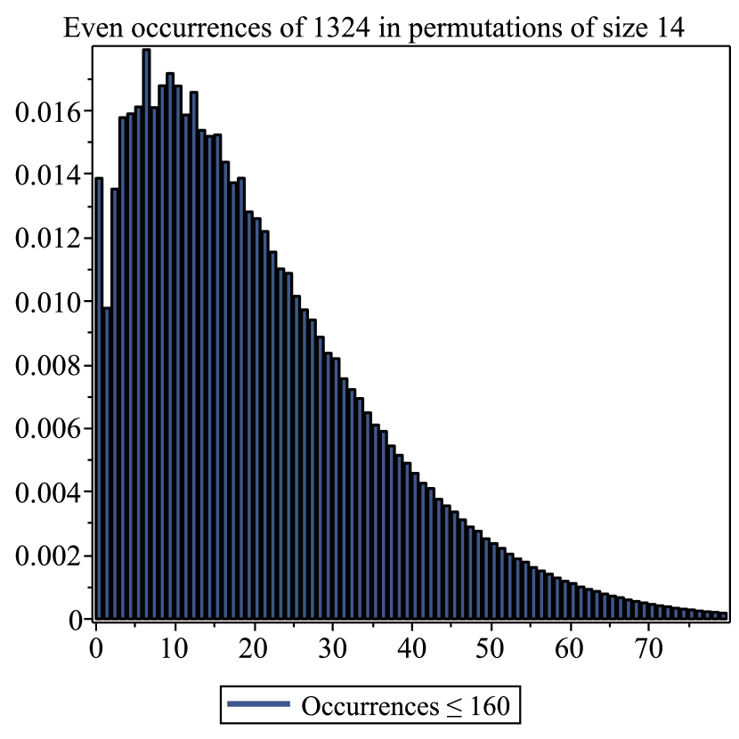
Figure 18: Histogram of 1324 even occurrences.

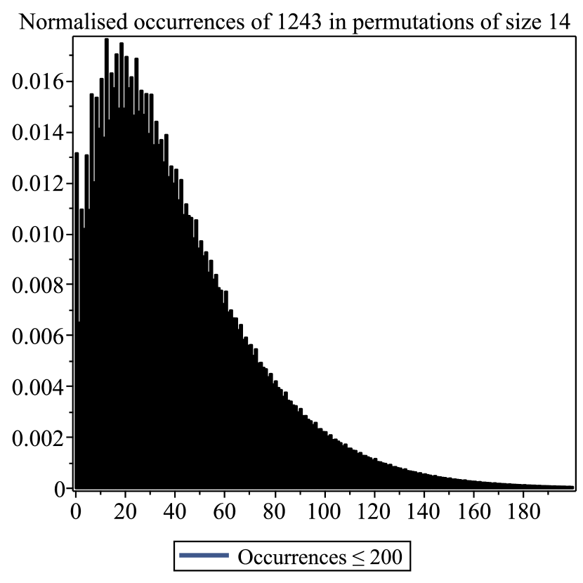
Figure 20: Histogram of 1243 occurrences.

We have shown in Figs. 12, 14, 18, 20 the normalised histograms for 4 of the 7 Wilf classes. The only reason we don’t show the histograms for the remaining 3 classes is that they provide no further illumination. Unlike the case for patterns of length 3, there appears to be an odd-even parity effect in every case, so we have also shown the odd- and even-subsequences for these four classes. Also unlike the situation for patterns of length 3, the histograms are quite skewed, compared to the comparatively symmetric shape (apart from the long, skinny tail) in the length-3 case.

As these distributions are provably asymptotically normal [28], the observed parity effects and asymmetry must be a manifestation of permutations that are too short. That is to say, we are far from the asymptotic regime.

Having observed the two different $r$-dependencies in the length-3 situation, we now investigate the corresponding asymptotics for the 7 length-4 Wilf classes.

5.1 Class I

As remarked above, for $r=1$ we have 200 terms, and for $r=2$ we have 25 terms. As we only have 17 terms for some of the classes that haven’t previously been studied, we will first confine our analysis to 17-term sequences, and then see if the additional terms change our conclusions. We will show our analysis in some detail for this case, and then apply exactly the same methods in all subsequent cases, and just quote the results.

As our analysis will be based on the ratio method and its extensions, as described in the appendix, it would be useful to have as many terms as possible, even if these terms are only approximate.

The method of series extension [17] allows us to predict additional terms by constructing holonomic differential equations from the known coefficients – known as the method of differential approximants [19] – and using these to predict further terms. This method is also briefly described in the appendix. By this method the accuracy of the predicted terms is assessed by constructing the variance of the estimates of each predicted coefficients, which we are able to do as we construct many distinct differential equations by varying the degrees of the polynomials multiplying the various derivatives. We cut off the number of predicted terms when the error grows larger than some desired maximum.

In this case we were able to predict 12 further coefficients, as shown in Table 1 below, where for comparison we have also shown the exact coefficients. It can be seen that the first predicted coefficient is in error by 1 part in the 9th significant digit, while the last predicted coefficient is in error by 6 parts in the 6th significant digit. These approximate coefficients are still useful for our analysis, as we now show.

Recall that for the pattern 123 the asymptotics did not change with the number of occurrences, only the amplitude did. We know that the exponential growth does not change, so the only possible change is in the power-law exponent. Recall that $\psi_{0}(n)\sim\frac{81\sqrt{3}\cdot 9^{n}}{16\pi\cdot n^{4}},$ see A005802 [42]. So $\psi_{1}(n)\sim\frac{C_{1}\cdot 9^{n}}{16\pi\cdot n^{g}},$ where $C_{1}$ and the exponent $g$ are unknown. If $g=4,$ then the ratio

$$\frac{\psi_{0}(n)}{\psi_{1}(n)}\sim\frac{81\sqrt{3}}{C_{1}\cdot n^{4-g}}$$

should tend to a non-zero constant $81\sqrt{3}/C_{1}$ as $n$ increases. Otherwise the ratio should diverge or vanish, according as $g$ is less than or greater than 4. It can be seen from Fig. 6 that the ratio is certainly not diverging, but rather appears to be going to a constant. We can also use the ratio method to estimate the value of $g$ directly, as the ratios $r_{n}=\psi_{1}(n)/\psi_{1}(n-1)\sim 9(1-g/n+o(1/n)).$ We estimate the exponent $g$ from the estimators $g_{n}=(r_{n}/9-1)n\sim-g(1+o(1)).$

In Fig. 6 we plot the estimators $g_{n}$ against $1/n.$ These are seen to be going to a value close to -4, though possibly a little lower. If the singularity is a pure power-law singularity, the sub-dominant term $o(1)$ is in fact $O(1/n).$ We can eliminate this term by forming the quadratic estimators $q_{n}\equiv ng_{n}-(n-1)g_{n-1}\sim g(1-o(1/n)).$ In Fig. 8 we show these quadratic estimators plotted against $1/n^{2},$ and it can be seen that there is an upturn in the estimators away from -4.5 and toward the value -4. To show that this is not spurious, we show in Fig. 8 the same plot, but this time using 45 terms, which we have in this case, and which clearly shows that the limiting value -4 is quite compelling.

It remains to estimate the value of the amplitude $C_{1}.$ This is equivalent to estimating the limit of the plot shown in Fig. 6, which we can’t do with the 29 terms we have at our disposal. However if we now use all 200 known terms, then this ratio is clearly going to a limit around $0.5,$ as can be seen from Fig. 10. And in Fig. 10 we show quadratic estimators of the same ratio, plotted against $1/n^{2}.$ It is clear that the limit is plausibly 0.5, which implies that

$$\psi_{1}(n)\sim\frac{81\sqrt{3}\cdot 9^{n}}{32\pi\cdot n^{4}}.$$

Recall from the previous section that for the pattern 123 we have $\psi_{1}(n)/\psi_{0}(n)=3.$ For the pattern 1234 we conjecture that $\psi_{1}(n)/\psi_{0}(n)=1/2.$

For the 2-occurrence sequence, as noted above, we have 25 terms available. By the method of series extension we are able to obtain a further 40 approximate terms. We have analysed that sequence exactly as described above for the 1-occurrence sequence, and we find exactly the same asymptotics, except that the ratio $\psi_{2}(n)/\psi_{0}(n)\approx 1.$ So we conjecture that

$$\psi_{2}(n)\sim\psi_{0}(n)\sim\frac{81\sqrt{3}\cdot 9^{n}}{16\pi\cdot n^{4}}.$$

It seems reasonable to conjecture that $\psi_{r}(n)=\frac{C_{r}\cdot 9^{n}}{n^{4}}$ for all $r,$ just as is the case for the shorter pattern 123. That is to say, as $r$ changes, only the amplitude $C_{r}$ changes. The exponential growth remains (provably) the same, and the sub-dominant power law term is also (conjecturally) unchanged. The pre-multiplicative amplitude is also of course just conjectured, rather than proved.

Table 1: Predicted and exact coefficients of order 18 to 29

Order	Predicted	Exact
18	2.05621895e+12	2056218941678
19	1.53582968e+13	15358296210724
20	1.15469577e+14	115469557503753
21	8.73561640e+14	873561194459596
22	6.6477690e+15	6647760790457218
23	5.0871661e+16	50871527629923754
24	3.9134709e+17	391345137795371013
25	3.0255951e+18	3025568471613091692
26	2.3502067e+19	23501724670464335914
27	1.8337471e+20	183370520135071994536
28	1.4368444e+21	1436795093911521996331
29	1.1303753e+22	11303188383039278887124

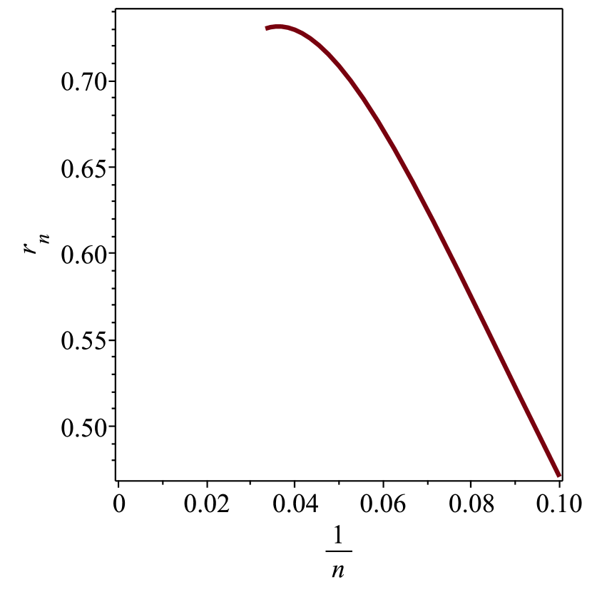
Figure 5: Ratio of $\psi_{1}(n)/\psi_{0}(n)$ plotted against $1/n$ for 1234 patterns.

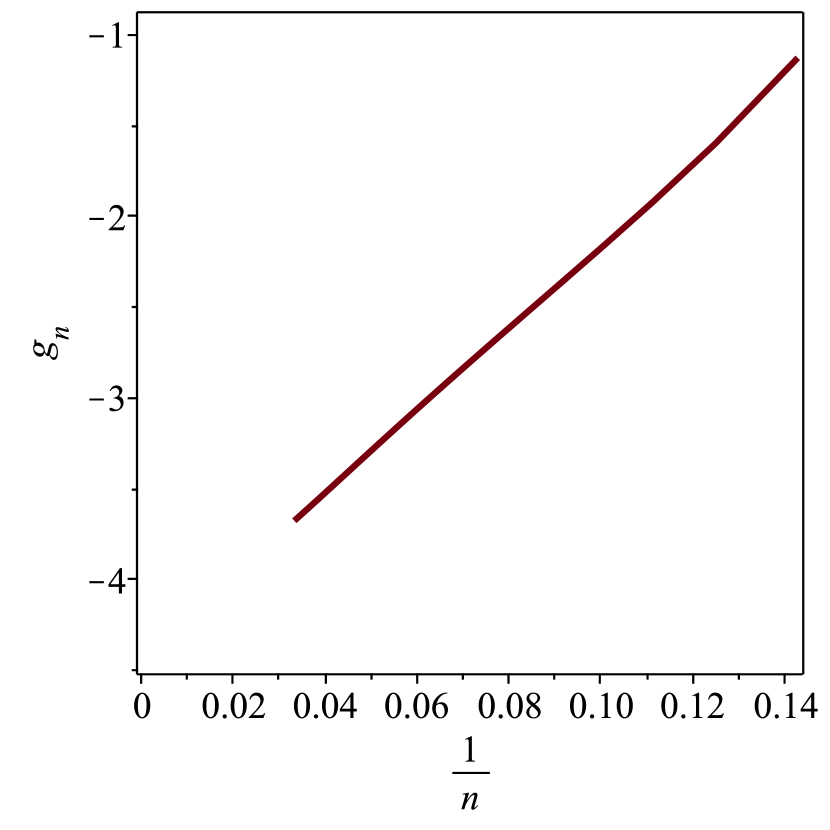
Figure 6: Estimators $g_{n}$ of exponent $g$ plotted against $1/n.$

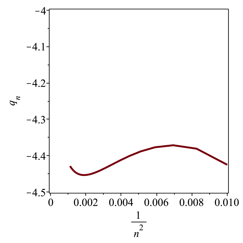
Figure 7: Quadratic estimators $q_{n}$ of exponent $g$ plotted against $1/n^{2},$ using 30 terms.

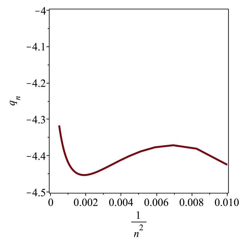
Figure 8: Quadratic estimators $q_{n}$ of exponent $g$ plotted against $1/n^{2},$ using 45 terms.

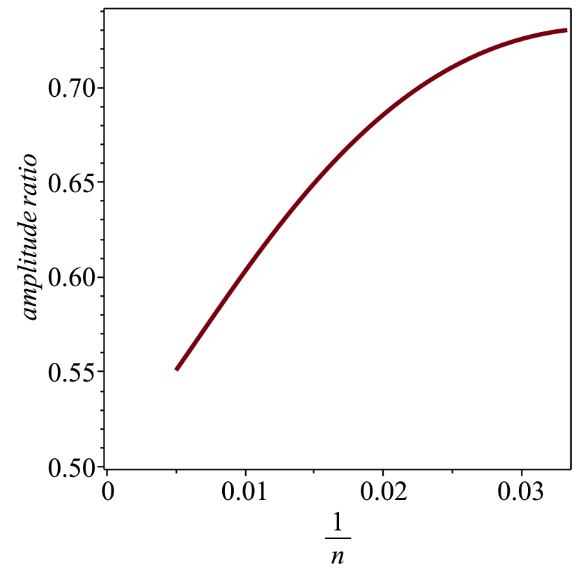
Figure 9: Amplitude ratios $\psi_{1}(n)/\psi_{0}(n)$ plotted against $1/n,$ using 200 terms.

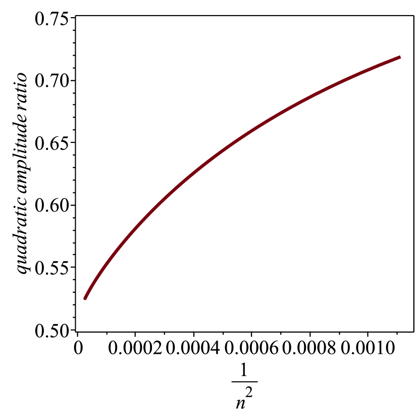
Figure 10: Quadratic amplitude ratios plotted against $1/n^{2},$ using 200 terms.

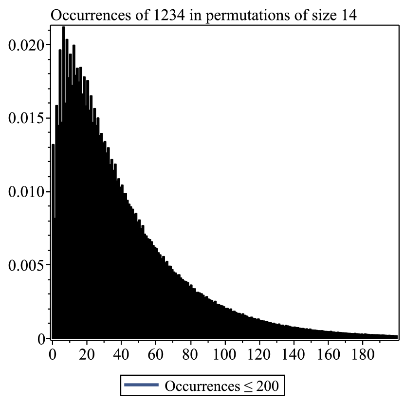
Figure 11: Histogram of 1234 occurrences.

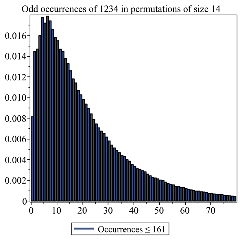
Figure 13: Histogram of 1234 odd occurrences.

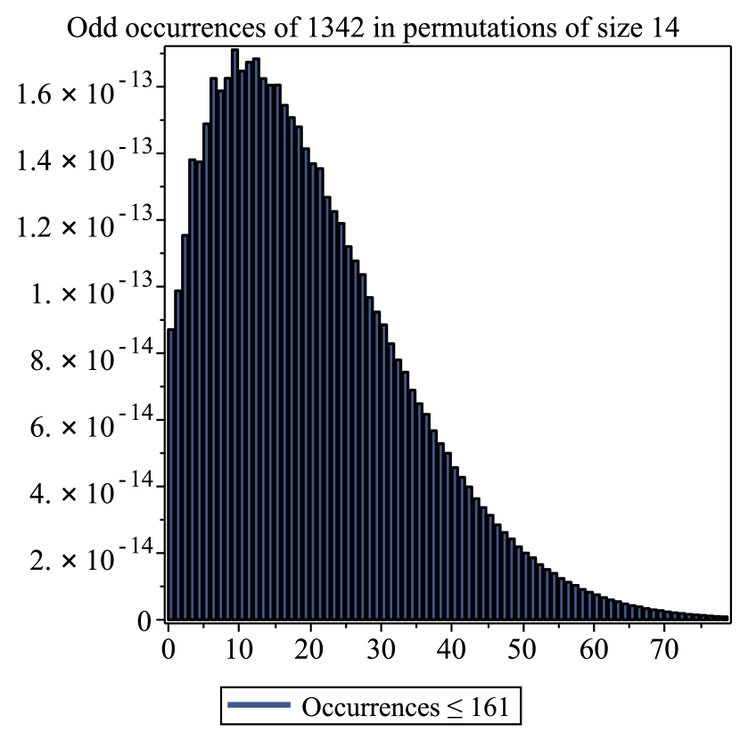
Figure 15: Histogram of 1342 odd occurrences.

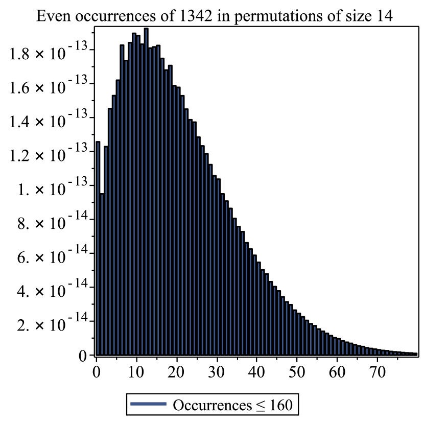
Figure 16: Histogram of 1342 even occurrences.

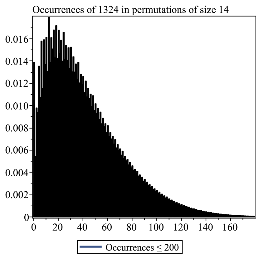
Figure 17: Histogram of 1324 odd occurrences.

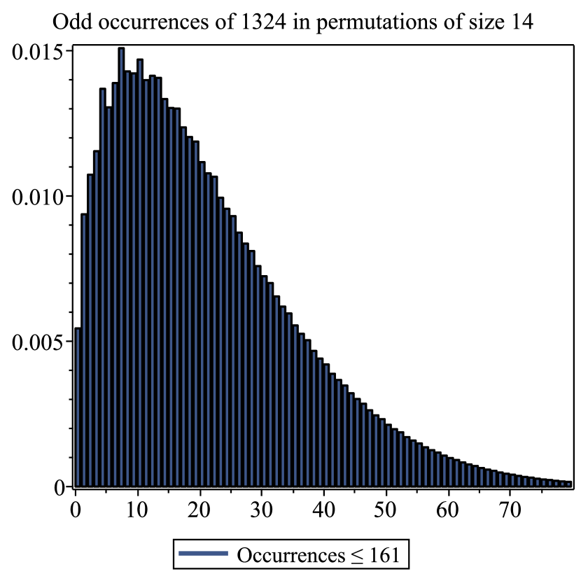
Figure 19: Histogram of 1324 odd occurrences.

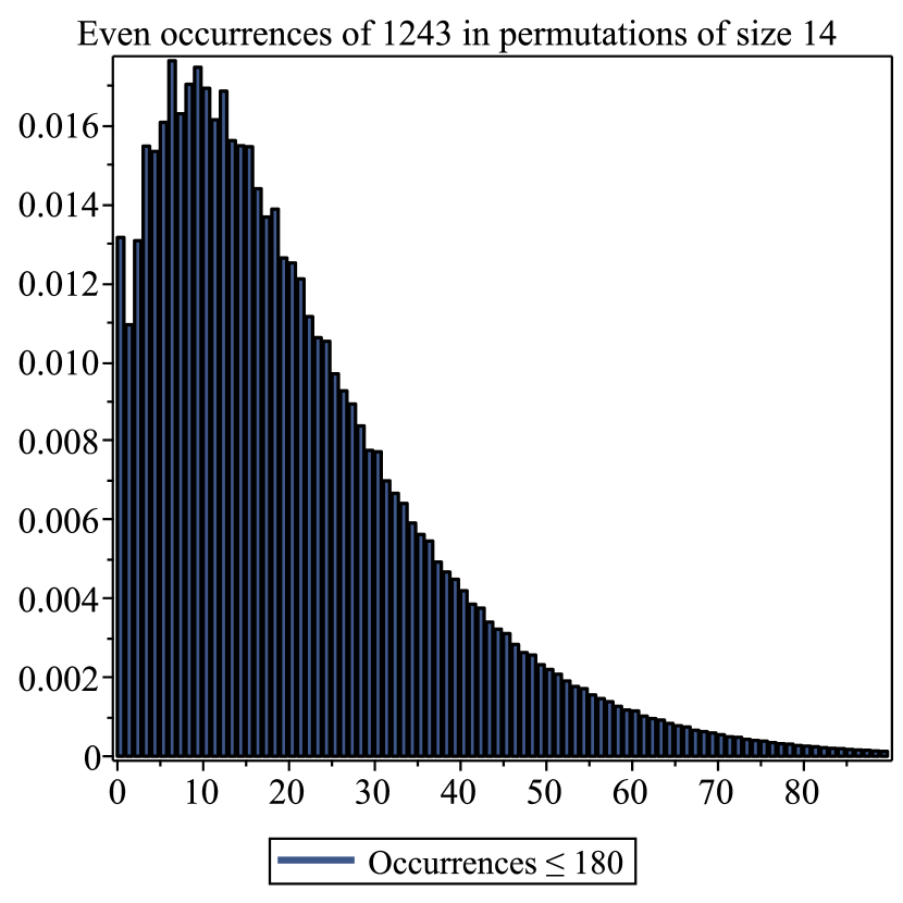
Figure 21: Histogram of 1243 even occurrences.

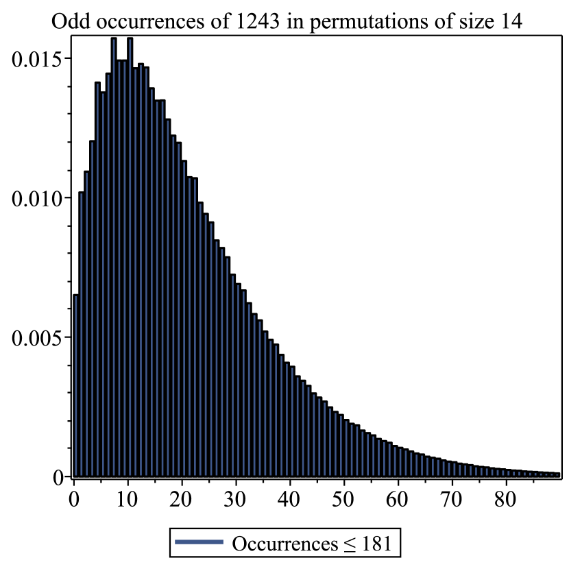
Figure 22: Histogram of 1243 odd occurrences.

5.2 Class II

We analysed OEIS sequence A224179 for 1-occurrences of the pattern 1243. 25 terms are given, and we were able to find a further 50 approximate terms with sufficient apparent accuracy for the ratio method to be used. We analysed this sequence in an identical manner to our analysis of 1234 1-occurrences, discussed in the previous section. The ratio $\psi(1243)_{1}(n)/\psi(1234)_{0}(n)$ is going to an apparent limit of $0.93125\pm 0.00015.$ If this were a simple fraction, $149/160=0.93125$ would seem to be a likely candidate.

Direct analysis of the coefficients of the sequence $\psi(1243)_{1}(n)$ for the power-law exponent also verified the O$(n^{-4})$ behaviour that follows from the fact that the ratio we have just estimated is non-zero and finite.

We conclude that $\psi_{1}(n)\sim\frac{C_{1}\cdot 9^{n}}{n^{4}},$ where $C_{1}\approx\frac{0.93125\cdot 81\sqrt{3}}{16\pi},$ and perhaps $C_{1}=149\cdot 3^{4}\sqrt{3}/(2^{9}\cdot 5\pi)$ exactly.

We similarly analysed the OEIS sequence A224181 for 2-occurrences of the pattern 1243. 24 terms are given, and we were able to find a further 40 approximate terms with sufficient apparent accuracy for the ratio method to be used. We analysed this sequence in an identical manner to our analysis of 1243 1-occurrences, just discussed. The ratio $\psi(1243)_{2}(n)/\psi(1234)_{0}(n)$ is going to an apparent limit of $2.93\pm 0.01.$ It is tempting to guess that this is just 2 greater than the corresponding ratio for the 1-occurrence case. If that were so, then a simple fraction, $469/160=2.93125$ would seem to be a likely candidate.

We conclude that $\psi_{2}(n)\sim\frac{C_{2}\cdot 9^{n}}{n^{4}},$ where $C_{2}\approx\frac{2.93\cdot 81\sqrt{3}}{16\pi},$ and perhaps $C_{2}=469\cdot 3^{4}\sqrt{3}/(2^{9}\cdot 5\pi)$ exactly.

As for the previous class, it seems reasonable to conjecture that $\psi_{r}(n)=\frac{C_{r}\cdot 9^{n}}{n^{4}}$ for all $r,$ just as is the case for the shorter pattern 123. That is to say, as $r$ changes, only the amplitude $C_{r}$ changes. The exponential growth remains (provably) the same, and the sub-dominant power law term is also (conjecturally) unchanged.

5.3 Class III

We analysed the OEIS sequence A224182 for 1-occurrences of the pattern 1432. 18 terms are given, and we were able to find a further 26 approximate terms with sufficient apparent accuracy for the ratio method to be used. We analysed this sequence in a similar manner to our analysis of 1234 1-occurrences, discussed above. However the ratio $\psi(1432)_{1}(n)/\psi(1234)_{0}(n)$ appears to be diverging linearly. Accordingly, we studied the sequence $\psi(1432)_{1}(n)/(n\cdot\psi(1234)_{0}(n)).$ That ratio is going to an apparent limit of $0.0375\pm 0.0005.$ It is tempting to guess that this is just $3/80.$

We conclude that $\psi_{1}(n)\sim\frac{C_{1}\cdot 9^{n}}{n^{3}},$ where $C_{1}\approx\frac{0.0375\cdot 81\sqrt{3}}{16\pi},$ and perhaps
$C_{1}=3^{5}\sqrt{3}/(2^{8}\cdot 5\pi)$ exactly.

We next analysed the sequence for 2-occurrences of the pattern 1432. We have generated 15 terms, and we were able to find a further 9 approximate terms with sufficient apparent accuracy for the ratio method to be used. We analysed this sequence in an identical manner to our analysis of 1432 1-occurrences, just discussed. The ratio $\psi(1432)_{2}(n)/(n^{2}\cdot\psi(1234)_{0}(n))$ is going to an apparent limit of $0.00075\pm 0.00005.$ This is too imprecise to hazard a guess at the exact value.

We conclude that

$$\psi_{2}(n)\sim\frac{C_{2}\cdot 9^{n}}{n^{2}},$$

where $C_{2}\approx\frac{0.00075\cdot 81\sqrt{3}}{16\pi}.$

We see that the behaviour of the $r$-occurrences is qualitatively similar to that of 132-avoiders, in that the power-law exponent increases by 1 as $r$ increases by 1. Accordingly, we conjecture that

$$\psi_{r}(n)\sim\frac{C_{r}\cdot 9^{n}}{n^{4-r}},$$

where $C_{0}$ is known, $C_{1}$ is conjectured, and $C_{2}$ is estimated.

5.4 Class IV

There is no pre-existing data for this class, of which 2143 is a representative member. We have generated 18 coefficients for $\psi_{1}(n)$ and 16 coefficients for $\psi_{2}(n).$ we were able to find a further 20 approximate terms for $\psi_{1}(n)$ and 15 approximate terms for $\psi_{2}(n)$ with sufficient apparent accuracy for the ratio method to be used.

We analysed these sequences in a similar manner to our analysis of other sequences, discussed above. The ratio $\psi(2143)_{1}(n)/\psi(1234)_{0}(n)$ again appears to be diverging linearly. Accordingly, we studied the sequence $\psi(2143)_{1}(n)/(n\cdot\psi(1234)_{0}(n)).$ That ratio is going to an apparent limit of $0.0421\pm 0.0005.$

We conclude that $\psi_{1}(n)\sim\frac{C_{1}\cdot 9^{n}}{n^{3}},$ where $C_{1}\approx\frac{0.0421\cdot 81\sqrt{3}}{16\pi}.$

We next analysed the sequence for 2-occurrences of the pattern 2143. We analysed this sequence in an identical manner to our analysis of 2143 1-occurrences, just discussed. The ratio $\psi(2143)_{2}(n)/(n^{2}\cdot\psi(1234)_{0}(n))$ is going to an apparent limit of $0.00090\pm 0.00005.$

We conclude that $\psi_{2}(n)\sim\frac{C_{2}\cdot 9^{n}}{n^{2}},$ where $C_{2}\approx\frac{0.0009\cdot 81\sqrt{3}}{16\pi}.$

We see that for this class too, the behaviour of the $r$-occurrences is qualitatively similar to that of 132-avoiders, in that the power-law exponent increases by 1 as $r$ increases by 1. Accordingly, we conjecture that

$$\psi_{r}(n)\sim\frac{C_{r}\cdot 9^{n}}{n^{4-r}},$$

where $C_{0}$ is known, and $C_{1}$ and $C_{2}$ are estimated.

5.5 Class V

For this class, of which 1324 is a representative member, 17 terms for $\psi_{1}(n)$ are given as OEIS sequence A224182, but there is no pre-existing data for $\psi_{2}(n).$ We have given 15 terms for that sequence. We have also used a further 15 and 8 approximate terms in our analysis, for 1- and 2-occurrences respectively.

Recall that for this class, uniquely, the result for 0-occurrences is not known rigorously. Numerical work by Conway et al. [9] suggests that $\psi_{0}(n)\sim C_{0}\cdot\mu^{n}\cdot\mu_{1}^{\sqrt{n}}\cdot n^{g},$ where $\mu\approx 11.598$ (and possibly $9+3\sqrt{3}/2$ exactly), $\mu_{1}\approx 0.0400,$ and $g\approx-1.1.$

Recall that $\psi_{r}(n)$ grows at the same rate as $\psi_{0}(n),$ so we studied the ratios

$$\psi_{r}(n)/\psi_{0}(n)$$

for $r=1$ and $r=2.$

The ratio $\psi(1324)_{1}(n)/\psi(1324)_{0}(n)$ appears to be diverging linearly. Accordingly, we studied the sequence $\psi(1324)_{1}(n)/(n\cdot\psi(1324)_{0}(n)).$ That ratio is going to an apparent limit of $0.013\pm 0.001.$

We conclude that

$$\psi_{1}(n)\sim C_{1}\cdot n\cdot\psi_{0}(n),$$

where $C_{1}=0.013\pm 0.001.$

For 2-occurrences, we studied the sequence $\psi(1324)_{2}(n)/(n^{2}\cdot\psi(1324)_{0}(n)).$ That ratio is going to an apparent limit of $0.0010\pm 0.0001.$ So we conclude that $\psi_{2}(n)\sim C_{2}\cdot n^{2}\cdot\psi_{0}(n),$ where $C_{2}=0.001\pm 0.0001.$

We see that for this class too, the behaviour of the $r$-occurrences is qualitatively similar to that of 132-avoiders, in that the power-law exponent apparently increases by 1 as $r$ increases by 1. Accordingly, we conjecture that

$$\psi_{r}(n)\sim C_{r}\cdot n^{r}\cdot\psi_{0}(n).$$

5.6 Class VI

For this class and class VII we have $\psi_{0}(n)\sim\frac{64\cdot 8^{n}}{243\sqrt{\pi}\cdot n^{5/2}}.$ There are no pre-existing sequences for any $r>0.$ For both classes we have generated 17 terms for 1-occurrences and 15 terms for 2-occurrences. We have also generated 30 approximate terms for 1-occurrences and 8 approximate terms for 2-occurrences, for both classes.

The ratio $\psi(1342)_{1}(n)/\psi(1342)_{0}(n)$ again appears to be diverging linearly. Accordingly, we studied the sequence $\psi(1342)_{1}(n)/(n\cdot\psi(1342)_{0}(n)).$ That ratio is going to an apparent limit of $0.0206\pm 0.0005.$

We conclude that

$$\psi_{1}(n)\sim\frac{C_{1}\cdot 8^{n}}{n^{3/2}},$$

where $C_{1}=0.0206\pm 0.0005.$

We analysed the sequence for 2-occurrences in an identical manner to our analysis of 1342 1-occurrences, just discussed. The ratio $\psi(1342)_{2}(n)/(n^{2}\cdot\psi(1342)_{0}(n))$ is going to an apparent limit of $0.0005\pm 0.0001.$ So we conclude that

$$\psi_{2}(n)\sim\frac{C_{2}\cdot 8^{n}}{n^{1/2}},$$

where $C_{2}=0.0005\pm 0.0001.$

5.7 Class VII

The ratio $\psi(2413)_{1}(n)/\psi(2413)_{0}(n)$ again appears to be diverging linearly. We again studied the sequence $\psi(2413)_{1}(n)/(n\cdot\psi(2413)_{0}(n)).$ That sequence is going to an apparent limit of $0.01463\pm 0.00005.$

We conclude that

$$\psi_{1}(n)\sim\frac{C_{1}\cdot 8^{n}}{n^{3/2}},$$

where $C_{1}=0.01463\pm 0.00005.$

We analysed the sequence for 2-occurrences in an identical manner to our analysis of 2413 1-occurrences, just discussed. The ratio $\psi(2413)_{2}(n)/(n^{2}\cdot\psi(2413)_{0}(n))$ is going to an apparent limit of $0.00010\pm 0.00002.$ So we conclude that

$$\psi_{2}(n)\sim\frac{C_{2}\cdot 8^{n}}{n^{1/2}},$$

where $C_{2}=0.00010\pm 0.00002.$

We see that for both class VI and class VII the behaviour of the $r$-occurrences is qualitatively similar to that of 132-avoiders, in that the power-law exponent apparently increases by 1 as $r$ increases by 1. Accordingly, we conjecture that

$$\psi_{r}(n)\sim C_{r}\cdot n^{r}\cdot\psi_{0}(n)$$

for both classes.

5.8 Class summary

Just as for patterns of length three, we see that the behaviour of $r$-occurrences of patterns of length four falls into two groups.

The first group consists of classes I and II. For those two classes, the asymptotic behaviour is unchanged as $r$ increases, and only the pre-multiplicative constant $C_{r}$ changes with $r$. That is to say, $\psi_{r}(n)\sim C_{r}\cdot\psi_{0}(n).$

For the second group, consisting of classes III-VII, the subdominant power-law behaviour changes, increasing by 1 with each unit increase in $r.$ It is also the case that the pre-multiplicative constant $C_{r}$ changes with $r$. That is to say, $\psi_{r}(n)\sim C_{r}\cdot n^{r}\cdot\psi_{0}(n).$

6 Stieltjes moment sequences

The classical Stieltjes moment problem considers a numerical sequence ${\bf a}\equiv\{a_{n}\},\,n\geq 0$ in which $a_{n}$ can be expressed as the integral

$$a_{n}=\int_{\Gamma}x^{n}d\rho(x)$$

for all $n\geq 0,$ where the support $\Gamma\subseteq{\mathbb{R}},$ and $\rho$ is a measure. If the measure $\rho$ is differentiable, then it has a density or density function $\mu(x)=\rho^{\prime}(x).$ In which case the above equation becomes

$$a_{n}=\int_{\Gamma}x^{n}\mu(x)dx.$$

There are several equivalent conditions that the sequence ${\bf a}$ must satisfy in order to be a Stieltjes moment sequence, or equivalently, for such a density function to exist, which must of course be non-negative.

The Hankel matrix $H_{n}^{\infty}({\bf a})$ is defined as

$$H_{n}^{\infty}({\bf a})=\begin{bmatrix}a_{n}&a_{n+1}&a_{n+2}&\ldots\\ a_{n+1}&a_{n+2}&a_{n+3}&\ldots\\ a_{n+2}&a_{n+3}&a_{n+4}&\ldots\\ \vdots&\vdots&\vdots&\ddots\\ \end{bmatrix}$$

The following theorem was proved in part by Stieltjes and in part by Gantmakher and Krein. In particular, the properties (a) and (d) (below) were shown to be equivalent by Stieltjes [47], while these were later shown to be equivalent to (b) and (c) by Gantmakher and Krein[13].

Theorem 1.

For a sequence ${\bf a}\equiv\{a_{n}\},\,n\geq 0$, the following are equivalent: (a) There exists a positive measure $\rho$ on $\Gamma\in[0,\infty)$ such that

$$a_{n}=\int_{\Gamma}x^{n}d\rho(x).$$

(b) The matrices $H_{0}^{\infty}({\bf a})$ and $H_{1}^{\infty}({\bf a})$ are both positive semidefinite.
(c) The matrix $H_{0}^{\infty}({\bf a})$ is totally positive (all of its minors are non-negative).
(d) There exists a sequence of real numbers $\alpha_{0},\,\alpha_{1},\ldots\geq 0$ such that the generating function $A(x)$ for the sequence $a_{0},a_{1},\ldots$ satisfies

$$A(x)=\sum_{n=0}^{\infty}a_{n}x^{n}=\cfrac{\alpha_{0}}{1-\cfrac{\alpha_{1}x}{1-\cfrac{\alpha_{2}x}{\begin{array}[]{@{}c@{}c@{}c@{}}1-\ldots\end{array}}}}$$

A sequence that satisfies the equivalent conditions of Theorem 1 is called a Stieltjes moment sequence.

One reason for attempting to identify combinatorial sequences as Stieltjes moment sequences is that such sequences are log-convex.

Log-convexity of the sequence ${\bf a}$ implies that the ratios $\frac{a_{n}}{a_{n-1}}$ provide lower bounds to the growth constant $\mu$ of the sequence. In the case that ${\bf a}$ is a Stieltjes moment sequence, we can use the above properties to compute stronger lower bounds for $\mu,$ using a method first given by Haagerup, Haagerup and Ramirez-Solano [21].

Using the coefficients $a_{0},a_{1},\ldots a_{n},$ we calculate the terms $\alpha_{0},\alpha_{1},\ldots\alpha_{n}$ in the continued fraction representation above. It is easy to see that the coefficients of $A(x)$ are non-decreasing in each $\alpha_{j}.$ Hence $A(x)$ is (coefficient-wise) bounded below by the generating function $A_{n}(x)$, defined by setting $\alpha_{n},\alpha_{n+1},\alpha_{n+2},\ldots$ to 0. Therefore, the growth rate $\mu_{n}$ of $A_{n}(x)$ is no greater than the growth rate $\mu$ of $A(x).$ The growth rates $\mu_{1},\mu_{2},\ldots$ clearly form a non-decreasing sequence, and, since the coefficients of $A_{n}(x)$ are log-convex, $\mu_{n}\geq a_{n}/a_{n-1}$. It follows that this sequence $\mu_{1},\mu_{2},\ldots$ of lower bounds converges to the exponential growth rate $\mu$ of a.

Bostan et al. [7] showed that for all known PAP generating functions, the coefficients were SMSs, and for Av(1324) the Hankel determinants were monotonically increasing with the determinant size, leading them to confidently conjecture that it too was a SMS. However for $r$-occurrences of patterns, for all patterns and for all $r>0$ we have investigated, none are SMSs.

Blitvíc and Steingrímmson [6] however suggested the following: For a given pattern of length $m,$ form the generating function $G(q),$ with coefficients

$$g_{n}=\sum_{k=0}^{\binom{m}{n}}q^{k}\psi_{k}(n).$$

Then ask for what values of $q,$ which we call $q_{c},$ do these coefficients form a Stieltjes moment sequence? Clearly it is true for $q=0,$ as that corresponds to the the observation that the ogf for PAPs is an SMS. For $q>0$ the Hankel determinants, observationally, become larger as $q$ becomes larger. So this only leaves $q<0$ to explore.

For patterns of length $m=3$ the answer appears to be for $q_{c}=0.$ That is, the Hankel determinants are negative for $q<0.$ For patterns of length $m=4$ the answer appears to be $q_{c}<0,$ and is possibly pattern dependent. We experimentally determine the value of $q=q_{c}(n)$ for which the Hankel determinant of size $n\times n$ first becomes negative. In fig. 24 and fig. 24 we show $q_{c}(n),$ the maximum value of $q$ for which the Hankel determinants are positive, for the two Wilf classes of length 3. We plot these against $1/n,$ and it can be seen that these maxima are monotonically increasing with $n,$ and visually extrapolate to a value indistinguishable from 0. On the other hand, in figs. 26, fig. 26 and fig. 27, for the patterns $1234,$ $1243$ and $1324$ respectively, while the maxima are again monotonically increasing with $n,$ visual extrapolation suggest a value of $q_{c}$ less than zero.

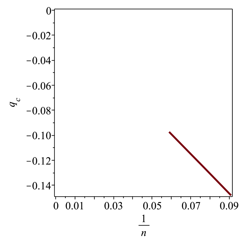
Figure 23: For 123, $q_{c}$ plotted against $1/n,$ where Hankel determinant is $n\times n.$

Figure 24: For 132, $q_{c}$ plotted against $1/n,$ where Hankel determinant is $n\times n.$

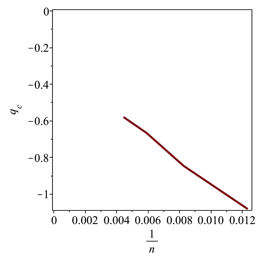
Figure 25: For 1234, $q_{c}$ plotted against $1/n,$ where Hankel determinant is $n\times n.$

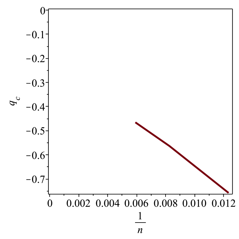
Figure 26: For 1243, $q_{c}$ plotted against $1/n,$ where Hankel determinant is $n\times n.$

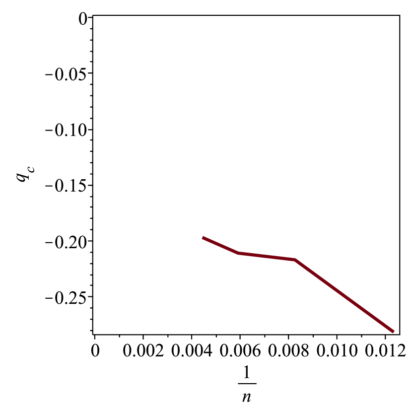
Figure 27: For 1324, $q_{c}$ plotted against $1/n,$ where Hankel determinant is $n\times n.$

7 Conclusion

We have given details of a new algorithm for enumerating multisets that is likely to be of broad applicability. As a first application, we have studied the behaviour of occurrences of patterns in permutations. For patterns of length 3 we give the general solution for the two Wilf classes, and have given the first systematic study of patterns of length 4, based on extensive enumerations obtained from our algorithm, combined with some longer enumerations obtained by others in isolated special cases. We find that there are seven Wilf classes, and have given conjectured asymptotic formulae for the behaviour of each of these classes.

8 Acknowledgements

We are particularly grateful to Yuma Inoue who modified his program for counting PAPs to counting occurrences of patterns, and using his program we were able to provide verification of the results produced by our program, and in a couple of specific cases obtain an additional term in the sequence. We are also grateful to Natasha Blitvić and Einar Steingrímsson for informative discussions about their interesting measure posed in their paper [6]. We would also like to thank Doron Zeilberger for helpful comments on the manuscript.

References

- [1] M Bóna, The number of permutations with exactly 132-subsequences is P-recursive in the size!, Adv. Appl. Math. 18, 510-522 (1997).
- [2] M Bóna, Exact enumeration of 1342-avoiding permutations: a close link with plane trees and planar maps, J Combin Theory Ser A 80(2) 257–272, (1997).
- [3] M Bóna, Permutations with one or two 132-subsequences,, Disc. Math. 181, 267-274, (1998).
- [4] M Bóna, On three different notions of monotone subsequences, arXiv:0711.4325v1, (2007).
-
[5]
M Bóna, The copies of any permutation pattern are asymptotically normal,
arXiv:0712.2792v1, (2007). - [6] N. Blitvić and E Steingrímsson, (More on) Combinatorial moment sequences and permutation patterns, Pattern Avoidance, Statistical Mechanics and Computational Complexity, Dagstuhl Reports, 13, issue 03 (to appear).
- [7] A Bostan, A Elvey Price, A J Guttmann, J-M Maillard, Stieltjes moment sequences for pattern-avoiding permutations, Elec. J. Combin., 27, (4) p4.20 (2020).
- [8] ,D Callan, A recursive bijective approach to counting permutations containing 3-letter patterns, arXiv:math/0211380v1, (2002).
- [9] A R Conway, A J Guttmann and P Zinn-Justin, 1324-avoiding permutations revisited, Adv. in Appl. Math. 96 312-333 (2018).
- [10] P Flajolet and R Sedgewick, Analytic Combinatorics, Cambridge UP, Cambridge, 2009.
- [11] A R Forsyth, Part III, Ordinary linear equations, vol. IV of Theory of differential equations Cambridge UP, (Cambridge), (1902).
- [12] M Fulmek, Enumeration of permutations containing a prescribed number of occurrences of a pattern of length 3, arXiv:math/0112092v3 (2002).
- [13] F Gantmakher and M Krein, Sur les matrices completement non négatives et oscillatoires, Compositio Mathematica 4 445-476, (1937).
- [14] S Garrabrant and I Pak, Words in linear groups, random walks, automata and P-recursiveness, J. Comb. Alg. 1(2) 127–144, (2017).
- [15] I Gessel, Symmetric functions and -recursiveness, J Combin Theory Ser A, 53(2) 257–285, 1990.
- [16] A J Guttmann, Analysis of series expansions for non-algebraic singularities, J. Phys A:Math. Theor. 48 045209, (33pp) (2015).
- [17] A J Guttmann, Series extension: predicting approximate series coefficients from a finite number of exact coefficients, J. Phys A:Math. Theor. 49 415002, (27pp) (2016).
- [18] A J Guttmann, in Phase Transitions and Critical Phenomena, vol 13, eds. C Domb and J Lebowitz, Academic Press, London and New York, 1989.
- [19] A J Guttmann and G S Joyce, A new method of series analysis in lattice statistics, J Phys A, 5 L81– 84, (1972).
- [20] A J Guttmann and I Jensen Series Analysis. Chapter 8 of Polygons, Polyominoes and Polycubes Lecture Notes in Physics 775, ed. A J Guttmann, Springer, (Heidelberg), 2009.
- [21] S Haagerup, U Haagerup and M Ramirez-Solano, A computational approach to the Thompson group F, Int. J. Alg. and Comp. 25 381-432, (2015).
- [22] L Hofer, A central limit theorem for vincular permutation patterns, Disc. Math. and Theor. Comp. Sci. 19:2, 2018, #9. See also arXiv:1704.00650v4
-
[23]
Y Inoue, Studies on Permutation Set Manipulation based on Decision Diagrams, Doctor of Info. Sciences thesis, Hokkaido University, (2017).
https://eprints.lib.hokudai.ac.jp/dspace/handle/2115/65366?locale=en&lang=en - [24] Y Inoue, Paper in preparation, (2022).
- [25] Y Inoue, T Toda and S Minato, Implicit generation of pattern-avoiding permutations based on DD, TCS Technical Report TCS-TR-A-13.67, Hokkaido Univ. (2013).
- [26] Y Inoue and S Minato, An Efficient Method for Indexing All Topological Orders of a Directed Graph, ISAAC 2014 Conference Proceedings, H.-K Ahn and C.-S Shin (Eds.) 103-114, (2014)
- [27] E L Ince, Ordinary differential equations, Longmans, Green and Co, (London), 1927.
- [28] S Janson, B Nakamura and D Zeilberger, On the asymptotic statistics of the number of occurrences of multiple permutation patterns, arXiv:1312.3955v1 (2013).
- [29] F Johansson and B Nakamura, Using functional equations to enumerate 1324-avoiding permutations, arXiv:1309.7117v1 (2013).
- [30] S Kitaev, Patterns in permutations and words, Springer, Heidelberg, (2011).
- [31] D E Knuth, The Art of Computer Programming, Vol. 4 Fascicle 1, Bitwise Tricks and Techniques, Binary Decision Diagrams, Addison-Wesley NJ (2009)
- [32] W Kuszmaul, Fast algorithms for finding pattern avoiders and counting pattern occurrences in permutations, Math. Comp. 87 987-1011, (2018). .
-
[33]
T Mansour, R Rastegar and A Roitershtein, Finite automata, probabilistic method, and occurrence enumeration of a pattern in words and permutations,
arXiv:1905.05646, (2019). - [34] T Mansour and A Vainshtein, Counting occurrences of 132 in a permutation, Adv. in Appl. Math. 28, 185-195 (2002)
- [35] A Marcus and G Tardos, Excluded permutation matrices and the Stanley-Wilf conjecture, J. Comb. Theor. A 107(1) 153-160, (2004)
- [36] Shin-ichi Minato, Zero-suppressed BDDs for set manipulation in combinatorial problems, 30th Design Automation Conference, pp 272–277. ACM Press, (1993).
- [37] Shin-ichi Minato. DD: A New Decision Diagram for Efficient Problem Solving in Permutation Space, Theory and Applications of Satisfiability Testing - SAT 2011 - 14th International Conference, SAT 2011, Ann Arbor, MI, USA, (2011). Proceedings, vol. 6695 of Lecture Notes in Computer Science, pp 90–104. Springer, Berlin, Heidelberg, (2011).
- [38] B Nakamura, Approaches for enumerating permutations with a prescribed number of occurrences of patterns, arXiv:1301.5080v2 (2013).
- [39] B Nakamura and D Zeilberger, Using Noonan-Zeilberger functional equations to enumerate (in polynomial time!) generalized Wilf classes, Adv. Appl. Math. 50, 356–366 (2013).
- [40] J Noonan, The number of permutations containing exactly one increasing subsequence of length three, Disc. Math. 152, 307-313 (1996).
- [41] J Noonan and D Zeilberger, The enumeration of permutations with a prescribed number of "forbidden" patterns, Adv. Appl. Math. 17, 381-407 (1996).
- [42] OEIS Foundation Inc. (2014), The On-Line Encyclopaedia of Integer Sequences, http://oeis.org.
- [43] A Regev, Asymptotic values for degrees associated with strips of young diagrams, Adv. in Math. 41(2) 115–136, (1981).
- [44] A Reifegerste, A generalization of Simion-Schmidt’s bijection for restricted permutations Elec. J. Combin. 9(2) paper 14, 9 pp. (2002/03). Permutation patterns (Otaga, 2003).
- [45] Z Stankova and J West, A new class of Wilf-equivalent permutations. J. Alg. Combin. 15 271-290, (2002).
- [46] E Steingrímsson, Generalized permutation patterns – a short survey, in Permutation Patterns, eds. S Linton, N Ruskuc and V Vatter, London Math Soc Lecture Note Series 376, Cambridge, University Press, 2010.
- [47] T-J Stieltjes, Recherches sur les fractions continues, Annales de la Faculté des sciences de Toulouse: Mathématiques. 8 (4) 1122, (1894).
- [48] V. Vatter, Permutation Classes, in Handbook of Enumerative Combinatorics, ed. M. Bona, CRC Press, Boca Raton, Ch. 12 753–834, (2015).
- [49] E M Wright, The coefficients of a certain power series, J London Math Soc, 7 256–262, 1932.
- [50] E M Wright, On the coefficients of power series having exponential singularities, J London Math Soc, 24 304–309, 1949.
- [51] https://sites.math.rutgers.edu/~zeilberg/tokhniot/oF1234bManuelKauers