Mapping poverty at multiple geographical scales

Abstract

Poverty mapping is a powerful tool to study the geography of poverty. The choice of the spatial resolution is central as poverty measures defined at a coarser level may mask their heterogeneity at finer levels. We introduce a small area multi-scale approach integrating survey and remote sensing data that leverages information at different spatial resolutions and accounts for hierarchical dependencies, preserving estimates coherence. We map poverty rates by proposing a Bayesian Beta-based model equipped with a new benchmarking algorithm accounting for the double-bounded support. A simulation study shows the effectiveness of our proposal and an application on Bangladesh is discussed.

Keywords — Bayesian analysis, Beta regression, Demographic and Health Survey, Development economics, Small area estimation.

1 Introduction

The first goal of the 2030 Agenda for Sustainable Development of the United Nations is to eradicate poverty in all its forms. Given that, current research trends are focusing on the complexity, spatial heterogeneity, and geographical roots of poverty to properly design out-of-poverty paths (Allard and Allard, 2017; Fan and Cho, 2021; Zhou and Liu, 2022). Poverty has a multifaceted nature compounded by its spatial dimension (Gauci, 2005): as an example, we can mention that widely used classifications divide it into urban and rural poverty (Christiaensen and Todo, 2014). Moreover, the study of spatial poverty traps, theorized as a persistent poverty status caused by location characteristics, e.g., remoteness, poor infrastructure and services, and/or excessive migration costs (Kraay and McKenzie, 2014) has received considerable attention.

For these reasons, poverty mapping is sparking interest in welfare economics and geography studies (Jean et al., 2016; Hall et al., 2023), as an essential methodology to support the investigation of the spatial distribution and regional characteristics of poverty. In addition, if performed at a granular level, it enables a geographical targeting, namely the area-driven allocation of resources for poverty alleviation (Elbers et al., 2007; Liu et al., 2017). This is recognized as an effective and cost-saving tool for poverty reduction if compared to individual targeting as the latter is characterized by high administrative costs of data collection and follow-up. Conversely, regional targeting does not require household tracking, easing the supervision and management processes (Bigman and Fofack, 2000; Galasso and Ravallion, 2005). Furthermore, it enables the diversification of policy instruments employed from area to area that can be easily combined with other antipoverty measures.

When performing poverty mapping, a natural problem relates to the choice of the spatial scale which strictly depends on the purpose of the analysis. This adds up to a more technical problem that arises when aggregating areal data from neighboring zones. Indeed, such an aggregation induces a smoothing effect that can mask or distort information on spatial heterogeneity (patchiness) of the target poverty measure (e.g., see Figure 1). This is known in geography as the scaling problem, and represents one of the aspects of the Modifiable Area Unit Problem (MAUP, Kolaczyk and Huang, 2001; Pratesi and Salvati, 2016). This effect strongly depends on the heterogeneity of the aggregated areas and might lead to misleading conclusions. A simple strategy to deal with it is to undertake the analysis by using multiple scales at once (Kolaczyk and Huang, 2001).

The choice of the spatial scale is also strongly connected with the availability of data sources. In particular, surveys on income, consumption and/or living conditions are commonly used in poverty mapping but typically provide reliable estimates at high levels of spatial aggregation (e.g., regional or national). Survey estimates are increasingly unreliable when considering finer spatial levels, translating into smaller and smaller sample sizes (Pratesi and Salvati, 2016). In addition, remote sensing (RS) or mobile phone usage data are recently employed in poverty mapping, especially in developing countries (Jean et al., 2016; Schmid et al., 2017). As opposed to survey data, such alternative sources are highly informative at fine spatial levels, while losing power when aggregated.

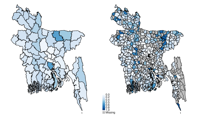
Figure 1: Poverty rate estimates at zila level (district) on the left-hand side and at upazila level (sub-district) on the right-hand side. Note that upazila level heterogeneity is masked when aggregating at the zila level.

A good practice in poverty mapping is to promote the efficient integration of multiple sources by means of statistical models (Steele et al., 2017; Zhao et al., 2019). To do so, we have to optimize the informative power that distinct sources have at different scales while accounting for hierarchical dependencies among levels. In this sense, a multi-scale procedure enables such an integration, while overcoming the aforementioned scaling problem. To the best of our knowledge, no explicit formalization of a multi-scale modeling approach has been proposed in the poverty mapping literature. Some proposals exploit geo-statistical models to obtain a continuous surface estimation over the study area (Puurbalanta, 2021; Sohnesen et al., 2022), avoiding the scaling problem. Such methods, however, require the exact location of each household which is difficult to obtain due to data disclosure restrictions.

We propose a Bayesian multi-scale model for poverty mapping that combines survey and alternative sources, available at both finer and coarser spatial levels, and does not require the exact location of survey respondents. The quantity we target is a poverty rate, defined as the proportion of people whose income or living conditions indicator falls below a pre-specified threshold. Our methodology sets in the framework of the Small Area Estimation (SAE) literature, aiming at estimating population quantities in areas (or domains) not originally planned by the survey design (Tzavidis et al., 2018; Rao and Molina, 2015, Ch. 4), where area-specific sample sizes are likely to be too small to yield precise enough estimates, or even null. SAE methods have been widely used in poverty mapping (Molina et al., 2014; Casas-Cordero Valencia et al., 2016; Corral et al., 2022; Bikauskaite et al., 2022), and most of them rely on models defined at the unit level. Conversely, we adopt an area-level approach, namely integrating the area direct estimates with areal covariates. We remark that this approach requires neither survey microdata nor covariates defined for the entire population.

In this paper, poverty rates are modeled through a Beta-based model (Liu et al., 2014; Fabrizi et al., 2016b; Janicki, 2020). Specifically, we rely on the Extended Beta proposed in De Nicolò et al. (2022). Its features solve major issues encountered in poverty mapping such as the double-bounded support of poverty measures, the excess of zero/one values, and the intra-cluster correlation induced by the survey design. A new methodology to assess the uncertainty associated with out-of-sample areas is also proposed. We extend it to deal with multiple spatial scales, enabling us to overcome the scaling problem as well as to efficiently integrate multiple sources; in doing so, we provide a fresh contribution to poverty mapping literature.

Previous proposals that deal with multiple levels in SAE convey information in a single direction: from finer to coarser as the so-called sub-area or two-fold models (Torabi and Rao, 2014; Erciulescu et al., 2019), or from coarser to finer through geo-statistical models (Benedetti et al., 2022). Our proposal, instead, leverages the information streams in both directions by considering multiple predictors with shared random effects, introducing in the poverty mapping framework the approach proposed by Aregay et al. (2016, 2017) in the disease mapping literature.

A multi-scale approach must ensure the coherence of poverty estimates across levels: poverty rate estimates at a given low-resolution area must correspond to the population-weighted aggregation of higher-resolution area estimates. The misalignment among estimates obtained at multiple levels is settled by the so-called benchmarking techniques (Bell et al., 2013), reviewed in Section 4. Conventional benchmarking methods do not account for the bounded support of poverty rates and may return invalid outcomes, possibly lying below zero or above one. We propose a new benchmarking procedure that suitably restricts the parameter space to the unit interval and relies on the idea of posterior projection (Dunson and Neelon, 2003; Sen et al., 2018). This represents a contribution to the literature as it provides benchmarked estimates and related uncertainty measures that are fully consistent with the bounded support.

Our proposal of multi-scale modeling equipped with a suitable benchmarking procedure is applied to map poverty in Bangladesh at two different spatial layers: zilas, i.e. administrative districts, and upazilas, i.e. sub-districts comparable with counties or boroughs. We use data from the Bangladesh Demographic and Health Survey (DHS; Fabic et al., 2012) by considering as poverty measure the proportion of people in the area falling in the first quintile of the national distribution of the Wealth Index (WI; Pirani, 2014). WI is a composite score that summarizes the living conditions of a household and that can be read as a measure of socioeconomic status (Poirier et al., 2020). The insufficient survey sample sizes in most zilas and upazilas (one-third of the upazilas are out-of-sample) drive us to integrate survey with RS data. Open access RS data encompasses night light radiance, population structure and population density, along with geographical characteristics, land use, infrastructures, and other social and economic features known to be poverty predictors at granular levels (Zhou and Liu, 2022). Eventually, we compare the performance of our multi-scale model to alternatives by means of a design-based simulation study.

The paper is organized as follows. Section 2 introduces the notation; Section 3 is devoted to a detailed description of the proposed small area model defined at multiple levels, prior specification, and posterior inference algorithms, along with a review of other standard models. The benchmarking proposal is illustrated in Section 4. Section 5 presents a design-based simulation exercise that tests the performance of our model in comparison with alternatives. An application of poverty mapping in Bangladesh by using DHS and RS data is illustrated in Section 6. Conclusions are drawn in Section 7.

2 Notation and survey-based estimators

The statistical models discussed afterward primarily rely on survey data. In this section, we introduce the notation and basic survey quantities, such as the poverty rate estimators and related uncertainty measure, which constitutes the starting point of our modeling framework. Let $\mathcal{U}$ denotes a finite population of $N$ individuals, on which we define two nested partitions, although the following setting can be easily generalized to multiple partitions. The first partition divides $\mathcal{U}$ into $D$ non-overlapping domains $\mathcal{U}_{d}$ at a coarser level, labeled as areas, each constituted by $N_{d}$ units. A second partition at a finer level divides each $\mathcal{U}_{d}$, $d=1,\dots,D$, into $M_{d}$ sub-areas $\mathcal{U}_{dj}$ of size $N_{dj}$, so that $M=\sum_{d=1}^{D}M_{d}$ is the overall number of sub-areas.

A complex survey sample of overall size $n$ is drawn from $\mathcal{U}$ and, on its turn, it can be partitioned into area and sub-area sub-samples of sizes $n_{d}$ and $n_{dj}$, $\forall d,j$ respectively. The notations $\hat{\bar{Y}}_{d}$ and $\hat{\bar{Y}}_{dj}$ denote the estimators based on survey data (direct estimators) of a poverty rate for areas $d=1,\dots,D$ and the nested sub-areas $j=1,\dots,M_{d}$, respectively. Let $w_{dji}$ denotes the sampling weight of individual $i=1,\dots,n_{dj}$ pertaining to area $d$ and sub-area $j$, and $y_{dji}$ the indicator variable denoting the poverty status. As our target domains are not planned in the survey design, we employ an Hájek-type estimator (Hájek, 1971) defined as

$$\hat{\bar{Y}}_{dj}=\frac{\sum_{i=1}^{n_{dj}}w_{dji}y_{dji}}{\sum_{i=1}^{n_{dj}}w_{dji}},\quad j=1,\dots,M_{d},\ d=1,\dots,D$$ (1)

$$\hat{\bar{Y}}_{d}=\frac{\sum_{j=1}^{M_{d}}\sum_{i=1}^{n_{dj}}w_{dji}y_{dji}}{\sum_{j=1}^{M_{d}}\sum_{i=1}^{n_{dj}}w_{dji}}=\frac{\sum_{j=1}^{M_{d}}\left(\sum_{i=1}^{n_{dj}}w_{dji}\right)\hat{\bar{Y}}_{dj}}{\sum_{j=1}^{M_{d}}\sum_{i=1}^{n_{dj}}w_{dji}}.$$ (2)

Those estimators are approximately unbiased for the unknown population proportions denoted with $\theta_{d}$ and $\theta_{dj}$, assuming that $0<\theta_{d}<1$ and $0<\theta_{dj}<1$. Defining as $t$ the national poverty rate and as $s_{d}=N_{d}/N$ the known population share, it holds that $\sum_{d=1}^{D}s_{d}\theta_{d}=t$. Furthermore, the sub-area partition implies

$$\sum_{j=1}^{M_{d}}s_{dj}\theta_{dj}=\theta_{d},\quad d=1,\dots,D,$$ (3)

where $s_{dj}=N_{dj}/N_{d}$ with $\sum_{d}s_{d}=\sum_{j}s_{dj}=1$.

Survey estimates from (1) and (2) may be highly imprecise due to the small sample sizes. To assess the reliability of estimates, we need to introduce a measure of uncertainty, included also in the modeling framework of Section 3. To account for the complex design, we focus on the effective sample sizes $\tilde{n}_{d}$ and $\tilde{n}_{dj}$, i.e. the virtual sample sizes required by a simple random sample to retrieve estimators with standard errors equal to those of $\hat{\bar{Y}}_{d}$ and $\hat{\bar{Y}}_{dj}$, obtained under complex design. Focusing on the area case, we can express the sampling variance of $\hat{\bar{Y}}_{d}$ as $\theta_{d}(1-\theta_{d})\tilde{n}_{d}^{-1}$, being the estimator of a proportion. The equivalent sample sizes incorporate the gains and losses in efficiency due to stratification, weighting, and the possibly strong intra-cluster correlation. They can be expressed in terms of the design effect DEff_d, i.e. the ratio between the variance of the direct estimator and its variance under simple random sampling, as $\tilde{n}_{d}=n_{d}/\text{DEff}_{d}$. The same reasoning applies for $\hat{\bar{Y}}_{dj}$. We remark that, given the different correlation structures occurring within areas and sub-areas, generally $\tilde{n}_{d}\neq\sum_{j=1}^{M_{d}}\tilde{n}_{dj}$.

The estimated uncertainty measures allow the detection of spatial levels with unreliable estimates, thus requiring SAE techniques. In our framework, two different spatial levels are considered and we assume that they both present unreliable estimates as surveys are generally planned for national (or regional) aggregates.

3 Small Area Models

Among SAE techniques, we focus on models defined at the area level. Small area models may be also defined at the unit (or individual) level and generally requires the individual auxiliary information to be known for the entire population. As novel data sources, such as RS data, provide areal information, the area-level models seem particularly suitable for poverty mapping.

We consider a hierarchical Bayesian model for proportions based on an extended Beta distribution, introduced in De Nicolò et al. (2022), by extending it for multiple spatial scales. We recall its single-level specification in Section 3.1, whereas multi-level specifications follow in Section 3.2.

3.1 The extended Beta model

The extended Beta (EB) model is defined as a mixture of a Beta distribution and two Dirac components defined on the boundaries 0 and 1 (Fabrizi et al., 2016a; Janicki, 2020). Let us consider the mean-precision parametrization of the Beta random variable (Ferrari and Cribari-Neto, 2004) namely, if $Y|\mu,\phi\sim\text{Beta}(\mu\phi,(1-\mu)\phi)$, then its density function can be defined as

$$f_{B}(y;\mu,\phi)=\frac{\Gamma\left(\phi\right)}{\Gamma\left(\mu\phi\right)\Gamma\left((1-\mu)\phi\right)}y^{\mu\phi-1}(1-y)^{(1-\mu)\phi-1},\quad y\in(0,1).$$

Under such parametrization, $\mu\in(0,1)$ is the expectation and $\phi\in(0,+\infty)$ is a dispersion parameter as $\mathbb{V}[y|\mu,\phi]=\mu(1-\mu)(\phi+1)^{-1}$. This parametrization provides a first intuitive justification for the use of the Beta as a likelihood for proportions, as the first two moments match those of the proportion estimator under simple random sampling.

We use the notation $\hat{\bar{Y}}_{dj}|\mu_{dj},\phi_{dj},\pi_{0dj},\pi_{1dj}\sim EB(\mu_{dj},\phi_{dj},\pi_{0dj},\pi_{1dj})$ to define the extended Beta model for sub-area $dj$, where the mixture is made explicit as follows

$$\hat{\bar{Y}}_{dj}|\mu_{dj},\phi_{dj},\pi_{0dj},\pi_{1dj}\sim\pi_{0dj}\times\bm{1}\{\hat{\bar{Y}}_{dj}=0\}+\pi_{1dj}\times\bm{1}\{\hat{\bar{Y}}_{dj}=1\}+$$ (4)

$$\qquad\qquad+(1-\pi_{0dj}-\pi_{1dj})\times\text{Beta}\left(\mu_{dj}\phi_{dj},(1-\mu_{dj})\phi_{dj}\right)\bm{1}\{\hat{\bar{Y}}_{dj}\in(0,1)\},$$

where $\bm{1}{A}$ is an indicator function assuming value one if $A$ occurs, and zero otherwise. The probabilities of observing 0 and 1 values are denoted with $\pi_{0dj}$ and $\pi_{1dj}$, respectively. As previously mentioned, $\mu_{dj}$ is the location parameter that can be further modeled specifying a linear predictor with possible covariates and random effects. Lastly, in line with most literature on area-level models, the dispersion parameter $\phi_{dj}$ is considered to be known to allow identifiability and replaced by $\tilde{n}_{dj}-1$. Following De Nicolò et al. (2022), we assume that direct estimates equal to 0 or 1 are due to a censoring process, as $\theta_{dj}\in(0,1)$ and the observation of boundary values 0 or 1 occurs as a result of scarce sample sizes or strong intra-cluster correlations.

We model $\pi_{0dj}$ and $\pi_{1dj}$ in a parsimonious way, accounting for sample features and probabilistic assumptions (De Nicolò et al., 2022). Firstly, $\mu_{dj}$ is interpreted as the expectation of non-censored observations. Secondly, the observed individual poverty status has a dependency structure which is simplified by assuming an exchangeable dependency among each pair of observations within areas. Under this assumption, the two probabilities are defined as $\pi_{1dj}=\mu_{dj}\lambda_{s}^{m_{dj}-1}$ and $\pi_{0dj}=[1+\mu_{dj}(\lambda_{s}-2)]^{m_{dj}-1}/(1-\mu_{dj})^{m_{dj}-2}$. The correlation between observations is modeled by $\lambda_{s}$ which has bounded support: $\max\bigg{\{}0,\max_{d}\frac{2\mu_{dj}-1}{\mu_{dj}}\bigg{\}}\leq\lambda_{s}\leq 1.$

Under the EB model, the population proportion $\theta_{dj}$ is defined by its expectation

$$\theta_{dj}=\mathbb{E}\left[\hat{\bar{Y}}_{dj}|\mu_{dj},\lambda_{s}\right]=\left[1-\mu_{dj}\lambda_{s}^{m_{dj}-1}-\frac{[1+\mu_{dj}(\lambda_{s}-2)]^{m_{dj}-1}}{(1-\mu_{dj})^{m_{dj}-2}}\right]\mu_{dj}+\mu_{dj}\lambda_{s}^{m_{dj}-1}.$$ (5)

In the following subsections, the EB is assumed for area-specific direct estimates, coherently adjusting the notation as $\hat{\bar{Y}}_{d}|\mu_{d},\phi_{d},\pi_{0d},\pi_{1d}\sim EB(\mu_{d},\phi_{d},\pi_{0d},\pi_{1d})$ and with correlation parameter $\lambda_{a}$.

3.2 Small area models on multiple spatial scales

As mentioned before, poverty has a geographical pattern that varies with respect to the spatial scale of measurement. This feature can be modeled through proper tools known in spatial statistics as multi-scale models. A widespread approach is to account for the scaling effect by exploiting a likelihood factorization holding for Gaussian and Poisson models (Kolaczyk and Huang, 2001). This is popular in the disease mapping framework, where responses are counts of rare events occurrences (Louie and Kolaczyk, 2006), which is not our case. Another way to implement multi-scale models is to follow the proposal by Aregay et al. (2016, 2017), building models with distinct linear predictors for each spatial scale that share common random effects. It represents an interesting procedure as it is applicable to any distributional assumption for the response. This is particularly useful since we need Beta-based models to correctly account for the bounded support of poverty rates. For this reason, we extend the approach of Aregay et al. (2016) to deal with poverty rate estimation through the EB likelihood.

In the area-level models literature, the sole proposal that handles multiple spatial scales is the sub-area (or two-fold) model, usually outlined under Gaussian assumptions (Torabi and Rao, 2014; Erciulescu et al., 2019). However, it cannot be considered as a proper multi-scale model since only sub-area direct estimates and associated uncertainty measures are employed. In this way, the survey information available at the coarser level is discarded, even if more reliable. In contrast, our modeling proposal, labeled as shared multi-scale model, employs survey data at both levels and is presented in Section 3.2.1. Sub-area model with EB likelihood is outlined in Section 3.2.2 and, in Section 3.2.3 we define as a benchmark a multi-scale model without shared random effects, labeled as independent multi-scale model.

3.2.1 Shared multi-scale model

The proposed shared multi-scale (S-MS) model is defined on two distinct spatial levels:

$$\hat{\bar{Y}}_{d}|\mu_{d},\phi_{d},\pi_{0d},\pi_{1d}\stackrel{{\scriptstyle ind}}{{\sim}}EB(\mu_{d},\phi_{d},\pi_{0d},\pi_{1d}),\quad d=1,\dots,D,$$

$$\text{logit}\left(\mu_{d}\right)=\alpha_{a}+\mathbf{x}^{T}_{d}\bm{\beta}_{a}+u_{d};$$ (6)

$$\hat{\bar{Y}}_{dj}|\mu_{dj},\phi_{dj},\pi_{0dj},\pi_{1dj}\stackrel{{\scriptstyle ind}}{{\sim}}EB(\mu_{dj},\phi_{dj},\pi_{0dj},\pi_{1dj}),\quad j=1,\dots M_{d},\ d=1,\dots,D,$$

$$\text{logit}\left(\mu_{dj}\right)=\alpha_{s}+\mathbf{x}^{T}_{dj}\bm{\beta}_{s}+v_{dj}+u_{d};$$ (7)

where $\mathbf{x}_{d}$ and $\mathbf{x}_{dj}$ are vectors of area and sub-area covariates. The corresponding coefficients $\bm{\beta}_{a}$ and $\bm{\beta}_{s}$ differ between predictors (6) and (7) to account for changes in the functional relationship induced by the spatial scale (ecological bias). Note that such a model promotes an exchange of information between levels through the use of the shared area-specific random effect $u_{d}$. In such a way, the information nested at finer levels directly contributes to poverty estimation at coarser levels, enabling the communication flow to be two-ways. Moreover, $u_{d}$ accounts for the correlation between levels.

The sub-area population proportion $\theta_{dj}$ can be obtained as a function of $\mu_{dj}$ and $\lambda_{s}$ according to (5) and the area proportion $\theta_{d}$ is defined as a linear combination of $\theta_{dj}$ as in (3), exploiting the hierarchical partition. Note that, alternatively, $\theta_{d}$ can be expressed in terms of the model expectation $\mathbb{E}\left[\hat{\bar{Y}}_{d}|\mu_{d},\lambda_{a}\right]$, obtained adapting (5) to the area layer. We remark that this strategy would not preserve the coherence between poverty rates at different levels as opposed to our strategy. Another advantage of using (3) is that the peculiarities related to possible out-of-sample sub-areas are taken into account by incorporating their model predictions relying on available auxiliary information (see Section 3.4). In contrast, $\mathbb{E}\left[\hat{\bar{Y}}_{d}|\mu_{d},\lambda_{a}\right]$ is informed only by direct estimates and covariates at the area level. This helps mitigating the possible informativeness of the process that leads sub-areas out of the sample. Actually, it can be the effect of the unplanned allocation of sample units within areas or it may depends on sub-area characteristics such as difficult access, remoteness or other.

3.2.2 Sub-area models

The sub-area (SA) model defined with the EB likelihood is defined as:

$$\hat{\bar{Y}}_{dj}|\mu_{dj},\phi_{dj},\pi_{0dj},\pi_{1dj}\stackrel{{\scriptstyle ind}}{{\sim}}EB(\mu_{dj},\phi_{dj},\pi_{0dj},\pi_{1dj}),\quad j=1,\dots M_{d},\ d=1,\dots,D;$$ (8)

$$\text{logit}\left(\mu_{dj}\right)=\alpha_{s}+\mathbf{x}^{T}_{dj}\bm{\beta}_{s}+v_{dj}+u_{d}.$$

Such a model account for correlation within areas through $u_{d}$, but it ignores the multiple scales of the problem since $u_{d}$ is not informed by any quantity defined at the coarser level. Similarly to the S-MS model, the $\theta_{dj}$ can be estimated as a function of $\mu_{dj}$ and $\lambda_{s}$ according to (5), while $\theta_{d}$ is defined exploiting the hierarchical partition as in (3).

3.2.3 Independent multi-scale model

A naive approach to produce estimates at distinct levels of disaggregation would be fitting a model with two independent layers. In this way, the auxiliary information at a given level is combined to corresponding direct estimates, determining a multi-scale modeling procedure. The independent multi-scale (I-MS) model is defined as follows:

$$\hat{\bar{Y}}_{d}|\mu_{d},\phi_{d},\pi_{0d},\pi_{1d}\stackrel{{\scriptstyle ind}}{{\sim}}EB(\mu_{d},\phi_{d},\pi_{0d},\pi_{1d}),\quad d=1,\dots,D;$$ (9)

$$\text{logit}\left(\mu_{d}\right)=\alpha_{a}+\mathbf{x}^{T}_{d}\bm{\beta}_{a}+u_{d}$$

$$\hat{\bar{Y}}_{dj}|\mu_{dj},\phi_{dj},\pi_{0dj},\pi_{1dj}\stackrel{{\scriptstyle ind}}{{\sim}}EB(\mu_{dj},\phi_{dj},\pi_{0dj},\pi_{1dj}),\quad j=1,\dots M_{d},\ d=1,\dots,D;$$

$$\text{logit}\left(\mu_{dj}\right)=\alpha_{s}+\mathbf{x}^{T}_{dj}\bm{\beta}_{s}+v_{dj}.$$

The population area proportions are defined as $\theta_{d}=\mathbb{E}\left[\hat{\bar{Y}}_{d}|\mu_{d},\lambda_{a}\right]$ and $\theta_{dj}=\mathbb{E}\left[\hat{\bar{Y}}_{dj}|\mu_{dj},\lambda_{s}\right]$ in line with (5). As a consequence, the coherency between rates at multiple levels is not preserved. In addition, the linear predictor related to the finer level in (LABEL:eq:mod_ind) does not present an area-specific random effect to model the hierarchical dependence between layers.

3.3 Prior distributions

The prior distributions for model parameters are in line with those proposed in De Nicolò et al. (2022), which can be considered for further details. All three model settings received the same priors for the corresponding parameters. The regularized horseshoe prior (Piironen and Vehtari, 2017) is adopted for regression coefficients in order to automatically incorporate the variable selection step, mimicking the behavior of a spike-and-slab prior. Both the sets of area and sub-area specific random effects present a variance-gamma shrinkage prior. To complete the model, a uniform prior is specified for the correlation parameter $\lambda_{a}|\mu_{1},\dots,\mu_{D}$ $\sim\text{Unif}\left(\max\{0,\max_{d}(2\mu_{d}-1)/\mu_{d}\};1\right)$, and the same for $\lambda_{s}$ with $\mu_{d}$ replaced by $\mu_{dj}$.

3.4 Posterior Inference

Posterior inference has been performed via Markov Chain Monte Carlo (MCMC) techniques. This has been implemented through the Stan language and the rstan package (Carpenter et al., 2017). The estimation has been performed with 4 chains, each including 4,000 iterations, where the first 2,000 has been considered as warm-up iterations and discarded. The expectations of $\theta_{dj}|\mathbf{y}$ and $\theta_{dj}|\mathbf{y}$ are adopted as point estimators, labeled as model-based or hierarchical Bayes (HB) estimators: $\hat{\theta}_{d}=\mathbb{E}[\theta_{d}|\mathbf{y}]$ and $\hat{\theta}_{dj}=\mathbb{E}[\theta_{dj}|\mathbf{y}]$. Their estimates, together with other posterior summaries such as credible intervals and posterior variances, can be easily approximated exploiting MCMC draws. Note that $\theta_{d}|\mathbf{y}$, if defined through (3), can be retrieved by combining draws from $\theta_{dj}|\mathbf{y}$. The HB estimators under the EB model enjoy the property of design-consistency, namely conditioning on higher level parameters $\hat{\theta}_{d}\stackrel{{\scriptstyle p}}{{\rightarrow}}\hat{\bar{Y}}_{d}$ and $\hat{\theta}_{dj}\stackrel{{\scriptstyle p}}{{\rightarrow}}\hat{\bar{Y}}_{dj}$ (De Nicolò et al., 2022).

As regards out-of-sample sub-areas, the prediction is carried out by considering the functional $\theta_{dj}^{OOS}=\mu_{dj}=\text{logit}^{-1}\left(\mathbf{x}_{dj}^{T}\bm{\beta}_{s}+v_{dj}+u_{d}\right),$ when auxiliary information is available. Samples from $\theta_{dj}^{OOS}|\mathbf{y}$ are obtained combining draws from $\bm{\beta}_{s}|\mathbf{y}$ and $u_{d}|\mathbf{y}$. As $v_{dj}$ constitutes a random effect from an unobserved sub-area, we propagate the uncertainty by drawing samples from the variance-gamma shrinkage priors (De Nicolò et al., 2022).

4 The Bayesian benchmarking proposal

The definition of area level estimates through (3) preserves the coherency of poverty rates between the two levels. However, the coherency with respect to higher levels of aggregation (e.g., national) is not guaranteed. Indeed, the poverty rate at higher levels may be known in population or reliably estimated through surveys; such value, hereafter called benchmark, might be used to constrain the linear combination of sub-area estimates. In this section, we consider the problem of finding a set of constrained estimators $\tilde{\bm{\theta}}=(\tilde{\theta}_{11},\dots\tilde{\theta}_{DM_{d}})^{T}$, for the target parameters $\bm{\theta}=(\theta_{11},\dots\theta_{DM_{d}})^{T}$. The linear constraint is imposed by the poverty rate at the finest spatial scales and it is defined by the combination of both equations in (3) as

$$\sum_{d=1}^{D}\sum_{j=1}^{M_{d}}q_{dj}\tilde{\theta}_{dj} = t,$$ (10)

where $q_{dj}=s_{dj}s_{d}$ denotes the population share of sub-area $dj$ at national level. Note that $\sum_{d}\sum_{j}q_{dj}=1$, and $t$ is, in our case, the poverty rate at the national level.

The problem of benchmarking has been tackled from different perspectives in the Bayesian literature. The most popular strategy follows a decision-theoretic framework: starting from a loss function $L(\bm{\theta},\tilde{\bm{\theta}})$, the benchmarked estimators are obtained by minimizing the posterior risk $\mathbb{E}[L(\bm{\theta},\tilde{\bm{\theta}})|\mathbf{y}]$ under linear constraint (Datta et al., 2011). Despite its simple implementation, this method is applied to point estimators obtaining only a set of benchmarked point estimators. Thus, it represents a non-fully Bayesian strategy, not delivering posterior measures of uncertainty. To solve this problem, fully Bayesian methods have been developed. Among the others, Zhang and Bryant (2020) include the constraint through a suitable prior distribution; Janicki and Vesper (2017) search for a constrained joint posterior distribution with minimum Kullback-Leibler distance to the unconstrained one, whereas Okonek and Wakefield (2022) opt for an importance sampling approach.

Our approach relies on the concept of posterior projection (Dunson and Neelon, 2003; Sen et al., 2018) that was already considered by Patra (2019) within the SAE framework. In this case, the posterior samples from $\theta_{dj}|\mathbf{y}$ are projected into the feasible set defined by the benchmarking constraint, minimizing the distance from the original ones. Specifically, this distance is defined by means of a loss function. In contrast to other fully Bayesian methods, such an approach is more computationally efficient, in particular when the fitted model is not trivial as in our case. The choice of a suitable loss function for our inferential problem is discussed in Section 4.1 and the main results are illustrated in Section 4.2.

4.1 Choice of the loss function

The mapping required for posterior projection can be represented by a loss function $L(\bm{\theta},\tilde{\bm{\theta}})$. Defining with $\psi_{dj}$ a generic weight, the most common loss function is the weighted quadratic one, i.e. $L(\bm{\theta},\tilde{\bm{\theta}})=\sum_{d=1}^{D}\sum_{j=1}^{M_{d}}\psi_{dj}({\theta}_{dj}-\tilde{\theta}_{dj})^{2}$. This function is suitable when each $\theta_{dj}$ is defined on the real line but not appropriate when it is bounded, as in our case where $\bm{\theta}\in\Theta=(0,1)^{M}$. Coherently, the constrained parameter space has to be bounded too, being defined as $\tilde{\Theta}=\{\tilde{\bm{\theta}}\in(0,1)^{M}|\sum_{d}\sum_{j}q_{dj}\tilde{\theta}_{dj}=t\}$. A similar issue is considered by Ghosh et al. (2015) which propose a generalized Kullback-Leibler loss function that restricts the parameter space to positive-defined values and avoids estimates falling below 0. A possible adaptation to the case in $(0,1)$ has been proposed by Aitchison (1992) contemplating the simple logit transformation, i.e. $\sum_{j=1}^{M_{d}}\psi_{dj}(\text{logit}({\theta}_{dj})-\text{logit}(\tilde{\theta}_{dj}))^{2}$. Such an option, while being intuitively simple, leads to a non-convex function.

We propose a weighted loss function pertaining to the Bregman family (Banerjee et al., 2005) that suitably restricts both $\bm{\theta}$ and $\tilde{\bm{\theta}}$ to lie on the unit interval, defined as follows

$$L(\bm{\theta},\tilde{\bm{\theta}})=\sum_{d=1}^{D}\sum_{j=1}^{M_{d}}\psi_{dj}\bigg{[}\theta_{dj}\log\bigg{(}\frac{\theta_{dj}}{\tilde{\theta}_{dj}}\bigg{)}+(1-\theta_{dj})\log\bigg{(}\frac{1-\theta_{dj}}{1-\tilde{\theta}_{dj}}\bigg{)}\bigg{]}.$$ (11)

In this way, we target all the solutions in $\tilde{\Theta}$ which minimize $L(\bm{\theta},\tilde{\bm{\theta}})|\mathbf{y}$. The class of Bregman loss functions includes a number of functions defined over different domains, including the quadratic and the Kullback-Leibler loss functions considered by Ghosh et al. (2015). Such a class of functions is appealing since it ensures that the posterior risk $\mathbb{E}[L(\bm{\theta},\tilde{\bm{\theta}})|\mathbf{y}]$ is minimized by the posterior expectation $\mathbb{E}[\bm{\theta}|\mathbf{y}]$, a popular Bayes estimator in the small area literature. Figure S1 in the Supplementary Material displays the Bregman loss function in comparison with the quadratic loss function. Note that the proposed function is strictly defined in $(0,1)$, being symmetric only when $\theta=0.50$.

To fully define a weighted loss function, its weights must be specified by the user. Popular choices for $\psi_{dj}$ are generally $q_{dj}$, $q_{dj}/\hat{\theta}_{dj}$, or an inversely proportional function of the sampling variances and/or the posterior variances of target parameters (Rao and Molina, 2015, Ch. 6). In our case, we opt for the conservative option $\psi_{dj}=q_{dj}$, so that all estimates are adjusted depending only on their distance to the boundaries of the support.

4.2 Benchmarked posterior projection

The benchmarking strategy relying on the posterior projection approach is based on the idea of drawing samples from the unconstrained posterior $p(\bm{\theta}|\mathbf{y})$, defined on $\Theta$, and projecting them on the constrained parameter space $\tilde{\Theta}$, inducing a mapping function $f:\Theta\rightarrow{}\tilde{\Theta}$. The following theorem determines the projection mapping that must be applied to the unconstrained estimators.

Theorem 1.

The projection of $\bm{\theta}|\mathbf{y}$ on $\tilde{\Theta}\subseteq(0,1)^{M}$ induced by the minimum distance mapping based on (11) is a random variable denoted with $\bm{\tilde{\theta}}|\mathbf{y}$. The induced transformation is unique and given by:

$$\tilde{\theta}_{dj}|\mathbf{y}=\frac{1}{2}+\frac{\psi_{dj}}{2\gamma q_{dj}}\left\{\sqrt{\bigg{(}1-\gamma\frac{q_{dj}}{\psi_{dj}}\bigg{)}^{2}+4\theta_{dj}\gamma\frac{q_{dj}}{\psi_{dj}}}-1\right\}\bigg{|}\mathbf{y}$$ (12)

where $\gamma$ is given as the solution of the non-linear equation

$$\frac{1}{2\gamma}\left[\sum_{d=1}^{D}\sum_{j=1}^{M_{d}}\psi_{dj}\left\{\sqrt{\bigg{(}1-\frac{\gamma q_{dj}}{\psi_{dj}}\bigg{)}^{2}+4\gamma\theta_{dj}\frac{q_{dj}}{\psi_{dj}}}-1\right\}+\gamma q_{dj}\right]=t.$$ (13)

Proof.

See the Supplementary Material. ∎

When inference is carried out via MCMC methods, drawns from $p(\bm{\tilde{\theta}}|\mathbf{y})$, i.e. the projected posterior, can be easily obtained by applying the transformation defined in Theorem 1 to posterior samples from $p(\bm{\theta}|\mathbf{y})$. The related posterior summaries can be computed as described in Section 3.4, with point estimators denoted with $\hat{\tilde{\theta}}_{d}$ and $\hat{\tilde{\theta}}_{dj}$.

As mentioned before, non-fully benchmarking methods target the constrained minimization of a posterior risk, i.e. $\mathbb{E}[L(\bm{\theta},\tilde{\bm{\theta}})|\mathbf{y}]$. Note that our projection approach targets the constrained minimization of $L(\bm{\theta},\tilde{\bm{\theta}})|\mathbf{y}$, instead. One could argue that the conceptual approach is distinct and may lead to different results with respect to the standard posterior risk minimization, inducing non-comparability issues. Due to the linearity property of the derivative of the Lagrangian function with respect to $\theta_{dj}$, the constrained minimization of the posterior risk leads to a solution that is identical to (12) and (13) but with $\theta_{dj}|\mathbf{y}$ replaced by $\mathbb{E}[\theta_{dj}|\mathbf{y}]$. Thus, Jensen’s inequality explains the discrepancy between the two results. When $\psi_{dj}=q_{dj}$, the mapping function $f:\Theta\rightarrow{}\tilde{\Theta}$ may be either slightly concave or slightly convex depending on the sign and magnitude of $t-\sum_{d}\sum_{j}q_{dj}\theta_{dj}$ as visually illustrated in Figure S2 of the Supplementary Material: in this case, the discrepancy is negligible. In contrast, if $\psi_{dj}\neq q_{dj}$, the mapping function may be highly non-linear and results could be incomparable.

5 Simulation

In this section, we study how statistical models of Section 3 deal with a multi-scale data problem by evaluating the frequentist properties of resulting estimators. To this aim, we reproduce a framework in which the goal is making inference on a proportion and, hence, a dichotomous response is generated for the whole synthetic population. We opt for a design-based simulation study, being able to reproduce the peculiarities of a multi-scale problem within a survey design setting. To this aim, we consider two aggregation levels, i.e., areas and sub-areas, and two different scenarios that contemplate diverse ratios of between and within area variability.

For each scenario, a population of $N=180,000$ individuals grouped into $3,600$ clusters is generated, mimicking the two-stages structure characterizing the scheme of several common surveys. Units are divided into $D=30$ areas and $M=150$ sub-areas, i.e., each area has $M_{d}=5$ sub-areas. The whole procedure for generating the population and sample drawing is fully detailed in Section S3 of the Supplementary Material. A continuous variable is generated from a three-fold Gaussian model with cluster effect scale $\sigma_{c}=0.2$, area effect scale $\sigma_{a}$ and sub-area effect scale $\sigma_{s}$. In scenario 1, the sub-area variation ($\sigma_{s}=0.13$) prevails on the area variation ($\sigma_{a}=0.08$), inducing a marked heterogeneity within the areas. In scenario 2, the area variation ($\sigma_{a}=0.13$) prevails on sub-area variation ($\sigma_{s}=0.08$), leading to homogeneous areas. Such values for the scale parameters are retrieved from the variance decomposition related to real data discussed in Section 6. Lastly, the dichotomous response is obtained by assigning value 1 to individuals below the first quintile of the generated continuous variable, and 0 otherwise.

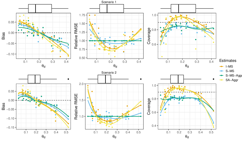
Figure 2: Ensamble distribution of biases, relative RMSEs (i.e. divided by RMSEs of S-MS-Aggr) and frequentist coverages with respect to the population poverty rate $\theta_{d}$.

From each synthetic population, $B=1,000$ samples are drawn following a two-stages sampling procedure with rates of approximately 2%. To account for the presence of out-of-sample sub-areas, each drawn sample does not include units from 37 sub-areas belonging to 15 areas. In this way, half of the areas include individuals from all the sub-areas, and, in the other half, units pertaining to two or three sub-areas are not observed.

		LOOIC	MAPE (%)			ARRMSE
Scen.	Estimates	Overall	No OOS	OOS	Overall	No OOS	OOS	Overall
1	I-MS	-17.3	33.7	45.5	39.6	0.378	0.440	0.409
	S-MS	-29.5	28.2	36.4	32.3	0.351	0.465	0.408
	S-MS-Aggr	-	25.8	36.2	31.0	0.323	0.468	0.395
	SA-Aggr	-	27.8	40.3	34.0	0.334	0.463	0.398
2	I-MS	-17.1	50.1	50.5	50.3	0.426	0.454	0.440
	S-MS	-33.5	30.5	36.9	33.7	0.386	0.472	0.429
	S-MS-Aggr	-	27.4	36.9	32.1	0.347	0.478	0.413
	SA-Aggr	-	31.6	39.4	35.5	0.386	0.473	0.429

Table 1: LOOIC, MAPE and ARRMSE for the area level. Concerning MAPE and ARRMSE, values obtained for the areas without missing sub-areas (No OOS), with missing sub-areas (OOS) and overall are distinctly reported.

The frequentist properties of the benchmarked estimators $\hat{\tilde{\theta}}_{dj}$ and $\hat{\tilde{\theta}}_{d}$ obtained under different models are compared: S-MS, SA and I-MS. Note that, with the suffix -Aggr we denote area-level estimates defined as in (3). Let us indicate with $\theta_{i}$ as the true value for the generic area or sub-area $i$ and $\hat{\tilde{\theta}}_{i}^{(b)}$ as the benchmarked estimate at iteration $b$. To determine the 90% credible intervals we consider 5^th and $95^{th}$ posterior percentiles, labeled as $\tilde{\theta}_{i,L}^{(b)}$ and $\tilde{\theta}_{i,U}^{(b)}$. We define bias, root mean squared error (RMSE) and coverage for 90% credible intervals for each area or sub-area as

$$\text{Bias}\left[\hat{\tilde{\theta}}_{i}\right]=\frac{1}{B}\sum_{b=1}^{B}\left(\hat{\tilde{\theta}}_{i}^{(b)}-\theta_{i}\right),\quad\text{RMSE}\left[\hat{\tilde{\theta}}_{i}\right]=\sqrt{\frac{1}{B}\sum_{b=1}^{B}\left(\hat{\tilde{\theta}}_{i}^{(b)}-\theta_{i}\right)^{2}},$$

$$\text{Cov}\left[\tilde{\theta}_{i}\right]=\frac{1}{B}\sum_{b=1}^{B}\bm{1}\left\{\theta_{i}\in\left[\tilde{\theta}_{i,L}^{(b)};\tilde{\theta}_{i,U}^{(b)}\right]\right\}.$$

As summary measures of bias and RMSE, we define the mean absolute percentage mean squared error (MAPE) and the average relative root mean squared error (ARRMSE) as

$$\text{MAPE (\%)}=\frac{100}{BI}\sum_{b=1}^{B}\sum_{i=1}^{I}\frac{\hat{\tilde{\theta}}_{i}^{(b)}-\theta_{i}}{\theta_{i}},\quad\text{ARRMSE}=\frac{1}{I}\sum_{i=1}^{I}\frac{\text{RMSE}\left[\hat{\tilde{\theta}}_{i}\right]}{\theta_{i}}.$$

Lastly, as a measure of the model goodness-of-fit, the leave-one-out information criterion (LOOIC, Vehtari et al., 2017) is considered.

Interesting cues about the performances of the compared area-specific estimators can be deduced from Figure 2. It reports the relative RMSEs, obtained by dividing each RMSE by the corresponding S-MS-Aggr RMSE, jointly with biases and frequentist coverages versus the population values. In both scenarios, the S-MS-Aggr estimators are characterized by lower biases, if compared to I-MS and SA cases: such differences become relevant for areas whose true values are far from their average (about 50% of them). Such a decrease in the bias leads to some differences also in the behaviour of RMSE too: S-MS-Aggr produces more efficient estimators in the tails of the ensamble distribution of population poverty rates $\{\theta_{1},\dots,\theta_{D}\}$, becoming less efficient in the central part of the distribution. By focusing on the 90% credible intervals, we observe that S-MS-Aggr is affected by a slight under-coverage (median: 0.83 in scenario 1 and 0.81 in scenario 2). However, the performances deteriorate more slowly if compared to the other methods in the non-central parts of the ensamble distribution. Table 1 summarises the overall performances of the methods across areas. The MAPE points out the ability of S-MS-Aggr in reducing the bias, registering lower values both in areas with and without out-of-sample sub-areas; conversely, ARRMSE highlights that the average performances are quite similar.

We can point out that the I-MS model, characterized by the absence of an area-specific random effect, leads to poorer performances if compared to all the other strategies. This is more evident in Scenario 2 where the data-generating process mimics the case $\sigma_{a}>\sigma_{s}$. Targeting the estimation of sub-area parameters, summaries reported in Table S1 of the Supplementary Material point out that the three models behave quite similarly, with the exception of I-MS, which still shows lower performances in Scenario 2. Lastly, we highlight that the average LOOIC of the S-MS model is widely lower both for sub-area (Table S1) and area (Table 1) levels in both scenarios, denoting a remarkable improvement in the predictive abilities of this model.

In summary, the estimators under the S-MS model have more stable performances along the support. They are characterized by a more moderate shrinkage and, for this reason, they perform better on the tails of the poverty rates ensemble distribution, and slightly better than their competitors on average. Small and, especially, large poverty rates are relevant for the implementation of geographically targeted alleviation policies as they can identify poverty hotspots. Therefore, an improvement in the estimation of such values may be of great importance in this context.

6 Poverty mapping in Bangladesh

The aim of this section is to map poverty in Bangladesh at multiple levels of administrative divisions: the Administrative Level AL-2, comprising $D=64$ zilas as areas, and the AL-3 with $M=544$ upazilas as sub-areas. The target poverty measure is the proportion of people below the 20th percentile of the WI national distribution. We consider DHS survey data complemented with RS and geographical data available from multiple open sources. Data and sources are shortly illustrated in Section 6.1, whereas results are discussed in Section 6.2.

6.1 Data

The Bangladesh DHS, of which we consider the 2014 wave, targets the population residing in non-institutional dwelling units by providing a two-stage stratified sample with 17,300 households and $n=81,624$ individuals overall. The sample sizes in terms of individuals range from 135 to 4,730 (median 986) for zilas and from 16 to 1,884 (median: 160) for upazilas. All the zilas are in-sample, whereas about one third of upazilas (179) are not included in the sample.

For each household, a WI score is computed by combining a set of answers on the availability of durable assets and housing welfare characteristics (Fabic et al., 2012). Households laying in the first quintile of the national distribution of WI are labeled as poor. Since poverty is usually investigated individually, the analysis is carried out at the individual level by assuming that all components of the same household share the same WI score. A sampling weight is associated to each household, accounting for unequal probabilities of selection and non-responses. The survey estimates, as defined in Section 2, range from 0 to 0.53 (median: 0.21) with just one 0 value for zilas; while they span from 0 to 0.96 (median: 0.16) with 66 zero values for upazilas.

To retrieve the effective sample sizes, we opt to estimate the design effect starting from the strata level as in Schmid et al. (2017). Such uncertainty estimates confirm the unreliability of survey estimates both at zila and upazila levels motivating us to employ SAE: we observe coefficients of variation higher than 0.20 in more than 80% of overall in-sample estimates. We note that effective sample sizes are much lower than the effective ones because the poverty status is defined at the household level and the correlation within clusters (i.e. Census enumeration areas) is very strong.

	LOOIC (Standard Error)
Models	SA	I-MS	S-MS
Zila level	-      (-)	-137.9 (12.5)	-150.9 (10.9)
Upazila level	-101.8 (30.4)	-98.4 (31.2)	-115.9 (29.5)

Table 2: LOOIC values and their standard errors for all the considered models.

We integrate $46$ RS variables as covariates computed both at the area and sub-area levels by cutting rasters through shapefiles (for more details, see De Nicolò et al., 2022, and Section S4 in the Supplementary Material). Specifically, we consider the demographic composition of areas and sub-areas by including the population density and its disaggregation by age and sex classes. The nighttime light radiance and the distances to main facilities and infrastructures (e.g. nearest city or healthcare site) are included as indicators of area urbanization and economic development. As the agricultural sector is a driving force for Bangladeshi economy, its territorial and climatic characterization may be proxies of productivity. The first one has been considered by including land-use variables that specify the distance from nearest areas with specific use classification (e.g. cultivated, woody-tree, artificial surface), the elevation above sea level and topographic slope. The second one is fulfilled through bio-climatic variables such as the overall and seasonal variations of temperature and rainfall (e.g., annual mean, standard deviation and temperature diurnal range).

6.2 Results

The alternative models SA, I-MS and S-MS are fitted on Bangladeshi data. Table 2 provides details about the model comparison in terms of LOOIC, for both spatial levels. According to it, the S-MS model shows better goodness-of-fit with respect to the other proposals, while SA and I-MS perform similarly. The main motivation for this finding is that the S-MS model has the area-specific random effect $u_{d}$, $\forall d$, characterizing the distributions at both levels, thus promoting an exchange of information between areas and sub-areas. Conversely, the other models define $u_{d}$ at only one level, thereby being informed only by observations at the corresponding level. This translates into a better ability of S-MS model to capture specific area features through random effects. To elaborate more on this point, the ensemble distributions of $\mathbb{E}[u_{d}|\mathbf{y}]$ are depicted in the left panel of Figure 3: note that under SA and I-MS models such distributions are markedly more concentrated around zero, not capturing area-specific peculiarities. Looking at the ensemble distribution of $\mathbb{E}[v_{dj}|\mathbf{y}]$, shown in the right panel of Figure 3, we observe that upazila effects seem partially absorbed by zila effects for the S-MS model. However, no relevant differences among models are recorded in this case.

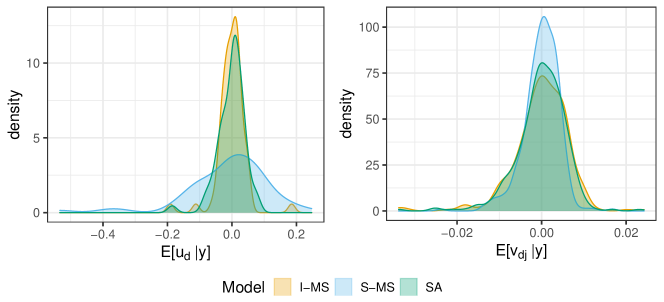
Figure 3: Densities of posterior means of $u_{d}$ and $v_{dj}$, $\forall d$, $\forall j$, for each model.

To simplify discussion, from now on, we focus on S-MS model estimates due to the aforementioned reasons. To obtain benchmarked estimates with respect to the national level, we project the posterior distributions of $\theta_{dj}$, $\forall d$, $\forall j$ exploiting the result of Theorem 1. Exploiting the definition of the response, we set $t=0.2$. We compare the original posterior distributions with their projections under the proposed Bregman and weighted squared error loss functions. In particular, Figure 4 shows it for two upazilas with poverty rates close to zero. Note that, under the weighted squared error loss, projections can be markedly outside the support taking negative values. In contrast, under the Bregman loss function, benchmarked posteriors are correctly defined in $(0,1)$.

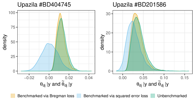
Figure 4: Posterior distributions of benchmarked and unbenchmarked estimates in two upazilas.

The shrinking process induced by the model at both spatial levels is depicted in Figure 5, by comparing survey estimates with model-based estimates. As expected, the shrinkage is stronger at the upazila level, given the downward precision of survey estimates. The differences between survey and model-based estimates may be high in case of very low effective sample sizes. Moreover, the right panel of Figure 5 shows that discrepancies at the area level may be also due to a high percentage of out-of-sample sub-areas. In Figure 6, ensemble densities of sub-area estimates split up between in-sample and out-of-sample ones, together with a collection of the most relevant covariates. This illustrates that the composition of out-of-sample sub-areas is quite heterogeneous, incorporating both remote sub-areas (e.g. a large number of sub-areas on Chittagong Hill tracts) and urban or suburban ones. As a consequence, the out-of-sample poverty rates show a higher polarization between a set of urban and less poor sub-areas and a set of very poor rural ones. The latter is characterized by greater poverty levels than those fitted for in-sample sub-areas. This confirms that the sample selection process determining out-of-sample sub-areas can be affected by specific features.

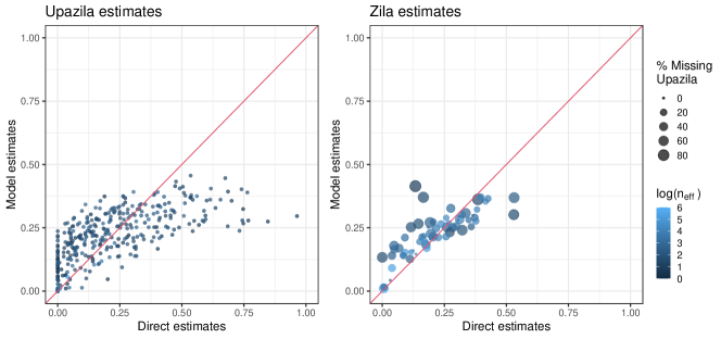
Figure 5: Shrinkage process at both spatial levels, bisector line in red.

The spatial distribution of model-based estimates is displayed in Figure 7, enabling us to highlight the heterogeneity of poverty rates inside each zila. This is not clear by the zila map that averages out such estimates; whereas, at a finer level, the upazila map bears additional and valuable information. The reduction of standard deviation of model-based estimates with respect to survey-based ones is of $51\%$ on average for zilas and $77\%$ for upazilas.

At a first glance, the poverty patterns are consistent with the literature (Kam et al., 2005; Imam et al., 2019), capturing consolidated dynamics. The metropolitan regions of Dhaka and Chittagong retain the lowest poverty levels, in contrast with peripheral areas. High poverty incidence domains overlap with ecologically poor zones (Kam et al., 2005). We can mention the territories more severely exposed to climate change effects and floodings such as the Haor depression (Sylhet basin lowlands) in the north-east, some areas at the edge of major rivers (Haque and Jahan, 2015), those exposed to droughts in the Rangpur division (north-west) and the Chittagong Hill Tract (south-east). On the other hand, the drought-prone southern Rajshahi and Khulna divisions experience lower poverty levels due to the good irrigation coverage (Kam et al., 2005). However, when disaggregating estimates at the upazila level, the picture becomes more clear. The poorest regions present a remarkable variety and it is possible to detect few upazilas having lower poverty levels than the neighbour ones. They correspond to main urban centers (indicated by red dots in Figure 7) such as Rangpur, Dinajpur, and Saidpur cities in Rangpur division; Sylhet, Kishoreganj, and Mymensingh in the north-east side and Raozan in the south-east side.

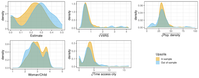
Figure 6: Densities of model-based estimates and the most relevant covariates compared between in-sample and out-of-sample sub-areas.

7 Conclusions

In this paper, we introduce a multi-scale modeling framework for poverty mapping at multiple spatial resolutions to avoid the scaling problem. The main aim is to produce reliable poverty maps that are coherent at different geographical layers. Such tools are valuable for poverty evaluation, poverty targeting and to develop place-based policies. On this line, we complement the proposal with a novel benchmarking algorithm that ensures the accordance of poverty estimates across levels. This allows to preserve poverty rate estimates and associated credible intervals within their support, restricted to $(0,1)$.

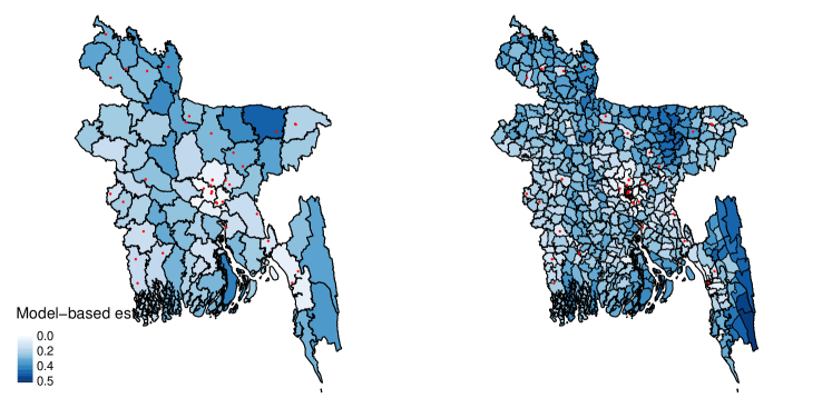
Figure 7: Model-based estimates at the zila level (left-hand side) and at the upazila level (right-hand side); red points indicate the 37 major cities.

The simulation study we carried out highlights the effectiveness of our proposal, showing better performances with respect to existing alternatives. In particular, this is evident for poverty rates laying in the tails of their distribution, which are less shrunken towards the average. In this way, our modeling strategy is able to retain domains with extremely high poverty rates: this has relevant practical implications since poverty hotspots need to be identified as being the target of poverty relief actions. In our application on Bangladeshi data, rural and remote regions that mostly overlap with droughts- and floods-prone zones with high exposure to climate change effects, are classified as very poor. In this sense, geo-targeted policies may foster risk mitigation strategies (e.g., insurance) as well as further expand irrigation coverages via specific water management policies (Pal et al., 2011; Hossain et al., 2022). Furthermore, our multi-scale poverty mapping approach permits us to spot critical zones located within larger administrative units.

It is possible to extend our proposal to explicitly account for the spatial structure in the statistical model, similarly to Aregay et al. (2016). However, results of our application do not provide evidence of a residual spatial trend. This can be due to the spatial informative power of remote sensing covariates employed in the model. Another future extension consists in considering also other quintiles of the WI index national distribution through a multivariate framework. Moreover, moving beyond poverty measurement, our proposal may be applied to map other well-being measures such as inequality indicators.

References

- Aitchison (1992) J. Aitchison. On criteria for measures of compositional difference. Mathematical Geology, 24(4):365–379, 1992.
- Allard and Allard (2017) S. W. Allard and S. Allard. Places in need: The changing geography of poverty. Russell Sage Foundation, 2017.
- Aregay et al. (2016) M. Aregay, A. B. Lawson, C. Faes, R. S. Kirby, R. Carroll, and K. Watjou. Multiscale measurement error models for aggregated small area health data. Statistical methods in medical research, 25(4):1201–1223, 2016.
- Aregay et al. (2017) M. Aregay, A. B. Lawson, C. Faes, R. S. Kirby, R. Carroll, and K. Watjou. Comparing multilevel and multiscale convolution models for small area aggregated health data. Spatial and Spatio-temporal Epidemiology, 22:39–49, 2017.
- Banerjee et al. (2005) A. Banerjee, X. Guo, and H. Wang. On the optimality of conditional expectation as a bregman predictor. IEEE Transactions on Information Theory, 51(7):2664–2669, 2005.
- Bell et al. (2013) W. R. Bell, G. S. Datta, and M. Ghosh. Benchmarking small area estimators. Biometrika, 100(1):189–202, 2013.
- Benedetti et al. (2022) M. H. Benedetti, V. J. Berrocal, and R. J. Little. Accounting for survey design in bayesian disaggregation of survey-based areal estimates of proportions: An application to the american community survey. The Annals of Applied Statistics, 16(4):2201–2230, 2022.
- Bigman and Fofack (2000) D. Bigman and H. Fofack. Geographical targeting for poverty alleviation: An introduction to the special issue. The World Bank Economic Review, 14(1):129–145, 2000.
- Bikauskaite et al. (2022) A. Bikauskaite, I. Molina, and D. Morales. Multivariate mixture model for small area estimation of poverty indicators. Journal of the Royal Statistical Society Series A: Statistics in Society, 185(Supplement_2):S724–S755, 2022.
- Carpenter et al. (2017) B. Carpenter, A. Gelman, M. D. Hoffman, D. Lee, B. Goodrich, M. Betancourt, M. Brubaker, J. Guo, P. Li, and A. Riddell. Stan: A probabilistic programming language. Journal of statistical software, 76(1), 2017.
- Casas-Cordero Valencia et al. (2016) C. Casas-Cordero Valencia, J. Encina, and P. Lahiri. Poverty mapping for the chilean comunas. Analysis of Poverty Data by Small Area Estimation, pages 379–404, 2016.
- Christiaensen and Todo (2014) L. Christiaensen and Y. Todo. Poverty reduction during the rural–urban transformation–the role of the missing middle. World Development, 63:43–58, 2014.
- Corral et al. (2022) P. Corral, I. Molina, A. Cojocaru, and S. Segovia. Guidelines to small area estimation for poverty mapping. 2022.
- Datta et al. (2011) G. Datta, M. Ghosh, R. Steorts, and J. Maples. Bayesian benchmarking with applications to small area estimation. Test, 20(3):574–588, 2011.
- De Nicolò et al. (2022) S. De Nicolò, E. Fabrizi, and A. Gardini. Extended beta models for poverty mapping. an application integrating survey and remote sensing data in Bangladesh. In Quaderni di Dipartimento. Serie Ricerche. 2022.
- Dunson and Neelon (2003) D. B. Dunson and B. Neelon. Bayesian inference on order-constrained parameters in generalized linear models. Biometrics, 59(2):286–295, 2003.
- Elbers et al. (2007) C. Elbers, T. Fujii, P. Lanjouw, B. Özler, and W. Yin. Poverty alleviation through geographic targeting: How much does disaggregation help? Journal of Development Economics, 83(1):198–213, 2007.
- Erciulescu et al. (2019) A. L. Erciulescu, N. B. Cruze, and B. Nandram. Model-based county level crop estimates incorporating auxiliary sources of information. Journal of the Royal Statistical Society: Series A (Statistics in Society), (1):283–303, 2019.
- Fabic et al. (2012) M. S. Fabic, Y. Choi, and S. Bird. A systematic review of demographic and health surveys: data availability and utilization for research. Bulletin of the World Health Organization, 90:604–612, 2012.
- Fabrizi et al. (2016a) E. Fabrizi, M. Ferrante, and C. Trivisano. Hierarchical beta regression models for the estimation of poverty and inequality parameters in small areas. Analysis of Poverty Data by Small Area Methods. John Wiley and Sons, pages 299–314, 2016a.
- Fabrizi et al. (2016b) E. Fabrizi, M. R. Ferrante, and C. Trivisano. Bayesian beta regression models for the estimation of poverty and inequality parameters in small areas. Analysis of poverty data by small area estimation, pages 299–314, 2016b.
- Fan and Cho (2021) S.-g. Fan and E. E. Cho. Paths out of poverty: International experience. Journal of Integrative Agriculture, 20(4):857–867, 2021.
- Ferrari and Cribari-Neto (2004) S. Ferrari and F. Cribari-Neto. Beta regression for modelling rates and proportions. Journal of Applied Statistics, 31(7):799–815, 2004.
- Galasso and Ravallion (2005) E. Galasso and M. Ravallion. Decentralized targeting of an antipoverty program. Journal of Public economics, 89(4):705–727, 2005.
- Gauci (2005) A. Gauci. Spatial maps. targeting & mapping poverty. London: United Nations. Economic Commission for Africa, 2005.
- Ghosh et al. (2015) M. Ghosh, T. Kubokawa, and Y. Kawakubo. Benchmarked empirical bayes methods in multiplicative area-level models with risk evaluation. Biometrika, 102(3):647–659, 2015.
- Hájek (1971) J. Hájek. Discussion of ‘an essay on the logical foundations of survey sampling, part i’, by d. basu. Foundations of Statistical Inference, page 326, 1971.
- Hall et al. (2023) O. Hall, F. Dompae, I. Wahab, and F. M. Dzanku. A review of machine learning and satellite imagery for poverty prediction: Implications for development research and applications. Journal of International Development, 2023.
- Haque and Jahan (2015) A. Haque and S. Jahan. Impact of flood disasters in bangladesh: A multi-sector regional analysis. International Journal of Disaster Risk Reduction, 13:266–275, 2015.
- Hossain et al. (2022) M. S. Hossain, G. M. Alam, S. Fahad, T. Sarker, M. Moniruzzaman, and M. G. Rabbany. Smallholder farmers’ willingness to pay for flood insurance as climate change adaptation strategy in northern bangladesh. Journal of Cleaner Production, 338:130584, 2022.
- Imam et al. (2019) M. F. Imam, M. A. Islam, M. A. Alam, M. J. Hossain, and S. Das. Small area estimation of poverty in rural bangladesh. The Bangladesh Journal of Agricultural Economics, 40(1&2):1–16, 2019.
- Janicki (2020) R. Janicki. Properties of the beta regression model for small area estimation of proportions and application to estimation of poverty rates. Communications in Statistics-Theory and Methods, 49(9):2264–2284, 2020.
- Janicki and Vesper (2017) R. Janicki and A. Vesper. Benchmarking techniques for reconciling bayesian small area models at distinct geographic levels. Statistical Methods & Applications, 26(4):557–581, 2017.
- Jean et al. (2016) N. Jean, M. Burke, M. Xie, W. M. Davis, D. B. Lobell, and S. Ermon. Combining satellite imagery and machine learning to predict poverty. Science, 353(6301):790–794, 2016.
- Kam et al. (2005) S.-P. Kam, M. Hossain, M. L. Bose, and L. S. Villano. Spatial patterns of rural poverty and their relationship with welfare-influencing factors in bangladesh. Food Policy, 30(5-6):551–567, 2005.
- Kolaczyk and Huang (2001) E. D. Kolaczyk and H. Huang. Multiscale statistical models for hierarchical spatial aggregation. Geographical Analysis, 33(2):95–118, 2001.
- Kraay and McKenzie (2014) A. Kraay and D. McKenzie. Do poverty traps exist? assessing the evidence. Journal of Economic Perspectives, 28(3):127–148, 2014.
- Liu et al. (2014) B. Liu, P. Lahiri, and G. Kalton. Hierarchical bayes modeling of survey-weighted small area proportions. Survey Methodology, 40(1):1–14, 2014.
- Liu et al. (2017) Y. Liu, J. Liu, and Y. Zhou. Spatio-temporal patterns of rural poverty in china and targeted poverty alleviation strategies. Journal of rural studies, 52:66–75, 2017.
- Louie and Kolaczyk (2006) M. M. Louie and E. D. Kolaczyk. A multiscale method for disease mapping in spatial epidemiology. Statistics in medicine, 25(8):1287–1306, 2006.
- Molina et al. (2014) I. Molina, B. Nandram, and J. Rao. Small area estimation of general parameters with application to poverty indicators: A hierarchical bayes approach. The Annals of Applied Statistics, 8(2):852–885, 2014.
- Okonek and Wakefield (2022) T. Okonek and J. Wakefield. A computationally efficient approach to fully bayesian benchmarking. arXiv preprint arXiv:2203.12195, 2022.
- Pal et al. (2011) S. K. Pal, A. J. Adeloye, M. S. Babel, and A. Das Gupta. Evaluation of the effectiveness of water management policies in bangladesh. Water Resources Development, 27(02):401–417, 2011.
- Patra (2019) S. Patra. Constrained Bayesian inference through posterior projection with applications. PhD thesis, 2019.
- Piironen and Vehtari (2017) J. Piironen and A. Vehtari. Sparsity information and regularization in the horseshoe and other shrinkage priors. Electronic Journal of Statistics, 11(2):5018 – 5051, 2017. doi: 10.1214/17-EJS1337SI.
- Pirani (2014) E. Pirani. Wealth index. Encyclopedia of Quality of Life and Well-Being Research. Springer, Dordrecht. https://doi. org/10.1007/978-94-007-0753-5_3202, 2014.
- Poirier et al. (2020) M. J. Poirier, K. A. Grépin, and M. Grignon. Approaches and alternatives to the wealth index to measure socioeconomic status using survey data: a critical interpretive synthesis. Social Indicators Research, 148(1):1–46, 2020.
- Pratesi and Salvati (2016) M. Pratesi and N. Salvati. Introduction on measuring poverty at local level using small area estimation methods. In Analysis of poverty data by small area estimation, chapter 1, pages 1–18. Wiley Online Library, 2016.
- Puurbalanta (2021) R. Puurbalanta. A clipped gaussian geo-classification model for poverty mapping. Journal of Applied Statistics, 48(10):1882–1895, 2021.
- Rao and Molina (2015) J. N. Rao and I. Molina. Small area estimation. John Wiley & Sons, 2015.
- Schmid et al. (2017) T. Schmid, F. Bruckschen, N. Salvati, and T. Zbiranski. Constructing sociodemographic indicators for national statistical institutes by using mobile phone data: estimating literacy rates in senegal. Journal of the Royal Statistical Society: Series A (Statistics in Society), 180(4):1163–1190, 2017.
- Sen et al. (2018) D. Sen, S. Patra, and D. Dunson. Constrained inference through posterior projections. arXiv preprint arXiv:1812.05741, 2018.
- Sohnesen et al. (2022) T. P. Sohnesen, P. Fisker, and D. Malmgren-Hansen. Using satellite data to guide urban poverty reduction. Review of Income and Wealth, 68:S282–S294, 2022.
- Steele et al. (2017) J. E. Steele, P. R. Sundsøy, C. Pezzulo, V. A. Alegana, T. J. Bird, J. Blumenstock, J. Bjelland, K. Engø-Monsen, Y.-A. De Montjoye, A. M. Iqbal, et al. Mapping poverty using mobile phone and satellite data. Journal of The Royal Society Interface, 14(127):20160690, 2017.
- Torabi and Rao (2014) M. Torabi and J. Rao. On small area estimation under a sub-area level model. Journal of Multivariate Analysis, 127:36–55, 2014.
- Tzavidis et al. (2018) N. Tzavidis, L.-C. Zhang, A. Luna, T. Schmid, N. Rojas-Perilla, l. R. Gordon, P. Williamson, T. King, M. G. Ranalli, P. A. Smith, et al. From start to finish. Journal of the Royal Statistical Society. Series A (Statistics in Society), 181(4):927–979, 2018.
- Vehtari et al. (2017) A. Vehtari, A. Gelman, and J. Gabry. Practical bayesian model evaluation using leave-one-out cross-validation and waic. Statistics and Computing, 27(5):1413–1432, 2017.
- Zhang and Bryant (2020) J. L. Zhang and J. Bryant. Fully bayesian benchmarking of small area estimation models. Journal of official statistics, 36(1):197–223, 2020.
- Zhao et al. (2019) X. Zhao, B. Yu, Y. Liu, Z. Chen, Q. Li, C. Wang, and J. Wu. Estimation of poverty using random forest regression with multi-source data: A case study in bangladesh. Remote Sensing, 11(4):375, 2019.
- Zhou and Liu (2022) Y. Zhou and Y. Liu. The geography of poverty: Review and research prospects. Journal of Rural Studies, 93:408–416, 2022.