High order entropy stable discontinuous Galerkin spectral element methods through subcell limiting

Abstract

Subcell limiting strategies for discontinuous Galerkin spectral element methods do not provably satisfy a semi-discrete cell entropy inequality. In this work, we introduce an extension to the subcell and monolithic convex limiting strategies [1, 2, 3] that satisfies the semi-discrete cell entropy inequality by formulating the limiting factors as solutions to an optimization problem. The optimization problem is efficiently solved using a deterministic greedy algorithm. We also discuss the extension of the proposed subcell limiting strategy to preserve general convex constraints. Numerical experiments confirm that the proposed limiting strategy preserves high-order accuracy for smooth solutions and satisfies the cell entropy inequality.

1 Introduction

In computational fluid dynamics simulations, higher resolutions are increasingly necessary for a wide range of applications [4]. In certain scenarios, high-order accurate numerical methods are preferred over low-order methods due to their improved accuracy per degree of freedom, and comparable efficiency [5]. High-order discontinuous Galerkin (DG) methods are notably well-suited for handling convection-dominated problems and yield simple and efficient implementations due to the inherent locality of many operations [6]. Among DG methods, the DG spectral element method (DGSEM) is one of the most computationally efficient high-order discretization techniques, due to the tensor-product structure of the associated operators.

Unfortunately, high-order DGSEM often encounter stability issues when solving nonlinear hyperbolic conservation laws. These issues arise due to the loss of nonlinear stability and ill-defined physical quantities such as negative density and pressure in compressible flows. Traditional stabilization techniques, such as filtering and artificial viscosity [7, 8] are commonly employed in combination with DGSEM. However, most of these methods require heuristic tuning of parameters and lack provable robustness and high-order convergence for smooth solutions.

For high-order DG schemes, Zhang, Shu, and their colleagues introduced simple, effective, and high-order accuracy preserving scaling limiters for systems of conservation laws [9, 10, 11]. The core idea is to utilize a strong stability preserving Runge-Kutta (SSPRK) time integrator to compute the average of the DG solution on each element, which satisfies desired properties under a timestep condition. The limited solution is then constructed by scaling the high-order DG towards the DG average.

Another popular class of limiting strategies is flux-corrected transport (FCT) algorithms [12, 13]. Inspired by FCT, Kuzmin designed algebraic flux correction (AFC) schemes, which provide a general framework for designing multidimensional flux limiters [14]. AFC schemes introduce a novel artificial diffusion operator and a conservative flux decomposition to generalize the limiting technique of FCT algorithms. The underlying low-order method is a generalization of the local Lax-Friedrichs (LLF) method to nodal finite element discretizations [14, 15]. A subcell limiting strategy is then proposed to allow the limiting factors to vary within an element in the context of high-order Bernstein finite element [16]. Pazner later extended this subcell limiting strategy to the DGSEM in a dimension-by-dimension fashion [1].

In the context of subcell limiting, there are two major approaches to ensure some types of entropy inequality. One approach involves enforcing a discrete minimum principle on specific entropy [1, 2]. However, this approach is limited to compressible flows and may reduce the accuracy of the solution to at most second order for smooth solutions. Another recent approach is to enforce Tadmor’s entropy condition on subcell algebraic fluxes [17, 3]. This approach also does not preserve high-order accuracy for DGSEM.

This work aims to address the loss of high-order accuracy near smooth regions when applying subcell limiter-based entropy stabilization. The main motivation comes from high-order entropy stable Discontinuous Galerkin (ESDG) discretizations and other schemes, where a semi-discrete cell entropy balance is satisfied [18, 19, 20, 21, 22, 23, 24, 25, 26]. In contrast, the aforementioned entropy stabilization techniques enforce an entropy stability inequality at the nodal level. The essential idea of the proposed limiting strategy is to enforce the cell entropy balance through the subcell limiting strategy, which can be formulated as a linear program over each element. This linear program can be solved efficiently and optimally with a simple greedy algorithm. Furthermore, the proposed entropy stabilization can be easily extended to preserve more general convex constraints.

The outline of the paper is as follows: Section 2 gives a brief overview of the nonlinear conservation laws, the notations used in the paper, and some background knowledge on DGSEM. Section 3 presents the semi-discrete entropy stable subcell limiting technique. In Section 4, we provide various numerical experiments in 1D and 2D to verify the high-order convergence, entropy stability, and robustness of the proposed limiting strategy. Finally, we summarize our work in Section 5.

2 Background knowledge

In this work, we focus on solving the nonlinear hyperbolic conservation laws in two space-dimensions, with the understanding that the theoretical findings presented in this paper can be readily applied to three-dimensional settings.

2.1 On notation

We adopt the notation convention introduced in [20]. Lower and upper case bold fonts (for example, $\bm{A}$ and $\bm{u}$) refer to vector and matrix quantities, respectively. Spatially discrete quantities are written in bold sans serif font (e.g., $\bm{\mathsf{x}}$). To ensure clarity, continuous real functions evaluated over spatially discrete quantities are interpreted as point-wise evaluations. For instance,

$$\bm{\mathsf{x}}=\begin{bmatrix}\bm{x}_{1}\\ \vdots\\ \bm{x}_{n}\end{bmatrix},\qquad u:\mathbb{R}\rightarrow\mathbb{R},\qquad u(\bm{\mathsf{x}})=\begin{bmatrix}u(\bm{x}_{1})\\ \vdots\\ u(\bm{x}_{n})\end{bmatrix}$$

We note that we abuse notation and adopt the convention that $\bm{\mathsf{A}}\bm{\mathsf{u}}$ represents the Kronecker product $(\bm{\mathsf{A}}\otimes\bm{\mathsf{I}}_{N^{c}})\bm{\mathsf{u}}$ [24], where operator $\bm{\mathsf{A}}$ is applied to each scalar component $\bm{\mathsf{u}}$. We will use either a number subscript $\bm{\mathsf{A}}_{1},\bm{\mathsf{A}}_{2}$, or a letter subscript $\bm{\mathsf{A}}_{r}$,$\bm{\mathsf{A}}_{s}$ interchangeably to indicate the coordinates of discrete operators. For the sake of notational clarity, this work will present the theory on the reference element $\widehat{D}$ and will ignore the geometric terms involved. For more information on how the proposed framework can be applied to mapped elements and curved meshes, readers can look into Appendix A of our recent manuscript [27].

For DG discretizations, let $u(\bm{x})$ be a scalar function on an element $D$. We define $u$ as its “interior” and $u^{+}$ as its “exterior” values across the face shared by neighbor $D^{+}$.

2.2 Nonlinear conservation laws

A $d$-dimensional nonlinear hyperbolic conservation law with $N_{c}$ components is given by:

$$\frac{\partial\bm{u}}{\partial t}+\nabla\cdot\bm{f}\left(\bm{u}\right)=0,\qquad\bm{u}\in\mathbb{R}^{N_{c}},\qquad\bm{f}_{i}\left(\bm{u}\right):\mathbb{R}^{N_{c}}\rightarrow\mathbb{R}^{N_{c}},\quad i=1,\dots,d.$$ (1)

In particular, we are interested in systems with an associated convex mathematical entropy $\eta\left(\bm{u}\right)$, whose physically relevant solutions (defined as the limit solutions for an appropriately defined vanishing viscosity) satisfy an entropy inequality:

$$\frac{\partial\eta\left(\bm{u}\right)}{\partial t}+\nabla\cdot\bm{F}\left(\bm{u}\right)\leq 0,$$ (2)

where $\bm{F}\left(\bm{u}\right)$ is referred to as the entropy flux satisfying the following identity:

$$\left(\nabla_{\bm{u}}\bm{F}\left(\bm{u}\right)\right)^{T}=\bm{v}^{T}\nabla_{\bm{u}}\bm{f}\left(\bm{u}\right),\qquad\bm{v}=\nabla_{\bm{u}}\eta\left(\bm{u}\right).$$ (3)

$\bm{v}$ is referred to as the entropy variables. A cell entropy balance is obtained by integrating the entropy inequality (2) over a domain $D$ and applying integration by parts and chain rule:

$$\int_{D}\frac{\partial\eta\left(\bm{u}\right)}{\partial t}+\int_{\partial D}\bm{v}^{T}\bm{f}\left(\bm{u}\left(\bm{v}\right)\right)-\bm{\psi}\left(\bm{v}\right)\leq 0,$$ (4)

where $\bm{\psi}(\bm{v})=\bm{v}^{T}\bm{f}(\bm{u}\left(\bm{v}\right))-F(\bm{u}\left(\bm{v}\right))$ is referred to as the entropy potential.

2.3 Discretizations

The subcell limiting strategy is based on blending a high-order accurate discretization and a low-order structure-preserving discretization constructed using algebraic viscosity. In this section, we will provide a brief introduction to the two types of discretizations that form the basis of the proposed limiting strategy. We will restrict ourselves to 2D for simplicity of presentations, but the idea is straightforward to extend to 3D. For both discretizations, the domain $\Omega$ is decomposed into non-overlapping quadrilateral elements $D^{k}$, each of which is the image of a reference element $\hat{D}$ under an invertible mapping $\bm{\Phi}^{k}$. The reference approximation basis of degree $N$ is defined as the Lagrange basis on Legendre-Gauss-Lobatto (LGL) quadrature nodes $\left\{r_{i}\right\}_{i=1}^{N+1}$:

$$\phi_{i,j}\left(r,s\right)={\color[rgb]{0,0,0}{L_{i}}}\left(r\right){\color[rgb]{0,0,0}{L_{i}}}\left(s\right),\qquad{\color[rgb]{0,0,0}{L_{i}}}\left(r\right)=\prod\limits_{j\neq i}\frac{r-r_{i}}{r_{j}-r_{i}}.$$ (5)

In this work, we concentrate on Cartesian grids for the sake of simplicity. The extension to curvilinear meshes is discussed in [1] and [27].

2.3.1 Discontinuous Galerkin spectral element discretization

The DGSEM discretization refers to DG discretizations whose underlying approximation basis is the Lagrange basis on LGL nodes and lumped mass matrix is defined with LGL quadrature weights. Since the quadrature nodes collocate with the interpolation nodes, the mass, differentiation, weighted differentiation, boundary integration, and face extrapolation matrices are defined as

$$\bm{\mathsf{M}}_{\rm 1D} =\begin{bmatrix}w_{1}&&\\ &\ddots&\\ &&w_{N+1}\end{bmatrix},\qquad\left(\bm{\mathsf{D}}_{\rm 1D}\right)_{ij}=\left.\frac{{\rm d}{\color[rgb]{0,0,0}{L_{j}}}}{{\rm d}{{r}}}\right|_{r=r_{j}},\qquad\bm{\mathsf{Q}}_{\rm 1D}=\bm{\mathsf{M}}_{\rm 1D}\bm{\mathsf{D}}_{\rm 1D}$$ (6)

$$\bm{\mathsf{B}}_{\rm 1D} =\begin{bmatrix}-1&0&\cdots&0&0\\ 0&0&\cdots&0&1\end{bmatrix},\qquad\bm{\mathsf{E}}_{\rm 1D}=\begin{bmatrix}1&0&\cdots&0&0\\ 0&0&\cdots&0&1\end{bmatrix},$$ (7)

where $\left\{w_{i}\right\}_{i=1}^{N+1}$ are the LGL quadrature weights.

Multidimensional operators are defined based on the tensor product structure of the reference approximation basis as follows

$$\bm{\mathsf{M}} =\bm{\mathsf{M}}_{\rm 1D}\otimes\bm{\mathsf{M}}_{\rm 1D},\qquad\bm{\mathsf{E}}=\bm{\mathsf{I}}_{N+1}\otimes\bm{\mathsf{E}}_{\rm 1D}$$ (8)

$$\bm{\mathsf{Q}}_{r} =\bm{\mathsf{M}}_{\rm 1D}\otimes\bm{\mathsf{Q}}_{\rm 1D},\qquad\bm{\mathsf{Q}}_{s}=\bm{\mathsf{Q}}_{\rm 1D}\otimes\bm{\mathsf{M}}_{\rm 1D},$$ (9)

$$\bm{\mathsf{B}}_{r} =\bm{\mathsf{M}}_{\rm 1D}\otimes\bm{\mathsf{B}}_{\rm 1D},\qquad\bm{\mathsf{B}}_{s}=\bm{\mathsf{B}}_{\rm 1D}\otimes\bm{\mathsf{M}}_{\rm 1D}.$$ (10)

Since the mass matrix $\bm{\mathsf{M}}$ is diagonal, we define $\bm{\mathsf{m}}_{i}=\bm{\mathsf{M}}_{ii}$ for simplicity of notation.

We can then write the discontinuous Galerkin spectral element discretization on the reference element as:

$$\bm{\mathsf{M}}\frac{{\rm d}\bm{\mathsf{u}}}{{\rm d}{{t}}}+\sum\limits_{k=1}^{2}\bm{\mathsf{Q}}_{k}\bm{\mathsf{f}}_{k}+\bm{\mathsf{E}}^{T}\bm{\mathsf{B}}_{k}\left(\bm{\mathsf{f}}_{k}^{*}\left(\bm{\mathsf{u}}_{f},\bm{\mathsf{u}}_{f}^{+}\right)-\bm{f}_{k}\left(\bm{\mathsf{u}}_{f}\right)\right)=0,$$ (11)

$$\bm{\mathsf{f}}_{k}=\bm{f}_{k}\left(\bm{\mathsf{u}}\right),\qquad\bm{\mathsf{u}}_{f}=\bm{\mathsf{E}}\bm{\mathsf{u}},$$

where $\bm{\mathsf{u}}_{f}^{+}$ denotes the interface value at the neighboring element interface. Readers can refer to Chapter 6 of [6] for its extention to multiple elements.

2.3.2 Low order semi-discrete entropy stable and positivity-preserving discretization

We then introduce a low-order discretization that preserves semi-discrete entropy stability and the positivity of physical quantities, utilizing an appropriate time integrator. To avoid over-dissipation when the approximation degree $N$ increases, we employ sparse low-order operators [1]. Sparse low-order operators on LGL nodes are derived by integrating the piecewise linear basis over subcells [1]:

$$\bm{\mathsf{Q}}^{\rm L}_{\rm 1D}=\begin{bmatrix}-\frac{1}{2}&\frac{1}{2}&&\\ -\frac{1}{2}&0&\frac{1}{2}&\\ &-\frac{1}{2}&0&\frac{1}{2}&\\ &&&\ddots\end{bmatrix},\qquad\bm{\mathsf{Q}}_{r}^{\rm L}=\bm{\mathsf{I}}_{N+1}\otimes\bm{\mathsf{Q}}_{\rm 1D}^{\rm L},\qquad\bm{\mathsf{Q}}_{s}^{\rm L}=\bm{\mathsf{Q}}_{\rm 1D}^{\rm L}\otimes\bm{\mathsf{I}}_{N+1}.$$ (12)

Then the low order discretization can be written as [27] :

$$\bm{\mathsf{M}}\frac{{\rm d}\bm{\mathsf{u}}}{{\rm d}{{t}}} +\sum\limits_{k=1}^{2}\left(\left(\bm{\mathsf{Q}}_{k}^{\rm L}-{\bm{\mathsf{Q}}_{k}^{\rm L}}^{T}\right)\circ\bm{\mathsf{F}}_{k}\right)\bm{1}-\left(\bm{\mathsf{\Lambda}}_{k}\circ\bm{\mathsf{D}}\right)\bm{1}+\bm{\mathsf{E}}^{T}\bm{\mathsf{B}}_{k}\bm{\mathsf{f}}_{k}^{*}\left(\bm{\mathsf{u}}_{f},\bm{\mathsf{u}}_{f}^{+}\right)=0$$ (13)

$$\left(\bm{\mathsf{F}}_{k}\right)_{ij} =\frac{1}{2}\left(\bm{f}_{k}\left(\bm{\mathsf{u}}_{i}\right)+\bm{f}_{k}\left(\bm{\mathsf{u}}_{j}\right)\right),\qquad\bm{\mathsf{D}}_{ij}=\bm{\mathsf{u}}_{j}-\bm{\mathsf{u}}_{i},\qquad\bm{\mathsf{\Lambda}}_{k,ij}=\frac{1}{2}\left\|\bm{\mathsf{n}}_{k,ij}\right\|\lambda_{\max}\left(\bm{\mathsf{u}}_{i},\bm{\mathsf{u}}_{j},\frac{\bm{\mathsf{n}}_{k,ij}}{\left\|\bm{\mathsf{n}}_{k,ij}\right\|}\right),$$

$$\bm{\mathsf{n}}_{r,ij} =\begin{bmatrix}\left(\bm{\mathsf{Q}}_{r}^{\rm L}-{\bm{\mathsf{Q}}_{r}^{\rm L}}^{T}\right)_{ij}\\ 0\end{bmatrix},\qquad\bm{\mathsf{n}}_{s,ij}=\begin{bmatrix}0\\ \left(\bm{\mathsf{Q}}_{s}^{\rm L}-{\bm{\mathsf{Q}}_{s}^{\rm L}}^{T}\right)_{ij}\end{bmatrix}$$

The low-order discretization can be interpreted as a finite volume scheme with a local Lax-Friedrichs type flux on subcells induced by LGL nodes. This discretization satisfies a semi-discrete entropy inequality [27] . If time integration is performed using the strong stability preserving Runge-Kutta (SSP-RK) method, where the solution at the next time step is a convex combination of forward Euler updates, then, under a suitable time step condition, the combination of the low-order discretization and SSP time integrator is proven to be both positivity preserving and entropy stable, as demonstrated in [27].

In this work, we assume the numerical fluxes of both discretizations (11) and (13) are both local Lax-Friedrichs fluxes:

$$\bm{\mathsf{f}}_{k}^{*}\left(\bm{\mathsf{u}}_{f},\bm{\mathsf{u}}_{f}^{+},\widehat{\bm{\mathsf{n}}}\right)=\frac{1}{2}\left[\bm{f}\left(\bm{\mathsf{u}}_{f}\right)+\bm{f}\left(\bm{\mathsf{u}}_{f}^{+}\right)\right]-\frac{\lambda_{\max}\left(\bm{\mathsf{u}}_{f},\bm{\mathsf{u}}_{f}^{+},\widehat{\bm{\mathsf{n}}}\right)}{2}\widehat{\bm{\mathsf{n}}}\left[\bm{\mathsf{u}}_{f}^{+}-\bm{\mathsf{u}}_{f}\right],$$ (14)

where $\lambda_{\max}\left(\bm{\mathsf{u}}_{f},\bm{\mathsf{u}}_{f}^{+},\widehat{\bm{\mathsf{n}}}\right)$ is defined as the maximum wavespeed associated with the 1D Riemann problem.

3 An entropy stable subcell limiting strategy

In this section, we present the main contribution of this paper. We begin with Section 3.1, where we introduce the core idea in 1D. Specifically, we present a linear program (LP) formulation for determining optimal subcell limiting parameters. In Section 3.2, we extend the subcell limiting strategy to higher dimensions. We discuss the adaptation of the proposed limiting strategy as a shock capturing strategy in Section 3.2.2. Additionally, we discuss efficient and robust implementation techniques for the proposed limiting strategy in Section 3.4.

3.1 An entropy stable subcell limiting strategy in 1D

In this section, we will illustrate the core idea of the proposed limiting strategy on the 1D reference element. The 1D algebraic subcell flux form of the DGSEM and the low order updates are defined as follows:

$$\bm{\mathsf{m}}_{i}\frac{{\rm d}\bm{\mathsf{u}}^{\rm H}_{i}}{{\rm d}{{t}}}=\bm{\mathsf{r}}_{i}^{\rm H}=\bar{\bm{\mathsf{f}}}_{i}^{\rm H}-\bar{\bm{\mathsf{f}}}_{i-1}^{\rm H},\qquad \bar{\bm{\mathsf{f}}}_{i}^{\rm H}=\sum\limits_{j=1}^{i}\bm{\mathsf{r}}_{j}^{\rm H},$$ (15)

$$\bm{\mathsf{m}}_{i}\frac{{\rm d}\bm{\mathsf{u}}^{\rm L}_{i}}{{\rm d}{{t}}}=\bm{\mathsf{r}}_{i}^{\rm L}=\bar{\bm{\mathsf{f}}}_{i}^{\rm L}-\bar{\bm{\mathsf{f}}}_{i-1}^{\rm L},\qquad \bar{\bm{\mathsf{f}}}_{i}^{\rm L}=\sum\limits_{j=1}^{i}\bm{\mathsf{r}}_{j}^{\rm L},\qquad i=1,\dots,N+1$$ (16)

$$\bar{\bm{\mathsf{f}}}_{0}^{\rm H}=\bar{\bm{\mathsf{f}}}_{0}^{\rm L}=-\bm{\mathsf{f}}^{*}\left(\bm{\mathsf{u}}_{1},\bm{\mathsf{u}}_{1}^{+}\right),\qquad \bar{\bm{\mathsf{f}}}_{N+1}^{\rm H}=\bar{\bm{\mathsf{f}}}_{N+1}^{\rm L}=-\bm{\mathsf{f}}^{*}\left(\bm{\mathsf{u}}_{N+1},\bm{\mathsf{u}}_{N+1}^{+}\right),$$ (17)

where $\bm{\mathsf{u}}^{\rm H}_{i}$ and $\bm{\mathsf{u}}^{\rm L}_{i}$ denote the DGSEM and the low order update at node $i$, respectively . It should be noted that the equalities (17) hold because the DGSEM and low order updates are both locally conservative [1] and use the same local Lax-Friedrichs fluxes at cell interfaces. The subcell limited solution can then be written as

$$\bm{\mathsf{m}}_{i}\frac{{\rm d}\bm{\mathsf{u}}_{i}}{{\rm d}{{t}}} =\underbrace{\left[l_{i}\bar{\bm{\mathsf{f}}}_{i}^{\rm H}+\left(1-l_{i}\right)\bar{\bm{\mathsf{f}}}_{i}^{\rm L}\right]}_{\bar{\bm{\mathsf{f}}}_{i}}-\underbrace{\left[l_{i-1}\bar{\bm{\mathsf{f}}}_{i-1}^{\rm H}+\left(1-l_{i-1}\right)\bar{\bm{\mathsf{f}}}_{i-1}^{\rm L}\right]}_{\bar{\bm{\mathsf{f}}}_{i-1}},\qquad i=1,\dots,N+1,$$ (18)

where $l_{i}\in\left[0,1\right]$ are referred to as the subcell limiting factors, and limited algebraic subcell fluxes $\bar{\bm{\mathsf{f}}}_{i}$ are convex combinations of low-order and high-order algebraic fluxes. (18) is referred to as monolithic scheme [28, 3], where we determine appropriate subcell limiting factors to ensure the numerical solution to remain in an admissble convex set.

3.1.1 Subcell limiting for cell entropy stability

The ESDG discretization ensures a semi-discrete cell entropy balance, while preserving high-order accuracy for smooth solutions [19, 21]. This motivates us to consider the cell entropy inequality as a sufficient condition for achieving both entropy stability and high-order accuracy. Furthermore, the subcell limiting approach (18) enables the use of spatially varying limiting factors within a DG element, which is essential for enforcing the entropy stability condition.

We will now focus on the technical details of enforcing the cell entropy inequality using the subcell limiting approach (18). The subcell limited solution can be decomposed into two components: contributions with numerical fluxes, referred to as surface contributions, and contributions without numerical fluxes, referred to as volume contributions:

$$\bm{\mathsf{M}}\frac{{\rm d}\bm{\mathsf{u}}}{{\rm d}{{t}}}=\bar{\bm{\mathsf{q}}}^{\rm vol}+\bar{\bm{\mathsf{q}}}^{\rm surf}=\begin{bmatrix}\bar{\bm{\mathsf{f}}}_{1}\\ \bar{\bm{\mathsf{f}}}_{2}-\bar{\bm{\mathsf{f}}}_{1}\\ \vdots\\ \bar{\bm{\mathsf{f}}}_{N}-\bar{\bm{\mathsf{f}}}_{N-1}\\ -\bar{\bm{\mathsf{f}}}_{N}\end{bmatrix}+\begin{bmatrix}-\bar{\bm{\mathsf{f}}}_{0}\\ 0\\ \vdots\\ 0\\ \bar{\bm{\mathsf{f}}}_{N+1}\end{bmatrix}.$$ (19)

If the subcell limited solution satisfies a cell entropy inequality [18], the resulting entropy estimate can also be divided into volume and surface contributions:

$$\bm{\mathsf{v}}^{T}\bm{\mathsf{M}}\frac{{\rm d}\bm{\mathsf{u}}}{{\rm d}{{t}}} \leq\underbrace{\left[\bm{\mathsf{\psi}}\left(\bm{\mathsf{u}}_{N+1}\right)-\bm{\mathsf{\psi}}\left(\bm{\mathsf{u}}_{1}\right)\right]}_{\bm{\mathsf{P}}^{\rm vol}}-\underbrace{\left[\bm{\mathsf{v}}_{N+1}^{T}\bm{\mathsf{f}}^{*}\left(\bm{\mathsf{u}}_{N+1},\bm{\mathsf{u}}_{N+1}^{+}\right)-\bm{\mathsf{v}}_{1}^{T}\bm{\mathsf{f}}^{*}\left(\bm{\mathsf{u}}_{1},\bm{\mathsf{u}}_{1}^{+}\right)\right]}_{\bm{\mathsf{P}}^{\rm surf}}.$$ (20)

This observation enables us to enforce the cell entropy inequality separately on the volume and surface contributions:

$$\bm{\mathsf{v}}^{T}\bar{\bm{\mathsf{q}}}^{\rm vol}\leq\bm{\mathsf{P}}^{\rm vol},\qquad\bm{\mathsf{v}}^{T}\bar{\bm{\mathsf{q}}}^{\rm surf}\leq-\bm{\mathsf{P}}^{\rm surf}$$ (21)

The following identity holds for the surface contribution:

$$\bm{\mathsf{v}}^{T}{\color[rgb]{0,0,0}{\bar{\bm{\mathsf{q}}}^{\rm surf}}}=-\bm{\mathsf{v}}_{1}^{T}\bar{\bm{\mathsf{f}}}_{0}+\bm{\mathsf{v}}_{N+1}^{T}\bar{\bm{\mathsf{f}}}_{N+1}=\bm{\mathsf{v}}_{N+1}^{T}\bm{\mathsf{f}}^{*}\left(\bm{\mathsf{u}}_{N+1},\bm{\mathsf{u}}_{N+1}^{+}\right)-\bm{\mathsf{v}}_{1}^{T}\bm{\mathsf{f}}^{*}\left(\bm{\mathsf{u}}_{1},\bm{\mathsf{u}}_{1}^{+}\right)=-\bm{\mathsf{P}}^{\rm surf},$$ (22)

since the limited algebraic surface flux does not depend on limiting factors by (17). Therefore, the only step left is to enforce entropy stability using the volume contribution. In other words, we want to find limiting factors $l_{1},\dots,l_{N}$ that satisfy:

$$\bm{\mathsf{v}}^{T}\bar{\bm{\mathsf{q}}}^{\rm vol}=\bm{\mathsf{v}}^{T}\begin{bmatrix}\bar{\bm{\mathsf{f}}}_{1}\left(l_{1}\right)\\ \bar{\bm{\mathsf{f}}}_{2}\left(l_{2}\right)-\bar{\bm{\mathsf{f}}}_{1}\left(l_{1}\right)\\ \vdots\\ \bar{\bm{\mathsf{f}}}_{N}\left(l_{N}\right)-\bar{\bm{\mathsf{f}}}_{N-1}\left(l_{N-1}\right)\\ -\bar{\bm{\mathsf{f}}}_{N}\left(l_{N}\right)\end{bmatrix}=\sum\limits_{i=1}^{N}\left(\bm{\mathsf{v}}_{i}-\bm{\mathsf{v}}_{i+1}\right)^{T}\bar{\bm{\mathsf{f}}}_{i}\left(l_{i}\right)\leq\bm{\mathsf{P}}^{\rm vol},$$ (23)

where we abused the notation to emphasize that $\bar{\bm{\mathsf{f}}}_{i}$ has a linear dependence on the limiting factor $l_{i}$:

$$\bar{\bm{\mathsf{f}}}_{i}=l_{i}\bar{\bm{\mathsf{f}}}_{i}^{\rm H}+\left(1-l_{i}\right)\bar{\bm{\mathsf{f}}}_{i}^{\rm L}$$ (24)

In addition to ensuring entropy stability, it is often desirable to preserve general convex constraints on the solutions, such as the positivity of thermodynamic quantities [27] or TVD-like bounds [2]. Let $l^{\rm C}$ denote the limiting factors that preserve the convex constraints. Readers should refer to [3] for formulas for subcell limiting factors under different convex constraints. We assume each subcell limiting factor satisfies the bound $l_{i}^{C}\in\left[0,1\right]$. The objective is to find a subcell limited solution that preserves the convex constraints while maintaining discrete entropy stability (23). We aim to minimize the difference between the subcell limited solution and the DGSEM discretization to preserve high-order accuracy. Mathematically, the problem of finding suitable subcell limiting factors can be formulated as a linear program:

$$\max\limits_{l_{i}}\quad \sum\limits_{i=1}^{N}l_{i}$$ (25a)

s.t. $$\sum\limits_{i=1}^{N}\left(\bm{\mathsf{v}}_{i}-\bm{\mathsf{v}}_{i+1}\right)^{T}\bar{\bm{\mathsf{f}}}_{i}\left(l_{i}\right)\leq\bm{\mathsf{P}}^{\rm vol}$$ (25b)

$$0\leq l_{i}\leq l^{\rm C}_{i}$$ (25c)

The constraints (25b) and (25c) correspond to semi-discrete entropy stability and convex constraints, respectively, and are linear with respect to the subcell limiting factors. In (25a), we define the linear objective function as the sum of subcell limiting factors. As a result, the optimization problem (25) is a linear program, and its solution can be efficiently obtained. Maximizing the objective function (25a) is equivalent to finding the set of subcell limiting factors as close to $l^{C}$ as possible. This ensures that the amount of limiting applied is as small as possible while satisfying entropy stability constraints.

The optimal solution of the linear program satisfies the following properties, as stated in Theorem 3.1. It is important to note that the optimal solution in this context refers to a subcell limited solution that utilizes the optimal solution of the linear program as its limiting factors.

Theorem 3.1.

The linear program 25 is solvable, and the optimal solution to the linear program is locally conservative, satisfies a semi-discrete entropy stability (20), and preserves the convex constraints enforced by $l^{\rm C}$.

Proof.

The solvability follows from the entropy stability of the low order discretization (13):

$$\sum\limits_{i=1}^{N}\left(\bm{\mathsf{v}}_{i}-\bm{\mathsf{v}}_{i+1}\right)^{T}\bar{\bm{\mathsf{f}}}_{i}\left(0\right)=\bm{\mathsf{v}}^{T}\left[-\left(\left(\bm{\mathsf{Q}}^{\rm L}-{\bm{\mathsf{Q}}^{\rm L}}^{T}\right)\circ\bm{\mathsf{F}}\right)\bm{1}+\left(\bm{\mathsf{\Lambda}}\circ\bm{\mathsf{D}}\right)\bm{1}\right]\leq\bm{\mathsf{\psi}}\left(\bm{\mathsf{u}}_{N+1}\right)-\bm{\mathsf{\psi}}\left(\bm{\mathsf{u}}_{1}\right)$$ (26)

The optimal solution is locally conservative by (18) and (17):

$$\sum\limits_{i=1}^{N+1}\bm{\mathsf{m}}_{i}\frac{{\rm d}\bm{\mathsf{u}}_{i}}{{\rm d}{{t}}}=\bar{\bm{\mathsf{f}}}_{N+1}\left(l_{N+1}\right)-\bar{\bm{\mathsf{f}}}_{0}\left(l_{0}\right)=\bm{\mathsf{f}}^{*}\left(\bm{\mathsf{u}}_{1},\bm{\mathsf{u}}_{1}^{+}\right)-\bm{\mathsf{f}}^{*}\left(\bm{\mathsf{u}}_{N+1},\bm{\mathsf{u}}_{N+1}^{+}\right).$$ (27)

In addition, the optimal solution satisfies entropy stability (20) due to the satisfaction of the constraint (25b). The constraint (25c) preserves the given convex constraints due to convexity. ∎

3.1.2 Efficient solution of the linear program

The linear program we have formulated can be solved using simplex methods, although its specific structure allows us to exploit certain advantages. To simplify the notation, we can represent the linear program 25 as follows:

$$\max\limits_{\bm{\mathsf{x}}}\quad \sum\limits_{i=1}^{M}\bm{\mathsf{x}}_{i}$$ (28a)

s.t. $$\bm{\mathsf{a}}^{T}\bm{\mathsf{x}}\leq b$$ (28b)

$$\bm{\mathsf{0}}\leq\bm{\mathsf{x}}\leq\bm{\mathsf{U}}$$ (28c)

This type of linear program is known as a continuous knapsack problem, and can be efficiently solved with the greedy algorithm 1 [29]. Theorem 3.2 concludes this section by showing the optimality of Algorithm 1.

Data: $\bm{\mathsf{a}},b,\bm{\mathsf{U}}\geq\bm{\mathsf{0}}$

Result: $\bm{\mathsf{x}}$ optimal solution of LP

$\bm{\mathsf{x}}=\bm{\mathsf{U}}$;

$\mathcal{I}=\left\{1,\dots,M\right\}$;

while $\bm{\mathsf{a}}^{T}\bm{\mathsf{x}}>b$ do

       $i=\operatorname*{arg\,max}\limits_{j}\ \bm{\mathsf{a}}_{j}$

       $\mathcal{I}=\mathcal{I}\backslash\left\{i\right\}$;

       if $\sum\limits_{j\in{\color[rgb]{0,0,0}{\mathcal{I}}}}\bm{\mathsf{a}}_{j}\bm{\mathsf{x}}_{j}>b$ then

             $\bm{\mathsf{x}}_{i}=0.0$;

      else

             $\bm{\mathsf{x}}_{i}=\frac{b-\sum\limits_{j\in\mathcal{I}}\bm{\mathsf{a}}_{j}\bm{\mathsf{x}}_{j}}{\bm{\mathsf{a}}_{i}}$;

             break;

      

Algorithm 1 Greedy algorithm for linear program 28

Theorem 3.2.

The greedy algorithm (1) gives the optimal solution to the linear program 28.

Proof.

The optimality follows from a contradiction argument. Note that a similar proof could be found in [29]. Suppose there is an optimal solution $\bm{\mathsf{y}}\neq\bm{\mathsf{x}}$, where $\bm{\mathsf{x}}$ is the solution of the greedy algorithm. Since $\bm{\mathsf{y}}$ is optimal, $\bm{\mathsf{y}}_{i}=\bm{\mathsf{U}}_{i}$ for $i:\bm{\mathsf{a}}_{i}\leq 0$. Without loss of generality, we assume $a_{i}>0$ for all $i$ and $\bm{\mathsf{a}}_{1}>\bm{\mathsf{a}}_{2}>\cdots>\bm{\mathsf{a}}_{M}>0$. Let $j$ be the smallest index that $\bm{\mathsf{x}}_{j}\neq\bm{\mathsf{y}}_{j}$, and let $\mathcal{I}=\left\{k,\dots,M\right\}$ be the set after finishing Algorithm 1.

1. If $j\in\mathcal{I}$, then $\bm{\mathsf{x}}_{j}=\bm{\mathsf{U}}_{j}$. By feasibility and optimality of $\bm{\mathsf{y}}$, $\bm{\mathsf{y}}_{j}\leq\bm{\mathsf{U}}_{j}$ and $\bm{\mathsf{y}}_{j}\geq\bm{\mathsf{U}}_{j}$. Then $\bm{\mathsf{x}}_{j}=\bm{\mathsf{y}}_{j}$, contradiction.

2. If $j\notin\mathcal{I}$ and $\bm{\mathsf{y}}_{j}<\bm{\mathsf{x}}_{j}$, If $j=k-1$, we know $\bm{\mathsf{y}}_{i}=\bm{\mathsf{x}}_{i}=0$ for $i<j$, and $\bm{\mathsf{y}}_{i}\leq\bm{\mathsf{U}}_{i}=\bm{\mathsf{x}}_{i}$ for $i>j$. This contradicts to the optimality of $\bm{\mathsf{y}}$. If $j<k-1$, $\bm{\mathsf{y}}_{k-1}<\bm{\mathsf{x}}_{k-1}=0$, $\bm{\mathsf{y}}$ is infeasible.

3. If $j\notin\mathcal{I}$ and $\bm{\mathsf{y}}_{j}>\bm{\mathsf{x}}_{j}$, then by feasibility of $\bm{\mathsf{y}}$, there is $i>j$ s.t. $\bm{\mathsf{y}}_{i}<\bm{\mathsf{x}}_{i}$, otherwise the constraint $\bm{\mathsf{a}}^{T}\bm{\mathsf{y}}\leq b$ is not satisfied. We can construct a new solution $\tilde{\bm{\mathsf{y}}}$, where $\tilde{\bm{\mathsf{y}}}_{i}=\bm{\mathsf{y}}_{i}+\epsilon,\tilde{\bm{\mathsf{y}}}_{j}=\bm{\mathsf{y}}_{j}-\frac{a_{i}}{a_{j}}\epsilon$ for sufficiently small $\epsilon>0$. $\tilde{\bm{\mathsf{y}}}$ contradicts the optimality of $\bm{\mathsf{y}}$ since $i>j\implies a_{i}<a_{j}$, as a result $\sum\tilde{\bm{\mathsf{y}}}=\sum\bm{\mathsf{y}}$.

∎

3.2 Entropy stable subcell limiting strategy in higher dimensions

3.2.1 Multidimensional subcell limiting in matrix form

We now discuss in details the limiting framework in higher dimensions. In this section, we reformulate the subcell limiting strategy discussed in [2, 1] in a matrix form, which facilitates the discussion of the proposed limiting strategy. In 2D, the DGSEM (11) and the low order updates (13) can be rewritten in an algebraic subcell flux form

$$\bm{\mathsf{M}}\frac{{\rm d}\bm{\mathsf{u}}^{\rm H}}{{\rm d}{{t}}}=\sum\limits_{k=1}^{2}\bm{\mathsf{\Delta}}_{k}\bar{\bm{\mathsf{f}}}_{k}^{\rm H},\qquad\bm{\mathsf{M}}\frac{{\rm d}\bm{\mathsf{u}}^{\rm L}}{{\rm d}{{t}}}=\sum\limits_{k=1}^{2}\bm{\mathsf{\Delta}}_{k}\bar{\bm{\mathsf{f}}}_{k}^{\rm L}.$$ (29)

The difference operators $\bm{\mathsf{\Delta}}_{k}$ are defined using one dimensional difference operator $\bm{\mathsf{\Delta}}_{\rm 1D}$ of size $\left(N+1\right)\times\left(N+2\right)$

$$\bm{\mathsf{\Delta}}_{\rm 1D}=\begin{bmatrix}-1&1&&&\\ &-1&1&&\\ &&\ddots&\ddots&\\ &&&&\\ &&&-1&1\end{bmatrix}=\underbrace{\begin{bmatrix}0&1&&&\\ &-1&1&&\\ &&\ddots&\ddots&\\ &&&&\\ &&&-1&0\end{bmatrix}}_{\bm{\mathsf{\Delta}}^{\rm vol}_{\rm 1D}}+\underbrace{\begin{bmatrix}-1&&&&\\ &&&&\\ &&\ddots&&\\ &&&&\\ &&&&1\end{bmatrix}}_{\bm{\mathsf{\Delta}}^{\rm surf}_{\rm 1D}}.$$ (30)

The difference operator in multidimension is defined using the Kronecker product, and can be decomposed into volume and surface contributions,

$$\bm{\mathsf{\Delta}}_{x} =\bm{\mathsf{\Delta}}_{x}^{\rm vol}+\bm{\mathsf{\Delta}}_{x}^{\rm surf}=\bm{\mathsf{I}}_{N+1}\otimes\bm{\mathsf{\Delta}}^{\rm vol}_{\rm 1D}+\bm{\mathsf{I}}_{N+1}\otimes\bm{\mathsf{\Delta}}^{\rm surf}_{\rm 1D}$$ (31)

$$\bm{\mathsf{\Delta}}_{y} =\bm{\mathsf{\Delta}}_{y}^{\rm vol}+\bm{\mathsf{\Delta}}_{y}^{\rm surf}=\bm{\mathsf{\Delta}}^{\rm vol}_{\rm 1D}\otimes\bm{\mathsf{I}}_{N+1}+\bm{\mathsf{\Delta}}^{\rm surf}_{\rm 1D}\otimes\bm{\mathsf{I}}_{N+1}$$ (32)

Because the high order and low order methods have the same numerical fluxes (14), along each dimension, the surface contribution can be written as

$$\bm{\mathsf{\Delta}}_{k}^{\rm surf}\bar{\bm{\mathsf{f}}}^{\rm H}_{k}=\bm{\mathsf{\Delta}}_{k}^{\rm surf}\bar{\bm{\mathsf{f}}}^{\rm L}_{k}=-\bm{\mathsf{E}}^{T}\bm{\mathsf{B}}_{k}\bm{\mathsf{f}}_{k}^{*},$$ (33)

and the volume contribution can be written as

$$\bm{\mathsf{\Delta}}_{k}^{\rm vol}\bar{\bm{\mathsf{f}}}^{\rm H}_{k} =-\sum\limits_{k=1}^{2}\bm{\mathsf{Q}}_{k}\bm{\mathsf{f}}_{k}+\bm{\mathsf{E}}^{T}\bm{\mathsf{B}}_{k}\bm{f}_{k}\left(\bm{\mathsf{u}}_{f}\right)$$ (34)

$$\bm{\mathsf{\Delta}}_{k}^{\rm vol}\bar{\bm{\mathsf{f}}}^{\rm L}_{k} =-\sum\limits_{k=1}^{2}\left(\left(\bm{\mathsf{Q}}_{k}^{\rm L}-{\bm{\mathsf{Q}}_{k}^{\rm L}}^{T}\right)\circ\bm{\mathsf{F}}_{k}\right)\bm{1}+\left(\bm{\mathsf{\Lambda}}_{k}\circ\bm{\mathsf{D}}\right)\bm{1}$$ (35)

It should be noted that each DG element has $\left(N+1\right)^{2}$ nodes, but there are $\left(N+2\right)\left(N+1\right)$ algebraic subcell fluxes in each dimension. Therefore, equations (34) and (35) form an underdetermined system of equations with respect to the algebraic subcell fluxes. However, it has been shown that equations (33), (34), and (35) are well-defined by utilizing the dimension-by-dimension conservation property of DGSEM and the low-order solution (e.g., Proposition 8 in [1] and [30]).

Then, the subcell limited solution is constructed as

$$\bm{\mathsf{M}}\frac{{\rm d}\bm{\mathsf{u}}}{{\rm d}{{t}}}=\sum\limits_{k=1}^{2}\bm{\mathsf{\Delta}}_{k}\bar{\bm{\mathsf{f}}}_{k},\qquad\bar{\bm{\mathsf{f}}}_{k,ij}=l_{k,ij}\bar{\bm{\mathsf{f}}}^{\rm H}_{k,ij}+\left(1-l_{k,ij}\right)\bar{\bm{\mathsf{f}}}^{\rm L}_{k,ij}$$ (36)

where the limited subcell fluxes $\bar{\bm{\mathsf{f}}}_{k}$ are convex combinations of low and high order algebraic fluxes. Equivalently, in a matrix notation:

$$\bm{\mathsf{M}}\frac{{\rm d}\bm{\mathsf{u}}}{{\rm d}{{t}}}=\sum\limits_{k=1}^{2}\bm{\mathsf{\Delta}}_{k}\left[\bm{\mathsf{L}}_{k}\bar{\bm{\mathsf{f}}}^{\rm H}_{k}+\left(\bm{\mathsf{I}}-\bm{\mathsf{L}}_{k}\right)\bar{\bm{\mathsf{f}}}^{\rm L}_{k}\right],\qquad\bm{\mathsf{L}}_{k}=\begin{bmatrix}l_{k,11}&&\\ &\ddots&\\ &&l_{k,N+2N+1}\end{bmatrix}$$ (37)

Figure 1 provides an illustration of the components of the subcell limited solution.

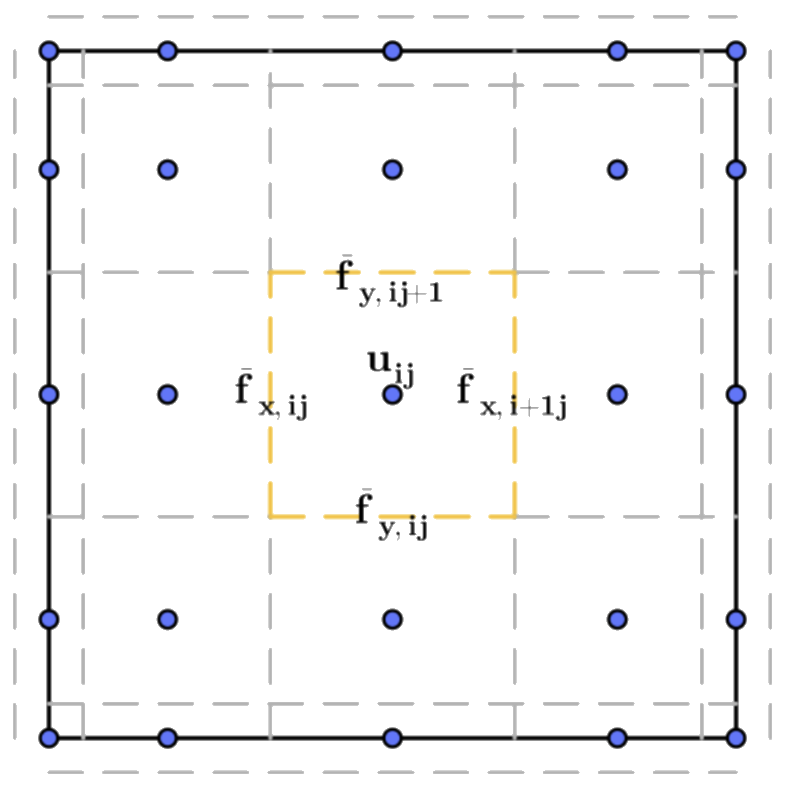
Figure 1: Illustration of algebraic subcell fluxes

3.2.2 Enforcing cell entropy stability in higher dimensions

We proceed in a similar manner as in Section 3.1.1 and delve into the discussion of the proposed subcell limiting strategy in the multidimensional setting. In this context, the subcell limited solution can be divided into surface and volume contributions by utilizing the difference operators (31) and (32). Additionally, the semi-discrete cell entropy inequality [18] can also be decomposed into volume and surface contributions:

$$\bm{\mathsf{M}}\frac{{\rm d}\bm{\mathsf{u}}}{{\rm d}{{t}}} =\sum\limits_{k=1}^{2}\underbrace{\bm{\mathsf{\Delta}}_{k}^{\rm vol}\bar{\bm{\mathsf{f}}}_{k}}_{\bar{\bm{\mathsf{q}}}^{\rm vol}_{k}}+\underbrace{\bm{\mathsf{\Delta}}_{k}^{\rm surf}\bar{\bm{\mathsf{f}}}_{k}}_{\bar{\bm{\mathsf{q}}}^{\rm surf}_{k}},$$ (38)

$$\bm{\mathsf{v}}^{T}\bm{\mathsf{M}}\frac{{\rm d}\bm{\mathsf{u}}}{{\rm d}{{t}}} \leq\sum\limits_{k=1}^{2}\underbrace{\bm{\mathsf{1}}^{T}\bm{\mathsf{B}}_{k}\bm{\mathsf{\psi}}_{k}}_{\bm{\mathsf{P}}^{\rm vol}_{k}}-\underbrace{\left(\bm{\mathsf{v}}_{f}\right)^{T}\bm{\mathsf{B}}_{k}\bm{\mathsf{f}}_{k}^{*}}_{\bm{\mathsf{P}}^{\rm surf}_{k}}.$$ (39)

In addition to enforce the cell entropy inequality separately on the volume and surface contributions, we adopt a dimension-by-dimension approach to enforce the inequality:

$$\bm{\mathsf{v}}^{T}\bar{\bm{\mathsf{q}}}^{\rm vol}_{k}\leq\bm{\mathsf{P}}^{\rm vol}_{k},\qquad\bm{\mathsf{v}}^{T}\bar{\bm{\mathsf{q}}}^{\rm surf}_{k}\leq-\bm{\mathsf{P}}^{\rm surf}_{k},\qquad k=1,2.$$ (40)

Along each dimension $k$, the following identity holds for the surface contributions by (33):

$$\bm{\mathsf{v}}^{T}\bar{\bm{\mathsf{q}}}^{\rm surf}_{k}=\bm{\mathsf{v}}^{T}\bm{\mathsf{\Delta}}_{k}^{\rm vol}\bar{\bm{\mathsf{f}}}_{k}=\left(\bm{\mathsf{v}}_{f}\right)^{T}\bm{\mathsf{B}}_{k}\bm{\mathsf{f}}_{k}^{*}=-\bm{\mathsf{P}}_{k}^{\rm surf}.$$ (41)

As a result, the semi-discrete entropy balance (39) holds for the subcell limited solution if the volume contribution satisfies:

$$\bm{\mathsf{v}}^{T}\bar{\bm{\mathsf{q}}}^{\rm vol}_{k}\leq\bm{\mathsf{P}}^{\rm vol}_{k}.$$ (42)

Through algebraic manipulations, we can write the inequality (42) explicitly in terms of the subcell limiting factors $\bm{\mathsf{l}}_{k}$ as unknowns

$$\bm{\mathsf{l}}_{k}^{T}\left(\underbrace{\left({\bm{\mathsf{\Delta}}_{k}^{\rm vol}}^{T}\bm{\mathsf{v}}\right)^{T}\bar{\bm{\mathsf{f}}}^{\rm H}_{k}}_{\bm{\mathsf{d}}_{k}^{\rm H}}-\underbrace{\left({\bm{\mathsf{\Delta}}_{k}^{\rm vol}}^{T}\bm{\mathsf{v}}\right)^{T}\bar{\bm{\mathsf{f}}}^{\rm L}_{k}}_{\bm{\mathsf{d}}_{k}^{\rm L}}\right)+\bm{1}^{T}\bm{\mathsf{d}}_{k}^{\rm L}\leq\bm{\mathsf{1}}^{T}\bm{\mathsf{B}}_{k}\bm{\mathsf{\psi}}_{k},$$ (43)

Due to the sparsity pattern of $\bm{\mathsf{\Delta}}^{\rm vol}_{k}$, the number of unknowns in the inequalities (43) can be reduced from $\left(N+2\right)\left(N+1\right)$ to $N\left(N+1\right)$. In summary, we want to solve for volume subcell limiting factors in each dimension: $\left\{l_{x,ij}\right\}_{i=1,\dots,N,j=1,\dots,N+1}$, $\left\{l_{y,ij}\right\}_{i=1,\dots,N+1,j=1,\dots,N}$ that satisfies the entropy inequality (43):

$$\sum\limits_{j=1}^{N+1}\sum\limits_{i=1}^{N}\left(\bm{\mathsf{v}}_{ij}-\bm{\mathsf{v}}_{i+1j}\right)^{T}\left(\bar{\bm{\mathsf{f}}}_{x,i+1j}^{\rm H}-\bar{\bm{\mathsf{f}}}_{x,i+1j}^{\rm L}\right)\bm{\mathsf{l}}_{x,i+1j}\leq\bm{1}^{T}\bm{\mathsf{B}}_{x}\bm{\mathsf{\psi}}_{x}-\bm{1}^{T}\bm{\mathsf{d}}_{x}^{\rm L}$$ (44)

$$\sum\limits_{i=1}^{N+1}\sum\limits_{j=1}^{N}\left(\bm{\mathsf{v}}_{ij}-\bm{\mathsf{v}}_{ij+1}\right)^{T}\left(\bar{\bm{\mathsf{f}}}_{y,ij+1}^{\rm H}-\bar{\bm{\mathsf{f}}}_{x,ij+1}^{\rm L}\right)\bm{\mathsf{l}}_{y,i+1j}\leq\bm{1}^{T}\bm{\mathsf{B}}_{y}\bm{\mathsf{\psi}}_{y}-\bm{1}^{T}\bm{\mathsf{d}}_{y}^{\rm L}$$ (45)

Let $\bm{\mathsf{l}}_{x}^{\rm C}$ denote the limiting factors that preserve the convex constraints. Then, the problem of finding suitable subcell limiting factors can be formulated as linear programs for each dimension $k$. We present the linear program in x-direction for brevity:

$$\max\limits_{\bm{\mathsf{l}}_{x,ij}}\quad \sum\limits_{j=1}^{N+1}\sum\limits_{i=2}^{N+1}\bm{\mathsf{l}}_{x,ij}$$ (46a)

s.t. $$\sum\limits_{j=1}^{N+1}\sum\limits_{i=1}^{N}\left(\bm{\mathsf{v}}_{ij}-\bm{\mathsf{v}}_{i+1j}\right)^{T}\left(\bar{\bm{\mathsf{f}}}_{x,i+1j}^{\rm H}-\bar{\bm{\mathsf{f}}}_{x,i+1j}^{\rm L}\right)\bm{\mathsf{l}}_{k,i+1j}\leq\bm{1}^{T}\bm{\mathsf{B}}_{x}\bm{\mathsf{\psi}}_{x}-\bm{1}^{T}\bm{\mathsf{d}}_{x}^{\rm L}$$ (46b)

$$\bm{\mathsf{0}}\leq\bm{\mathsf{l}}_{x,ij}\leq\bm{\mathsf{l}}_{x,ij}^{\rm C}$$ (46c)

The linear program is still of form (28), and the greedy algorithm 1 can still be applied. The solution of this linear program (46) satisfies the following properties:

Theorem 3.3.

The linear program 46 is solvable. The optimal solution to the linear program is locally conservative, satisfies a semi-discrete entropy stability (39), and preserves the given convex constraints enforced by $l^{\rm C}$.

Proof.

The solvability follows from the entropy stability of the low order discretization:

$$\bm{1}^{T}\bm{\mathsf{d}}_{x}^{\rm L}=\left({\bm{\mathsf{\Delta}}_{k}^{\rm vol}}^{T}\bm{\mathsf{v}}\right)^{T}\bar{\bm{\mathsf{f}}}^{\rm L}_{k}\leq\bm{1}^{T}\bm{\mathsf{B}}_{x}\bm{\mathsf{\psi}}_{x}.$$ (47)

The optimal solution is locally conservative by simple algebra:

$$\bm{\mathsf{1}}^{T}\bm{\mathsf{M}}\frac{{\rm d}\bm{\mathsf{u}}}{{\rm d}{{t}}}=\sum\limits_{k=1}^{2}\bm{\mathsf{1}}^{T}\bm{\mathsf{\Delta}}_{k}\bar{\bm{\mathsf{f}}}_{k}=\sum\limits_{k=1}^{2}\bm{\mathsf{1}}^{T}\bm{\mathsf{\Delta}}_{k}^{\rm surf}\bar{\bm{\mathsf{f}}}_{k}=-\sum\limits_{k=1}^{2}\bm{\mathsf{1}}^{T}\bm{\mathsf{B}}_{k}\bm{\mathsf{f}}_{k}^{*},$$ (48)

where we used the identity $\bm{1}^{T}\bm{\mathsf{\Delta}}=\bm{1}^{T}\bm{\mathsf{\Delta}}^{\rm surf}$, along with the assumption (14) that high and low order methods share the same surface contributions. The semi-discrete entropy stability and preservation of convex constraints follows from the constraints (46b) and (46c). ∎

3.3 Incorporating shock capturing

At nonsmooth regions, the volume entropy estimate of the subcell limited solution is expected to dissipate. To account for this, we propose an alternative upper bound as a replacement for (46b) on the volume entropy estimate of the subcell limited solution. This new bound combines the original entropy estimate with the dissipative low order entropy estimate:

$$\bm{\mathsf{v}}^{T}\bm{\mathsf{\Delta}}_{k}^{\rm vol}\bar{\bm{\mathsf{f}}}_{k} \leq\left(1-\epsilon\right)\left[\bm{\mathsf{1}}^{T}\bm{\mathsf{B}}_{k}\bm{\mathsf{\psi}}_{k}-\bm{\mathsf{v}}^{T}\bm{\mathsf{\Delta}}_{k}^{\rm vol}\bar{\bm{\mathsf{f}}}_{k}^{\rm L}\right]+\epsilon\left[\left(1-\beta\right)\bm{\mathsf{1}}^{T}\bm{\mathsf{B}}_{k}\bm{\mathsf{\psi}}_{k}+\beta\bm{\mathsf{v}}^{T}\bm{\mathsf{\Delta}}_{k}^{\rm vol}\bar{\bm{\mathsf{f}}}_{k}^{\rm L}-\bm{\mathsf{v}}^{T}\bm{\mathsf{\Delta}}_{k}^{\rm vol}\bar{\bm{\mathsf{f}}}_{k}^{\rm L}\right]$$

$$=\left(1-\beta\epsilon\right)\left[\bm{\mathsf{1}}^{T}\bm{\mathsf{B}}_{k}\bm{\mathsf{\psi}}_{k}-\bm{\mathsf{v}}^{T}\bm{\mathsf{\Delta}}_{k}^{\rm vol}\bar{\bm{\mathsf{f}}}_{k}^{\rm L}\right],$$ (49)

where $\epsilon\in[0,1]$ is an elementwise modal smoothness factor. In particular, the smoothness factor is defined as [1, 31]:

$$\epsilon=\begin{cases}0,&\text{if }s<s_{0}-\kappa\\ 0.5\left(1-\sin\left(\pi\frac{s-s_{0}}{2\kappa}\right)\right)&\text{if }s\in\left[s_{0}-\kappa,s_{0}+\kappa\right]\\ 1,&\text{if }s<s_{0}+\kappa\end{cases},\quad s=\log_{10}\left(\max\left(\frac{\mu_{N_{p}}^{2}}{\sum\limits_{i=0}^{N_{p}}\mu_{i}^{2}},\frac{\mu_{N_{p}-1}^{2}}{\sum\limits_{i=0}^{N_{p}-1}\mu_{i}^{2}}\right)\right),$$ (50)

where $s$ is the modal smoothness indicator, and $N_{p}=\left(N+1\right)\left(N+1\right)$ is the number of degrees of freedom in an element. We set user-defined parameters $\kappa=1,s_{0}=\log_{10}\left(N^{-4}\right)$ as in [1]. $\left\{\mu_{i}\right\}_{i=0}^{N}$ are the modal coefficients of the polynomial solution in the orthonormal Legendre basis $\left\{\widetilde{L}_{i}\left(x\right)\right\}_{i=0}^{N_{p}}$, such that $u\left(x\right)=\sum\limits_{i=0}^{N}\mu_{i}\widetilde{L}_{i}\left(x\right)$. $\beta\in[0,1]$ is a user-defined parameter that determines the maximum amount of the low-order entropy estimate to blend. When $\beta=0$, the original bound (46b) is recovered. In smooth regions, entropy is conserved in the interior of the element. In nonsmooth regions, the amount of entropy dissipation added is guided by the entropy dissipation from the low-order discretization.

For completeness, we present here the linear program formulation to enforce cell entropy stability with shock capturing:

$$\max\limits_{\bm{\mathsf{l}}_{x,ij}}\quad \sum\limits_{j=1}^{N+1}\sum\limits_{i=2}^{N+1}\bm{\mathsf{l}}_{x,ij}$$ (51a)

s.t. $$\sum\limits_{j=1}^{N+1}\sum\limits_{i=1}^{N}\left(\bm{\mathsf{v}}_{ij}-\bm{\mathsf{v}}_{i+1j}\right)^{T}\left(\bar{\bm{\mathsf{f}}}_{x,i+1j}^{\rm H}-\bar{\bm{\mathsf{f}}}_{x,i+1j}^{\rm L}\right)\bm{\mathsf{l}}_{k,i+1j}\leq\left(1-\beta\epsilon\right)\left[\bm{1}^{T}\bm{\mathsf{B}}_{x}\bm{\mathsf{\psi}}_{x}-\bm{1}^{T}\bm{\mathsf{d}}_{x}^{\rm L}\right]$$ (51b)

$$\bm{\mathsf{0}}\leq\bm{\mathsf{l}}_{x,ij}\leq\bm{\mathsf{l}}_{x,ij}^{\rm C}$$ (51c)

We note that the only difference between the LP formulations (46) and (51) is the upper bound of the cell entropy inequality constraint (46b) and (51b). In future sections, we refer to the condition (51b) with $\beta=0$ as the cell entropy inequality condition. A shock capturing cell entropy stability refers to the same condition with a nonzero value of $\beta$.

3.4 On implementation

The proposed greedy algorithm can be efficiently implemented by first sorting the coefficient vector $\bm{\mathsf{a}}$, and then proceeding with the greedy iterations in the sorted order. It can also be proven that for an index $i$ where $\bm{\mathsf{a}}_{i}$ is non-positive, the optimal solution is $\bm{\mathsf{x}}_{i}=\bm{\mathsf{U}}_{i}$ due to the non-negativity constraint on $\bm{\mathsf{x}}_{i}$. Furthermore, the number of arithmetic operations in Algorithm 1 can be reduced by iteratively accumulating the dot product $\bm{\mathsf{a}}^{T}\bm{\mathsf{x}}$ in each greedy step instead of naively evaluating the dot product at each step. Overall, the number of operations for Algorithm 2 is $O\left(m\log\left(m\right)\right)$, where $m=N\left(N+1\right)$. We note that calculating the coefficient vector $\bm{\mathsf{a}}$ and the right hand side $b$ involves evaluating the entropy variables and entropy potentials, which may be nonlinear functions with respect to the conservative variables $\bm{\mathsf{u}}$ .

However, in practice, numerical issues can arise due to floating-point errors. One of the issues arises due to the division by $\bm{\mathsf{a}}_{i}$. To avoid this, a tolerance $\epsilon_{0}>0$, close to machine epsilon, is set, and indices $i$ where $\bm{\mathsf{a}}_{i}<\epsilon_{0}$ are skipped during greedy iterations. We set $\epsilon_{0}=10^{-14}$ in subsequent numerical experiments.

In summary, Algorithm 2 presents the efficient and robust pseudocode implementation of the proposed limiting strategy. We summarize the proposed subcell limiting strategy that preserves both cell entropy stability and convex constraints in Algorithm 3:

Data: $\bm{\mathsf{a}},b,\bm{\mathsf{U}}\geq\bm{\mathsf{0}},\epsilon_{0}>0$

Result: $\bm{\mathsf{x}}$ optimal solution of LP

$\bm{\mathsf{x}}=\bm{\mathsf{U}}$;

Sort $\bm{\mathsf{a}}$ in decreasing order, and permute $\bm{\mathsf{x}}$ with respect to the order of $\bm{\mathsf{a}}$;

$s=\sum\limits_{j=1}^{N\left(N+1\right)}\bm{\mathsf{a}}_{j}\bm{\mathsf{x}}_{j}$;

if $s\leq b$ then

       return;

for $i=1,\dots,N\left(N+1\right)$ do

       if $\bm{\mathsf{a}}_{i}<\epsilon_{0}$ then

             break;

       $s=s-\bm{\mathsf{a}}_{i}\bm{\mathsf{x}}_{i}$;

       if $s\leq b$ then

             $\bm{\mathsf{x}}_{i}=\frac{b-s}{\bm{\mathsf{a}}_{i}}$;

             break;

      else

             $\bm{\mathsf{x}}_{i}=0.0$;

            

      

Algorithm 2 Efficient implementation of Algorithm 1

Data: $\bm{\mathsf{u}}^{n}$ solution at the current time step

Result: $\bm{\mathsf{u}}^{n+1}$ limited solution at the next time step

Compute $\bm{\mathsf{u}}^{\rm H},\bm{\mathsf{u}}^{\rm L}$ by (11), (13);

for each dimension $k$ do

       Compute algebraic subcell fluxes $\bar{\bm{\mathsf{f}}}_{k}^{\rm H},\bar{\bm{\mathsf{f}}}_{k}^{\rm H}$ by (33), (34), (35);

       Find limiting parameters $\bm{\mathsf{l}}_{k}^{\rm C}$ that satisfies the given convex constraints.

       Find new limiting parameters $\bm{\mathsf{l}}_{k}$ that satisfies the entropy stability using Algorithm 2.

       Construct the limited solution $\bm{\mathsf{u}}^{n+1}$ by (36)

Algorithm 3 The entropy stable and convex constraints preserving limiting strategy

4 Numerical Experiments

In this section, we present various numerical experiments to verify the entropy stability, high-order convergence, and robustness of the proposed limiting strategy . Simulations advance in time with the optimal third-order, three-stage Strong Stability Preserving (SSP) Runge-Kutta, usually referred to as the SSPRK(3,3), scheme [32]. We choose the timestep size according to the timestep condition derived in [27] :

$$\Delta t=\frac{1}{2}\min\limits_{i}\frac{\bm{\mathsf{m}}_{i}}{2\lambda_{i}}.$$ (52)

We note that the time step condition (52) is calculated with the solution at the first SSP stage and is used in all three SSP stages.

In this section, two nonlinear conservation laws are studied: the compressible Euler equation and the KPP problem. To avoid repetition, readers can refer to a previous manuscript [27] for the formula of the compressible Euler equation, and to Section 5.1 of [2] for the formula of the KPP problem.

For the compressible Euler equations presented in [27], the entropy potential is defined as

$$\bm{\psi}\left(\bm{u}\right)=\left(\gamma-1\right)\begin{bmatrix}\rho u\\ \rho v\end{bmatrix}.$$ (53)

We estimate the maximum wavespeed associated with the 1D Riemann problems using the Davis estimate [33] :

$$\lambda_{\max}\left(\bm{u}_{L},\bm{u}_{R},\bm{n}\right)=\max\left(\left|\bm{u}_{L}\cdot\bm{n}\right|+\sqrt{\gamma\frac{p_{L}}{\rho_{L}}},\left|\bm{u}_{R}\cdot\bm{n}\right|+\sqrt{\gamma\frac{p_{R}}{\rho_{R}}}\right).$$ (54)

For comparison, we will investigate some other entropy stabilization techniques for subcell limiting. One popular approach is to enforce a local minimum principle on a modified specific entropy [1, 2]:

$$\phi_{i}\geq\min\limits_{j\in\mathcal{N}\left(i\right)}\phi_{j}^{n},\qquad\phi\left(\bm{u}\right)=\rho^{1-\gamma}e,$$ (55)

where $\mathcal{N}\left(i\right)$ denotes the set of indices $j$ such that the sparse low order operator $\bm{\mathsf{Q}}_{ij}^{\rm L}-{\bm{\mathsf{Q}}_{ij}^{\rm L}}^{T}$ is nonzero. We also consider a relaxed local minimum entropy principle [1]:

$$\phi_{i}\geq\epsilon\min\limits_{j\in\mathcal{N}\left(i\right)}\phi_{j}^{n}+\left(1-\epsilon\right)\phi_{\rm global},$$ (56)

where $\epsilon\in\left[0,1\right]$ is the elementwise modal indicator. Another entropy stabilization proposed in [17] enforced a Tadmor’s entropy condition for subcell fluxes, and we refer this approach as the subcell entropy fix.

In subsequent numerical experiments, we enforce inflow boundary conditions by regarding them as Dirichlet boundary conditions, whose values are given by the initial condition at inflow. Readers can refer to Section 7.1.1 of [6] for the implementation of Dirichlet boundary condition for discontinuous Galerkin discretizations. No boundary conditions are applied at the outflow.

For all numerical experiments, we assume $\beta=0$ in (3.3) unless otherwise explicitly stated.

4.1 On entropy stability

In this section, we will investigate the entropy stability of the proposed limiting strategy using two benchmark test cases to check any entropy violation.

4.1.1 Modified Sod shocktube

We will first consider the modified Sod shock tube problem, which can be found in Section 6.4 of [35]. This problem consists of a left sonic rarefaction wave and is useful for testing whether numerical solutions violate the entropy condition. An entropy-satisfying solution should produce a smooth rarefaction wave. The initial condition for this test problem is given on the domain $\left[0,1\right]$:

$$\bm{u}\left(x\right)=\begin{cases}\bm{u}_{L},\quad&x<0.3\\ \bm{u}_{R},\quad&\text{otherwise}\end{cases},\quad\bm{u}_{L} =\begin{bmatrix}\rho_{L}\\ u_{L}\\ p_{L}\\ \end{bmatrix}=\begin{bmatrix}1.0\\ 0.75\\ 1.0\\ \end{bmatrix},\qquad\bm{u}_{R}=\begin{bmatrix}\rho_{R}\\ u_{R}\\ p_{R}\\ \end{bmatrix}=\begin{bmatrix}0.125\\ 0.0\\ 0.1\\ \end{bmatrix},$$ (57)

where we impose inflow boundary conditions at $x=0.0$ and outflow boundary conditions at $x=1.0$.

We discretize the domain using $K=50$ and $K=100$ uniform intervals, with polynomial degree $N=3$, and run the simulation until $T=0.2$. Figure 2 shows the results obtained using four different types of discretizations, where ESDG refers to the nodal entropy stable DG discretizations mentioned in [27]. We observe that the DGSEM solution clearly violates the entropy condition, resulting in a jump discontinuity at the rarefaction wave. On the other hand, the other three discretizations, including the proposed limiting strategy using cell entropy inequality, do not violate the entropy condition and produce a smooth rarefaction wave.

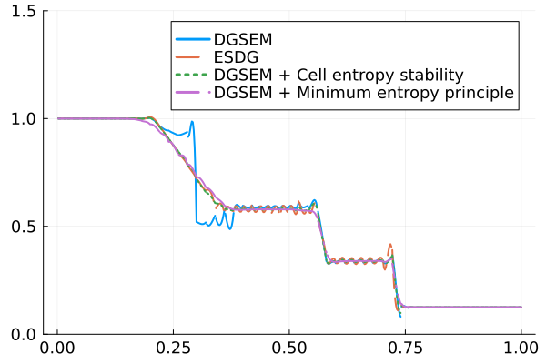
(a) Solutions, $N=3,K=50$

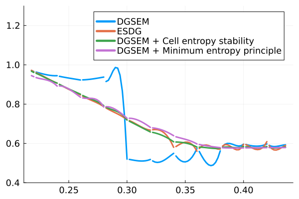
(b) Zoom in view, $N=3,K=50$

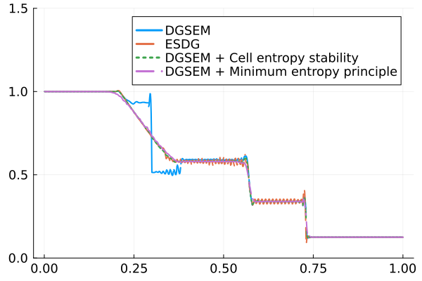
(c) Solutions, $N=3,K=100$

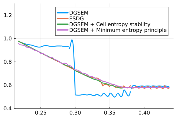
(d) Zoom in view, $N=3,K=100$

Figure 2: Modified Sod shocktube

4.1.2 2D KPP

We next consider the 2D KPP problem [36], where typical high-order methods like DGSEM will converge to non-entropic solutions. We set up the problem using the same initial condition as in [2]. We adopt the blending function and parameters in [31] for shock capturing to eliminate oscillations near shocks for the DGSEM discretizations. In particular, we define the elementwise blending function $\alpha\in\left[0,1\right]$, with

$$\alpha=\frac{1}{1+\exp\left(\frac{-s}{\tau}\left(\epsilon-\tau\right)\right)},\qquad s=\ln\left(\frac{1-0.0001}{0.0001}\right),\qquad\tau=0.5\cdot 10^{-1.8\left(N+1\right)^{0.25}}$$ (58)

where $\epsilon$ is the modal smoothness factor as defined in (50), $s$ is the sharpness factor, and $\tau$ is a threshold value. Then, we apply shock capturing by upper bounding the subcell limiting factors $\bar{l}_{i}$, who are solutions of (46), over each element by the elementwise blending function [27]:

$$l_{i}=\min\left(\bar{l}_{i},1-\alpha\right),$$ (59)

so that an arbitrary amount of the low-order method may be blended in near shocks, or when $\alpha$ is near $1$.

The domain $\left[0,2\right]\times\left[0,2\right]$ is discretized into uniform quadrilateral elements by dividing the $x$ and $y$ directions with $K_{\rm 1D},K_{\rm 1D}$ uniform intervals. We plot the values in the range $\left[-0.5,12\right]$. Figure 3 shows the solutions obtained using DGSEM with and without the proposed entropy limiting when $N=3$. We refine the mesh from $K_{\rm 1D}=64$ to $K_{\rm 1D}=128$ to check the convergence behaviour. We observe that DGSEM without the proposed entropy limiter converges to a non-entropic solution with nonentropic artifacts, which is similarly observed in [2]. On the other hand, the addition of the proposed cell entropy limiter results in a correct entropic solution.

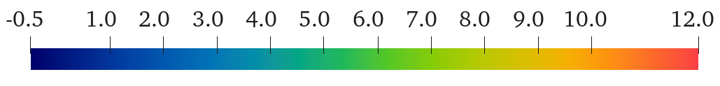
(a) DGSEM, $N=3,K=64$

(b) DGSEM with cell entropy inequality, $N=3,K=64$

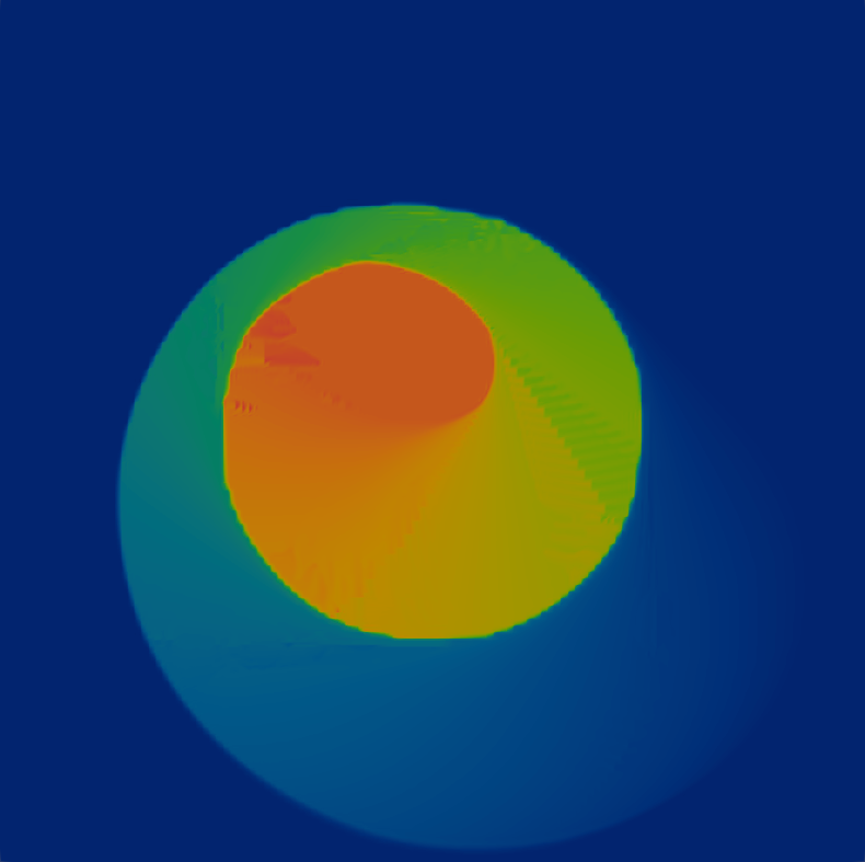
(c) DGSEM, $N=3,K=128$

(d) DGSEM with cell entropy inequality, $N=3,K=128$

Figure 3: 2D KPP problem

4.2 High order accuracy

In this section, we verify the convergence of the subcell limited solution with cell entropy inequality and no additional convex constraints. In particular, we assume $l^{\rm C}=1$. We examine the convergence of the limited solution using the proposed strategy in 2D with the isentropic vortex test case for the compressible Euler equation [37]. Details of the analytical solution can be found in Section 8.2.1 of [27]. The strength of the vortex is set to $\beta_{\rm vortex}=5.0$, such that no positivity limiting is needed. Periodic boundary conditions are imposed, and the simulation is run until $T=1.0$. The domain $\left[0,20\right]\times\left[0,10\right]$ is decomposed into uniform quadrilateral elements by discretizing the $x$ and $y$ directions with $2K_{\rm 1D}$ and $K_{\rm 1D}$ uniform intervals, respectively.

We evaluate the relative $L^{2}$ errors in the conservative variables using LGL quadrature:

$$\frac{\left[\bm{\mathsf{1}}^{T}\bm{\mathsf{M}}\left(\bm{\rho}^{n}-\bm{\rho}\right)^{2}\right]^{1/2}}{\left[\bm{\mathsf{1}}^{T}\bm{\mathsf{M}}\bm{\rho}^{2}\right]^{1/2}}+\frac{\left[\bm{\mathsf{1}}^{T}\bm{\mathsf{M}}\left(\bm{\rho u}^{n}-\bm{\rho u}\right)^{2}\right]^{1/2}}{\left[\bm{\mathsf{1}}^{T}\bm{\mathsf{M}}\left(\bm{\rho u}\right)^{2}\right]^{1/2}}+\frac{\left[\bm{\mathsf{1}}^{T}\bm{\mathsf{M}}\left(\bm{\rho v}^{n}-\bm{\rho v}\right)^{2}\right]^{1/2}}{\left[\bm{\mathsf{1}}^{T}\bm{\mathsf{M}}\left(\bm{\rho v}\right)^{2}\right]^{1/2}}+\frac{\left[\bm{\mathsf{1}}^{T}\bm{\mathsf{M}}\left(\bm{E}^{n}-\bm{E}\right)^{2}\right]^{1/2}}{\left[\bm{\mathsf{1}}^{T}\bm{\mathsf{M}}\bm{E}^{2}\right]^{1/2}},$$ (60)

where the numerical solutions and exact solutions evaluated at quadrature nodes are denoted by $\bm{u}^{n}$ and $\bm{u}$ respectively.

Table 1 shows that the subcell limited solution with cell entropy stability yields an asymptotic convergence rate between $O\left(h^{N+1/2}\right)$ and $O\left(h^{N+1}\right)$. On the other hand, Tables 2 and 3 show that the minimum entropy principle-limited solutions have at most an $O\left(h\right)$ convergence rate and at most an $O\left(h^{2}\right)$ rate after relaxation for any polynomial order $N$ . We note that the proposed strategy of enforcing cell entropy stability does not provably preserve high order accuracy for smooth problems. This section only provides numerical evidence of high-order accuracy.

	$N=1$		$N=2$		$N=3$		$N=4$
K	$L^{2}$ error	Rate	$L^{2}$ error	Rate	$L^{2}$ error	Rate	$L^{2}$ error	Rate
5	$1.183\times 10^{0}$		$6.935\times 10^{-1}$		$2.498\times 10^{-1}$		$1.587\times 10^{-1}$
10	$7.722\times 10^{-1}$	0.62	$1.785\times 10^{-1}$	1.96	$7.083\times 10^{-2}$	1.82	$2.000\times 10^{-2}$	2.99
20	$3.327\times 10^{-1}$	1.22	$4.126\times 10^{-2}$	1.11	$8.898\times 10^{-3}$	2.99	$9.557\times 10^{-4}$	4.39
40	$1.118\times 10^{-1}$	1.57	$6.714\times 10^{-3}$	2.62	$8.163\times 10^{-4}$	3.45	$3.142\times 10^{-5}$	4.93
80	$3.133\times 10^{-2}$	1.84	$1.210\times 10^{-3}$	2.74	$4.208\times 10^{-5}$	4.28	$1.530\times 10^{-6}$	4.36

Table 1: 2D isentropic vortex, uniform quadrilateral mesh, subcell limiting by enforcing cell entropy inequality

	$N=1$		$N=2$		$N=3$		$N=4$
K	$L^{2}$ error	Rate	$L^{2}$ error	Rate	$L^{2}$ error	Rate	$L^{2}$ error	Rate
5	$1.084\times 10^{0}$		$7.498\times 10^{-1}$		$4.499\times 10^{-1}$		$3.135\times 10^{-1}$
10	$7.012\times 10^{-1}$	0.63	$3.343\times 10^{-1}$	1.17	$2.109\times 10^{-1}$	1.09	$1.486\times 10^{-1}$	1.08
20	$3.373\times 10^{-1}$	1.06	$1.894\times 10^{-1}$	0.82	$1.092\times 10^{-1}$	0.95	$7.509\times 10^{-2}$	0.98
40	$1.841\times 10^{-1}$	0.87	$9.718\times 10^{-2}$	0.96	$5.956\times 10^{-2}$	0.87	$4.160\times 10^{-2}$	0.85
80	$1.015\times 10^{-1}$	0.86	$5.116\times 10^{-2}$	0.93	$3.186\times 10^{-2}$	0.90	$2.157\times 10^{-2}$	0.95

Table 2: 2D isentropic vortex, uniform quadrilateral mesh, subcell limiting by enforcing minimum entropy principle

	$N=1$		$N=2$		$N=3$		$N=4$
K	$L^{2}$ error	Rate	$L^{2}$ error	Rate	$L^{2}$ error	Rate	$L^{2}$ error	Rate
5	$1.086\times 10^{0}$		$7.433\times 10^{-1}$		$4.098\times 10^{-1}$		$2.856\times 10^{-1}$
10	$7.047\times 10^{-1}$	0.62	$2.908\times 10^{-1}$	1.35	$1.785\times 10^{-1}$	1.20	$1.109\times 10^{-1}$	1.36
20	$3.154\times 10^{-1}$	1.16	$1.203\times 10^{-1}$	1.27	$5.464\times 10^{-2}$	1.71	$3.352\times 10^{-2}$	1.73
40	$1.295\times 10^{-1}$	1.28	$4.322\times 10^{-2}$	1.48	$1.863\times 10^{-2}$	1.55	$1.532\times 10^{-2}$	1.13
80	$4.500\times 10^{-2}$	1.52	$1.869\times 10^{-2}$	1.21	$6.614\times 10^{-3}$	1.49	$6.120\times 10^{-3}$	1.31

Table 3: 2D isentropic vortex, uniform quadrilateral mesh, subcell limiting by enforcing relaxed minimum entropy principle

4.3 Kelvin-Helmholtz Instability

We now consider the Kelvin-Helmholtz instability [20] to study the behaviour of the proposed limiting strategy in presence of turbulence. The domain is $\left[-1,1\right]^{2}$ with initial condition:

$$\bm{u}\left(x\right)=\begin{bmatrix}\rho\\ u\\ v\\ p\end{bmatrix}=\begin{bmatrix}0.5+0.75B\left(x,y\right)\\ 0.5\left(B\left(x,y\right)-1\right)\\ 0.1\sin\left(2\pi x\right)\\ 1\end{bmatrix},\qquad B\left(x,y\right)=\tanh\left(15y+7.5\right)-\tanh\left(15y-7.5\right).$$ (61)

We approximate the solution using degree $N=3$ polynomials, and the domain is discretized into $80\times 80$ uniform quadrilateral elements. We ran the simulation until $T=10.0$, and plotted the density in the range of $\left[0.5,2.5\right]$ in a logarithmic scale for better visibility. For this set of simulations, we enforce the cell entropy inequality (39) and relaxed positivity conditions on the density and internal energy

$$\rho\left(\bm{\mathsf{u}}_{i}\right)\geq 0.5\rho\left(\bm{\mathsf{u}}^{\rm L}_{i}\right),\qquad\rho e\left(\bm{\mathsf{u}}_{i}\right)\geq 0.5\rho e\left(\bm{\mathsf{u}}^{\rm L}_{i}\right),$$ (62)

using subcell limiting.

We follow [1, 3, 2] to enforce the bounds (62). We illustrate the limiting procedure in 1D for brevity. The subcell limited solution (36) can be rewritten as a convex combination of substates:

$$\bm{\mathsf{u}}_{i}^{n+1}=\frac{1}{2}\underbrace{\left[\bm{\mathsf{u}}_{i}^{\rm L}+l_{i}\frac{\Delta t}{\bm{\mathsf{m}}_{i}}\left(\bar{\bm{\mathsf{f}}}_{i}^{\rm H}-\bar{\bm{\mathsf{f}}}_{i}^{\rm L}\right)\right]}_{\mathcal{A}_{i}\left(l_{i}\right)}+\frac{1}{2}\underbrace{\left[\bm{\mathsf{u}}_{i}^{\rm L}+l_{i-1}\frac{\Delta t}{\bm{\mathsf{m}}_{i}}\left(\bar{\bm{\mathsf{f}}}_{i-1}^{\rm H}-\bar{\bm{\mathsf{f}}}_{i-1}^{\rm L}\right)\right]}_{\mathcal{B}_{i}\left(l_{i-1}\right)},$$ (63)

If the substates satisfy convex constraints, the limited solution will also satisfy the constraints. Then for each node $i$, we need to find the maximum subcell limiting factor $l_{i}^{\rm C}\in\left[0,1\right]$ that satisfies the constraints:

$$\rho\left(\mathcal{A}_{i}\left(l_{i}^{\rm C}\right)\right) \geq 0.5\rho\left(\bm{\mathsf{u}}_{i}^{\rm L}\right),\qquad\ \ \rho\left(\mathcal{B}_{i+1}\left(l_{i}^{\rm C}\right)\right)\geq 0.5\rho\left(\bm{\mathsf{u}}_{i+1}^{\rm L}\right),$$ (64)

$$\rho e\left(\mathcal{A}_{i}\left(l_{i}^{\rm C}\right)\right) \geq 0.5\rho e\left(\bm{\mathsf{u}}_{i}^{\rm L}\right),\qquad\rho e\left(\mathcal{B}_{i+1}\left(l_{i}^{\rm C}\right)\right)\geq 0.5\rho e\left(\bm{\mathsf{u}}_{i+1}^{\rm L}\right).$$ (65)

The constraints on density (64) are linear inequalities with a closed-form solution, and the constraints on internal energy (65) can be transformed into quadratic inequalities. Readers can refer to [27] for the explicit formula of the limiting factors.

Figure 4 shows the proposed limiting strategy applied to DGSEM. We observe the simulation is robust and resolving fine-scale turbulence features. Additionally, we apply the proposed limiting strategy to nodal entropy-stable discontinuous Galerkin (ESDG)[27] for comparison, as shown in Figure 5. The proposed limiting preserves the semi-discrete entropy inequality of ESDG discretizations. Although the same types of constraints are applied through subcell limiting, the turbulence structures of both solutions are visually different. In other words, the choice of the high-order scheme in the proposed limiting strategy may have a significant impact on the solution.

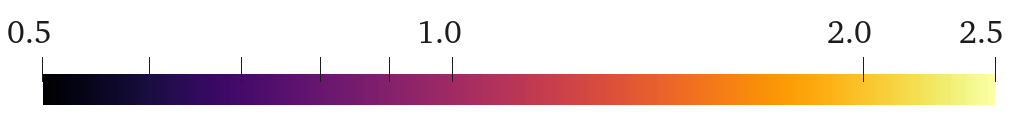
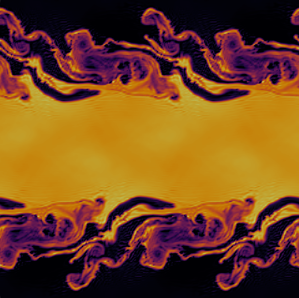
(a) $T=5.0$

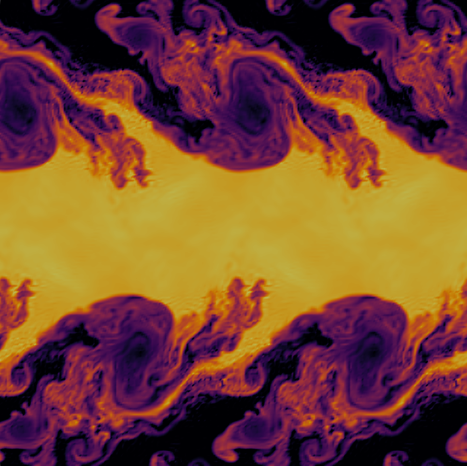
(b) $T=7.5$

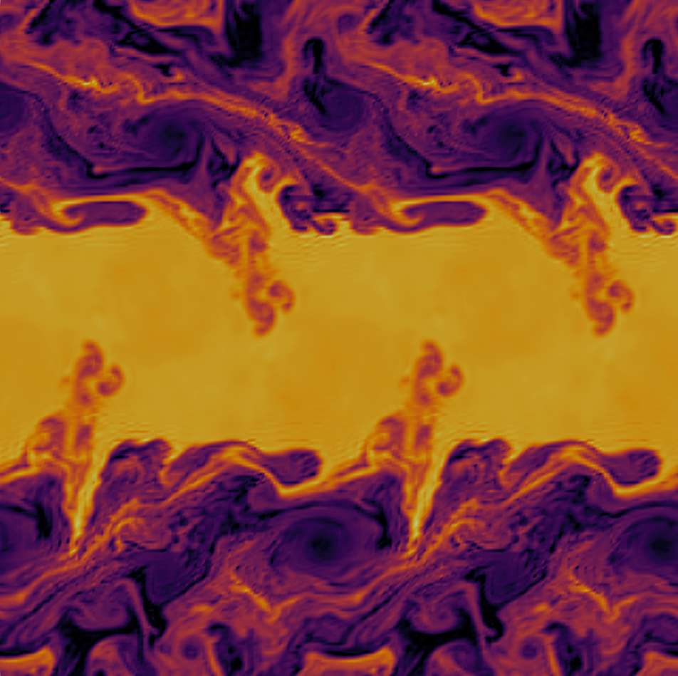
(c) $T=10.0$

Figure 4: Kelvin-Helmholtz Instability, DGSEM limited with relaxed positivity constraints (62) and the cell entropy inequality (39) using subcell limiter

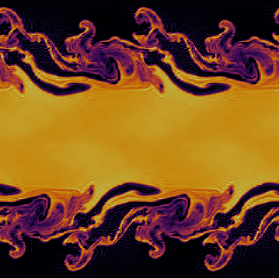
(a) $T=5.0$

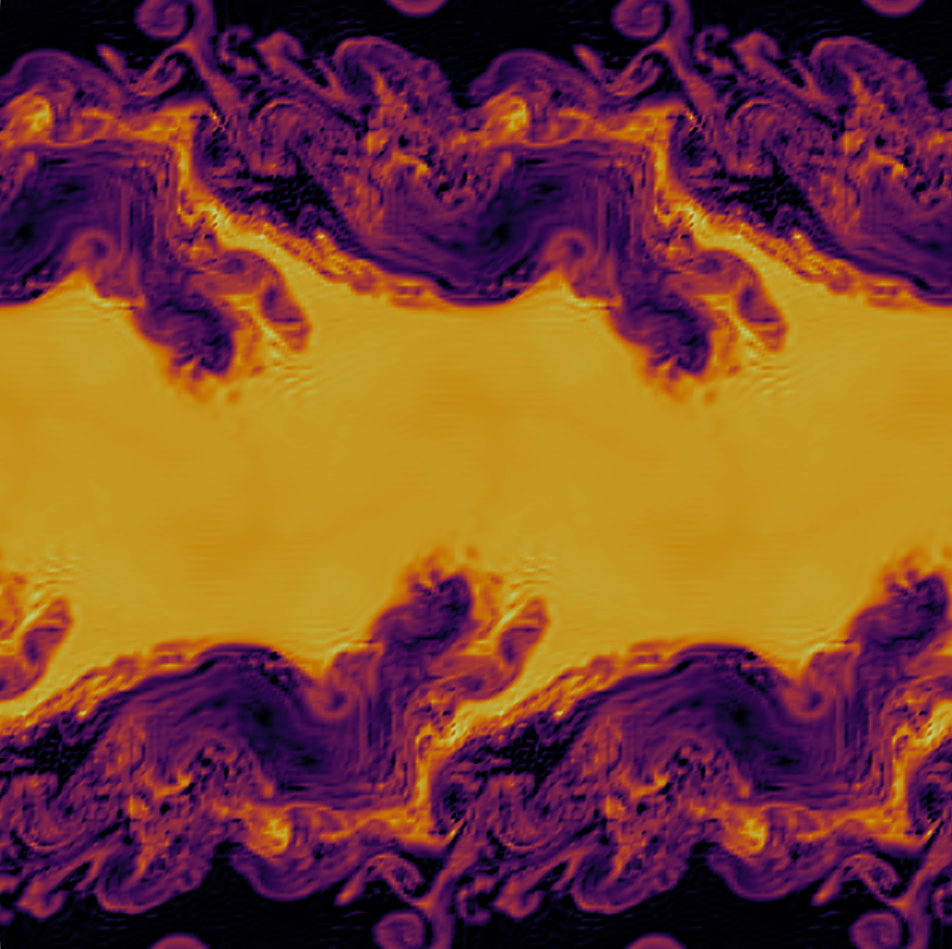
(b) $T=7.5$

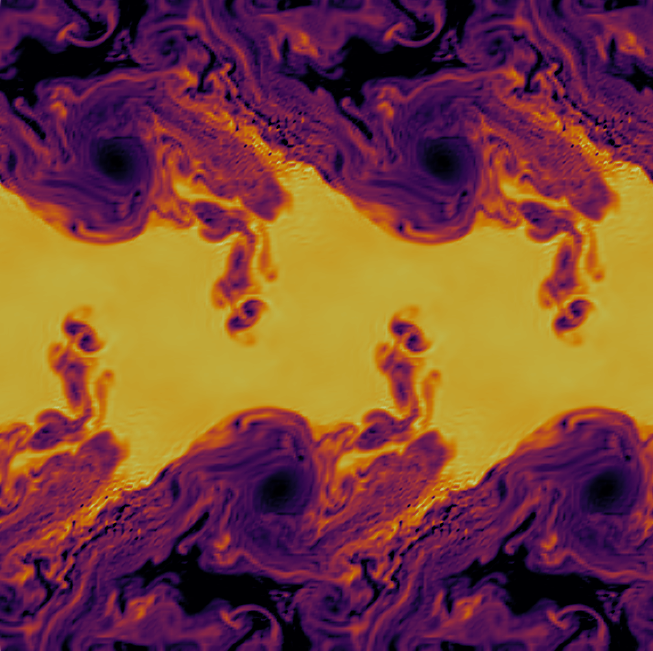
(c) $T=10.0$

Figure 5: Kelvin-Helmholtz Instability, ESDG limited with relaxed positivity constraints (62) and the cell entropy inequality (39) using subcell limiter

4.4 Astrophysical jet

We conclude the experiments by running the astrophysical jet test case proposed by Ha et al.[38] for the compressible Euler equation. This test case involves a high Mach number of ${\rm Ma}\approx 2000$ and strong shocks, making it ideal for testing the robustness of numerical schemes[3, 10]. The domain is $\left[-0.5,0.5\right]^{2}$ initialized with a resting gas, and an inflow boundary condition is imposed on the left of the domain.

$$\textrm{Initial: }\bm{u}=\begin{bmatrix}\rho\\ u\\ v\\ p\end{bmatrix}=\begin{bmatrix}0.5\\ 0.0\\ 0.0\\ 0.4127\end{bmatrix},\qquad\textrm{Inflow: }\bm{u}\left(-0.5,y\right)=\begin{bmatrix}\rho\\ u\\ v\\ p\end{bmatrix}=\begin{bmatrix}5.0\\ 800.0\\ 0.0\\ 0.4127\end{bmatrix}\textrm{ for }y\in\left[-0.05,0.05\right].$$ (66)

We approximate the solution using degree $N=3$ polynomials, and the domain was discretized into $150\times 150$ uniform quadrilateral elements, as constructed in Section 4.1.2. We plotted the density in the range of $\left[0.01,30.0\right]$ in a logarithmic scale for better visibility. All simulations were run until the end time of $T=0.001$.

We first consider enforcing a TVD-like bound on density that depends on the low order update

$$\rho\left(\bm{\mathsf{u}}_{i}\right)\in\left[\rho_{i}^{\min},\rho_{i}^{\max}\right],\qquad\rho_{i}^{\min}=\min\limits_{j\in\mathcal{N}\left(i\right)}\rho\left(\bm{\mathsf{u}}_{i}^{\rm L}\right),\qquad\rho_{i}^{\max}=\max\limits_{j\in\mathcal{N}\left(i\right)}\rho\left(\bm{\mathsf{u}}_{i}^{\rm L}\right),$$ (67)

along with a relaxed positivity condition on the internal energy (62) and the proposed cell entropy inequality (51b). We follow Section 4.3 to enforce the bounds (67) and (62) with subcell limiting. Instead of the relaxed positivity bound (64), we enforce a TVD-like bound on density:

$$\rho\left(\mathcal{A}_{i}\left(l_{i}^{\rm C}\right)\right) \in\left[\rho_{i}^{\min},\rho_{i}^{\max}\right],\qquad\rho\left(\mathcal{B}_{i+1}\left(l_{i}^{\rm C}\right)\right)\in\left[\rho_{i+1}^{\min},\rho_{i+1}^{\max}\right],$$ (68)

which is a linear constraint with a closed form solution of $l_{i}^{C}$. The constraints on density (68) and internal energy (65) can be satisfied under explicit formulas in [27]. Figure 6 shows that the simulation remain robust in the presence of strong shocks.

Next, we study the effect of the relaxation factor $\beta$ in the cell entropy inequality (3.3). For this set of simulations, we only enfroce relaxed positivity conditions on the density and internal energy (62) in addition to the shock capturing cell entropy inequality with different relaxation factors $\beta$. Figure 7 compares the results with $\beta=1.0,0.1,0.01,$ and $0.0$. In other words, the results have at most $100\%,10\%,1\%,$ and $0\%$ low-order cell entropy dissipation blended into the enforced cell entropy bound.

As the relaxation factor $\beta$ decreases, finer-scale features are resolved due to reduced numerical dissipation. However, we observe the appearance of the carbuncle effect when $\beta=0.01$ and $\beta=0.0$, and similarly when using the minimum entropy principle instead of the shock capturing cell entropy inequality, as shown in Figure 8(c). This suggests that the carbuncle effect is not due only to a loss of entropy stability, but rather a lack of sufficient dissipation near shocks. The qualitative behavior of the flow changes significantly with different values of $\beta$, indicating a high sensitivity of the limited solution to the choice of $\beta$.

The final comparison is between

1. The DGSEM discretization limited with the relaxed positivity bound (62) and cell entropy inequality (39) using a subcell limiter, as shown in Figure 7 when $\beta=0$.

2. The ESDG discretization limited with the relaxed positivity bound (62) using an elementwise Zhang-Shu limiter, as shown in Figure 8(b).

3. The ESDG discretization limited with the relaxed positivity bound and cell entropy inequality (39) using a subcell limiter, as shown in Figure 8(a).

All solutions satisfy the same relaxed positivity constraints and the cell entropy stability [27]. The main difference is the limited high-order scheme, DGSEM or ESDG, and the types of limiting, Zhang-Shu or subcell, used. It is observed that the Zhang-Shu limited ESDG solution does not exhibit the carbuncle effect that is present in the subcell limited solution enforcing the cell entropy inequality. This can be partially explained by the fact that the Zhang-Shu limiter is more dissipative than the subcell limiter, and this numerical dissipation is sufficient to eliminate the carbuncle near the shock in this particular test case.

Comparing Figure 7 when $\beta=0$ and Figure 8(a), we observe different turbulence structures when the proposed subcell limiting strategy is applied to DGSEM and ESDG, respectively. This further supports our observation in Section 4.3 that the choice of a high-order scheme in the proposed limiting strategy may have a significant impact on the solution.

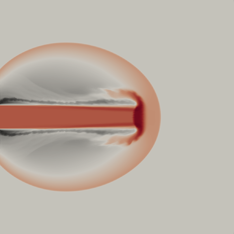
Figure 6: Astrophysical jet, DGSEM limited with TVD-like constraints (68), (65) and the cell entropy inequality (39)

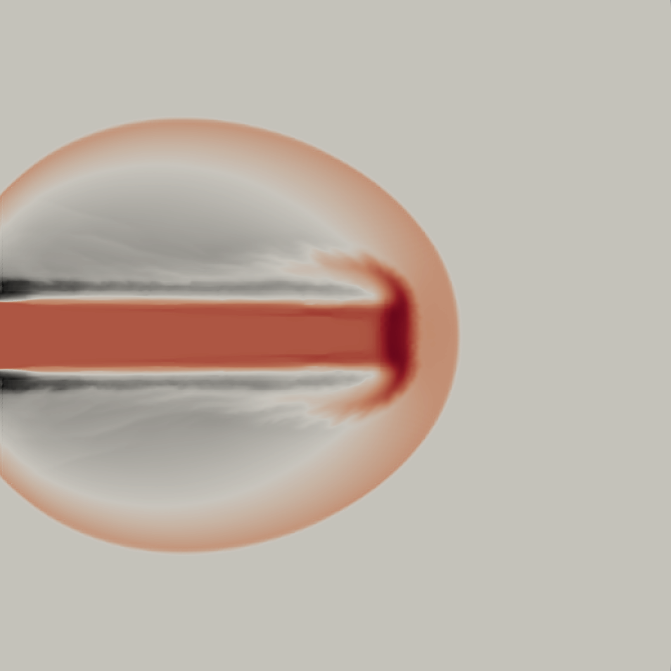
(a) $\beta=1.0$

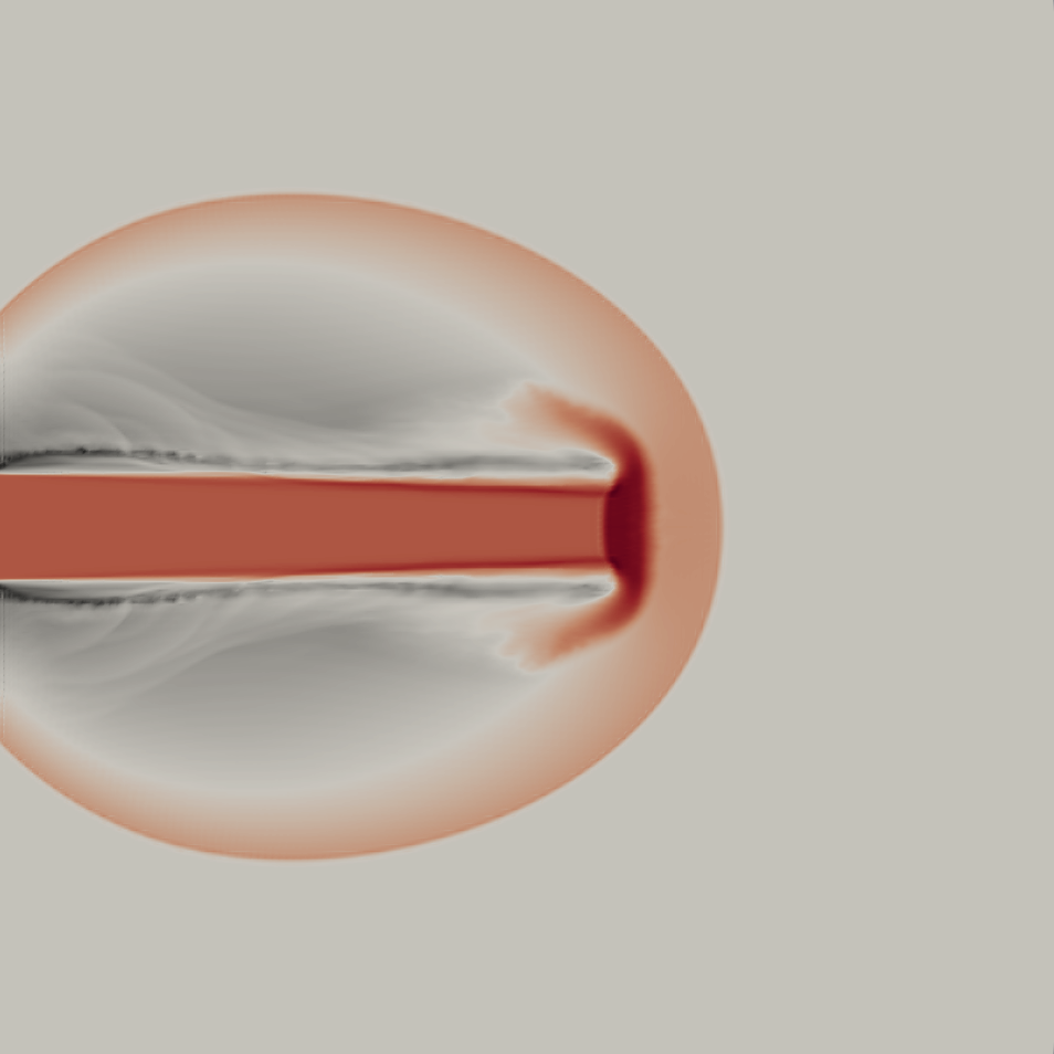
(b) $\beta=0.1$

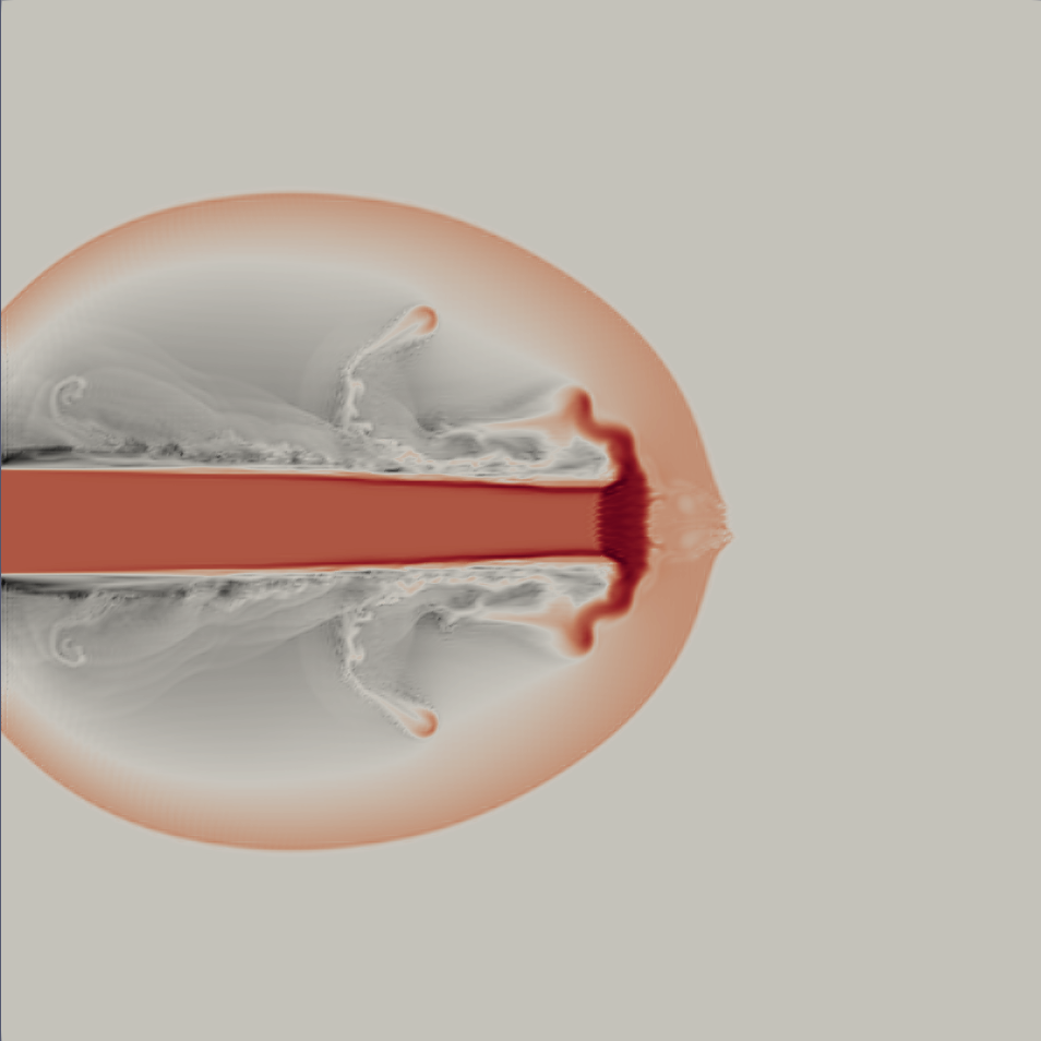
(c) $\beta=0.01$

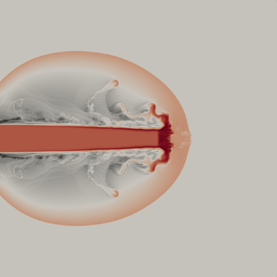
(d) $\beta=0.0$

Figure 7: Astrophysical jet, DGSEM limited with relaxed positivity constraints (62) and the shock capturing cell entropy inequality (3.3)

5 Conclusion

In this paper, we introduce a novel subcell limiting strategy to ensure semi-discrete entropy stability. We formulate the limiting procedure as a linear program that can be solved efficiently using a deterministic greedy algorithm. The resulting subcell limited solution is high order accurate and semi-discretely entropy stable, and can be combined with other subcell limiters to preserve general convex constraints.

Appendix A Astrophysical jets

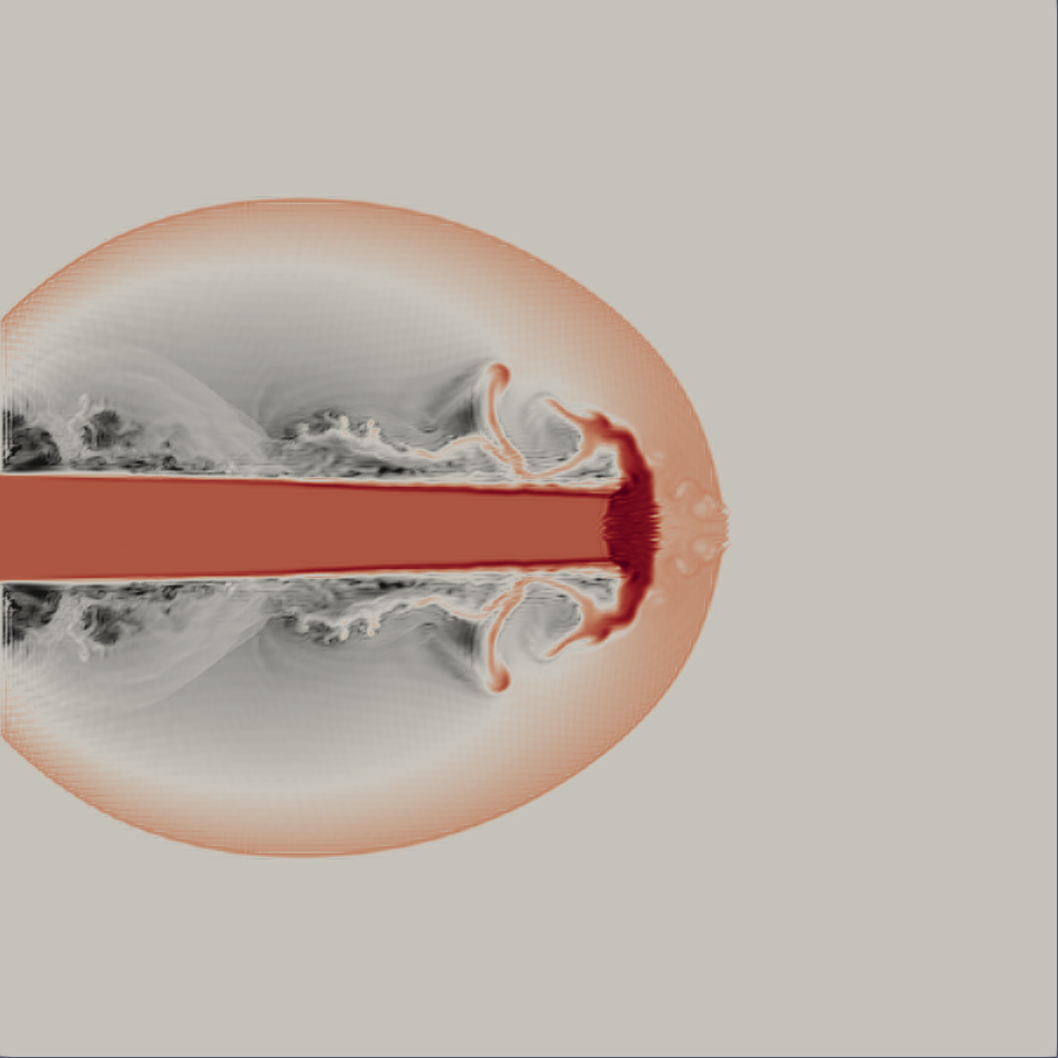
(a) (a) ESDG limited with relaxed positivity constraint (62) and cell entropy inequality (39) using subcell limiter

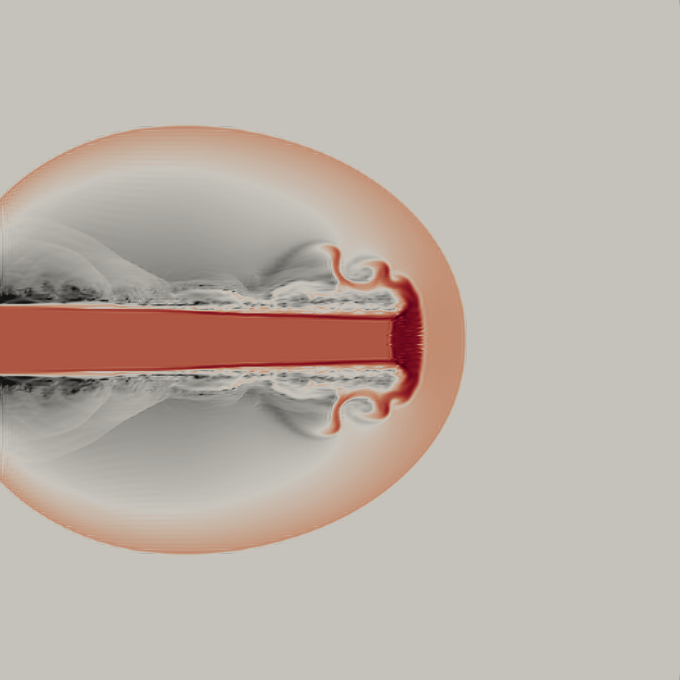
(b) (b) ESDG limited with relaxed positivity constraint (62) using Zhang-Shu limiter [27]

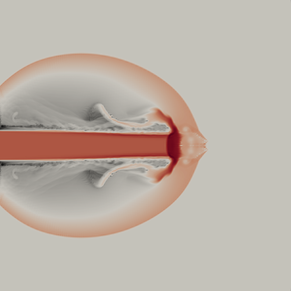
(c) (c) DGSEM limited with relaxed positivity constraint (62) and minimum entropy principle (55) using subcell limiter

Figure 8: Astrophysical jet

References

- [1] W. Pazner, Sparse invariant domain preserving discontinuous Galerkin methods with subcell convex limiting, Computer Methods in Applied Mechanics and Engineering 382 (2021) 113876.
- [2] A. M. Rueda-Ramírez, W. Pazner, G. J. Gassner, Subcell limiting strategies for discontinuous Galerkin spectral element methods, Computers & Fluids 247 (2022) 105627.
- [3] A. M. Rueda-Ramírez, B. Bolm, D. Kuzmin, G. J. Gassner, Monolithic Convex Limiting for Legendre-Gauss-Lobatto Discontinuous Galerkin Spectral Element Methods, arXiv preprint arXiv:2303.00374 (2023).
- [4] J. Slotnick, A. Khodadoust, J. Alonso, D. Darmofal, W. Gropp, E. Lurie, CFD vision 2030 study: a path to revolutionary computational aerosciences, Tech. rep., NASA (2014).
- [5] Z. J. Wang, K. Fidkowski, R. Abgrall, F. Bassi, D. Caraeni, A. Cary, H. Deconinck, R. Hartmann, K. Hillewaert, H. T. Huynh, et al., High-order CFD methods: current status and perspective, International Journal for Numerical Methods in Fluids 72 (8) (2013) 811–845.
- [6] J. S. Hesthaven, T. Warburton, Nodal discontinuous Galerkin methods: algorithms, analysis, and applications, Springer Science & Business Media, 2007.
- [7] L. Krivodonova, Limiters for high-order discontinuous Galerkin methods, Journal of Computational Physics 226 (1) (2007) 879–896.
- [8] P.-O. Persson, J. Peraire, Sub-cell shock capturing for discontinuous Galerkin methods, in: 44th AIAA Aerospace Sciences Meeting and Exhibit, 2006, p. 112.
- [9] X. Zhang, C.-W. Shu, On maximum-principle-satisfying high order schemes for scalar conservation laws, Journal of Computational Physics 229 (9) (2010) 3091–3120.
- [10] X. Zhang, C.-W. Shu, On positivity-preserving high order discontinuous Galerkin schemes for compressible Euler equations on rectangular meshes, Journal of Computational Physics 229 (23) (2010) 8918–8934.
- [11] X. Zhang, C.-W. Shu, A minimum entropy principle of high order schemes for gas dynamics equations, Numerische Mathematik 121 (3) (2012) 545–563.
- [12] J. P. Boris, D. L. Book, Flux-corrected transport. I. SHASTA, a fluid transport algorithm that works, Journal of computational physics 11 (1) (1973) 38–69.
- [13] S. T. Zalesak, Fully multidimensional flux-corrected transport algorithms for fluids, Journal of computational physics 31 (3) (1979) 335–362.
- [14] D. Kuzmin, R. Löhner, S. Turek, Flux-corrected transport: principles, algorithms, and applications, Springer, 2012.
- [15] J.-L. Guermond, B. Popov, Invariant domains and first-order continuous finite element approximation for hyperbolic systems, SIAM Journal on Numerical Analysis 54 (4) (2016) 2466–2489.
- [16] C. Lohmann, D. Kuzmin, J. N. Shadid, S. Mabuza, Flux-corrected transport algorithms for continuous Galerkin methods based on high order Bernstein finite elements, Journal of Computational Physics 344 (2017) 151–186.
- [17] D. Kuzmin, H. Hajduk, A. Rupp, Limiter-based entropy stabilization of semi-discrete and fully discrete schemes for nonlinear hyperbolic problems, Computer Methods in Applied Mechanics and Engineering 389 (2022) 114428.
- [18] J. Chan, On discretely entropy conservative and entropy stable discontinuous Galerkin methods, Journal of Computational Physics 362 (2018) 346–374.
- [19] J. Chan, L. C. Wilcox, On discretely entropy stable weight-adjusted discontinuous Galerkin methods: curvilinear meshes, Journal of Computational Physics 378 (2019) 366–393.
- [20] J. Chan, Y. Lin, T. Warburton, Entropy stable modal discontinuous Galerkin schemes and wall boundary conditions for the compressible Navier-Stokes equations, Journal of Computational Physics 448 (2022) 110723.
- [21] M. H. Carpenter, T. C. Fisher, E. J. Nielsen, S. H. Frankel, Entropy stable spectral collocation schemes for the Navier-Stokes equations: Discontinuous interfaces, SIAM Journal on Scientific Computing 36 (5) (2014) B835–B867.
- [22] G. J. Gassner, A skew-symmetric discontinuous Galerkin spectral element discretization and its relation to SBP-SAT finite difference methods, SIAM Journal on Scientific Computing 35 (3) (2013) A1233–A1253.
- [23] G. J. Gassner, A. R. Winters, D. A. Kopriva, Split form nodal discontinuous Galerkin schemes with summation-by-parts property for the compressible Euler equations, Journal of Computational Physics 327 (2016) 39–66.
- [24] T. Chen, C.-W. Shu, Entropy stable high order discontinuous Galerkin methods with suitable quadrature rules for hyperbolic conservation laws, Journal of Computational Physics 345 (2017) 427–461.
- [25] R. Abgrall, A general framework to construct schemes satisfying additional conservation relations. Application to entropy conservative and entropy dissipative schemes, Journal of Computational Physics 372 (2018) 640–666.
- [26] R. Abgrall, P. Öffner, H. Ranocha, Reinterpretation and extension of entropy correction terms for residual distribution and discontinuous Galerkin schemes: application to structure preserving discretization, Journal of Computational Physics 453 (2022) 110955.
- [27] Y. Lin, J. Chan, I. Tomas, A positivity preserving strategy for entropy stable discontinuous Galerkin discretizations of the compressible Euler and Navier-Stokes equations, Journal of Computational Physics 475 (2023) 111850.
- [28] H. Hajduk, Monolithic convex limiting in discontinuous Galerkin discretizations of hyperbolic conservation laws, Computers & Mathematics with Applications 87 (2021) 120–138.
- [29] G. B. Dantzig, Discrete-variable extremum problems, Operations research 5 (2) (1957) 266–288.
- [30] A. Mateo-Gabín, A. M. Rueda-Ramírez, E. Valero, G. Rubio, A flux-differencing formulation with gauss nodes, Journal of Computational Physics (2023) 112298.
- [31] S. Hennemann, A. M. Rueda-Ramírez, F. J. Hindenlang, G. J. Gassner, A provably entropy stable subcell shock capturing approach for high order split form DG for the compressible Euler equations, Journal of Computational Physics 426 (2021) 109935.
- [32] S. Gottlieb, C.-W. Shu, E. Tadmor, Strong stability-preserving high-order time discretization methods, SIAM review 43 (1) (2001) 89–112.
- [33] S. Davis, Simplified second-order Godunov-type methods, SIAM Journal on Scientific and Statistical Computing 9 (3) (1988) 445–473.
- [34] J.-L. Guermond, B. Popov, Fast estimation from above of the maximum wave speed in the Riemann problem for the Euler equations, Journal of Computational Physics 321 (2016) 908–926.
- [35] E. F. Toro, Riemann solvers and numerical methods for fluid dynamics: a practical introduction, Springer Science & Business Media, 2013.
- [36] A. Kurganov, G. Petrova, B. Popov, Adaptive semidiscrete central-upwind schemes for nonconvex hyperbolic conservation laws, SIAM Journal on Scientific Computing 29 (6) (2007) 2381–2401.
- [37] C.-W. Shu, S. Osher, Efficient implementation of essentially non-oscillatory shock-capturing schemes, Journal of computational physics 77 (2) (1988) 439–471.
- [38] Y. Ha, C. L. Gardner, A. Gelb, C.-W. Shu, Numerical simulation of high Mach number astrophysical jets with radiative cooling, Journal of Scientific Computing 24 (2005) 29–44.