Islands and dynamics at the interface

Abstract

We investigate a family of models described by two holographic CFT₂s coupled along a shared interface. The bulk dual geometry consists of two AdS₃ spacetimes truncated by a shared Karch-Randall end-of-the-world (EOW) brane. A lower dimensional effective model comprising of JT gravity coupled to two flat CFT₂ baths is subsequently realized by considering small fluctuations on the EOW brane and implementing a partial Randall-Sundrum reduction where the transverse fluctuations of the EOW brane are identified as the dilaton field. We compute the generalized entanglement entropy for bipartite states through the island prescription in the effective lower dimensional picture and obtain precise agreement in the limit of large brane tension with the corresponding doubly holographic computations in the bulk geometry. Furthermore, we obtain the corresponding Page curves for the Hawking radiation in this JT braneworld.

1 Introduction

In recent years the remarkable progress towards a possible resolution of the black hole information loss paradox in toy models has garnered intense research focus. This development involved the inclusion of bulk regions termed “islands”, in the entanglement wedge for subsystems in radiation baths at late times Penington:2019npb ; Penington:2019kki ; Almheiri:2019hni ; Almheiri:2019qdq ; Almheiri:2019yqk . The appearance of these islands ensure that the von Neumann entropy of the Hawking radiation follows the Page curve Page:1993wv ; Page:1993df ; Page:2013dx . The crucial ingredient in this island formalism is the incorporation of replica wormhole saddles dominant at late times, in the gravitational path integral for the Rényi entanglement entropy. A more natural way to understand this island formalism was provided through the doubly holographic description Almheiri:2019hni ; Sully:2020pza ; Rozali:2019day ; Chen:2020uac ; Chen:2020hmv ; Grimaldi:2022suv ; Suzuki:2022xwv in which the radiation baths are described by holographic CFTs dual to a bulk geometry. The island formula then emerges from the standard holographic characterization of the entanglement entropy through the (H)RT prescription in the corresponding higher dimensional bulk geometry.

The above doubly holographic interpretation of the island formula was explored in Deng:2020ent ; Chu:2021gdb in the context of an extension of the AdS₃/BCFT₂ Takayanagi:2011zk ; Fujita:2011fp ; Rozali:2019day ; Sully:2020pza ; Kastikainen:2021ybu duality through the inclusion of additional defect conformal matter on the end-of-the-world (EOW) brane. In this defect AdS₃/BCFT₂ framework the equivalence of the quantum corrected RT formula, termed as the defect extremal surface formula, in the $3d$ bulk geometry with the corresponding island formula in the lower dimensional effective $2d$ description could be demonstrated. This doubly holographic description in the defect AdS₃/BCFT₂ framework was further investigated for different mixed state entanglement measures Li:2021dmf ; Basu:2022reu ; Shao:2022gpg ; Lu:2022cgq .

In relation to the above discussion, the Jackiw-Teitelboim (JT) gravity Jackiw:1984je ; Teitelboim:1983ux coupled to a radiation bath in two dimensions has proved to be an interesting solvable model to study the application of the island formula Almheiri:2019qdq ; Penington:2019kki . Recently in Deng:2022yll , the authors have realised this setup through a dimensional reduction of a defect AdS₃ bulk with small transverse fluctuations on the EOW brane. In particular, they have derived the full JT gravity action through a partial dimensional reduction of the $3d$ bulk wedge sandwiched between a virtual zero tension brane and the finite tension EOW brane, by identifying the transverse fluctuations with the dilaton field in the $2d$ effective description. Usual AdS₃/CFT₂ prescription has been utilized in the remaining part of the bulk to obtain the bath CFT₂ on the asymptotic boundary of the AdS₃ geometries. This has provided a $3d$ holographic dual for the JT gravity coupled to a CFT₂ bath.

On a separate note, the doubly holographic description of the island formula has been further investigated in Anous:2022wqh for an interface CFT (ICFT₂) where two CFT₂s on half lines with different central charges were considered to be communicating through a common quantum dot. The holographic bulk for such a field theoretic configuration is described by two truncated AdS₃ geometries with different length scales, sewed together along the constant tension EOW brane. In such a configuration, the equivalence between the island formula and the holographic entanglement entropy has been illustrated for certain bipartite states.

In this context, lifting the constraint of the rigidity of the EOW brane in the ICFT₂ setup could lead to interesting physics. In the present article this configuration has been investigated where we introduce transverse fluctuations on the EOW brane to obtain the JT gravity through partial dimensional reduction. In the lower dimensional $2d$ effective perspective, this configuration is described by a JT black hole coupled to two CFT₂ baths termed CFT${}^{\text{I}}$ and CFT${}^{\text{II}}$. In particular, we have two separate CFT₂s in the JT background, interacting through the gravity, whereas they remain decoupled on the remaining half lines with fixed geometry. An alternative description of this configuration involves the consideration of the ICFT₂ as a holographic dual of the $3d$ bulk where the interface degrees of freedom may now be interpreted as an SYK quantum dot. Naturally the three perspectives described above constitute a double holographic description for this model of JT gravity coupled to two CFT baths.

We investigate the entanglement entropy for various bipartite states for this model described by subsystems in the two CFT baths coupled to JT gravity at zero and finite temperatures. Interestingly for our model we encounter certain novel island configurations absent in the earlier analysis with a single bath Almheiri:2019qdq ; Almheiri:2019yqk . Specifically we demonstrated that there are island contribution from both CFT${}^{\text{I}}$ and CFT${}^{\text{II}}$ even when the subsystem in question involve only bath degrees of freedom from CFT${}^{\text{II}}$ which leads to a modification of the standard island formula involving these induced islands. Our results for the entanglement entropy obtained through the above modified island formula in the $2d$ effective picture in the large central charge limit, exactly reproduces the $3d$ bulk computations in the doubly holographic perspective.

As a significant consistency check, we perform a replica wormhole computation for one of the configurations considered above to obtain the position of the conical singularity situated at the boundary of the island region. To this end, we employ the well known conformal welding problem Mumford ; Almheiri:2019qdq ; Goto:2020wnk to define a coordinate system consistently spanning the complete hybrid manifold consisting of a gravitational part and two non-gravitating baths. Solving this welding problem reproduces the location of the quantum extremal surface obtained through the extremization of the generalized entropy. It is worth emphasising here that the recovery of the quantum extremal surface from the solution of this welding problem does not assume any holography providing a significant non-trivial consistency check of the island formula for this setup.

The rest of the article is organized as follows. In section 2, we review the basic ingredients of our model, namely, the mechanism of partial dimensional reduction for a defect AdS₃ bulk to obtain the JT gravity coupled to a radiation bath, and the salient features of the ICFT₂ and its holographic dual. Subsequently, in section 3 we derive the JT gravity coupled to two radiation baths through a partial dimensional reduction of two truncated AdS₃ geometries sewed together along a fluctuating EOW brane. Furthermore, we provide a prescription for the modified island formula in such CFT models. In section 4, we perform the computation for the entanglement entropy for certain configurations in the $2d$ effective description at zero temperature involving extremal JT black holes. Subsequently, in section 5, the computation of the entanglement entropy for subsystems at finite temperature which involve eternal JT black holes is performed. In section 6, we provide the replica wormhole computation for a simple configuration considered earlier and show perfect matching with the island result. Finally in section 7 we summarize our results and present conclusions.

2 Review of earlier literature

2.1 JT gravity through dimensional reduction

In this subsection we review the mechanism to obtain JT gravity through the dimensional reduction of an AdS₃ geometry truncated by a fluctuating EOW brane Geng:2022slq ; Deng:2022yll ; Geng:2022tfc . For this purpose, consider the defect AdS₃/BCFT₂ scenario where additional degrees-of-freedom are incorporated at the boundary of the BCFT₂ which results in the introduction of defect conformal matter on the EOW brane truncating the AdS₃ spacetime. The gravitational action on the dual bulk manifold $\mathcal{N}$ to such a defect BCFT₂ defined on the half line $x\geq 0$ is given by Deng:2020ent ; Chu:2021gdb ; Shao:2022gpg ; Li:2021dmf ; Basu:2022reu

$$I=\frac{1}{16\pi G_{N}}\int_{\mathcal{N}}\text{d}^{3}x\sqrt{-g}(R-2\Lambda)+\frac{1}{8\pi G_{N}}\int_{\mathbb{Q}}\text{d}^{2}y\sqrt{-h}K+I^{\text{CFT}}_{\mathbb{Q}}\,,$$ (1)

where $h_{ab}$ is the induced metric and $K$ is the trace of the extrinsic curvature $K_{ab}$ of the EOW brane denoted as $\mathbb{Q}$. The Neumann boundary condition describing the embedding of the EOW brane $\mathbb{Q}$ with the defect conformal matter is given by

$$K_{ab}-h_{ab}K=8\pi G_{N}T_{ab}\,,$$ (2)

where $T_{ab}=-\frac{2}{\sqrt{-h}}\frac{\delta I^{\text{CFT}}_{\mathbb{Q}}}{\delta h^{ab}}$ is the stress energy tensor for the defect CFT₂. The authors in Deng:2022yll considered the matter action to be of the specific form given by

$$I^{\text{CFT}}_{\mathbb{Q}}=-\frac{1}{8\pi G_{N}}\int_{\mathbb{Q}}\text{d}^{2}y\sqrt{-h}T\,,$$ (3)

where $T$ denotes the brane tension.

A convenient set of coordinates to describe the $3d$ bulk geometry are $(t,\rho,y)$ for which the AdS₃ spacetime is foliated by AdS₂ slices and the metric is given by

$$\text{d}s^{2}=\text{d}\rho^{2}+L^{2}\cosh^{2}\left(\frac{\rho}{L}\right)\frac{-\text{d}t^{2}+\text{d}y^{2}}{y^{2}}\,,$$ (4)

where $L$ is the AdS₃ radius. The constant tension $T$ of the brane in these coordinates may then be obtained to be

$$T=\frac{\tanh\frac{\rho_{0}}{L}}{L}$$ (5)

where $\rho_{0}$ is the location of the brane $\mathbb{Q}$.

The EOW brane $\mathbb{Q}$ is now made dynamical by introducing a coordinate dependent perturbation of the form Geng:2022slq ; Deng:2022yll

$$\rho=\rho_{0}+\tilde{\rho}\,,$$ (6)

where $\tilde{\rho}$ is a small fluctuation such that $\frac{\tilde{\rho}}{\rho_{0}}\ll 1$. For the specific form of the metric in eq. 4, it is possible to integrate out the $\rho$ direction in the bulk for the wedge region $\mathcal{N}_{1}+\mathcal{\tilde{N}}$ as shown in fig. 1. Dimensional reduction for the region $\mathcal{N}_{2}$ in the $\rho$ direction will give the original CFT₂ on the asymptotic boundary of the AdS₃ bulk through the usual AdS/CFT correspondence.

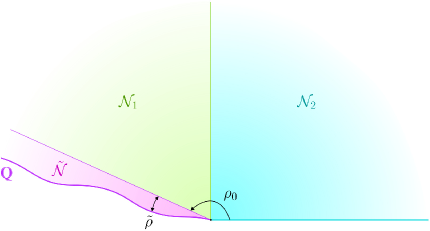
Figure 1: Schematics of the partial dimensional reduction of the AdS/BCFT setup with a fluctuating EOW brane $\mathbb{Q}$. Figure modified from Deng:2022yll .

Now performing this partial dimensional reduction for the bulk gravitational action given in eq. 1 for the wedge region $\mathcal{N}_{1}+\mathcal{\tilde{N}}$, one may obtain the action for the $2d$ effective theory as follows Deng:2022yll

$$I_{2d}=\frac{\rho_{0}}{16\pi G_{N}}\int_{\mathbb{Q}}\text{d}^{2}y\sqrt{-g^{(2)}}R^{(2)}+\frac{\rho_{0}}{16\pi G_{N}}\int_{\mathbb{Q}}\text{d}^{2}y\sqrt{-g^{(2)}}\frac{\tilde{\rho}}{\rho_{0}}\left(R^{(2)}+\frac{2}{L^{2}\cosh^{2}\big{(}\frac{\rho_{0}}{L}\big{)}}\right)+\ldots\,,$$ (7)

where $g_{ab}^{(2)}$ describes the AdS₂ metric with the length scale $L\cosh\big{(}\frac{\rho_{0}}{L}\big{)}$, $R^{(2)}$ is the scalar curvature corresponding to $g_{ab}^{(2)}$ and ellipsis denote $\mathcal{O}\left({\tilde{\rho}^{2}}/{\rho_{0}^{2}}\right)$ terms in the perturbative expansion. The $3d$ Newton’s constant $G_{N}$ is related to that in the $2d$ effective theory $G_{N}^{(2)}$ as follows Deng:2020ent ; Suzuki:2022xwv

$$\frac{1}{G_{N}^{(2)}}=\frac{\rho_{0}}{G_{N}}\,.$$ (8)

It should be noted here that in eq. 7, the tension of the EOW brane is considered to be the same as in eq. 5 as the fluctuation (6) only changes the tension up to $\mathcal{O}\big{(}\frac{\tilde{\rho}^{3}}{\rho_{0}^{3}}\big{)}$. Remarkably, eq. 7 describes the JT gravity action modulo certain boundary terms on identification of $\frac{\tilde{\rho}}{\rho_{0}}$ with the dilaton field. This provides us with a mechanism for obtaining JT gravity as a $2d$ effective theory through the partial dimensional reduction of an AdS₃ geometry with a fluctuating EOW brane.

2.2 Interface CFT

In this subsection, we review a class of interface CFT₂s (ICFT₂s) introduced in Anous:2022wqh . Their construction involves two CFT₂s defined on half lines coupled through a quantum dot. The bulk dual for such a theory is described by two locally AdS₃ geometries separated by a permeable EOW brane. The two CFT₂s located at the asymptotic boundary of the AdS₃ geometries are labelled as CFT${}^{\text{I}}$ and CFT${}^{\text{II}}$ with central charges $c_{\text{I}}$ and $c_{\text{II}}$ respectively, and the corresponding dual bulk locally AdS₃ geometries are labelled as AdS${}^{\text{I}}$ and AdS${}^{\text{II}}$ with length scales $L_{\text{I}}$ and $L_{\text{II}}$ respectively. In the semi-classical approximation, there is also an intermediate $2d$ effective perspective to describe this configuration, which may be obtained by integrating out bulk degrees of freedom. This results in the brane being characterized by a weakly gravitating system coupled to the original CFT${}^{\text{I,II}}$s. This $2d$ effective perspective will be discussed in detail in section 3 in the context of the JT gravity on the EOW brane.

The action for the dual bulk geometry describing the above configuration is given by Anous:2022wqh

$$I =\frac{1}{16\pi G_{N}}\left[\int_{\mathcal{B}_{\text{I}}}\text{d}^{3}x\sqrt{-g_{\text{I}}}\left(R_{\text{I}}+\frac{2}{L_{\text{I}}^{2}}\right)+\int_{\mathcal{B}_{\text{II}}}\text{d}^{3}x\sqrt{-g_{\text{II}}}\left(R_{\text{II}}+\frac{2}{L_{\text{II}}^{2}}\right)\right]$$ (9)

$$~{}+\frac{1}{8\pi G_{N}}\left[\int_{\Sigma}\text{d}^{2}y\sqrt{-h}(K_{\text{I}}-K_{\text{II}})-2T\int_{\Sigma}\text{d}^{2}y\sqrt{-h}\right]\,,$$

where $h_{ab}$ is the induced metric and $T$ is the tension of the EOW brane $\Sigma$. The relative minus sign between the two extrinsic curvatures $K_{\text{I,II}}$ is due to the fact that the outward normal is always taken to be pointing from the AdS${}^{\text{I}}$ to the AdS${}^{\text{II}}$ geometry. The properties of the EOW brane is fixed by requiring it to satisfy certain junction conditions. The first of these demands that the induced metric $h_{ab}$ on the brane be the same as viewed from either of the two AdS${}_{3}^{\text{I,II}}$ geometries. The second is the Israel junction condition for the brane with the two AdS${}_{3}^{\text{I,II}}$ geometries on either side which may be expressed as Anous:2022wqh

$$\big{(}K_{\text{I},ab}-K_{\text{II},ab}\big{)}-h_{ab}\big{(}K_{\text{I}}-K_{\text{II}}\big{)}=-T\,h_{ab}\,.$$ (10)

Solving these junction conditions will require us to specify the coordinate system describing the $3d$ geometry. To this end, the AdS₂ foliation of the AdS₃ geometry is chosen again on each patch of the spacetime $\mathcal{B}_{\text{I,II}}$ as follows

$$\text{d}s_{\mathcal{B}_{k}}^{2} =\text{d}\rho_{k}^{2}+L_{k}^{2}\cosh^{2}\left(\frac{\rho_{k}}{L_{k}}\right)\tilde{h}_{ab}\,\text{d}y^{a}\text{d}y^{b}$$ (12)

$$\equiv\text{d}\rho_{k}^{2}+L_{k}^{2}\cosh^{2}\left(\frac{\rho_{k}}{L_{k}}\right)\frac{-\text{d}t_{k}^{2}+\text{d}y_{k}^{2}}{y_{k}^{2}}\,,\quad\quad k=\text{I,II}\,.$$

Here $\tilde{h}_{ab}$ describes the usual Poincaré AdS₂ metric with unit radius. In these coordinates, the EOW brane is considered to be located at $\rho_{k}=\rho_{k}^{0}$ for $k=\text{I,II}$. The first junction condition thus implies the identification of $y_{k}$ and $t_{k}$ for both the coordinate patches. Additionally it also enforces the two AdS₂ radii to be the same i.e.,

$$L_{\text{I}}^{2}\cosh^{2}\left(\frac{\rho_{\text{I}}^{0}}{L_{\text{I}}}\right)=L_{\text{II}}^{2}\cosh^{2}\left(\frac{\rho_{\text{II}}^{0}}{L_{\text{II}}}\right)\,.$$ (13)

The solution to the second junction condition (10) fixes the position of the EOW brane as follows Anous:2022wqh

$$\tanh\left(\frac{\rho^{0}_{\text{I}}}{L_{\text{I}}}\right)=\frac{L_{\text{I}}}{2T}\left(T^{2}+\frac{1}{L_{\text{I}}^{2}}-\frac{1}{L_{\text{II}}^{2}}\right)\,,\qquad\tanh\left(\frac{\rho^{0}_{\text{II}}}{L_{\text{II}}}\right)=\frac{L_{\text{II}}}{2T}\left(T^{2}-\frac{1}{L_{\text{I}}^{2}}+\frac{1}{L_{\text{II}}^{2}}\right)\,.$$ (14)

Notice from the above that the tension $T$ of the brane has an upper as well as a lower bound. In the large tension limit described by

$$T\to T_{\text{max}}=\frac{1}{L_{\text{I}}}+\frac{1}{L_{\text{II}}}\,,$$ (15)

the EOW brane approaches the extended asymptotic boundary of both the AdS_k patches. In this limit, integrating out the bulk degrees of freedom on either side results in the two CFT₂s interacting through the weakly gravitating brane. This is the intermediate $2d$ effective scenario mentioned earlier which will be discussed in detail in the following section in the context of the JT gravity on the EOW brane.

3 Realising JT gravity at the interface of two spacetimes

In this section, we employ a combination of a partial Randall-Sundrum reduction and the usual AdS/CFT correspondence Deng:2022yll ; Deng:2020ent ; Chu:2021gdb ; Shao:2022gpg ; Li:2021dmf ; Basu:2022reu to the AdS/ICFT setup described in the preceding subsection, while allowing for small transverse fluctuations of the EOW brane $\Sigma$. This procedure results in a two dimensional effective theory comprising of the JT gravity on the EOW brane $\Sigma$ coupled to two non-gravitating bath CFT₂s. The gravity theory on the brane is obtained by integrating out the bulk AdS₃ geometry near the brane and may be thought of as the “bulk dual” of the interface degrees of freedom. On introducing the transverse fluctuations the locations of the EOW brane is described as follows

$$\Sigma~{}:~{} \rho_{\text{I}}=\rho^{0}_{\text{I}}-\tilde{\rho}_{\text{I}}(y)$$

$$\rho_{\text{II}}=\rho^{0}_{\text{II}}+\tilde{\rho}_{\text{II}}(y)\,.$$ (16)

The schematics of the setup is depicted in fig. 2. In the above equation, $\tilde{\rho}_{k}(y)\ll\rho^{0}_{k}$ are the small transverse fluctuations away from the brane angle $\rho^{0}_{k}$. Note that the fluctuation modes are functions of the braneworld coordinates $y$ and are treated as fields on the braneworld, as described in Geng:2022tfc ; Deng:2022yll . As depicted in fig. 2, we may divide the two AdS₃ geometries on either side of the EOW brane, into the wedges $W_{k}^{(1)}$ and $W_{k}^{(2)}$. With the fluctuations of the brane turned on, the wedge $W_{\text{II}}^{(1)}$ is extended further to include the small wedge region $\tilde{W}$ which is excised out of the wedge region $W_{\text{I}}^{(1)}$. Note that, in this setup the AdS₃ spacetimes on either sides of the brane are composed of several wedges as follows

$$\mathcal{B}_{\text{I}} =W_{\text{I}}^{(1)}+W_{\text{I}}^{(2)}-\tilde{W}\,,$$

$$\mathcal{B}_{\text{II}} =W_{\text{II}}^{(1)}+W_{\text{II}}^{(2)}+\tilde{W}\,.$$

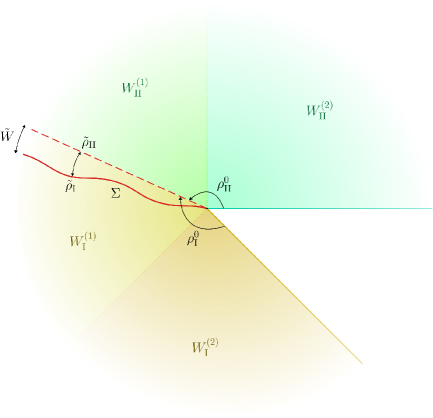
Figure 2: Schematics of the partial dimensional reduction of the AdS/ICFT setup with a fluctuating EOW brane $\Sigma$.

We now employ the partial dimensional reduction in the wedge regions $W_{\text{I}}^{(1)}-\tilde{W}$ in the AdS${}_{3}^{\text{I}}$ and $W_{\text{II}}^{(1)}+\tilde{W}$ in the AdS${}_{3}^{\text{II}}$ geometries by integrate out the bulk AdS₃ degrees of freedom in the $\rho_{\text{I,II}}$ direction(s). On the other hand, in the wedges $W_{k}^{(2)}$, we utilize the standard AdS₃/CFT₂ correspondence which leads to flat non-gravitating CFT₂s on the half lines stretching out from the interface. It is important to note here that in order to perform a perturbative analysis in $(\tilde{\rho}_{k}/\rho_{k}^{0})$, it is required to keep $\rho_{k}^{0}$ large. This restricts us in the large tension regime $T\to T_{\text{max}}$ of the AdS/ICFT setup as advocated in Anous:2022wqh . In this limit, the EOW brane $\Sigma$ is pushed towards the asymptotic boundaries of each AdS₃ geometry and hence the AdS₃ isometries are reminiscent of the conformal transformations on the brane. Therefore, it is natural to expect a gravitational theory coupled to the two bath CFT₂s to emerge in the lower dimensional effective description obtained from the partial dimensional reduction. In the following, we investigate the nature of this gravitational theory by explicitly integrating out the bulk AdS₃ geometries.

The three-dimensional bulk Ricci scalars are related to the $2d$ Ricci scalar $R^{(2)}$ on the brane $\Sigma$ as follows

$$\sqrt{-g_{k}}R_{k}=\sqrt{-g^{(2)}}\left[R^{(2)}-\frac{2\left(3\cosh^{2}\left(\frac{\rho_{k}}{L_{k}}\right)-1\right)}{L_{k}^{2}\cosh^{2}\left(\frac{\rho_{k}^{0}}{L_{k}}\right)}\right]\,,$$ (17)

where we have utilized the metric in eq. 12 with

$$g^{(2)}_{ab}=L_{k}^{2}\cosh^{2}\left(\frac{\rho_{k}}{L_{k}}\right)\tilde{h}_{ab}\,.$$ (18)

Integrating the $3d$ bulk Einstein-Hilbert actions (cf. eq. 9) of the AdS${}_{3}^{\text{I,II}}$ regions inside the wedges $W_{\text{I}}^{(1)}-\tilde{W}$ and $W_{\text{II}}^{(1)}+\tilde{W}$ leads to

$$\frac{1}{16\pi G_{N}}\int_{W_{\text{I}}^{(1)}-\tilde{W}}\text{d}^{3}x\sqrt{-g_{\text{I}}}\left(R_{\text{I}}+\frac{2}{L_{\text{I}}^{2}}\right)+\frac{1}{16\pi G_{N}}\int_{W_{\text{II}}^{(1)}+\tilde{W}}\text{d}^{3}x\sqrt{-g_{\text{II}}}\left(R_{\text{II}}+\frac{2}{L_{\text{II}}^{2}}\right)$$

$$=\frac{1}{16\pi G_{N}}\int_{\Sigma}\text{d}^{2}y\sqrt{-g^{(2)}}\left[\left(\rho^{0}_{\text{I}}-\tilde{\rho}_{\text{I}}(y)\right)R^{(2)}-\frac{\sinh\left(\frac{2\rho^{0}_{\text{I}}-2\tilde{\rho}_{\text{I}}(y)}{L_{\text{I}}}\right)}{L_{\text{I}}\cosh^{2}\left(\frac{\rho_{\text{I}}^{0}}{L_{\text{I}}}\right)}\right]$$

$$\quad\quad\quad\quad+\frac{1}{16\pi G_{N}}\int_{\Sigma}\text{d}^{2}y\sqrt{-g^{(2)}}\left[\left(\rho^{0}_{\text{II}}+\tilde{\rho}_{\text{II}}(y)\right)R^{(2)}-\frac{\sinh\left(\frac{2\rho^{0}_{\text{II}}+2\tilde{\rho}_{\text{II}}(y)}{L_{\text{II}}}\right)}{L_{\text{II}}\cosh^{2}\left(\frac{\rho_{\text{II}}^{0}}{L_{\text{II}}}\right)}\right]\,.$$ (19)

Next, we focus on the Gibbons-Hawking boundary terms and the tension term in eq. 9. The extrinsic curvatures $K_{\text{I,II}}$ may be computed using the outward normal vector pointing to $\text{I}\to\text{II}$ as follows

$$K_{\text{I},ab}=\frac{1}{L_{\text{I}}}\tanh\left[\frac{\rho^{0}_{\text{I}}-\tilde{\rho}_{\text{I}}(y)}{L_{\text{I}}}\right]\,h_{ab}~{}~{},~{}~{}K_{\text{II},ab}=-\frac{1}{L_{\text{II}}}\tanh\left[\frac{\rho^{0}_{\text{II}}+\tilde{\rho}_{\text{II}}(y)}{L_{\text{II}}}\right]\,h_{ab}\,,$$ (20)

where $h_{ab}$ is the induced metric on the brane

$$h_{ab}=L_{k}^{2}\cosh^{2}\left(\frac{\rho_{k}}{L_{k}}\right)\tilde{h}_{ab}\,,$$ (21)

and $\tilde{h}_{ab}$ is as defined in eq. 12. We keep the tension of the fluctuating brane constant as given in eq. 14, perturbatively in $\tilde{\rho}_{k}$. This may be interpreted as the tension of the brane remaining intact under small transverse fluctuations. Hence, the Gibbons-Hawking boundary term together with the brane tension term leads to

$$\frac{1}{8\pi G_{N}}\left[\int_{\Sigma}\text{d}^{2}y\sqrt{-h}(K_{\text{I}}-K_{\text{II}})-2T\int_{\Sigma}\text{d}^{2}y\sqrt{-h}\right]$$

$$=\frac{1}{8\pi G_{N}}\int_{\Sigma}\text{d}^{2}y\sqrt{-g^{(2)}}\left[\frac{\sinh\left(\frac{2\rho^{0}_{\text{I}}-2\tilde{\rho}_{\text{I}}(y)}{L_{\text{II}}}\right)}{L_{\text{I}}\cosh^{2}\left(\frac{\rho_{\text{I}}^{0}}{L_{\text{I}}}\right)}-\frac{\tanh\left(\frac{\rho_{\text{I}}^{0}}{L_{\text{I}}}\right)\cosh^{2}\left(\frac{\rho^{0}_{\text{I}}-\tilde{\rho}_{\text{I}}(y)}{L_{\text{II}}}\right)}{L_{\text{I}}\cosh^{2}\left(\frac{\rho_{\text{I}}^{0}}{L_{\text{I}}}\right)}\right]$$

$$\qquad\qquad+\frac{1}{8\pi G_{N}}\int_{\Sigma}\text{d}^{2}y\sqrt{-g^{(2)}}\left[\frac{\sinh\left(\frac{2\rho^{0}_{\text{II}}+2\tilde{\rho}_{\text{II}}(y)}{L_{\text{II}}}\right)}{L_{\text{II}}\cosh^{2}\left(\frac{\rho_{\text{II}}^{0}}{L_{\text{II}}}\right)}-\frac{\tanh\left(\frac{\rho_{\text{II}}^{0}}{L_{\text{II}}}\right)\cosh^{2}\left(\frac{\rho^{0}_{\text{II}}+\tilde{\rho}_{\text{II}}(y)}{L_{\text{II}}}\right)}{L_{\text{II}}\cosh^{2}\left(\frac{\rho_{\text{II}}^{0}}{L_{\text{II}}}\right)}\right]\,.$$ (22)

Adding the contributions from eqs. 19 and 22 and expanding perturbatively in small $\left(\tilde{\rho}_{k}/\rho_{k}^{0}\right)$ the total bulk action for the lower dimensional effective gravitational theory on the brane $\Sigma$, upon partial dimensional reduction on the wedges $W_{\text{I}}^{(1)}-\tilde{W}$ and $W_{\text{II}}^{(1)}+\tilde{W}$, becomes

$$I_{\text{total}}=\frac{\rho^{0}_{\text{I}}+\rho^{0}_{\text{II}}}{16\pi G_{N}}\int_{\Sigma}\text{d}^{2}y\sqrt{-g^{(2)}} R^{(2)}-\frac{1}{16\pi G_{N}}\int_{\Sigma}\text{d}^{2}y\sqrt{-g^{(2)}}\,\tilde{\rho}_{\text{I}}(y)\Bigg{[}R^{(2)}+\frac{2}{L_{\text{I}}^{2}\cosh^{2}\left(\frac{\rho_{\text{I}}^{0}}{L_{\text{I}}}\right)}\Bigg{]}$$ (23)

$$\quad+\frac{1}{16\pi G_{N}}\int_{\Sigma}\text{d}^{2}y\sqrt{-g^{(2)}}\,\tilde{\rho}_{\text{II}}(y)\Bigg{[}R^{(2)}+\frac{2}{L_{\text{II}}^{2}\cosh^{2}\left(\frac{\rho_{\text{II}}^{0}}{L_{\text{II}}}\right)}\Bigg{]}\,,$$

where we have neglected terms of order $({\tilde{\rho}_{k}}/{\rho_{k}^{0}})^{2}$. Utilizing eq. 13, the above action may be rewritten in the instructive form

$$I_{\text{total}}=\frac{1}{16\pi G_{N}^{(2)}}\left[\int_{\Sigma}\text{d}^{2}y\sqrt{-g^{(2)}}\,R^{(2)}+\int_{\Sigma}\text{d}^{2}y\sqrt{-g^{(2)}}\,\Phi(y)\left(R^{(2)}+\frac{2}{\ell_{\text{eff}}^{2}}\right)\right]\,,$$ (24)

where we have defined the two dimensional Newton’s constant $G_{N}^{(2)}$ and the curvature scale $\ell_{\text{eff}}$ on the brane $\Sigma$ as follows

$$\frac{1}{G_{N}^{(2)}}=\frac{\rho^{0}_{\text{I}}+\rho^{0}_{\text{II}}}{G_{N}}~{}~{},~{}~{}\ell_{\text{eff}}=L_{\text{I}}\cosh\left(\frac{\rho_{\text{I}}^{0}}{L_{\text{I}}}\right)=L_{\text{II}}\cosh\left(\frac{\rho_{\text{II}}^{0}}{L_{\text{II}}}\right)\,.$$ (25)

Furthermore, in eq. 24, we have identified the dilaton field $\Phi(y)$ on the brane with the fluctuations of the brane angles $\tilde{\rho}_{k}(y)$ as follows

$$\Phi(y)=\frac{\tilde{\rho}_{\text{II}}(y)-\tilde{\rho}_{\text{I}}(y)}{\rho^{0}_{\text{I}}+\rho^{0}_{\text{II}}}\,.$$ (26)

With these identifications, the $2d$ bulk action in eq. 24 precisely takes the form of the action for JT gravity modulo certain boundary terms, with the topological part of the dilaton field $\Phi_{0}$ set equal to unity. Furthermore, variation of the action with respect to the dilaton field $\Phi(y)$ leads to the Ricci scalar as

$$R^{(2)}=-\frac{2}{\ell_{\text{eff}}^{2}}=-\frac{2}{L_{k}^{2}\cosh^{2}\left(\frac{\rho_{k}^{0}}{L_{k}}\right)}~{}~{},~{}~{}k=\text{I,II}$$ (27)

which correctly conforms to the fact that the brane is situated at a particular AdS₂ slice as seen from either of the bulk AdS₃ spacetimes.

At this point we recall that, in the limit of large $\rho_{k}^{0}$ the EOW brane $\Sigma$ is pushed towards the asymptotic boundary of each AdS₃ spacetime. As described in Chen:2020uac ; Fallows:2021sge , in this limit one obtains a non-local action Skenderis:1999nb instead of the first term in eq. 24 as follows

$$I_{\text{non-local}}=\sum_{k=\text{I},\text{II}}\frac{L_{k}}{32\pi G_{N}} \int_{\Sigma}\text{d}^{2}y\sqrt{-\tilde{h}}\,\left[R^{(2)}-R^{(2)}\log\left(-\frac{L^{2}_{k}}{2}R^{(2)}\right)\right]\,.$$ (28)

By introducing two auxiliary scalar fields $\varphi_{k}~{}(k=\text{I\,,\,II})$, the above mentioned non-local action may be rewritten in a local form in terms of the usual Polyakov action as discussed in Anous:2022wqh

$$I_{\text{Poly}}=\sum_{k=\text{I},\text{II}} \frac{L_{k}}{32\pi G_{N}}\int_{\Sigma}\text{d}^{2}y\sqrt{-\tilde{h}}\left[-\frac{1}{2}\tilde{h}^{ab}\nabla_{a}\varphi_{k}\nabla_{b}\varphi_{k}+\varphi_{k}R^{(2)}-\frac{2}{L_{k}^{2}}\,e^{-\varphi_{k}}\right]\,.$$ (29)

We may interpret the above Polyakov action as two CFT₂s with central charges $c_{\text{I}}$ and $c_{\text{II}}$ located on the AdS₂ brane Anous:2022wqh . The JT gravity on the brane is coupled to these CFT₂s which are also identical to the two bath CFT₂s on the two half lines obtained via the standard AdS₃/CFT₂ dictionary on the bulk wedges $W_{k}^{(2)}$. In other words, we have two CFT₂s defined on the whole real line. In half of the lines the CFT₂s live on a curved AdS₂ manifold that is the brane, and are coupled to each other via the JT gravity on this curved manifold. In the other half, the CFT₂s live on two flat non-gravitating manifolds and hence are decoupled. The schematics of this $2d$ effective scenario is sketched in fig. 3.

Figure 3: Schematics of the $2d$ effective theory comprised of JT gravity coupled to two flat CFT₂ baths.

To illustrate the emergence of the two CFT₂s on the brane via the Polyakov action in eq. 29, we note that the zero-dimensional analogue of the transverse area of a codimension two surface $\mathcal{X}$ on the brane is given, for the action eq. 29, by Fallows:2021sge

$$\mathcal{A}(\mathcal{X})=\frac{\Phi(\mathcal{X})}{4G_{N}^{(2)}}+\frac{1}{8G_{N}}\sum_{k=\text{I},\text{II}}L_{k}\,\varphi_{k}(\mathcal{X})\,.$$ (30)

For the brane $\Sigma$ situated at the AdS₂ slice described by eq. 27, the auxiliary scalar fields $\varphi_{k}$ may be obtained as Chen:2020uac

$$\varphi_{k}=\log\left[-\frac{2}{L_{k}^{2}R^{(2)}}\right]=2\,\log\left[\cosh\left(\frac{\rho_{k}^{0}}{L_{k}}\right)\right]\,,$$ (31)

and hence the area term in eq. 30 is given by

$$\mathcal{A}(\mathcal{X})=\frac{\Phi(\mathcal{X})}{4G_{N}^{(2)}}+\frac{c_{\text{I}}}{6}\log\left(\frac{1}{\cos\psi_{\text{I}}}\right)+\frac{c_{\text{II}}}{6}\log\left(\frac{1}{\cos\psi_{\text{II}}}\right)\,,$$ (32)

where we have utilized eq. 11.

To conclude we have obtained an effective intermediate braneworld description involving the JT gravity on a dynamical manifold coupled with two bath CFT₂s through a dimensional reduction of a $3d$ bulk which could be understood as a doubly holographic description for the effective $2d$ theory. Recall that this $3d$ bulk has a holographic dual described by an interface CFT where the interface degrees of freedom may be interpreted as an SYK quantum dot.

3.1 Generalized entropy

Consider a QFT coupled to a gravitational theory on an hybrid manifold $\mathcal{M}=\Sigma\,\cup\mathcal{M}^{\text{I}}\cup\mathcal{M}^{\text{II}}$, where $\Sigma$ corresponds to the dynamical EOW brane in the doubly holographic $3d$ description which smoothly joins with the two non-gravitating flat baths $\mathcal{M}^{\text{I,II}}$. Transparent boundary conditions are imposed at the common boundary of $\Sigma$ and $\mathcal{M}^{\text{I,II}}$ such that the quantum matter fields freely propagate across this boundary. The generalized Rényi entropy for a subsystem $A$ on this hybrid manifold could be obtained through a path integral on the replicated geometry $\mathcal{M}_{n}=\Sigma_{n}\cup\mathcal{M}_{n}^{\text{I}}\cup\mathcal{M}_{n}^{\text{II}}$ with branch cuts at the endpoints of $A$ as follows

$$(1-n)S^{(n)}_{\text{gen}}(A)=\log\text{Tr}\boldsymbol{\rho}^{n}_{A}=\log\frac{\mathbb{Z}\left[\mathcal{M}_{n}\right]}{\left(\mathbb{Z}\left[\mathcal{M}_{1}\right]\right)^{n}}\,,$$ (33)

where $\boldsymbol{\rho}_{A}$ is the reduced density matrix for $A$ in the full quantum theory and $\mathbb{Z}[\mathcal{M}_{n}]$ corresponds to the partition function of the manifold $\mathcal{M}_{n}$. Under the semiclassical approximation, the gravitational path integral could be approximated near its saddle point to obtain the partition function on the replicated manifold $\mathcal{M}_{n}$ as follows

$$\mathbf{Z}\left[\mathcal{M}_{n}\right]\approx e^{-\text{I}_{\text{grav}}\left[\Sigma_{n}\right]}\,\mathbf{Z}_{\text{mat}}\left[\mathcal{M}_{n}\right]\,,$$ (34)

where $\mathbf{Z}_{\text{mat}}\left[\mathcal{M}_{n}\right]$ in the matter partition function on the entire replicated hybrid manifold $\mathcal{M}_{n}$ while $\text{I}_{\text{grav}}\left[\Sigma_{n}\right]$ is the classical gravitational action on the dynamical manifold $\Sigma_{n}$.

If the replica symmetry for the bulk saddle point configuration in the semiclassical approximation remains intact, the orbifold $\tilde{\mathcal{M}}_{n}\equiv\mathcal{M}_{n}/\mathbb{Z}_{n}$ obtained by quotienting via the replica symmetry $\mathbb{Z}_{n}$ contains conical defects with deficit angle $\Delta\phi_{n}=2\pi(1-1/n)$ along the replica fixed points in the bulk geometry. This is the so-called replica wormhole saddle discussed in the literature Almheiri:2019hni ; Almheiri:2019qdq ; Almheiri:2019yqk ; Penington:2019kki . The region enclosed between these conical singularities in the bulk constitute the island $\text{Is}(A)$ for the subsystem $A$.

In the semiclassical description, the (normalized) matter partition function $\mathbf{Z}_{\text{mat}}$ computes the effective Rényi entropy of the quantum matter fields inside the entanglement wedge of $A\cup\text{Is}(A)$ as follows

$$\frac{\mathbf{Z}_{\text{mat}}[\mathcal{M}_{n}]}{\big{(}\mathbf{Z}_{\text{mat}}[\mathcal{M}_{1}]\big{)}^{n}}=\text{e}^{(1-n)\log\text{Tr}\rho_{A\cup\text{Is}(A)}^{n}}\,,$$ (35)

where $\rho_{A\cup\text{Is}(A)}$ is the effective reduced density matrix in the semiclassical description.

Unlike the earlier works where JT gravity was coupled to a single radiation bath, in the current scenario, the presence of two baths modifies the structure of the dominant replica wormhole saddle to provide two independent mechanisms for the origin of the island region in the semiclassical description:

• For a subsystem $A=A^{\text{I}}\cup A^{\text{II}}$ with $A^{\text{I,II}}\subset\mathcal{M}^{\text{I,II}}$ in the radiation baths, both $A^{\text{I}}$ and $A^{\text{II}}$ are responsible for the conical singularities appearing in the gravitating manifold $\Sigma$. In this situation, the corresponding island region $\text{Is}(A)$ manifested in $\Sigma$ depends upon the degrees of freedom for both the CFT baths. In other words, if we denote the islands corresponding to the individual baths as $\text{Is}^{\text{I,II}}(A)$, for the present configuration we have $\text{Is}^{\text{I}}(A)=\text{Is}^{\text{II}}(A)\equiv\text{Is}(A)$ and the density matrix in the effective theory factorizes in the following way

  $$\rho_{A\cup\text{Is}(A)}\sim\rho_{A^{\text{I}}\cup\text{Is}(A)}\otimes\rho_{A^{\text{II}}\cup\text{Is}(A)}\,.$$ (36)

  This could also be understood through the doubly holographic formalism where we have gravitational regions on either sides of the fluctuating EOW brane. Recall that in the doubly holographic description, the island region in this scenario is described by the region on the EOW brane between the two RTs crossing from AdS${}^{\text{I}}$ to AdS${}^{\text{II}}$. For the present configuration the bulk RT surface homologous to the subsystem $A$ is composed of two geodesics connecting the endpoints of $A^{\text{I}}$ and $A^{\text{II}}$, each of which crosses the EOW brane only once as depicted in fig. 4(a). This corresponds to the conventional origin of the island region as described in Almheiri:2019qdq ; Almheiri:2019yqk .

• On the other hand, consider a subsystem $A$ residing entirely in the bath $\mathcal{M}^{\text{II}}$. If the central charge of the CFT${}^{\text{II}}$ is larger than that of the CFT${}^{\text{I}}$, depending upon the size of the subsystem $A$, conical singularities in the gravitating region $\Sigma$ may appear solely due to the presence of $A$ in the bath $\mathcal{M}^{\text{II}}$. Since the bulk region $\Sigma$ is common between the bath CFTs, the CFT${}^{\text{I}}$ degrees of freedom present in $\Sigma$ sense the same conical singularities and conceive an induced island which we denote by $\text{Is}^{(\text{I}\backslash\text{II})}(A)$ to indicate that we obtain an island region in CFT${}^{\text{I}}$ given some subsystem $A$ in CFT${}^{\text{II}}$. In this case, the density matrix in the effective theory reduces to

  $$\rho_{A\cup\text{Is}(A)}\sim\rho_{\text{Is}^{(\text{I}\backslash\text{II})}(A)}\otimes\rho_{A^{\text{II}}\cup\text{Is}(A)}\,.$$ (37)

  From the doubly holographic perspective, this corresponds to a double-crossing geodesic where the minimal curve penetrates into AdS${}^{\text{I}}$ and returns to AdS${}^{\text{II}}$ in order to satisfy the homology condition which is depicted in fig. 4(b). Note that such an island region is a novelty of the present model where a gravitational theory is coupled to two flat baths.

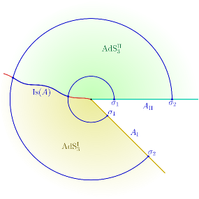
(a) Schematics of the bulk geodesic homologous to the subsystem $A=A_{\text{I}}\cup A_{\text{II}}$ described by a finite interval $A_{\text{I,II}}$ in dual CFT${}^{\text{I,II}}$.

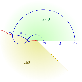
(b) Schematics of the (double-crossing) bulk geodesic homologous to the subsystem $A$ described by a finite interval [$\sigma_{1},\sigma_{2}$] in dual CFT${}^{\text{II}}$.

Figure 4: Two independent mechanisms for the origin of the island region $\text{Is}(A)$ in ICFTs.

Assuming that the backreactions from the conical defects are small, the replica wormhole saddle are still solutions to the Einstein’s equations. In such case, the classical gravitational action $\text{I}_{\text{grav}}[\Sigma_{n}]$ in eq. 34, for the replica wormhole saddle Almheiri:2019qdq ; Dong:2020uxp may be expressed for $n\sim 1$ as

$$\text{I}_{\text{grav}}\big{[}\Sigma_{n}\big{]}\approx n\,\text{I}_{\text{grav}}\big{[}\tilde{\Sigma}_{1}\big{]}+\frac{n-1}{4G_{N}^{(2)}}\mathcal{A}\big{(}\partial\text{Is}(A)\big{)}\,,$$ (38)

where $\tilde{\Sigma}_{n}\equiv\Sigma_{n}/\mathbb{Z}_{n}$ is the orbifold for the replicated bulk geometry $\Sigma_{n}$ and $\mathcal{A}\big{(}\partial\text{Is}(A)\big{)}$ is the area of the boundary of the island region $\text{Is}(A)$, namely the quantum extremal surface for the subsystem $A$. Utilizing eqs. 33, 34 and 38, we may now obtain the generalized entropy corresponding to the reduced density matrix $\boldsymbol{\rho}_{A}$ for the subsystem $A$ as follows

$$S_{\text{gen}}\left(\boldsymbol{\rho}_{A}\right) =\frac{\mathcal{A}\big{(}\partial\text{Is}(A)\big{)}}{4G_{N}^{(2)}}+S_{\text{eff}}\left(\rho_{A\cup\text{Is}(A)}\right)_{\mathcal{M}^{\text{I}}\cup\mathcal{M}^{\text{II}}\cup\Sigma}$$

$$=\frac{\mathcal{A}\big{(}\partial\text{Is}(A)\big{)}}{4G_{N}^{(2)}}+S_{\text{eff}}^{\text{I}}\left(\rho_{A^{\text{I}}\cup\text{Is}(A)}\right)_{\mathcal{M}^{\text{I}}\cup\Sigma}+S_{\text{eff}}^{\text{II}}\left(\rho_{A^{\text{II}}\cup\text{Is}(A)}\right)_{\mathcal{M}^{\text{II}}\cup\Sigma}\,,$$ (39)

for the conventional island. Note that the subscripts $\mathcal{M}^{\text{I,II}}\cup\Sigma$ denote that the reduced density matrices $\rho_{A^{\text{I,II}}\cup\text{Is}(A)}$ in the effective theory have support on corresponding manifolds. On the other hand, for the configuration where we observe the induced island, the generalized entropy modifies to

$$S_{\text{gen}}\left(\boldsymbol{\rho}_{A}\right)=\frac{\mathcal{A}\big{(}\partial\text{Is}(A)\big{)}}{4G_{N}^{(2)}}+S_{\text{eff}}^{\text{I}}\left(\rho_{\text{Is}^{(\text{I}\backslash\text{II})}(A)}\right)_{\Sigma}+S_{\text{eff}}^{\text{II}}\left(\rho_{A^{\text{II}}\cup\text{Is}(A)}\right)_{\mathcal{M}^{\text{II}}\cup\Sigma}\,.$$ (40)

Note that the area term in eqs. 39 and 40 for the generalized entropies are as given in eq. 32.

4 Islands in extremal JT black holes

In this section, we will compute the entanglement entropies of various subsystems at a zero temperature in the CFT${}_{2}^{\text{I}}$ and CFT${}_{2}^{\text{II}}$ baths in the braneworld setup discussed above. In particular, we will compute the entanglement entropy for the corresponding subsystems in the intermediate picture using the island formula. Subsequently, we will substantiate these field theory results from the bulk computation of the RT surfaces corresponding to the subsystem using double holography in the large tension limit in which the gravity on the brane is weakly coupled.

As described in Almheiri:2019hni ; Almheiri:2019qdq ; Almheiri:2019yqk , the dilaton profiles may be obtained from the equation of motion which arises from the JT action in eq. 24 by varying it with respect to the metric for the case of extremal black hole as follows

$$\text{d}s^{2}=\frac{4\,\text{d}\zeta_{k}\text{d}\overline{\zeta}_{k}}{\left(\zeta_{k}+\overline{\zeta}_{k}\right)^{2}}~{}~{},~{}~{}~{}~{}~{}~{}\Phi=\Phi_{0}-\frac{2\Phi_{r}}{\zeta_{k}+\overline{\zeta}_{k}}\,,$$ (41)

where $\zeta=x+it_{E}$ are the planar coordinates and $\Phi_{0}$ is the topological contribution to the dilaton given in eq. 32.

4.1 Semi-infinite subsystem

We consider the case where a subsystem $A$ is comprised of a semi-infinite interval in each bath CFT₂s as $A\equiv[\sigma_{1},\infty]_{\text{I}}\cup[\sigma_{2},\infty]_{\text{II}}$. We describe the computation of the entanglement entropy of the subsystem $A$ using the island prescription in the effective $2d$ description discussed in section 3.1. Later we utilize the Ryu-Takayanagi (RT) prescription Ryu:2006bv to compute the entanglement entropy of the corresponding interval in the doubly holographic framework.

Effective $2d$ description

For this configuration involving a semi-infinite subsystem, only the conventional island appears. Consider the QES to be located at $-a$ on the EOW brane. Note that both the CFT${}_{2}^{\text{I}}$ and CFT${}_{2}^{\text{II}}$ are located on the JT brane, thus as discussed in section 3.1, the conical singularity at the QES $-a$ is present in both CFT${}_{2}^{\text{I}}$ and CFT${}_{2}^{\text{II}}$. As can be inferred from eq. 41, the UV cutoff on the JT brane has position dependence as $\epsilon(-a)=a$. Hence, utilizing eq. 39, the generalized entanglement entropy for subsystem $A$ may be obtained as

$$S_{\text{gen}}=\frac{\Phi_{r}}{a}+\frac{c_{\text{I}}}{6}\log\left[\frac{1}{\cos\psi_{\text{I}}}\right]+\frac{c_{\text{II}}}{6}\log\left[\frac{1}{\cos\psi_{\text{II}}}\right]+\frac{c_{\text{I}}}{6}\log\bigg{[}\frac{\left(\sigma_{1}+a\right)^{2}}{\epsilon\,a}\bigg{]}+\frac{c_{\text{II}}}{6}\log\bigg{[}\frac{\left(\sigma_{2}+a\right)^{2}}{\epsilon\,a}\bigg{]}\,,$$ (42)

where we have used eq. 32 for the area of the quantum extremal surface located on the JT brane. The entanglement entropy may now be obtained through the extremization of the above generalized entropy over the position of the island surface. The extremization for arbitrary $\sigma_{1}$ and $\sigma_{2}$, however leads to complicated expressions. Thus for simplicity, we assume the symmetric case $\sigma_{1}=\sigma_{2}=\sigma$, for which the extremization equation is given by

$$\partial_{a}S_{\text{gen}}=0\quad\Rightarrow\quad\quad a\left(c_{\text{I}}+c_{\text{II}}\right)(a-\sigma)-6(a+\sigma)\Phi_{r}\ =0\,.$$ (43)

Finally, the location of the island region $a^{*}$ may be obtained from the above quadratic equation as follows

$$a^{*}=\frac{\left(c_{\text{I}}+c_{\text{II}}\right)\sigma+6\Phi_{r}+\sqrt{\big{(}\left(c_{\text{I}}+c_{\text{II}}\right)\sigma+6\Phi_{r}\big{)}^{2}+24\left(c_{\text{I}}+c_{\text{II}}\right)\sigma\Phi_{r}}}{2\left(c_{\text{I}}+c_{\text{II}}\right)}\,,$$ (44)

where we have disregarded the unphysical solution of the QES. The fine-grained entropy for the subsystem $A$ may finally be obtained by substituting the above extremal value in eq. 42. In order to compare this result with the doubly holographic computation in the following subsection, we need to consider the large tension limit of the JT brane for which the brane angles $\psi_{\text{I,II}}$ may be expanded as Anous:2022wqh

$$\psi_{\text{I}}=\frac{\pi}{2}-\frac{L_{\text{I}}}{L_{\text{I}}+L_{\text{II}}}\delta\,,\quad\,\quad\psi_{\text{II}}=\frac{\pi}{2}-\frac{L_{\text{II}}}{L_{\text{I}}+L_{\text{II}}}\delta\,,\qquad\quad\text{with }\delta\rightarrow 0\,,$$ (45)

where the finite but small $\delta$ describes the deviation of the JT brane from the extended conformal boundary of the AdS${}_{3}^{\text{I,II}}$.

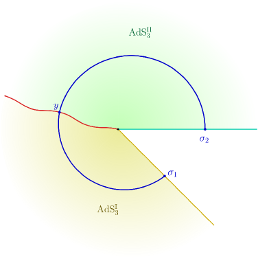
Figure 5: Schematics of the bulk geodesic homologous to the subsystem $A$ described by the union of two semi-infinite intervals in both CFT${}^{\text{I}}$ and CFT${}^{\text{II}}$.

Doubly holographic description

In this subsection, we substantiate the above island results in the effective field theory from a doubly holographic perspective. To this end, the metric described in eq. 12 may be mapped to the Poincaré AdS₃ geometry through the following coordinate transformations

$$z_{k}=y\cos\chi_{k}~{},\qquad x_{k}=y\sin\chi_{k}~{}.$$ (46)

The radial direction in the $xz$-plane in the Poincaré coordinates is described by the coordinate $y$. At the asymptotic boundary described by $\chi_{k}=\pm\pi/2$, $y$ now serves as a boundary coordinate. Furthermore, the length of a geodesic between points $(t,x,z)$ and $(t^{\prime},x^{\prime},z^{\prime})$ in the Poincaré coordinates, is obtained through

$${d}=L\,\cosh^{-1}\left[\frac{-(t-t^{\prime})^{2}+(x-x^{\prime})^{2}+z^{2}+z^{\prime 2}}{2z\,z^{\prime}}\right]~{}.$$ (47)

Note that for the present configuration, the RT surface homologous to subsystem $A$ consists of two semi-circular geodesic segments in each of the AdS${}_{3}^{\text{I,II}}$ geometries which are smoothly joined at the EOW brane as depicted in fig. 5. As a consequence of the Israel junction condition, we may choose the common point on the EOW brane to be parametrized by a single variable $y$. The total length of the RT surface may then be expressed as

$${d}= L_{\text{I}}\log\left[\frac{\left(\sigma_{1}+y\sin\psi_{\text{I}}\right){}^{2}+\left(y\cos\psi_{\text{I}}\right)^{2}}{\epsilon\,y\cos\psi_{\text{I}}}\right]+L_{\text{II}}\log\left[\frac{\left(\sigma_{2}+y\sin\psi_{\text{II}}\right)^{2}+\left(y\cos\psi_{\text{II}}\right)^{2}}{\epsilon\,y\cos\psi_{\text{II}}}\right]\,,$$ (48)

Subsequently, we perturb the EOW brane by introducing a small fluctuation in the brane angles $\psi_{\text{I,II}}$ as follows

$$\psi_{{k}}(y)\to\sin^{-1}\left[\tanh\left(\frac{\rho_{{k}}^{0}+(-1)^{k}\tilde{\rho}_{k}(y)}{L_{k}}\right)\right]~{},$$ (49)

where $\frac{\tilde{\rho}_{\text{{I,II}}}}{\rho_{\text{{I,II}}}^{0}}\ll 1$. Utilizing the above relation, eq. 48 reduces to

$${d} =L_{\text{I}}\log\left[\frac{2\sigma_{1}y\tanh\left(\frac{\rho_{\text{I}}^{0}}{L_{\text{I}}}\right)+\sigma_{1}^{2}+y^{2}}{\epsilon\,y\,\text{sech}\left(\frac{\rho_{\text{I}}^{0}}{L_{\text{I}}}\right)}\right]+L_{\text{II}}\log\left[\frac{2\sigma_{2}y\tanh\left(\frac{\rho_{\text{II}}^{0}}{L_{\text{II}}}\right)+\sigma_{2}^{2}+y^{2}}{\epsilon\,y\,\text{sech}\left(\frac{\rho_{\text{II}}^{0}}{L_{\text{II}}}\right)}\right]$$

$$-\frac{\tilde{\rho}_{\rm I}\left(\sigma_{1}^{2}\tanh\left(\frac{\rho_{\text{I}}^{0}}{L_{\text{I}}}\right)+y^{2}\tanh\left(\frac{\rho_{\text{I}}^{0}}{L_{\text{I}}}\right)+2\sigma_{1}y\right)}{2\sigma_{1}y\tanh\left(\frac{\rho_{\text{I}}^{0}}{L_{\text{I}}}\right)+\sigma_{1}^{2}+y^{2}}+\frac{\tilde{\rho}_{\rm II}\left(\sigma_{2}^{2}\tanh\left(\frac{\rho_{\text{II}}^{0}}{L_{\text{II}}}\right)+y^{2}\tanh\left(\frac{\rho_{\text{II}}^{0}}{L_{\text{II}}}\right)+2\sigma_{2}y\right)}{2\sigma_{2}y\tanh\left(\frac{\rho_{\text{II}}^{0}}{L_{\text{II}}}\right)+\sigma_{2}^{2}+y^{2}}~{}.$$ (50)

where we have considered terms up to the first order in $\tilde{\rho}_{\rm I,II}$. Note that, the perturbative parameters $\tilde{\rho}_{\rm I,II}$ are functions of the island location $y$. Therefore, in the perturbative terms of the above expression, we replace $y$ with its zeroth order solution in $\tilde{\rho}_{\text{I,II}}$ such that the geodesic length in section 4 contains terms truly upto the first order in $\tilde{\rho}_{\text{I,II}}$. Subsequently, on identifying the dilaton as given in eq. 26, the candidate entanglement entropy may be obtained as follows

$$S_{\rm single}(\sigma,y)=\frac{\Phi_{r}}{y}+\frac{L_{\text{I}}}{4G_{N}}\log\left[\frac{\sigma^{2}+y^{2}+2\sigma\,y\sin\psi_{\rm I}}{\epsilon\,y\cos\psi_{\rm I}}\right]+\frac{L_{\text{II}}}{4G_{N}}\log\left[\frac{\sigma^{2}+y^{2}+2\sigma\,y\sin\psi_{\rm II}}{\epsilon\,y\cos\psi_{\rm II}}\right],$$ (51)

where we have considered $\sigma_{1}=\sigma_{2}=\sigma$ for simplicity. Now, to obtain the holographic entanglement entropy, we extremize the above with respect to $y$ to obtain

$$L_{\text{II}}\,y(y-\sigma)(y+\sigma) \left[\left(y^{2}+\sigma^{2}\right)\left(\cos\psi_{\text{I}}\,\sec\psi_{\text{II}}+1\right)+2\sigma\,y\sin(\psi_{\text{I}}+\psi_{\text{II}})\sec\psi_{\text{II}}\right]$$

$$-4G_{N}\Phi_{r}\left(y^{2}+\sigma^{2}+2\sigma\,y\sin\psi_{\text{I}}\right)\left(y^{2}+\sigma^{2}+2\sigma\,y\sin\psi_{\text{II}}\right)=0~{}.$$ (52)

The entanglement entropy for the semi-infinite subsystem in question may be obtained by substituting the physical solution for $y$ in eq. 51. Finally, in the large tension limit described in eq. 45, this matches exactly with the corresponding entanglement entropy computed in the effective $2d$ theory on utilization of the Brown-Henneaux formula $c_{\text{I,II}}=\frac{3{L}_{\text{I,II}}}{2G_{N}}$ Brown:1986nw .

4.2 Finite subsystem

In this subsection, we obtain the entanglement entropy for a finite sized subsystem $A\equiv[\sigma_{1},\sigma_{2}]_{\text{I}}\cup[\sigma_{1},\sigma_{2}]_{\text{II}}$ located in the baths CFT${}_{2}^{\text{I}}$ and CFT${}_{2}^{\text{II}}$. Here, we observe three non-trivial phases for the generalized entanglement entropy depending upon the sizes of the subsystem $A$ as depicted in figs. 8, 7 and 6. In this context, we first utilize the effective $2d$ prescription to compute the generalized entanglement entropy for the corresponding subsystem in these scenarios. Subsequently, we provide a doubly holographic characterization of the entanglement entropy for the three cases using the RT prescription which substantiates the corresponding field theory results.

4.2.1 Phase - I

Effective $2d$ description

We begin with the computation of the generalized entanglement entropy for the phase where the intervals $[\sigma_{1},\sigma_{2}]_{\text{I}}$ and $[\sigma_{1},\sigma_{2}]_{\text{II}}$ are small such that no island region is observed as depicted in fig. 6. For this configuration the area term in generalized entropy vanishes and the expression for the entanglement entropy may trivially be obtained to be

$$S_{A}= \frac{(c_{\text{I}}+c_{\text{II}})}{3}\log\left[\frac{\sigma_{2}-\sigma_{1}}{\epsilon}\right]\,.$$ (53)

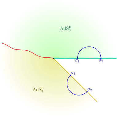
Figure 6: Schematics of the phase-I for the bulk geodesic homologous to the subsystem $A$ described by a finite interval $[\sigma_{1},\sigma_{2}]_{\text{I,II}}$ in dual CFT${}^{\text{I,II}}$.

Doubly holographic description

From the doubly holographic perspective, it may be observed that the RT surfaces for the intervals $[\sigma_{1},\sigma_{2}]_{\text{I,II}}$ in CFT${}_{2}^{\text{I,II}}$ are described by the usual dome-shaped geodesics each in the dual bulk AdS${}_{3}^{\text{I,II}}$ geometries as depicted in fig. 6. The entanglement entropy for this configuration may then be obtained to be

$$S_{\rm dome}=\frac{(L_{\text{I}}+L_{\text{II}})}{4G_{N}}\log\left[\frac{\sigma_{2}-\sigma_{1}}{\epsilon}\right]\,,$$ (54)

which matches identically with the corresponding expression obtained in the effective $2d$ description in eq. 53 through the utilization of the Brown-Henneaux formula.

4.2.2 Phase - II

Effective $2d$ description

We now discuss the next phase where the sizes of the intervals in the CFT${}_{\text{I,II}}$ are increased such that we now observe an island region on the JT brane described by $[-a_{2},-a_{1}]_{\text{I,II}}$. Note that this configuration corresponds to the conventional origin of the island as discussed in section 3.1. The effective terms of the generalized entanglement entropy given in eq. 39 for this case may be obtained through the four-point twist correlators in CFT${}_{2}^{\text{I,II}}$ which factorize in the large-$c$ limit in the following way

$$\left<\mathcal{T}_{n}(\sigma_{1})\bar{\mathcal{T}}_{n}(\sigma_{2})\mathcal{T}_{n}(-a_{2})\bar{\mathcal{T}}_{n}(-a_{1})\right>_{\text{CFT}^{{k}}_{2}}=\left<\mathcal{T}_{n}(\sigma_{1})\bar{\mathcal{T}}_{n}(-a_{1})\right>_{\text{CFT}^{{k}}_{2}}\left<\bar{\mathcal{T}}_{n}(\sigma_{2})\mathcal{T}_{n}(-a_{2})\right>_{\text{CFT}^{{k}}_{2}}\,.$$ (55)

Subsequently, we may express the generalized entropy in the large-tension limit as follows,

$$S_{\text{gen}}= \frac{\Phi_{r}}{a_{1}}+\frac{c_{\text{I}}}{6}\log\left[\left(\frac{L_{\text{I}}+L_{\text{II}}}{L_{\text{I}}\,\delta}\right)\frac{\left(\sigma_{1}+a_{1}\right)^{2}}{a_{1}}\right]+\frac{c_{\text{II}}}{6}\log\left[\left(\frac{L_{\text{I}}+L_{\text{II}}}{L_{\text{II}}\,\delta}\right)\frac{\left(\sigma_{1}+a_{1}\right)^{2}}{a_{1}}\right]$$ (56)

$$+\frac{\Phi_{r}}{a_{2}}+\frac{c_{\text{I}}}{6}\log\left[\left(\frac{L_{\text{I}}+L_{\text{II}}}{L_{\text{I}}\,\delta}\right)\frac{\left(\sigma_{2}+a_{2}\right)^{2}}{a_{2}}\right]+\frac{c_{\text{II}}}{6}\log\left[\left(\frac{L_{\text{I}}+L_{\text{II}}}{L_{\text{II}}\,\delta}\right)\frac{\left(\sigma_{2}+a_{2}\right)^{2}}{a_{2}}\right]\,.$$

Similar to section 4.1, the above may be extremized over the positions of the QES at $a_{1}$ and $a_{2}$ to obtain expressions similar to eq. 44 with $\sigma$ replaced by $\sigma_{1}$ and $\sigma_{2}$ respectively. Finally, the entanglement entropy for this configuration may be obtained by substituting these extremal values of the island locations in the above generalized entropy.

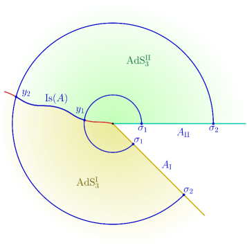
Figure 7: Schematics of the phase-II for the bulk geodesic homologous to the subsystem $A$ described by a finite interval $[\sigma_{1},\sigma_{2}]_{\text{I,II}}$ in dual CFT${}^{\text{I,II}}$. Here Is$(A)$ denotes the island region in the effective $2d$ description.

Doubly holographic description

For this phase, owing to the conventional island, the RT surface homologous to subsystem $A$ is composed of two single-crossing geodesics of the type discussed in section 4.1 and as depicted in fig. 7. Consequently, the candidate entanglement entropy for the present configuration may be expressed as

$$S_{\text{bulk}}=S_{\text{single}}(\sigma_{1},y_{1})+S_{\text{single}}(\sigma_{2},y_{2})\,.$$ (57)

As earlier, to obtain the locations of the common points $y_{i}$s on the EOW brane, we extremize the above with respect to $y_{1}$ and $y_{2}$ to obtain equations analogous to section 4 whose physical solutions will lead to the holographic entanglement entropy. Subsequently in the large tension limit described by eq. 45, this agrees with the corresponding result in the effective $2d$ description.

4.2.3 Phase - III

Effective $2d$ description

We now proceed to the final phase depicted in fig. 8 which involves the novel induced islands discussed in section 3.1. The location of this island region is described by $[a_{1},a_{2}]_{\text{I,II}}$ on the JT brane for the given subsystem. For this phase, we utilize the generalized entanglement entropy formula in eq. 40 for the corresponding subsystem $A$. The presence of induced island results in the factorization of the four-point twist correlators in the effective terms of the generalized entanglement entropy in the following way

$$\left<\mathcal{T}_{n}(\sigma_{1})\bar{\mathcal{T}}_{n}(\sigma_{2})\mathcal{T}_{n}(-a_{2})\bar{\mathcal{T}}_{n}(-a_{1})\right>_{\text{CFT}^{\text{I}}_{2}} =\left<\mathcal{T}_{n}(\sigma_{1})\bar{\mathcal{T}}_{n}(\sigma_{2})\right>_{\text{CFT}^{\text{I}}_{2}}\left<\mathcal{T}_{n}(-a_{1})\bar{\mathcal{T}}_{n}(-a_{2})\right>_{\text{CFT}^{\text{I}}_{2}}$$ (58)

$$\left<\mathcal{T}_{n}(\sigma_{1})\bar{\mathcal{T}}_{n}(\sigma_{2})\mathcal{T}_{n}(-a_{2})\bar{\mathcal{T}}_{n}(-a_{1})\right>_{\text{CFT}^{\text{II}}_{2}} =\left<\mathcal{T}_{n}(\sigma_{1})\bar{\mathcal{T}}_{n}(-a_{1})\right>_{\text{CFT}^{\text{II}}_{2}}\left<\mathcal{T}_{n}(\sigma_{2})\bar{\mathcal{T}}_{n}(-a_{2})\right>_{\text{CFT}^{\text{II}}_{2}}\,.$$

On utilization of the area term given in eq. 32 and the position dependent cut-off $\epsilon(y)$ on the JT brane, the generalized entanglement entropy in this case may then be expressed as

$$S_{\text{gen}}=\frac{\Phi_{r}}{a_{1}}+\frac{\Phi_{r}}{a_{2}}+\frac{c_{\text{I}}}{3}\log\left[\frac{1}{\cos\psi_{\text{I}}}\right]+\frac{c_{\text{II}}}{3}\log\left[\frac{1}{\cos\psi_{\text{II}}}\right]+\frac{c_{\text{I}}}{6}\log\left[\frac{\left(\sigma_{2}-\sigma_{1}\right)}{\epsilon}\right]$$ (59)

$$+\frac{c_{\text{I}}}{6}\log\left[\frac{\left(a_{1}-a_{2}\right)^{2}}{a_{1}\,a_{2}}\right]+\frac{c_{\text{II}}}{6}\log\left[\frac{\left(\sigma_{1}+a_{1}\right)^{2}}{\epsilon\,a_{1}}\right]+\frac{c_{\text{II}}}{6}\log\left[\frac{\left(\sigma_{2}+a_{2}\right)^{2}}{\epsilon\,a_{2}}\right]\,.$$

We now introduce a parameter $\Theta=\frac{\sigma_{2}}{\sigma_{1}}$ which is motivated from the analysis described in Anous:2022wqh . Moreover, one can also establish a similar relation between the QES $a_{1}$ and $a_{2}$ located on the JT brane as $a_{2}={\kappa}\,\Theta\,a_{1}$ where $\kappa$ is now one of the parameters whose extremal value will minimize the entanglement entropy. In the case of non-perturbed EOW brane where we obtain the usual ICFT₂ setup, it was shown in Anous:2022wqh that the current phase is only possible above a certain value of the parameter $\Theta$ depending upon the configuration of the EOW brane. Thus in our computations we assume $\Theta$ to be large. Finally, we introduce $\Theta$ and $\kappa$ in eq. 59, and extremize over the parameters $a_{1}$ and $\kappa$ in the large tension limit to obtain the following relations,

$$\partial_{\kappa}S_{\text{gen}}=0\quad\Rightarrow a_{1}\left(c_{\text{I}}+c_{\text{II}}\right)\kappa+\left(c_{\text{I}}-c_{\text{II}}\right)\sigma_{1}=0$$ (60)

$$\partial_{a_{1}}S_{\text{gen}}=0\quad\Rightarrow a_{1}\sigma_{1}\left(c_{\text{II}}\sigma_{1}+3(\kappa+1)\Phi_{r}\right)-a_{1}^{3}\kappa\,c_{\text{II}}+3a_{1}^{2}\kappa\,\Phi_{r}+3\sigma_{1}^{2}\Phi_{r}=0\,.$$

Solving the above, the extremal values of the QES are obtained to be

$$\kappa^{*}= \frac{\left(c_{\text{II}}-c_{\text{I}}\right)\,\sigma_{1}}{\left(c_{\text{I}}+c_{\text{II}}\right)\,a_{1}^{*}}\,$$ (61)

$$a_{1}^{*}= \frac{\left(c_{\text{I}}+c_{\text{II}}\right)\sigma_{1}+6\Phi_{r}+\sqrt{\left(\left(c_{\text{I}}+c_{\text{II}}\right)\sigma_{1}+6\Phi_{r}\right)^{2}+24\left(c_{\text{II}}-c_{\text{I}}\right)\sigma_{1}\Phi_{r}}}{2\left(c_{\text{II}}-c_{\text{I}}\right)}$$

where we have only considered the physical solutions of the island surfaces. The fine grained entropy for the subsystem $A$ may now be obtained by substituting the above extremal value in the generalized entropy in eq. 59.

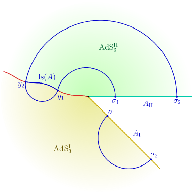
Figure 8: Schematics of the phase-III for the bulk geodesic homologous to the subsystem $A$ described by the finite interval $[\sigma_{1},\sigma_{2}]_{\text{I,II}}$ in dual CFT${}^{\text{I,II}}$. Here Is$(A)$ denotes the induced island region in the effective $2d$ description.

Doubly holographic description

In this subsection we obtain the length of the RT surfaces supported by the finite-sized subsystem $[\sigma_{1},\sigma_{2}]_{\rm I,II}$ located in the dual $\text{CFT}_{2}^{\rm I,II}$ as depicted in fig. 8. The interval in CFT${}_{2}^{\text{I}}$ supports the usual boundary anchored dome-shaped geodesic. However, for the interval in CFT${}_{2}^{\text{II}}$, the extremal curve is composed of three circular segments forming a double-crossing RT saddle as discussed in section 3.1. This double-crossing geodesic intersects the EOW brane at $y_{1}$ and $y_{2}$ which form the boundary of the island region in the effective $2d$ description.

Utilizing eq. 47, the length of the double-crossing geodesic may be obtained as

$$d= L_{\text{I}}\cosh^{-1}\left[\frac{\left(y_{2}-y_{1}\right){}^{2}\sin\psi_{\text{I}}(y_{1})\sin\psi_{\text{I}}(y_{2})+\left(y_{1}^{2}+y_{2}^{2}\right)\cos\psi_{\text{I}}(y_{1})\cos\psi_{\text{I}}(y_{2})}{2y_{1}y_{2}\cos\psi_{\text{I}}(y_{1})\cos\psi_{\text{I}}(y_{2})}\right]$$

$$+L_{\text{II}}\log\left[\frac{\left(\sigma_{1}+y_{1}\sin\psi_{\text{II}}(y_{1})\right){}^{2}+\left(y_{1}\cos\psi_{\text{II}}(y_{1})\right){}^{2}}{y_{2}\cos\psi_{\text{II}}(y_{1})}\right]$$

$$+L_{\text{II}}\log\left[\frac{\left(\sigma_{2}+y_{2}\sin\psi_{\text{II}}(y_{2})\right){}^{2}+\left(y_{2}\cos\psi_{\text{II}}(y_{2})\right){}^{2}}{y_{2}\cos\psi_{\text{II}}(y_{2})}\right]\,.$$ (62)

We may now introduce the variables $\Theta=\frac{\sigma_{2}}{\sigma_{1}}$ and $y_{2}=\hat{\kappa}\,\Theta\,y_{1}$, similar to the effective $2d$ perspective considered earlier. As advocated in Anous:2022wqh in the context of AdS₃/ICFT₂, such double-crossing geodesics are only permissible for large $\Theta$s. Consequently, in the large $\Theta$ limit of the above length, we obtain

$$d\approx L_{\text{I}}\log\left[\frac{\Theta\,\hat{\kappa}}{\cos\psi_{\rm I}(y_{1})\cos\psi_{\rm I}(y_{2})}\right] +L_{\text{II}}\log\left[\frac{\sigma_{1}^{2}+2y_{1}\sigma_{1}\sin\psi_{\rm II}(y_{1})+y_{1}^{2}}{y_{1}\cos\psi_{\rm II}(y_{1})}\right]$$ (63)

$$+L_{\text{II}}\log\left[\frac{\Theta(\sigma_{1}^{2}+2\hat{\kappa}y_{1}\sigma_{1}\sin\psi_{\rm II}(y_{2})+\hat{\kappa}^{2}y_{1}^{2})}{\hat{\kappa}\,y_{1}\cos\psi_{\rm II}(y_{2})}\right]\,.$$

Next we implement the position dependence of the brane angles $\psi_{\rm I,II}(y_{i})$ explicitly in the following way

$$\psi_{\rm I}(y_{i}) \to\sin^{-1}\left[\tanh\left(\frac{\rho^{0}_{\rm I}-\tilde{\rho}_{\rm I}\left(y_{i}\right)}{L_{\rm I}}\right)\right]\,,$$ (64)

$$\psi_{\rm II}(y_{i}) \to\sin^{-1}\left[\tanh\left(\frac{\rho^{0}_{\rm II}+\tilde{\rho}_{\rm II}\left(y_{i}\right)}{L_{\rm II}}\right)\right]~{}.$$

Expanding eq. 63 upto the leading order in $\tilde{\rho}_{\text{I,II}}$ and identifying the dilaton as in eq. 26, we may obtain the corresponding contribution from the double-crossing geodesic as follows

$$S_{\text{double}}(y_{1},y_{2})=\frac{\Phi_{r}}{y_{2}}+\frac{\Phi_{r}}{y_{1}}+\frac{L_{\text{I}}}{4G_{N}}\log\left[\frac{y_{2}}{y_{1}}\sec^{2}\left(\psi_{\rm I}\right)\right]$$

$$+\frac{L_{\text{II}}}{4G_{N}}\log\left[\frac{\left(\sigma_{2}^{2}+2y_{2}\,\sigma_{2}\sin\psi_{\rm II}+y_{2}^{2}\right)\left(\sigma_{1}^{2}+2y_{1}\,\sigma_{1}\sin\psi_{\rm II}+y_{1}^{2}\right)}{y_{1}\,y_{2}\cos^{2}\psi_{\rm II}}\right]~{},$$ (65)

where we have restored the original variables $\sigma_{2}$ and $y_{2}$.

Finally the candidate entanglement entropy for finite sized subsystem under consideration may be obtained by including the contribution from the dome-shaped geodesic as follows

$$S_{\text{bulk}} =S_{\text{double}}(y_{1},y_{2})+\frac{L_{\text{I}}}{4G_{N}}\log\left[\frac{\left(\sigma_{2}-\sigma_{1}\right)}{\epsilon\,\,}\right]\,.$$ (66)

The above may be extremized over the undetermined parameters $y_{1}$ and $y_{2}$ to obtain

$$2y_{1}\,\sigma_{1}\sin\psi_{\rm II}\left(4G_{N}\Phi_{r}\sin\psi_{\rm I}+L_{\rm I}y_{1}\right) +\sigma_{1}^{2}\left(4G_{N}\Phi_{r}\sin\left(\psi_{\rm I}\right)+\left(L_{\rm I}+L_{\rm II}\right)y_{1}\right)$$

$$\quad-y_{1}^{2}\left(\left(L_{\rm II}-L_{\rm I}\right)y_{1}-4G_{N}\Phi_{r}\sin\psi_{\rm I}\right)=0~{},$$ (67)

$$2y_{2}\,\sigma_{2}\sin\psi_{\rm II}\left(4G_{N}\Phi_{r}\sin\psi_{\rm I}-L_{\rm I}y_{2}\right) +\sigma_{2}^{2}\left(4G_{N}\Phi_{r}\sin\psi_{\rm I}-\left(L_{\rm I}-L_{\rm II}\right)y_{2}\right)$$

$$\quad-y_{2}^{2}\left(\left(L_{\rm I}+L_{\rm II}\right)y_{2}-4G_{N}\Phi_{r}\sin\psi_{\rm I}\right)=0~{}.$$ (68)

Solving the above equations for $y_{1}$ and $y_{2}$ and substituting the extremal values in eq. 66 will finally result in the holographic entanglement entropy for the given finite subsystem. Once again, in the large tension limit described in eq. 45, we observe that the corresponding entanglement entropy obtained through the effective $2d$ description is reproduced.

4.2.4 Page curve

We now plot the entanglement entropy for the finite subsystem $A$ under consideration in the dual CFT${}_{2}^{\text{I,II}}$s with respect to the subsystem size in fig. 9. For the given value of parameters, we observe transitions between the three phases discussed above as the subsystem size is increased. Initially when the subsystem is small in size, phase-I has the minimum entanglement entropy and is dominant. As we increase the subsystem size, subsequently phase-III starts dominating as crossing over to the region with smaller AdS radius AdS${}_{3}^{\text{I}}$, is more economical for the geodesic. Finally if the subsystem size is further increased, this advantage of double-crossing vanishes as the length of dome-shaped RT surface supported by the interval in CFT${}_{2}^{\text{I}}$ keeps increasing. And ultimately, phase-II becomes dominant.

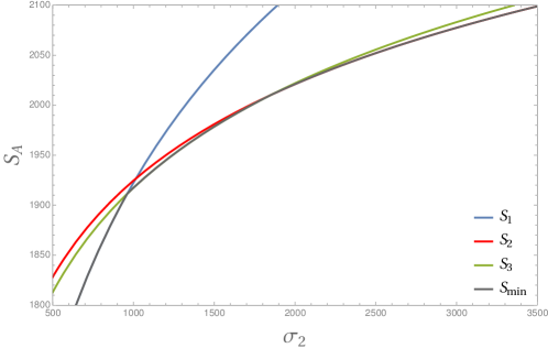
Figure 9: Variation of the entanglement entropy with the subsystem size ($\sigma_{2}$) for the finite sized subsystem $A$ where $c_{\text{I}}=35,c_{\text{II}}=800,\Phi_{r}=6.958,\delta=0.1,\sigma_{1}=0.4$. Here $S_{1},\,S_{2},\,S_{3}$ correspond to the entropy in phase-I, phase-II and phase-III respectively. The entanglement entropy is given by the minimum $S_{\text{min}}$ of these possible candidates for a given subsystem size.

5 Islands outside eternal JT black holes

In this section, we consider semi-infinite subsystems in thermal CFT₂ baths coupled to an eternal JT black hole. The thermofield double (TFD) state in this case may be constructed through the Euclidean path integral on half of an infinite cylinder Anous:2022wqh . The corresponding cylinder geometry may be obtained by applying a series of transformations on the planar ICFT₂ setup described by $\zeta=x+it_{E}$. We begin by mapping the flat interface to a circle of length $\ell$ through the following SL(2,$\mathbb{R}$) transformation

$$p=\frac{4\ell^{2}}{2\ell-\zeta}-\ell\,,$$ (69)

where $p=\tilde{x}+i\tilde{t}_{E}$. The corresponding bulk transformations may be obtained through the Bañados formalism Banados:1998gg ; Roberts:2012aq ; Shimaji:2018czt as follows

$$\tilde{x}=\frac{x-\frac{x^{2}+z^{2}-t^{2}}{2\ell}}{1-\frac{x}{\ell}+\frac{x^{2}+z^{2}-t^{2}}{4\ell^{2}}}+\ell\,,\qquad\tilde{z}=\frac{z}{1-\frac{x}{\ell}+\frac{x^{2}+z^{2}-t^{2}}{4\ell^{2}}}\,,\qquad\tilde{t}=\frac{t}{1-\frac{x}{\ell}+\frac{x^{2}+z^{2}-t^{2}}{4\ell^{2}}}\,.$$ (70)

We further obtain the cylinder geometry via the usual exponential map given by

$$p=\ell e^{\frac{2\pi}{\beta}q}~{},$$ (71)

where the coordinate $q=u+iv_{E}$ describes the cylinder with circumference $\beta$. The interface is now mapped to a circle $\mathfrak{R}\mathfrak{e}(q)=0$ with the two CFT₂s mapped on either side. The dual bulk theory for the TFD state on this cylinder is then described by an eternal black string spanning two AdS₃ geometries separated by a thin AdS₂ brane. The horizon of the black string crosses the brane and induces a horizon on it. A similar partial dimensional reduction as described in section 3 may now be performed for this $3d$ bulk to obtain an effective $2d$ description comprising of two thermal CFT₂ baths coupled to an eternal JT black hole.

In the cylinder coordinates, the metric and the dilaton profile for the eternal JT black hole in AdS₂ are given as follows Almheiri:2019hni ; Almheiri:2019qdq ; Almheiri:2019yqk

$$\textrm{d}s_{\text{grav}}^{2}=\frac{4\pi^{2}}{\beta^{2}}\frac{\text{d}q\,\text{d}\bar{q}}{\sinh^{2}\left(\frac{\pi(q+\bar{q})}{\beta}\right)}\quad, \Phi=\Phi_{0}-\frac{2\pi\Phi_{r}}{\beta}\coth\left(\frac{\pi(q+\bar{q})}{\beta}\right)\,,$$ (72)

where $\Phi_{0}$ is the topological contribution to the dilaton given in eq. 32. On the other hand, the metric for the CFT₂ baths may be expressed as

$$\textrm{d}s_{\text{bath}}^{2}=\frac{1}{\epsilon^{2}}\text{d}q\,\text{d}\bar{q}\,.$$ (73)

However, in the following we will employ the planar coordinates $p$ in which the field theory remains in the ground state and the corresponding stress tensor vanishes. The corresponding metrics and the dilaton are given as follows

$$\textrm{d}s_{\text{grav}}^{2}=\frac{4}{\left(1-|p|^{2}\right)^{2}}\text{d}p\,\text{d}\bar{p}\quad,\quad\textrm{d}s_{\text{bath}}^{2}=\frac{\beta^{2}}{4\pi^{2}\epsilon^{2}}\frac{\text{d}p\,\text{d}\bar{p}}{|p|^{2}}\,,$$

$$\qquad\qquad\qquad\Phi=\Phi_{0}+\frac{2\pi\Phi_{r}}{\beta}\frac{1+|p|^{2}}{1-|p|^{2}}\,.$$ (74)

We will now obtain the fine-grained entanglement entropy for a semi-infinite subsystem in bath CFT${}_{2}^{\text{I,II}}$s coupled to an eternal JT black hole. For this case, we observe two phases for the entanglement entropy as depicted in figs. 10 and 11. Specifically, for the first phase, we do not observe islands and obtain a steadily rising entanglement entropy as the black hole evolves. For the second phase, QES are observed outside the eternal JT black holes, indicating the presence of islands which saturates the entanglement entropy.

5.1 Phase - I

Effective $2d$ description

Now we describe the computation of the generalized entanglement entropy in the first phase for the subsystem composed of semi-infinite intervals $[P,\infty]_{\text{I}}\cup[R,\infty]_{\text{I}}$ considered in CFT${}_{2}^{\text{I}}$ bath and $[Q,\infty]_{\text{II}}\cup[S,\infty]_{\text{II}}$ in CFT${}_{2}^{\text{II}}$ bath as depicted in the fig. 10. Here the points $P$, $Q$ have coordinates as $(u_{0},v)_{\text{I,II}}$ in the cylinder coordinates and the points $R$, $S$ are their corresponding TFD copies with coordinates $(u_{0},-v+i\frac{\beta}{2})_{\text{I,II}}$. Note that in this case, the area term in the generalized entanglement entropy formula is vanishing as no island region is observed for this phase. The generalized entropy then involves only the effective term described by two two-point twist correlators and may be obtained to be

$$S_{A}=\frac{(c_{\text{I}}+c_{\text{II}})}{3}\log\left[\frac{\beta\cosh\left(\frac{2\pi v}{\beta}\right)}{\pi\,\epsilon}\right]\,.$$ (75)

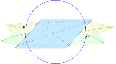
Figure 10: Schematics for the semi-infinite subsystem $A$ in phase-I where the extremal curve is composed of two Hartman-Maldacena surfaces.

Doubly holographic description

The double holographic description for this phase corresponds to the RT surfaces being composed of two Hartman-Maldacena (HM) surfaces stretched between the endpoints of the semi-infinite intervals on the asymptotic boundaries as depicted in fig. 10. The endpoints of the intervals are specified in the planer coordinates as $\tilde{x}_{1}(q_{1}^{\rm I})$ and $\tilde{x}_{1}(q_{1}^{\rm II})$ which may be obtained via the conformal maps eqs. 70 and 71. Consequently, in this phase the entanglement entropy corresponding to the HM surfaces may be obtained as

$$S_{\rm bulk} =\frac{L_{\text{I}}}{2G_{N}}\log\left[\frac{2\tilde{x}_{1}(q_{1}^{\rm I})}{\tilde{\epsilon}}\right]+\frac{L_{\text{II}}}{2G_{N}}\log\left[\frac{2\tilde{x}_{1}(q_{1}^{\rm II})}{\tilde{\epsilon}}\right]$$

$$=\frac{(L_{\text{I}}+L_{\text{II}})}{2G_{N}}\log\left[\frac{\beta\cosh\left(\frac{2\pi v}{\beta}\right)}{\pi\epsilon}\right]\,.$$ (76)

Note that the UV cut-offs between the two coordinates are related by $\tilde{\epsilon}(u,v)=\epsilon\,\frac{2\pi\ell}{\beta}e^{\frac{2\pi u}{\beta}}$. The above expression matches identically with the result obtained in the effective $2d$ description.

5.2 Phase - II

Effective $2d$ description

Now we describe the second phase for the generalized entropy of semi-infinite subsystems $[P,\infty]_{\text{I}}\cup[R,\infty]_{\text{I}}$ in CFT${}_{2}^{\text{I}}$ bath and $[Q,\infty]_{\text{II}}\cup[S,\infty]_{\text{II}}$ in CFT${}_{2}^{\text{II}}$ bath. Note that, as earlier, the points $P$, $Q$ are located at $(u_{0},v)_{\text{I,II}}$ in the cylinder coordinates and the points $R$, $S$ are their corresponding TFD copies. This phase involves a conventional island region bounded by the QES $M\equiv(-a,v_{a})_{\text{I,II}}$ and $N\equiv(-a,-v_{a}+i\frac{\beta}{2})_{\text{I,II}}$ on the JT brane leading to area terms in the generalized entanglement entropy. The effective terms in eq. 39 now involve four two-point twist correlators. The generalized entanglement entropy may then be obtained as

$$S_{\text{gen}}= \frac{4\pi\Phi_{r}}{\beta}\coth\left(\frac{2\pi a}{\beta}\right)+\frac{c_{\text{I}}}{3}\log\left[\frac{1}{\cos\psi_{\text{I}}}\right]+\frac{c_{\text{II}}}{3}\log\left[\frac{1}{\cos\psi_{\text{II}}}\right]$$ (77)

$$+\frac{(c_{\text{I}}+c_{\text{II}})}{3}\log\left[\frac{\left(e^{\frac{2\pi(-a-v_{a})}{\beta}}-e^{\frac{2\pi(u_{0}-v)}{\beta}}\right)\left(e^{\frac{2\pi(-a+v_{a})}{\beta}}-e^{\frac{2\pi(u_{0}+v)}{\beta}}\right)}{\frac{\pi\,\epsilon}{\beta}e^{\frac{2\pi u}{\beta}}\left(1-e^{\frac{-4\pi a}{\beta}}\right)}\right]\,.$$

We first extremize the above over the time $v_{a}$ of the QES to obtain the extremal value as

$$\partial_{v_{a}}S_{\text{gen}}=0 \Rightarrow\quad\quad v^{*}_{a}=v\,.$$ (78)

Subsequently, the extremization of the generalized entropy is performed over the location $a$ of the QES to obtain the following equation

$$\partial_{a}S_{\text{gen}}=0\quad\Rightarrow \frac{\sinh\left(\frac{\pi(a-u)}{\beta}\right)}{\sinh\left(\frac{\pi(a+u)}{\beta}\right)}=\frac{12\pi\Phi_{r}}{\beta\left(c_{\text{I}}+c_{\text{II}}\right)}\text{csch}\left(\frac{2\pi a}{\beta}\right)\,.$$ (79)

where we have implemented $v^{*}_{a}=v$. The fine grained entanglement entropy for this configuration may be obtained by solving the above for the extremal value $a^{*}$ and substituting it in eq. 77.

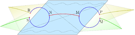
Figure 11: Schematics for the semi-infinite subsystem $A$ in phase-II where we observe the island region $NM$ on the JT brane in the effective $2d$ description.

Doubly holographic description

This subsection describes the doubly holographic computation of the entanglement entropy for the semi-infinite intervals in the dual CFT${}_{2}^{\text{I,II}}$s at a finite temperature as depicted in fig. 11. In particular, we compute the lengths of the RT surfaces homologous to the semi-infinite intervals. Similar to the previous case, we perform the computation in the planar coordinates where the endpoints of the intervals are described by $({x}_{0},{t}_{0})_{\text{I,II}}$ (and similarly for the TFD copies) in the dual CFT${}_{2}^{\text{I,II}}$s, whereas the island point on the EOW brane is located at ($y$, ${t}_{y}$). The length of the RT surface may now be obtained to be

$$d= {2L_{\text{I}}}\log\left[\frac{\left(x_{0}+y\sin\psi_{\text{I}}\right)^{2}+\left(t_{0}-t_{y}\right)^{2}+\left(y\cos\psi_{\text{I}}\right)^{2}}{\epsilon~{}y\cos\psi_{\text{I}}}\right]$$

$$+{2L_{\text{II}}}\log\left[\frac{\left(x_{0}+y\sin\psi_{\text{II}}\right)^{2}+\left(t_{0}-t_{y}\right)^{2}+\left(y\cos\psi_{\text{II}}\right)^{2}}{\epsilon~{}y\cos\psi_{\text{II}}}\right],$$ (80)

where the factor 2 arises from the symmetry of the TFD state. After introducing transverse fluctuations on the EOW brane and identifying the dilaton, the entanglement entropy may be expressed as

$$S_{\rm bulk}=\frac{2\Phi_{r}}{y} +\frac{L_{\text{I}}}{2G_{N}}\log\left(\frac{x_{0}^{2}+2x_{0}y\sin\psi_{\text{I}}+y^{2}}{\epsilon\,y\,\cos\psi_{\text{I}}}\right)$$

$$+\frac{L_{\text{II}}}{2G_{N}}\log\left(\frac{x_{0}^{2}+2x_{0}y\sin\psi_{\text{II}}+y^{2}}{\epsilon\,y\,\cos\psi_{\text{II}}}\right)\,,$$ (81)

where extremization over $t_{y}$ has been performed to set $t_{y}=t_{0}$. The location of the island $y$ may now be obtained by extremizing the above to obtain section 4 which may be transformed using the maps in eqs. 70 and 71 to obtain the corresponding extremization condition for the present scenario. Finally it may be observed that in the large tension limit the corresponding results match in the effective 2d theory.

5.3 Page curve

We now plot the Page curve for the entanglement entropy for the semi-infinite subsystem under consideration in the dual CFT${}_{2}^{\text{I,II}}$s at a finite temperature in fig. 12. We observe that, similar to the conventional scenarios with a single CFT₂ bath, initially phase-I is dominant with a monotonically increasing entanglement entropy and finally the island saddle for phase-II takes over when the entropy gets saturated to a constant value. This is expected as the presence of the additional bath does not affect the radiation process of the JT black hole. It just provides an additional reservoir for the Hawking radiations to be collected.

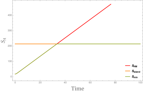
Figure 12: Page curve for semi-finite subsystem in the dual CFT${}^{\text{I,II}}$. Here we have chosen $c_{1}=6,c_{2}=12,u_{0}=10,\beta=2\pi,\epsilon=0.1$.

6 Islands and replica wormholes : gravity coupled with two baths

In this section, we investigate the replica wormhole saddle for the gravitational path integral and reproduce the location of the conical singularity and the entanglement entropy. We first perform the analysis for the effective lower dimensional model obtained from the AdS/ICFT setup by integrating out the bulk degrees of freedom, namely the “brane+bath” picture with topological gravity on the AdS₂ brane. Later on, we will include JT gravity on the brane and obtain the location of the island and the corresponding fine-grained entropy.

The procedure for obtaining the replica wormhole solutions from the boundary curve in two-dimensional gravity coupled to flat bath requires solving the so called conformal welding problem Almheiri:2019qdq ; Goto:2020wnk . The schematics of the welding problem is sketched in fig. 13. Essentially, the problem consists in finding a new Riemann surface out of two regions inside and outside of a disk which are described by different coordinate patches. Consider the regions parametrized by $|w|<1$ and $|v|>1$ which are glued together along their boundaries at $|v|=|w|=1$, where the complex coordinates are described by

$$v=e^{y}=e^{\sigma+i\tau}~{}~{},~{}~{}w=e^{\gamma+i\theta}\,.$$ (82)

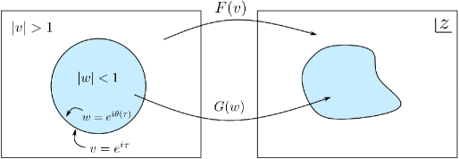
Figure 13: The conventional conformal welding problem Almheiri:2019qdq . The two disks $|v|>1$ and $|w|<1$ are glued in terms of the boundary mode $\theta(\tau)$, where $w=e^{i\theta(\tau)}$ and $v=e^{i\tau}$.

It is, in general, impossible to extend the coordinates $w$ or $v$ holomorphically beyond the respective boundary circles. However, by virtue of the Riemann mapping theorem, one can find two holomorphic functions $F$ and $G$ to establish another coordinate system $z$ on a new Riemann surface such that the regions $|w|<1$ and $|v|>1$ are holomorphically mapped to the coordinate $z$. In other words, one requires

$$z=G(w)~{}~{},~{}~{} \text{for}~{}|w|<1$$

$$z=F(v)~{}~{},~{}~{} \text{for}~{}|v|>1$$ (83)

$$G\left(e^{i\theta(\tau)}\right)=F\left(e^{i\tau}\right)~{}~{},~{}~{} \text{for}~{}|v|=|w|=1\,.$$

The problem of finding holomorphic $F(v)$ and $G(w)$ given the boundary mode $\theta(\tau)$ is termed the conformal welding problem. In the case of two dimensional gravity on a AdS₂ manifold coupled to a flat CFT₂ bath such a welding issue arises naturally Almheiri:2019qdq ; Goto:2020wnk . In the presence of dynamical gravity, the entanglement entropy for a subsystem is computed through the Lewkowycz-Maldacena procedure by considering an $n$-fold cover of the original manifold $\mathcal{M}$ Lewkowycz:2013nqa . For a replica symmetric saddle $\mathcal{M}_{n}$ to the gravitational path integral, it is convenient to quotient by the $\mathbb{Z}_{n}$ replica symmetry and consider a single manifold $\tilde{\mathcal{M}}_{n}=\mathcal{M}_{n}/\mathbb{Z}_{n}$. The orbifold $\tilde{\mathcal{M}}_{n}$ essentially describes a disk with conical singularities at which twist operators for the conformal matter theory are inserted. The metric on the interior manifold $\tilde{\mathcal{M}}_{n}$ may be described by a complex coordinate $w$ as follows:

$$\text{d}s^{2}=e^{2\rho(w,\bar{w})}\text{d}w\text{d}\bar{w}~{}~{},~{}~{}\text{for}|w|<1\,.$$ (84)

In a finite temperature configuration with $\tau\sim\tau+2\pi$, in order to join the metric of the quotient manifold of the gravitating region to the flat space outside described by the exterior coordinates $v=e^{y}$, it is required to solve the conformal welding problem discussed above. In this case, the boundary mode $\theta(\tau)$ plays the role of the reparametrization mode in two-dimensional gravity Almheiri:2019qdq .

6.1 Replica wormholes from AdS/ICFT

In this subsection, we focus on the replica wormhole solutions in the framework of AdS/ICFT discussed in Anous:2022wqh and briefly reviewed in section 2. In the effective lower dimensional scenario obtained from integrating out the bulk spacetimes on either side of the brane $\sigma$, we have two flat baths attached to the gravitational region on the EOW brane $\Sigma$ which has a weakly gravitating metric in the large tension limit. There are two CFTs along the flat half lines which extends to the gravitating region where they interact via the weakly fluctuating metric. The schematics of the setup is sketched in fig. 14.

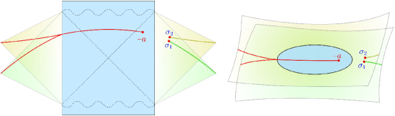
Figure 14: The single sided configuration in the Lorentzian signature (left) and in the Euclidean signature (right).

As discussed earlier, for a quantum field theory coupled to dynamical gravity on a hybrid manifold, the replica trick to compute the entanglement entropy for a subsystem involves a replication of the original manifold in the replica index $n$. The normalized partition function $\mathbf{Z}_{n}$ on this replica manifold then computes the entanglement entropy as follows Lewkowycz:2013nqa ; Almheiri:2019qdq

$$S=-\partial_{n}\left(\frac{\log\mathbf{Z}_{n}}{n}\right)\Bigg{|}_{n=1}\,.$$ (85)

The partition function for the gravity region concerns a gravitational path integral which may be solved in the saddle-point approximation in the semi-classical regime by specifying appropriate boundary conditions. These saddles may be characterized by the nature of gluing of the individual replica copies. In particular, two specific choices will be of importance for our purposes, namely the Hawking saddle where the $n$-copies of the bath(s) are glued cyclically while gravity is filled in each copy individually, and the replica wormhole saddle in which along with the copies of the bath, gravitational regions are dynamically glued together. In these replica wormhole saddles, upon quotienting via the replica symmetry $\mathbb{Z}_{n}$, additional conical singularities dynamically appear at the fixed points of the replica symmetry in the orbifold theory.

The gravitational action on the orbifold $\tilde{\Sigma}_{n}$ obtained by quotienting the replicated EOW brane $\Sigma_{n}$ is given by

$$-\frac{1}{n}I_{\text{grav}}\big{[}\tilde{\Sigma}_{n}\big{]}=\sum_{k=\text{I},\text{II}}\frac{L_{k}}{32\pi G_{N}}\int_{\Sigma}\text{d}^{2}y\sqrt{-\tilde{h}}\,\bigg{[}R^{(2)}-R^{(2)} \log\left(-\frac{L^{2}_{k}}{2}R^{(2)}\right)\bigg{]}$$

$$- \left(1-\frac{1}{n}\right)\sum_{i}S(w_{i})\,,$$ (86)

where $S(w_{i})$ denotes the contributions from the dynamical conical singularities. In our case, this is just a constant given in eq. 30 with a vanishing dilaton term.

We choose the complex coordinate $w$ to describe the gravity region inside the disk $|w|=1$. Furthermore, the baths outside the disk are described by the complex coordinates $v_{k}\,,(k=\text{{I,II}})$, in the spirit of eq. 82. Then the conformal welding problem sketched in fig. 15 is reduced to the determination of the appropriate boundary mode $\theta(\tau)$. We consider two semi-infinite intervals in the bath CFT${}_{2}^{\text{I,II}}$s as $[\sigma_{1},\infty]_{\text{I}}$ and $[\sigma_{2},\infty]_{\text{II}}$ and in the replica manifold twist operators are placed at the locations $v_{\text{I}}=e^{\sigma_{1}}$ and $v_{\text{II}}=e^{\sigma_{2}}$. Note that for the replica wormhole saddle, a dynamical conical singularity also appears at $w=e^{-a}$.

To proceed, we now require the energy flux equation at the interface of the gravitational region and the bath CFTs. The variation of the gravitational action with respect to the boundary mode is vanishing

$$-\frac{1}{n}\,\delta I_{\text{grav}}=0\,.$$ (87)

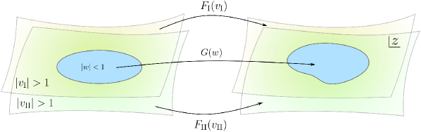
Figure 15: Conformal welding problem for our setup with two CFT₂ baths defined in the regions $|v_{\text{I}}|>1$ and $|v_{\text{II}}|>1$ which are coupled to gravity inside the circle $|w|<1$.

On the other hand, the variation of the matter partition function $\mathbf{Z}_{\text{mat}}$ with respect to the boundary mode leads to the following expression Almheiri:2019qdq

$$\delta\log\mathbf{Z}_{\text{mat}}=i\int\text{d}\tau\sum_{k=\text{I},\text{II}}\left(T^{(k)}_{yy}-T^{(k)}_{\bar{y}\bar{y}}\right)\frac{\delta\theta(\tau)}{\theta^{\prime}(\tau)}$$ (88)

Utilizing the above equations, the energy flux condition at the boundary may be expressed as follows

$$i\left[T^{(\text{I})}_{yy}(i\tau)-T^{(\text{I})}_{\bar{y}\bar{y}}(-i\tau)\right]+i\left[T^{(\text{II})}_{yy}(i\tau)-T^{(\text{II})}_{\bar{y}\bar{y}}(-i\tau)\right]=0\,.$$ (89)

Under the conformal map $y\to z=F_{k}(v_{k})$, the energy momentum tensor transforms as

$$T^{(k)}_{yy}(i\tau)\to e^{2y}\left[\left(\frac{dF_{k}(e^{y})}{dv_{k}}\right)^{2}T^{(k)}_{zz}-\frac{c_{k}}{24\pi}\left\{F_{k}(e^{y}),v_{k}\right\}\right]~{}~{},~{}~{}k=\text{I},\text{II}$$ (90)

In the replicated geometry, the uniformization map for the conical singularities is given by $z\to\tilde{z}=z^{1/n}$ such that $T^{({k})}_{\tilde{z}\tilde{z}}=0$ and the energy-momentum tensors for the two CFTs in the $z$-plane is given by

$$T^{({k})}_{zz}=-\frac{c_{k}}{24\pi}\left(1-\frac{1}{n^{2}}\right)\frac{1}{z^{2}}\,.$$ (91)

Therefore, the energy-flux condition in eq. 89 reduces to

$$0=\sum_{k=\text{I},\text{II}}ie^{2i\tau}c_{k}\left[\frac{1}{2}\left(1-\frac{1}{n^{2}}\right)\left(\frac{{F_{k}}^{\prime}(e^{i\tau})}{F_{k}(e^{i\tau})}\right)^{2}+\left\{F_{k}(e^{i\tau}),e^{i\tau}\right\}\right]+\text{c.c.}\,.$$ (92)

Since the maps $F_{k}$ depend on the gluing function $\theta(\tau)$, the above equation is in general hard to solve. However, one may solve it near $n=1$ as described below.

For $n=1$, the first term in the parenthesis of eq. 92 vanishes and the welding is trivial. Therefore, we may conclude that the maps $F_{k}$ are well approximated near $n=1$ by Möbius transformations of the form

$$z=F_{k}(v_{k})=\frac{v_{k}-\mathcal{A}}{\mathcal{B}_{k}-v_{k}}~{}~{},~{}~{}\mathcal{A}=e^{-a}~{},~{}\mathcal{B}_{\text{I}}=e^{\sigma_{1}}~{},~{}\mathcal{B}_{\text{II}}=e^{\sigma_{2}}$$ (93)

It is straightforward to verify that these functions indeed map the branch points at $-a$ and $\sigma_{1,2}$ to $z=0$ and $z=\infty$ respectively. Therefore, the energy flux condition becomes

$$c_{\text{I}}\mathcal{F}_{\text{I}}+c_{\text{II}}\mathcal{F}_{\text{II}}=0\,,$$ (94)

where

$$\mathcal{F}_{k}=ie^{2i\tau}\left(\frac{{F_{k}}^{\prime}\left(e^{i\tau}\right)}{F_{k}\left(e^{i\tau}\right)}\right)^{2}+\text{c.c.}=ie^{2i\tau}\frac{(\mathcal{A}-\mathcal{B}_{k})^{2}}{\left(e^{-i\tau}-\mathcal{A}\right)^{2}\left(e^{i\tau}-\mathcal{B}_{k}\right)^{2}}+\text{c.c.}$$ (95)

Now, performing a Fourier transformation in the above equation (restoring the temperature $\beta$), the expression for the $k=1$ mode reads

$$0 =\int_{0}^{\beta}\,\text{d}\tau\,e^{-\frac{2\pi i\tau}{\beta}}\left(c_{\text{I}}\mathcal{F}_{\text{I}}+c_{\text{II}}\mathcal{F}_{\text{II}}\right)$$

$$=c_{\text{I}}\left(\frac{\sinh\left[\frac{\pi(a-\sigma_{1})}{\beta}\right]}{\sinh\left[\frac{\pi(a+\sigma_{1})}{\beta}\right]}\right)+c_{\text{II}}\left(\frac{\sinh\left[\frac{\pi(a-\sigma_{2})}{\beta}\right]}{\sinh\left[\frac{\pi(a+\sigma_{2})}{\beta}\right]}\right)$$ (96)

In order to compare with the quantum extremal surface condition at zero temperature, we now take the $\beta\to\infty$ limit to obtain

$$0=c_{\text{I}}\left(\frac{a-\sigma_{1}}{a+\sigma_{1}}\right)+c_{\text{II}}\left(\frac{a-\sigma_{2}}{a+\sigma_{2}}\right)\,,$$ (97)

which on solving for $a$ gives

$$a^{*}=\frac{(c_{\text{I}}-c_{\text{II}})\left(\sigma_{1}-\sigma_{2}\right)+\sqrt{4\left(c_{\text{I}}+c_{\text{II}}\right)^{2}\sigma_{1}\sigma_{2}+\left(c_{\text{I}}-c_{\text{II}}\right)^{2}\left(\sigma_{1}-\sigma_{2}\right)^{2}}}{2\left(c_{\text{I}}+c_{\text{II}}\right)}\,.$$ (98)

The above expression is identical to the position of the quantum extremal surface obtained through extremizing the generalized entropy in Anous:2022wqh .

6.2 Replica wormholes with JT gravity coupled to two baths

With JT gravity on the EOW brane $\Sigma$, the energy flux condition at the boundary of the replicated geometry is modified and the conformal welding problem is a bit more involved. The variation of the gravitational action with respect to the boundary mode $\theta(\tau)$ no longer vanishes since in the case of JT gravity $\theta(\tau)$ serves as the “boundary graviton” Almheiri:2019qdq . The energy flux condition in the presence of JT gravity on the brane is then modified to Almheiri:2019qdq ; Goto:2020wnk ; Suzuki:2022xwv

$$\partial_{\tau}M=i\left[T^{(\text{I})}_{yy}(i\tau)-T^{(\text{I})}_{\bar{y}\bar{y}}(-i\tau)\right]+i\left[T^{(\text{II})}_{yy}(i\tau)-T^{(\text{II})}_{\bar{y}\bar{y}}(-i\tau)\right]$$ (99)

where $M$ corresponds to the ADM mass of the gravitational theory which is related to the Schwarzian boundary action.

For the two single intervals $[\sigma_{1},\infty]_{\text{I}}$ and $[\sigma_{2},\infty]_{\text{II}}$ on CFT${}_{2}^{\text{I,II}}$ baths, a conical singularity appears inside the gravity region on the orbifold theory $\Sigma_{n}/\mathbb{Z}_{n}$ at a point $-a$ and we need to consider the subsystems $[-\infty,-a]_{\text{I}}\cup[\sigma_{1},\infty]_{\text{I}}$ and $[-\infty,-a]_{\text{II}}\cup[\sigma_{2},\infty]_{\text{II}}$. Once again, we will work with a finite temperature configuration with $\beta=2\pi$. We may now uniformize the interior conical singularity at $w=\mathcal{A}=e^{-a}$ by utilizing the map

$$\tilde{w}=\left(\frac{w-\mathcal{A}}{1-\mathcal{A}\,w}\right)^{\frac{1}{n}}\,.$$ (100)

In the $\tilde{w}$ coordinates, the gravity region has the usual hyperbolic disk metric Almheiri:2019qdq

$$\text{d}s^{2}_{\text{in}}=\frac{4\text{d}\tilde{w}\text{d}\bar{\tilde{w}}}{\left(1-|\tilde{w}|^{2}\right)^{2}}\,.$$ (101)

In these coordinates we may set $\tilde{w}=e^{i\tilde{\theta}}$ at the boundary. Now using the Schwarzian composition rules, we may obtain the ADM mass of the spacetime to be Almheiri:2019qdq

$$\frac{\Phi_{r}}{4\pi}\left\{e^{i\tilde{\theta}},\tau\right\}=\frac{\Phi_{r}}{4\pi}\left[\left\{e^{i\theta},\tau\right\}+\frac{1}{2}\left(1-\frac{1}{n^{2}}\right)R(\theta)\right]\,,$$ (102)

where the function $R(\theta)$ contains the information about the branch point $-a$ as follows

$$R(\theta)=-\frac{(1-\mathcal{A}^{2})^{2}(\partial_{\tau}\theta)^{2}}{|1-\mathcal{A}\,e^{i\theta}|^{4}}\,.$$ (103)

Now, utilizing eqs. 92, 99 and 102, the energy flux condition at the boundary becomes

$$-\frac{12\Phi_{r}}{c} \partial_{\tau}\left[\left\{e^{i\theta},\tau\right\}+\frac{1}{2}\left(1-\frac{1}{n^{2}}\right)R(\theta)\right]$$

$$=\sum_{k=\text{I},\text{II}}ie^{2i\tau}c_{k}\left[\frac{1}{2}\left(1-\frac{1}{n^{2}}\right)\left(\frac{{F_{k}}^{\prime}(e^{i\tau})}{F_{k}(e^{i\tau})}\right)^{2}+\left\{F_{k}(e^{i\tau}),e^{i\tau}\right\}\right]+\text{c.c.}$$ (104)

The above relation is quite complicated as the map $F$ depends implicitly on the gluing function $\theta(\tau)$. Nevertheless, as earlier, we may solve it near $n\sim 1$ as follows. Near $n\sim 1$, we may expand the boundary mode $\theta(\tau)$ as follows Almheiri:2019qdq

$$e^{i\theta(\tau)}=e^{i\tau}\left[1+i\delta\theta(\tau)\right]\,,$$ (105)

where $\delta\theta(\tau)$ is of order $(n-1)$. Next we use the following relation Almheiri:2019qdq

$$e^{2i\tau}\left\{F_{k},e^{i\tau}\right\}=-\frac{1}{2}(1+H)(\delta\theta^{\prime\prime\prime}+\delta\theta^{\prime})\,,$$ (106)

where $H$ is the Hilbert transform which projects out the negative frequency modes of $\delta\theta$. Note that, except for in the Schwarzian term $\left\{F_{k},e^{i\tau}\right\}$, the functions $F_{k}$ appear with a factor of $(n-1)$ in eq. 104 and we may keep only up to the zeroth order solutions given in eq. 93. Restoring the temperature dependence utilizing the scaling $\Phi_{r}\to\frac{2\pi\Phi_{r}}{\beta}$ and Fourier transforming to the $k$ basis, the $k=1$ mode requires

$$\int_{0}^{\beta}\text{d}\tau\,e^{-\frac{2\pi i\tau}{\beta}}\left[c_{\text{I}}\mathcal{F}_{\text{I}}+c_{\text{II}}\mathcal{F}_{\text{II}}-\frac{{24\pi\Phi_{r}}}{\beta}\partial_{\tau}R(\tau)\right]=0$$ (108)

which leads to the condition

$$c_{\text{I}}\left(\frac{\sinh\left[\frac{\pi(a-\sigma_{1})}{\beta}\right]}{\sinh\left[\frac{\pi(a+\sigma_{1})}{\beta}\right]}\right)+c_{\text{II}}\left(\frac{\sinh\left[\frac{\pi(a-\sigma_{2})}{\beta}\right]}{\sinh\left[\frac{\pi(a+\sigma_{2})}{\beta}\right]}\right)=\frac{{12\pi\Phi_{r}}}{\beta}\text{csch}\left(\frac{2\pi a}{\beta}\right)$$ (109)

In the $\beta\to\infty$ limit, this reduces to a cubic equation in $a$ as follows

$$c_{\text{I}}\left(\frac{a-\sigma_{1}}{a+\sigma_{1}}\right)+c_{\text{II}}\left(\frac{a-\sigma_{2}}{a+\sigma_{2}}\right)=\frac{6\Phi_{r}}{a}$$ (110)

The above equation is easily solved for $a$ but the solutions are not quite illuminating. Instead, we take the simplifying limit $\sigma_{1}=\sigma_{2}=\sigma$ to get the quadratic equation

$$a(a-\sigma)-\frac{6\Phi_{r}}{\left(c_{\text{I}}+c_{\text{II}}\right)}(a+\sigma)=0\,.$$ (111)

Solving for the position of the conical singularity $a$, we obtain

$$a^{*}=\frac{\left(c_{\text{I}}+c_{\text{II}}\right)\sigma+6\Phi_{r}+\sqrt{\left(\left(c_{\text{I}}+c_{\text{II}}\right)\sigma+6\Phi_{r}\right)^{2}+24\left(c_{\text{I}}+c_{\text{II}}\right)\sigma\Phi_{r}}}{2\left(c_{\text{I}}+c_{\text{II}}\right)}$$ (112)

which is identical to the position of the QES obtained in section 4.1.

7 Summary and discussion

In this article, we have investigated the entanglement structure of various bipartite states in a hybrid manifold where a JT gravity is coupled to two non-gravitating CFT₂ baths. To this end, we first construct this hybrid theory through a dimensional reduction of a $3d$ geometry. The $3d$ geometry is comprised of a fluctuating EOW brane acting as an interface between two distinct AdS₃ geometries. Performing a partial Randall-Sundrum reduction in the neighbourhood of the fluctuating brane results in JT gravity on the EOW brane. Furthermore, utilizing the usual AdS/CFT correspondence on the remaining wedges of the two AdS₃ geometries leads to two non-gravitating CFT baths on two half lines. In the limit of large brane tension, we obtain the $2d$ effective theory of JT gravity coupled to conformal matter on the hybrid “brane+baths” manifolds.

Furthermore, we have provided a prescription for computing the generalized Rényi entropy for a subsystem in this hybrid manifold. In particular, for this scenario where the JT gravity is coupled to two CFT₂ baths, the dominant replica wormhole saddle is modified to provide two independent mechanisms to obtain an island region. Other than the conventional origin of the island region where the degrees of freedom for the CFT in the gravitational region is shared by bath CFTs, we also observe cases where island region is captured for CFT${}^{\text{I}}$ even though no bath degrees of freedom is considered. We have called such regions as the induced islands, as the subsystem purely in CFT${}^{\text{II}}$ induces an island region even for CFT${}^{\text{I}}$. In the doubly holographic perspective this phenomena corresponds to the double-crossing geodesic where the RT surface crosses from AdS${}^{\text{II}}$ to AdS${}^{\text{I}}$ and returns to AdS${}^{\text{II}}$.

Subsequently, we obtain the entanglement entropy for subsystems comprised of semi-infinite and finite intervals in CFT${}_{2}^{\text{I,II}}$ coupled to extremal as well as eternal JT black holes. We perform computations from the effective $2d$ perspective using the generalized entanglement entropy formula and find agreement with the doubly holographic computation in the large tension limit of the EOW brane for all the cases. We also plot Page curves for the different configurations of the subsystems and observe transitions between different phases of the entanglement entropy.

We have also performed the so called conformal welding problem for the replica wormhole saddle in the effective “brane+bath” scenario and obtained the location of the island for semi-infinite subsystems in the baths. To this end, we begin with the lower dimensional effective picture obtained from the AdS/ICFT setup discussed in Anous:2022wqh and reproduce the QES result. Subsequently, this is extended to the case with JT gravity on the EOW brane which substantiate the island computations for the corresponding configuration.

There are several future directions to explore. For finite intervals in the baths coupled to JT gravity, the location of the islands may be obtained through the conformal welding problem with the replica wormhole by extending of the analysis in Goto:2020wnk . It will be interesting to explore the nature of mixed state entanglement in Hawking radiation from the JT black hole via different entanglement and correlation measures such as the reflected entropy Dutta:2019gen , the entanglement negativity Calabrese:2012nk , the entanglement of purification Takayanagi:2017knl and the balanced partial entanglement Wen:2021qgx . Furthermore, our setup can be extended to include holographic models of interface CFTs which involve two interface branes separating three bulk regions Baig:2022cnb . A partial dimensional reduction on different bulk wedges would result in two fluctuating JT branes with black holes which interact through the CFT₂ baths on a hybrid seagull-like geometry. This provides yet another exotic model of Hawking radiation which may lead to new insights for the information loss problem.

- (1) G. Penington, Entanglement Wedge Reconstruction and the Information Paradox, JHEP 09 (2020) 002 [1905.08255].
- (2) G. Penington, S. H. Shenker, D. Stanford and Z. Yang, Replica wormholes and the black hole interior, JHEP 03 (2022) 205 [1911.11977].
- (3) A. Almheiri, R. Mahajan, J. Maldacena and Y. Zhao, The Page curve of Hawking radiation from semiclassical geometry, JHEP 03 (2020) 149 [1908.10996].
- (4) A. Almheiri, T. Hartman, J. Maldacena, E. Shaghoulian and A. Tajdini, Replica Wormholes and the Entropy of Hawking Radiation, JHEP 05 (2020) 013 [1911.12333].
- (5) A. Almheiri, R. Mahajan and J. Maldacena, Islands outside the horizon, 1910.11077.
- (6) D. N. Page, Information in black hole radiation, Phys. Rev. Lett. 71 (1993) 3743 [hep-th/9306083].
- (7) D. N. Page, Average entropy of a subsystem, Phys. Rev. Lett. 71 (1993) 1291 [gr-qc/9305007].
- (8) D. N. Page, Time Dependence of Hawking Radiation Entropy, JCAP 09 (2013) 028 [1301.4995].
- (9) J. Sully, M. V. Raamsdonk and D. Wakeham, BCFT entanglement entropy at large central charge and the black hole interior, JHEP 03 (2021) 167 [2004.13088].
- (10) M. Rozali, J. Sully, M. Van Raamsdonk, C. Waddell and D. Wakeham, Information radiation in BCFT models of black holes, JHEP 05 (2020) 004 [1910.12836].
- (11) H. Z. Chen, R. C. Myers, D. Neuenfeld, I. A. Reyes and J. Sandor, Quantum Extremal Islands Made Easy, Part I: Entanglement on the Brane, JHEP 10 (2020) 166 [2006.04851].
- (12) H. Z. Chen, R. C. Myers, D. Neuenfeld, I. A. Reyes and J. Sandor, Quantum Extremal Islands Made Easy, Part II: Black Holes on the Brane, JHEP 12 (2020) 025 [2010.00018].
- (13) G. Grimaldi, J. Hernandez and R. C. Myers, Quantum extremal islands made easy. Part IV. Massive black holes on the brane, JHEP 03 (2022) 136 [2202.00679].
- (14) K. Suzuki and T. Takayanagi, BCFT and Islands in two dimensions, JHEP 06 (2022) 095 [2202.08462].
- (15) F. Deng, J. Chu and Y. Zhou, Defect extremal surface as the holographic counterpart of Island formula, JHEP 03 (2021) 008 [2012.07612].
- (16) J. Chu, F. Deng and Y. Zhou, Page curve from defect extremal surface and island in higher dimensions, JHEP 10 (2021) 149 [2105.09106].
- (17) T. Takayanagi, Holographic Dual of BCFT, Phys. Rev. Lett. 107 (2011) 101602 [1105.5165].
- (18) M. Fujita, T. Takayanagi and E. Tonni, Aspects of AdS/BCFT, JHEP 11 (2011) 043 [1108.5152].
- (19) J. Kastikainen and S. Shashi, Structure of holographic BCFT correlators from geodesics, Phys. Rev. D 105 (2022) 046007 [2109.00079].
- (20) T. Li, M.-K. Yuan and Y. Zhou, Defect extremal surface for reflected entropy, JHEP 01 (2022) 018 [2108.08544].
- (21) D. Basu, H. Parihar, V. Raj and G. Sengupta, Defect extremal surfaces for entanglement negativity, 2205.07905.
- (22) Y. Shao, M.-K. Yuan and Y. Zhou, Entanglement Negativity and Defect Extremal Surface, 2206.05951.
- (23) Y. Lu and J. Lin, The Markov gap in the presence of islands, JHEP 03 (2023) 043 [2211.06886].
- (24) R. Jackiw, Lower Dimensional Gravity, Nucl. Phys. B 252 (1985) 343.
- (25) C. Teitelboim, Gravitation and Hamiltonian Structure in Two Space-Time Dimensions, Phys. Lett. B 126 (1983) 41.
- (26) F. Deng, Y.-S. An and Y. Zhou, JT gravity from partial reduction and defect extremal surface, JHEP 02 (2023) 219 [2206.09609].
- (27) H. Geng, A. Karch, C. Perez-Pardavila, S. Raju, L. Randall, M. Riojas et al., Jackiw-Teitelboim Gravity from the Karch-Randall Braneworld, Phys. Rev. Lett. 129 (2022) 231601 [2206.04695].
- (28) H. Geng, Aspects of AdS2 quantum gravity and the Karch-Randall braneworld, JHEP 09 (2022) 024 [2206.11277].
- (29) E. Verheijden and E. Verlinde, From the BTZ black hole to JT gravity: geometrizing the island, JHEP 11 (2021) 092 [2102.00922].
- (30) J. Kumar Basak, D. Basu, V. Malvimat, H. Parihar and G. Sengupta, Page curve for entanglement negativity through geometric evaporation, SciPost Phys. 12 (2022) 004 [2106.12593].
- (31) T. Anous, M. Meineri, P. Pelliconi and J. Sonner, Sailing past the End of the World and discovering the Island, SciPost Phys. 13 (2022) 075 [2202.11718].
- (32) E. Sharon and D. Mumford, 2D-Shape Analysis Using Conformal Mapping, Int J Comput Vision 70 (2006) 55.
- (33) K. Goto, T. Hartman and A. Tajdini, Replica wormholes for an evaporating 2D black hole, JHEP 04 (2021) 289 [2011.09043].
- (34) S. Fallows and S. F. Ross, Islands and mixed states in closed universes, JHEP 07 (2021) 022 [2103.14364].
- (35) K. Skenderis and S. N. Solodukhin, Quantum effective action from the AdS / CFT correspondence, Phys. Lett. B 472 (2000) 316 [hep-th/9910023].
- (36) X. Dong, X.-L. Qi, Z. Shangnan and Z. Yang, Effective entropy of quantum fields coupled with gravity, JHEP 10 (2020) 052 [2007.02987].
- (37) S. Ryu and T. Takayanagi, Holographic derivation of entanglement entropy from AdS/CFT, Phys. Rev. Lett. 96 (2006) 181602 [hep-th/0603001].
- (38) J. D. Brown and M. Henneaux, Central Charges in the Canonical Realization of Asymptotic Symmetries: An Example from Three-Dimensional Gravity, Commun. Math. Phys. 104 (1986) 207.
- (39) M. Banados, Three-dimensional quantum geometry and black holes, AIP Conf. Proc. 484 (1999) 147 [hep-th/9901148].
- (40) M. M. Roberts, Time evolution of entanglement entropy from a pulse, JHEP 12 (2012) 027 [1204.1982].
- (41) T. Shimaji, T. Takayanagi and Z. Wei, Holographic Quantum Circuits from Splitting/Joining Local Quenches, JHEP 03 (2019) 165 [1812.01176].
- (42) A. Lewkowycz and J. Maldacena, Generalized gravitational entropy, JHEP 08 (2013) 090 [1304.4926].
- (43) S. Dutta and T. Faulkner, A canonical purification for the entanglement wedge cross-section, JHEP 03 (2021) 178 [1905.00577].
- (44) P. Calabrese, J. Cardy and E. Tonni, Entanglement negativity in extended systems: A field theoretical approach, J. Stat. Mech. 1302 (2013) P02008 [1210.5359].
- (45) T. Takayanagi and K. Umemoto, Entanglement of purification through holographic duality, Nature Phys. 14 (2018) 573 [1708.09393].
- (46) Q. Wen, Balanced Partial Entanglement and the Entanglement Wedge Cross Section, JHEP 04 (2021) 301 [2103.00415].
- (47) S. A. Baig and A. Karch, Double brane holographic model dual to 2d ICFTs, JHEP 10 (2022) 022 [2206.01752].