Localised Dynamics in the Floquet Quantum East Model

Abstract

We introduce and study the discrete-time version of the Quantum East model, an interacting quantum spin chain inspired by simple kinetically constrained models of classical glasses. Previous work has established that its continuous-time counterpart displays a disorder-free localisation transition signalled by the appearance of an exponentially large (in the volume) family of non-thermal, localised eigenstates. Here we combine analytical and numerical approaches to show that: i) The transition persists for discrete times, in fact, it is present for any finite value of the time step apart from a zero measure set; ii) It is directly detected by following the non-equilibrium dynamics of the fully polarised state. Our findings imply that the transition is currently observable in state-of-the-art platforms for digital quantum simulation.

Introduction.— Establishing the precise conditions for real space localisation in interacting systems, even in one dimension, turns out to be extremely challenging. In fact, despite intense efforts to crack it [1, 2, 3, 4, 5, 6, 7, 8, 9], it currently remains a major unsolved problem in theoretical physics. It has been argued that a form of many-body localisation should emerge as a consequence of an external quenched disorder, which, under some conditions, might defeat interactions. Whether this mechanism can lead to a stable phase of matter, however, is still a matter of an active debate [7, 8, 9]. A fundamental problem in all these studies is that they are either limited to small systems accessible to numerical or experimental simulation or uncontrolled perturbative approximations. Nevertheless, if many-body localisation can ever be established as a phase of matter it has to exist in the thermodynamic limit, meaning it should not (only) be the property of eigenstates, but (also) of time evolution (dynamics) of an infinite system.

Recently, it has been suggested that, other than by disorder, real space localisation can also be triggered by kinetic constraints which render transport a higher-order process. An advantage of this approach is that it is not affected by fluctuating rare events such as ergodic bubbles. A minimal example of this mechanism is realised in the so-called Quantum East model [10, 11, 12, 13, 14] (and its bosonic version [15]) where a localisation transition in the quantum Hamiltonian is in one-to-one correspondence to a first order activity-inactivity transition in the corresponding classical stochastic glass model. Consistently with this picture, Ref. [16] observed an eigenstate localisation transition in the Quantum East for an exponentially large family of eigenstates.

In this work, we take a fundamental step further and look for the possibility of dynamical localisation in a Floquet, or trotterised, version of the Quantum East model. We replace the continuous Hamiltonian dynamics by a discrete sequence of conditional unitary gate operations – a quantum circuit – that can be conveniently implemented on platforms for digital quantum simulation such as trapped ions [17, 18, 19, 20] and superconducting circuits [21, 22, 23, 24, 25, 26]. Using time-dependent perturbation theory, we argue that the model displays a localisation transition by tuning the parameters of the model. We demonstrate that in the dynamically localised phase the model can be efficiently simulated by time-dependent matrix product methods (i.e. TEBD algorithm) [27, 28, 29] to an arbitrary precision, showing very good quantitative agreement with the perturbative prediction. Moreover, we find qualitative agreement between dynamical picture of localisation in the infinite system and localisation of eigenstates in the finite system.

The model.— Our starting point is the Quantum East model [10], which is defined by the following Hamiltonian operator (in arbitrary energy units)

$$H(a)=\sum_{j=1}^{2L-1}P_{j}(aX_{j+1}-I)+aX_{1}-I\,.$$ (1)

Here $a$ is the dimensionless coupling constant, $2L$ is the system size, $\{X_{j},Y_{j},Z_{j}\}$ are Pauli matrices acting non-trivially at site $j$, $I$ is the identity operator, and $P_{j}=(I+Z_{j})/2$.

We are interested in discrete sequences of unitary operations $\mathbb{U}(a,\tau)$ that reproduce the dynamics generated by Eq. (1) in a special scaling limit. Namely

$$\lim_{t\to\infty}\mathbb{U}(a,\mathfrak{t}/t)^{t}=e^{-iH(a)\mathfrak{t}}\,.$$ (2)

This procedure is known as Trotter-Suzuki decomposition [30, 31] and does not uniquely specify the unitary operator: there are many different choices of $\mathbb{U}(a,\tau)$ fulfilling Eq. (2). Here we consider a simple one that is local in space, i.e., it has the following brickwork structure (see Fig. 1)

$$\mathbb{U}(a,\tau)=e^{i\tau}\mathbb{U}_{\rm e}(a,\tau)\mathbb{U}_{\rm o}(a,\tau),$$ (3)

with

$$\mathbb{U}_{\rm e}(a,\tau)=U_{1,2}(a,\tau)\cdots U_{2L-1,2L}(a,\tau),$$

$$\mathbb{U}_{\rm o}(a,\tau)=e^{-i\tau aX_{1}}U_{2,3}(a,\tau)\cdots U_{2L-2,2L-1}(a,\tau),$$ (4)

where we use a standard notation $O_{x,y}$ for an operator $O$ acting non-trivially only at the sites $x$ and $y$, and define a local conditional gate

$$U(a,\tau)=e^{-i\tau(aP\otimes X-P\otimes I)}\,.$$ (5)

The time step $\tau$, usually referred to as the Trotter step, sets the strength of the unitary operation (3). It is easy to verify that (2) holds for the evolution operator defined in Eq. (3).

Figure 1: (Left) State (6) after $t=3.5$ time steps of discrete dynamics. White bullets denote the state $\ket{\downarrow}$ and the blue circles the activation part of the conditional gate $U(a,\tau)$. In yellow we highlighted the brick-wall Floquet propagator $\mathbb{U}(a,\tau)$. (Right) Explicit simplification of the dynamics out of the light cone. With dashed line we indicated the cut for the ladder evolution in Eq. (8). In orange we highlighted the ladder propagator $\mathbb{U}_{\ell}(a,\tau)$ (cf. (9)).

To probe the localisation properties of the quantum circuit (3) we consider a local quantum quench. Namely, we prepare the circuit in the initial state

$$\ket{\downarrow\cdots\downarrow},$$ (6)

which is an eigenstate of the bulk evolution due to the identity ${U(a,\tau)\ket{\downarrow\downarrow}=\ket{\downarrow\downarrow}},$ but is not stationary at the left boundary. A direct consequence of this is that only the sites within a light cone spreading from the left boundary undergo a non-trivial evolution. Specifically, at time $t$ only the $2t$ leftmost sites are affected by the time evolution, see Fig. 1. Intuitively, one can think of our local quench protocol as creating a localised disturbance in $(x,t)=(0,0)$ in a state that is otherwise stationary.

A simple measure of how the disturbance created by the local quench spreads through the system is given by the partial norms

$$W(x,t)\!=\!\!\!\sum_{s_{j}=\uparrow,\downarrow}|\!\matrixelement{s_{1}\ldots s_{x-1}\!\!\uparrow\downarrow\!\cdots\!\!\downarrow}{\mathbb{U}(a,\tau)^{t}}{\downarrow\!\cdots\!\downarrow}\!|^{2}\!.$$ (7)

Since ${W(x,t)\geq 0}$ and ${\sum_{x}W(x,t)=1}$, the partial norms can be thought of as the probability of having the rightmost up spin at position $x$. Specifically, whenever the disturbance remains localised at the boundary we have $W(x,t)\approx 0$ for $x\gg x_{0}=O(t^{0})$, while when it spreads through the light cone the partial norms attain non-zero values for all $x\leq 2t$. Note that, because of the light cone structure of the dynamics, one always has ${W(x>2t,t)=0}$.

In fact, to facilitate our numerical analysis here we consider slightly modified quantities that bear the same physical information as those in Eq. (7): Instead of the partial norms of the state $\mathbb{U}(a,\tau)^{t}\ket{\downarrow\!\cdots\!\downarrow}$, we look at those of the state along the diagonal cut in the right panel of Fig. 1. The latter quantities are defined as

$$N(x,t)\!=\!\!\!\!\!\sum_{s_{j}=\uparrow,\downarrow}\!\!|\!\matrixelement{s_{1}\ldots s_{x-1}\!\!\uparrow\downarrow\!\cdots\!\!\downarrow}{\mathbb{U}_{\ell}(a,\tau)^{t}}{\downarrow\!\cdots\!\downarrow}\!|^{2}\!\!,$$ (8)

where we introduced the “ladder evolution operator” (cf. Fig 1)

$$\,\,\!\!\!\!\mathbb{U}_{\ell}(a,\!\tau\!)\!=\!e^{i\tau}\!e^{-i\tau aX_{1}}U_{1,2}(a,\!\tau\!)U_{2,3}(a,\!\tau\!)\!\cdots\!U_{L-1,L}(a,\!\tau\!),$$ (9)

which is related to $\mathbb{U}(a,\tau)$ by a similarity transformation [32]. The quantities in Eq. (8) are more convenient than those in Eq. (7) because with the same computational effort one can access times that are twice as long.

Infinite system at finite times.— Let us begin considering the time evolution of the partial norms $N(x,t)$ in the thermodynamic limit $L\to\infty$. In this case, the main qualitative features of their evolution can be understood by performing a simple perturbative analysis (the same can be done for $W(x,t)$ [32]). We begin by introducing the interaction representation of the time evolution operator

$${\mathbb{U}}_{\ell}(a,\tau)^{t}=\left[\prod_{k=0}^{t}\tilde{\mathbb{U}}_{\ell}(\tau a,\tau k)\right]e^{i\tau t\sum_{j}\!P_{j}},$$ (10)

where we defined

$$\tilde{\mathbb{U}}_{\ell}(a,\tau)=e^{i\tau}e^{-iaX_{1}e^{-i\tau Z_{1}}}\!\!\!\prod_{k\in\{1,\ldots 2L-1\}}^{\rightarrow}\!\!\!\tilde{U}_{k,k+1}(a,\tau),$$ (11)

$$\tilde{U}(a,\tau)=e^{-iaP\otimes Xe^{-i\tau Z}}\,.$$ (12)

We now fix $x,t,\tau$ and expand (7) in powers of $a$. Looking at the local gate in the interaction picture, i.e.,

$$\tilde{U}_{1,2}(a,\tau)=\mathbbm{1}-iaP_{1}X_{2}e^{-i\tau Z_{2}}+O(a^{2})\,$$ (13)

we have that $N(x)$ is at least of order $a^{2x}$. Indeed, due to the structure of Eq. (3), to get a spin up at position $x$ we need to at least flip all the spins on its left. In fact, this also tells us

$$\!\!\!\!\!N(x,t)\!\simeq\!N^{\prime}(x,t)\!\equiv\!|\!\matrixelement*{\underbrace{\uparrow\cdots\uparrow}_{x}\downarrow\!\cdots\!\downarrow}{\mathbb{U}(a,\tau)^{t}}{\downarrow\!\cdots\!\downarrow}\!|^{2}\!\!,$$ (14)

where $\simeq$ denotes equality at the leading order in $a$. Evaluating the corresponding amplitude

$$A^{\prime}(x,t)=\matrixelement*{\underbrace{\uparrow\cdots\uparrow}_{x}\downarrow\cdots\downarrow}{\mathbb{U}_{\ell}(a,\tau)^{t}}{\downarrow\cdots\downarrow},$$ (15)

at leading order is a simple combinatorial problem: we plug (13) and (10) into (15) and count the number ways to flip $x$ spins in sequential order. For the $j$-th flip we get a factor $ia\tau e^{i\tau t_{j}}$, where ${t\leq t_{j}<t_{j-1}}$ is the time of the $j$-th flip. This gives

$$A^{\prime}(x,t)\simeq(-i)^{x}e^{i\tau t}(a\tau)^{x}K(x,t),$$ (16)

where we introduced

$$K(x,t)\equiv\sum_{t_{1}=1}^{t}\sum_{t_{2}=t_{1}+1}^{t}\cdots\!\!\!\!\!\sum_{t_{x}=t_{x-1}+1}^{t}e^{i\tau(t_{1}+\cdots+t_{x})}.$$ (17)

It is simple to show that these objects fulfil the following recurrence relations

$$K(x,t)=K(x,t-1)+K(x-1,t-1)e^{i\tau t},$$ (18)

with $K(x>t,t)=0$ and $K(0,0)=1$ which is solved by

$$K(x,t)=e^{-i\tau x(x+1)/2}\begin{pmatrix}t\\ x\end{pmatrix}_{\!\!\!q}\!\!.$$ (19)

Here we set $q\equiv e^{i\tau}$ and

$$\!\!\!\!\!\begin{pmatrix}n\\ m\end{pmatrix}_{\!\!\!q}\!\!=\!\frac{[n]_{q}!}{[n-m]_{q}![m]_{q}!},\,\,n\geq m,\quad\begin{pmatrix}n\\ m\end{pmatrix}_{\!\!\!q}\!\!=0,\,\,n<m,$$ (20)

are $q$-deformed binomial coefficients defined in terms of $q$-deformed factorials

$$[n]_{q}!=\prod_{k=1}^{n}[n]_{q},\qquad[k]_{q}=\frac{1-q^{k}}{1-q}\,.$$ (21)

Putting all together we then find

$$N(x,t)\simeq N^{\prime}_{1}(x,t)\equiv(a\tau)^{2x}\biggl{|}\!\begin{pmatrix}t\\ x\end{pmatrix}_{\!\!\!q}\biggr{|}^{2}\!\!,$$ (22)

which concludes the perturbative calculation. Interestingly, this perturbative analysis commutes with the limit (2). Indeed

$$\lim_{\tau\to 0}N^{\prime}_{1}(x,\mathfrak{t}/\tau)=\frac{(2a\sin(\mathfrak{t}/2))^{2x}}{(x!)^{2}},$$ (23)

coincides with the leading order of (8) if one replaces (10) with its Trotter limit [32].

Let us now move on to analyse the localisation properties of the perturbative solution. To this aim, we assume that $N^{\prime}_{1}(x,t)$ gives the only relevant contribution to the partial norm. The first key feature of $N^{\prime}_{1}(x,t)$ is that its localisation properties depend on whether or not $\tau$ is a rational multiple of $2\pi$. Namely, whether it can be written as ${2\pi c}/{d}$ for some coprime integers $c$ and $d$. When this is the case one can use the $q$-Lucas theorem [33] to connect the behaviour of $q$-deformed and regular binomials as follows

$$\begin{pmatrix}t\\ x\end{pmatrix}_{\!\!\!q}=\begin{pmatrix}\lfloor t/d\rfloor\\ \lfloor x/d\rfloor\end{pmatrix}\begin{pmatrix}{\rm mod}(t,d)\\ {\rm mod}(x,d)\end{pmatrix}_{\!\!\!q}\,,$$ (24)

where $\lfloor x\rfloor$ is the largest integer smaller than $x$ and ${\rm mod}(c,d)$ is the remainder of the division of $c\in\mathbb{N}$ by $d\in\mathbb{N}$. Using now the Stirling approximation we find that Eq. (22) has a maximum at

$$\bar{x}=\frac{(a\tau)^{2d}t}{1+(a\tau)^{2d}}\,.$$ (25)

Therefore the support of $N^{\prime}_{1}(x,t)$ grows in time ruling out localisation.

On the other hand, whenever $\tau$ is not a rational multiple of $2\pi$ the deformed binomial coefficients are bounded in time. Namely we have

$$\log\left|\begin{pmatrix}t\\ x\end{pmatrix}_{\!\!\!q}\right|^{2}= \sum_{p=1}^{t-x}\log\left[\frac{1-\cos(\tau(x+p))}{1-\cos(\tau p)}\right]\simeq O(t^{0}).$$ (26)

In the last step we used that, since $\{{\rm mod}(\tau p,2\pi)\}_{p=1}^{t}$ covers $[0,2\pi)$ uniformly in the large $t$ limit, we have

$$\sum_{p=1}^{t-x}\log(1-\cos(\tau(y+p)))\simeq(x-t)\log 2\,,\quad\forall y\,.$$ (27)

Therefore the $O(t)$ in Eq. (26) cancels and we are left with an $O(t^{0})$ term. Plugging the bound Eq. (26) into Eq. (22) we have that $N^{\prime}_{1}(x,t)$ is localised within a distance $x_{0}={-1}/{(2\log a\tau)}$ from the left boundary for all times.

The second key feature that we can extract from the perturbative solution is the $\tau$ dependence of $a_{c}$ — the critical $a$ for localisation — in the case of irrational $\tau/(2\pi)$. In our setup this amounts to ask for what range of $a$ we expect the perturbative result to apply (at least qualitatively). From Eq. (22) we see that for finite $\tau$ the parameter that has to be small to ensure the validity of the perturbative approach is $a\tau$. Instead, in the limit $\tau\to 0$ the perturbative solution requires $a$ itself to be small [32]. This suggests that $a_{c}$ should be of the form

$$a_{c}(\tau)=\min(\alpha,\beta/\tau)\,,$$ (28)

for some $\alpha,\beta\in\mathbb{R}$.

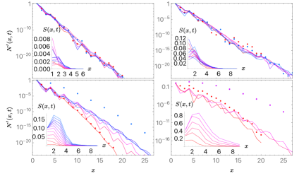
Figure 2: Profiles of $N^{\prime}(x,t)$ for $a=0.1$ (left column panels), $a=0.2$ (right column panels), and for $\tau=(\sqrt{5}-1)\pi/2$ (top row panels), $\tau=2\pi/3$ (bottom row panels). The data are shown for times $t=20,40\ldots 120$ (red to blue curves), except for bottom/right panel where only $t=20,40,60$ can be computed due to fast growth of entanglement (insets indicate entanglement entropy profiles $S(x,t)$, $t=10,20\ldots$, of respective cases). Coloured bullets depict perturbative results for shortest and longest simulated time.

Remarkably, by computing $N(x,t)$ and $N^{\prime}(x,t)$ via a simple version of the TEBD algorithm [32] we find that all these qualitative features persist away from the perturbative regime. Some representative examples of our numerical results are presented in Figs. 2 and 3, where, as a further indicator of localisation, we also report the entanglement entropy $S(x,t)$ between the $x$ leftmost sites and the rest of the system at time $t$.

For small enough $a$ we see that disturbance created by the local quench remains localised only for irrational values of $\tau/(2\pi)$. This is clearly shown in the insets of Fig. 2: While for rational $\tau/(2\pi)$ we see the peak of the entanglement entropy growing linearly in time, for irrational $\tau/(2\pi)$ we see it saturating. Moreover, while in the former case the peak’s distance from the left edge also grows linearly in time, in the latter it approaches a time-independent value. Note that we observe this stark difference between rational and irrational $\tau/(2\pi)$ also for times that are significantly out of the perturbative regime ($t\gg 1/a$) and at which Eq. (22) is not quantitatively accurate: see the comparison in the main panel of Fig. 2. As a result of this localised behaviour, for irrational $\tau/(2\pi)$ we are able to run our TEBD simulations with essentially no truncation error for hundreds of time steps.

On the other hand, for $a$ larger than a certain critical value $a_{c}(\tau)$ the system transitions to the ergodic regime also for irrational $\tau/(2\pi)$, see Fig. 3. In this case the perturbative result does not describe the system’s behaviour even at the qualitative level: the support of the partial norms grows linearly in time signalling a delocalisation of the disturbance caused by the impurity. Concerning the $\tau$ dependence of $a_{c}(\tau)$, our numerical results are compatible with the functional form in Eq. (28) [32]. Namely, the critical $a$ appears approximately $\tau$-independent for small $\tau$ , while it starts to decay as $\tau^{-1}$ when $\tau$ is increased beyond a threshold value.

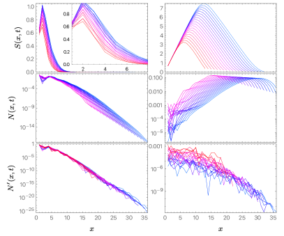
Figure 3: Two cases of ergodic finite $t$/infinite size dynamics: left, right, column panels correspond, respectively, to $a=0.3,\tau=(\sqrt{5}-1)\pi/2$ just beyond localization transition, and to $a=1.0,\tau=(\sqrt{5}-1)\pi/2$ well in the ergodic phase. We plot entanglement entropy profiles $S(x,t)$, partial norm profiles $N(x,t)$, and domain wall component profiles $N^{\prime}(x,t)$, in lines 1 to 3 respectively, for $t=17,18\ldots 36$ (red to blue).

Finite systems at infinite times.—

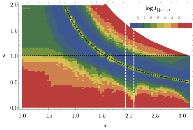
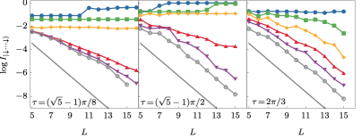
Figure 4: (Top) Logarithm of the IPR at $L=13$ as a function of $\tau$ and $a$. We see that for small $\tau$ the transition is at $a=1$, whereas for bigger $\tau$ the transition is at $a\propto 1/\tau$. With the white dashed lines we show the three values of $\tau$ considered in the bottom panel. (Bottom) Logarithm of the IPR versus $L$ for three values of $\tau$ and several values of $a$ ($0.5,0.7,\dots,1.5$ top to bottom for the first plot and $0.05,0.15,\dots,0.55$ for the second and third). The grey solid line corresponds to fastest decay $2^{-L}$ for random eigenstates. For the first two values of $\tau$, we can estimate the transition between constant and exponential decay at $a=1$ and $a=0.3$. The third $\tau$ is a rational multiple of $2\pi$, and its transition occurs at a much smaller $a$.

Interestingly, the phenomenology observed above in the thermodynamic limit setting is also observed for finite volumes. In this case we again look at a quench from the initial state in Eq. (6) but keep $L$ finite while taking ${t\to\infty}$. A convenient indicator of the localisation transition is then the time averaged square of Loschmidt Echo (LE) $|\bra{\downarrow\cdots\downarrow}\mathbb{U}_{\ell}^{t}\ket{\downarrow\cdots\downarrow}|^{2}$ [this quantity is the same for brick-wall $\mathbb{U}$ and ladder propagators $\mathbb{U}_{\ell}$]. Assuming that there are no degeneracies in the spectrum of $\mathbb{U}_{\ell}$, the LE can be written as

$$\lim_{t\to\infty}\frac{1}{t}\sum_{s}^{t}|\bra{\downarrow\cdots\downarrow}{\mathbb{U}_{\ell}(a,\tau)}^{s}\ket{\downarrow\cdots\downarrow}|^{2}$$

$$=\!\!\lim_{t\to\infty}\!\frac{1}{t}\!\sum_{s}^{t}\sum_{i,j}|\!\bra{\downarrow\cdots\downarrow}\ket{E_{i}}\!|^{2}|\!\bra{\downarrow\cdots\downarrow}\ket{E_{j}}\!|^{2}e^{i(E_{j}-E_{i})s}$$

$$=\sum_{i}|\bra{\downarrow\cdots\downarrow}\ket{E_{i}}|^{4}\equiv I_{\ket{\downarrow\cdots\downarrow}},$$ (29)

where the sum over $i,j$ goes over all of the eigenstates. The quantity on the last line is the so called inverse participation ratio (IPR), which measures the spreading of the initial state in the eigenbasis of the time-evolution operator. It can be interpreted as the purity of the probability distribution $\{P_{i}\}$, with $P_{i}=|\bra{\downarrow\cdots\downarrow}\ket{E_{i}}|^{2}$ being the Born probability of measuring the eigenstate $\ket{E_{i}}$ in $\ket{\downarrow\cdots\downarrow}$.

For random eigenstates $\ket{E_{i}}$ the probability distribution is flat, i.e., $P_{i}={2^{-L}}$, which gives $I_{\ket{\downarrow\cdots\downarrow},\text{Haar}}={2^{-L}}$. In contrast, in the localised phase, we expect that up to exponential corrections, the initial state spreads up to a finite distance $k$, so $\mathbb{U}^{t}\ket{\downarrow\cdots\downarrow}=\ket{\psi}\ket{\downarrow}^{\otimes(L-k)}$, which leads to an IPR constant in $L$. Namely $I_{\ket{\downarrow\cdots\downarrow},\text{loc}}\geq{2^{-k}}$ for all $L$.

We computed $I_{\ket{\downarrow\cdots\downarrow}}$ numerically for several values of $a$, $\tau$, and $L$: our main numerical results are summarised in Fig. 4. We see that IPR versus $a$ and $\tau$ produces a suggestive phase diagram, where the localisation transitions matches the finite time data surprisingly well. The bottom panel of the figure shows the IPR versus $L$ for different values $a$ and three choices of $\tau$. Identifying the localisation transition as the transition between constant and exponentially decaying IPR, we can estimate $a_{c}(\tau)$. The last two $\tau$ are similar in size, but they are respectively irrational and rational multiples of $2\pi$. We see that the difference between these two cases is stark also in this setting: the irrational $\tau/(2\pi)$ shows a transition at sizeable $a$, while $\tau/(2\pi)$ shows ergodic behaviour for the same choice of $a$. In the phase diagram, the rational $\tau/(2\pi)$ generate some irregular behaviour reminiscent of Arnold tongues [34]. Some further finite-volume data is reported in the SM [32].

Conclusions and Outlook.— We introduced a discrete-time version of the Quantum East model [10] and analysed its localisation properties in real-time. Specifically, we studied the spreading of disturbances that are initially spatially localised. Combining a perturbative analysis with exact numerics we identified a localisation transition taking place in this system as a function of the dimensionless coupling $a$: for couplings smaller than a critical value $a_{c}(\tau)$ the effect of the disturbance remains localised in space, while it spreads ballistically for $a>a_{c}(\tau)$. This is also shown by a stark difference in the entanglement scaling (linear vs bounded). Interestingly, this transition has a non-analytic dependence on the Trotter time $\tau$ and takes place only when the latter is an irrational multiple of $2\pi$.

Our work opens several directions for future research. First, it calls for a more precise and systematic characterisation of the observed transition. Since the entanglement appears to be exactly bounded in the localised phase, many features of this transition can be efficiently characterised via tensor network methods. Moreover, the discrete space-time setting introduced in this letter is particularly convenient for analytical analyses. Second, more generally, our work shows that quantum circuits composed of one-sided control gates, like our Floquet Quantum East, can generate interesting minimal models where one can exactly study exotic physical behaviours.

Supplementary Material for:
“Localised Dynamics in the Floquet Quantum East Model”

Appendix A Perturbative analysis of $W(x,t)$

The perturbative analysis of the main text can be directly performed also for the partial norms $W(x,t)$ in the brickwall formulation, Eq. (7). Considering the interaction picture representation of the evolution operator (3) we have

$$\!\!\!\!{\mathbb{U}(a,\tau)^{t}}e^{i\tau t(1+\sum_{j}\!P_{j})}\!\!=\!\!\prod_{k=0}^{t-1}\!\tilde{\mathbb{U}}_{\rm e}(\tau a,k\tau)\tilde{\mathbb{U}}_{\rm o}(\tau a,(k+1)\tau),$$ (SA.1)

where we introduced

$$\tilde{\mathbb{U}}_{\rm e}(a,\tau)=\tilde{U}(a,\tau)^{\otimes L},$$ (SA.2)

$$\tilde{\mathbb{U}}_{\rm o}(a,\tau)=e^{-iaX}\otimes\tilde{U}(a,\tau)^{\otimes(L-1)}\,,$$ (SA.3)

and $\tilde{U}(a,\tau)$ is the one given in Eq. (12). Considering the amplitude

$$A^{\prime}_{W}(x,t)=\matrixelement*{\underbrace{\uparrow\cdots\uparrow}_{x}\downarrow\cdots\downarrow}{\mathbb{U}(a,\tau)^{t}}{\downarrow\cdots\downarrow}$$ (SA.4)

we find that it is again computed by counting the number ways to flip $x$ spins in sequential order. This time the $j$-th flip gives a factor

$$-ia\tau e^{-i\tau(t-t_{j}+{\rm mod}(j,2))},$$ (SA.5)

where $t\leq t_{j}\leq t_{j-1}+{\rm mod}(j,2)$. Putting all together we find

$$A^{\prime}_{W}(x,t)\simeq(-i)^{x}e^{-i\tau[t(x+1)+\lceil x/2\rceil]}(a\tau)^{x}C(x,t),$$ (SA.6)

where we introduced

$$C(x,t)=\sum_{p_{1}=1}^{t}\sum_{p_{2}=p_{1}}^{t}\cdots\!\!\!\!\!\sum_{p_{x}=p_{x\!-\!1}+{\rm mod}(x,2)}^{t}\!\!\!\!\!\!e^{i\tau(p_{1}+\cdots+p_{x})}.$$ (SA.7)

The coefficients $C(x,t)$ fulfil the following recursive relation

$$C(2x,t)=\,C(2x,t\!-\!1)+C(2x\!-\!1,t\!-\!1)e^{i\tau t}+C(2x-2,t\!-\!1)e^{2i\tau t},$$ (SA.8)

$$C(2x\!-\!1,t)=C(2x\!-\!1,t\!-\!1)+C(2x\!-\!2,t\!-\!1)e^{i\tau t}\!\!\!,$$ (SA.9)

with boundary conditions

$$\!\!\!C(0,1)=1,\quad C(1,1)=e^{i\tau},\quad C(2,1)=e^{2i\tau}\!\!,$$ (SA.10)

$$\!\!\!C(x<0,t)=0,\quad C(x>2t,t)=0.$$ (SA.11)

These equations are solved by

$$\!\!C(x,t)=q^{x/2+x^{2}/4+{\rm mod}(x,2)/4}\begin{pmatrix}t+\lfloor x/2\rfloor\\ x\end{pmatrix}_{q=e^{i\tau}}\!\!\!.$$ (SA.12)

Plugging back into (14) we finally find

$$W(x,t)\simeq(a\tau)^{2x}\left|C(x,t)\right|^{2}\,.$$ (SA.13)

Appendix B Perturbation theory in the Trotter limit

Considering the Trotter limit of the time-evolution operator in the interaction picture we have

$$\lim_{\tau\to 0}{\mathbb{U}}(a,\tau)^{\mathfrak{t}/\tau}={\rm T}\!\exp\left[-i\int_{0}^{\mathfrak{t}}{\rm d}sH_{I}(s,a)\right]e^{i\mathfrak{t}\sum_{j}\!P_{j}},$$ (SB.14)

where ${\rm T}\!\exp[\cdot]$ represents the time-ordered exponential and

$$H_{I}(s,a)=a\sum_{j}P_{j}X_{j+1}e^{-isZ_{j+1}}+a(X_{1}e^{-isZ_{1}}-\mathbbm{1}),$$ (SB.15)

is the coupling part of the Hamiltonian in the interaction representation. A standard expansion of the time-ordered exponential gives

$$A^{\prime}(x,t)= \matrixelement*{\underbrace{\uparrow\cdots\uparrow}_{x}\downarrow\cdots\downarrow}{{\rm T}\!\exp\left[-i\int_{0}^{\mathfrak{t}}{\rm d}sH_{I}(s,a)\right]}{\downarrow\cdots\downarrow}$$

$$= (-i)^{x}a^{x}\matrixelement*{\underbrace{\uparrow\cdots\uparrow}_{x}\downarrow\cdots\downarrow}{X_{x}P_{x-1}\ldots X_{2}P_{1}X_{1}}{\downarrow\cdots\downarrow}\int_{0}^{\mathfrak{t}}{\rm d}t_{x}\int_{0}^{t_{x}}{\rm d}t_{x-1}\cdots\int_{0}^{t_{2}}{\rm d}t_{1}e^{i(t_{x}+\ldots+t_{1})}+O(a^{x+1})$$

$$= (-2ia)^{x}\frac{\sin(\mathfrak{t}/2)^{x}}{x!}\,.$$ (SB.16)

Plugging back into Eq. (14) we find Eq. (23).

Appendix C TEBD algorithm for conditional ladder circuit

To simulate the dynamics in the Floquet Quantum East circuit in the ladder formulation we use the standard time-evolved block decimation (TEBD) algorithm [27], which is ideally suited for this particular application. We write the state

$$\ket{\psi(t)}=\mathbb{U}_{\ell}^{t}\ket{\downarrow\downarrow\cdots}$$ (SC.17)

which we represent as a matrix product state

$$\ket{\psi(t)}=\sum_{s_{1},\ldots,s_{t}\in\{\uparrow,\downarrow\}}A^{(1,t)}_{s_{1}}\Lambda^{(1,t)}A^{(2,t)}_{s_{2}}\Lambda^{(2,t)}\cdots A^{(t,t)}_{s_{t}}\ket{s_{1}s_{2}\cdots s_{t}\downarrow\downarrow\cdots}.$$ (SC.18)

$A^{(x,t)}$ are $d^{(x-1,t)}\times d^{(x,t)}$ dimensional matrices, which at any position $x\in\{1,\ldots,t\}$ and instant of time $t\in\mathbb{N}$ satisfy the (right) orthogonality relations

$$\sum_{s\in\{\uparrow,\downarrow\}}A^{(x,t)}_{s}\bigl{[}\Lambda^{(x,t)}\bigr{]}^{2}\bigl{[}A^{(x,t)}_{s}\bigr{]}^{\dagger}=I,$$ (SC.19)

where $\Lambda^{(x,t)}$ are $d^{(x,t)}$ dimensional diagonal matrices containing (nonzero) Schmidt coefficients

$$\Lambda^{(x,t)}={\rm diag}\{\sigma^{(x,t)}_{n}|n=1,2,\ldots d^{(x,t)}\}\,.$$ (SC.20)

Namely, they are square roots of the elements of entanglement spectrum $[\sigma^{(x,t)}_{n}]^{2}$ for the bipartition $[1,2,\ldots t]\cup[t+1,t+2\ldots]$.

For convenience and consistency we take $d^{(0,t)}:=1$, $d^{(t,t)}:=1$, $\Lambda^{(0,t)}:=1$, $\Lambda^{(t,t)}:=1$. Note that due to the normalization of the state $\ket{\psi(t)}$ we have $\tr[\Lambda^{(x,t)}]^{2}=1$.

In the $t$-th time step of the algorithm, having already computed the tensors $A^{(x,t-1)}_{s},\Lambda^{(x,t-1)}$, $x=1,\ldots t-1$, we start applying the gates of the ladder propagator $\mathbb{U}_{\ell}$ from the right. We first trivially expand the support of the state $\ket{\psi(t-1)}$ one site to the right, by placing an explicit down-spin at place $x=t$ introducing an $1\times 1$ impurity matrix $B^{(t)}_{s}=\delta_{s,0}$, i.e.

$$\ket{\psi(t-1)}=\sum_{s_{1},\ldots,s_{t}\in\{\uparrow,\downarrow\}}A^{(1,t-1)}_{s_{1}}\Lambda^{(1,t-1)}A^{(2,t-1)}_{s_{2}}\Lambda^{(2,t-1)}\cdots\Lambda^{(t-1,t-1)}B^{(t)}_{s_{t}}\ket{s_{1}s_{2}\cdots s_{t}\downarrow\downarrow\cdots}.$$ (SC.21)

$$\leavevmode\hbox to119.9pt{\vbox to31.88pt{\text{[drawing]}}}=\mathcal{U}\,\mathcal{D}\,\mathcal{V}^{\dagger}\approx\leavevmode\hbox to119.9pt{\vbox to32.62pt{\text{[drawing]}}} A B B^{\prime} A^{\prime} A B B^{\prime} A^{\prime}$$ (SC.22)

Figure S1: Here we show the elementary iterative step of our TEBD algorithm. Diamonds denote the $\Lambda$ matrices of Schmidt coefficients. First we construct the matrix $M$ with tensors $A=A^{(x,t-1)}$ and $B=B^{(x+1)}$, which we then write in the canonical singular value decomposition. Then we truncate the singular values, put them in the new $\Lambda^{(x,t)}$, and define new tensors $A^{\prime}=A^{(x+1,t)}$ and $B^{\prime}=B^{(x)}$. In this way we applied one local conditional gate and moved the impurity tensor $B$ one place left.

Then, for $x=t-1,t-2,\ldots 1$, we do the following (see also the diagram in Fig. S1)

• We form a $2d^{(x-1,t-1)}\times 2d^{(x+1,t)}$ matrix by multiplying local matrices and performing a local conditional gate

  $$M_{(s,n),(s^{\prime},n^{\prime})}=\sum_{s^{\prime\prime}}(\delta_{s,\downarrow}\delta_{s^{\prime},s^{\prime\prime}}+\delta_{s,\uparrow}u_{s^{\prime},s^{\prime\prime}})\big{[}\Lambda^{(x-1,t-1)}A_{s}^{(x,t-1)}\Lambda^{(x,t-1)}B^{(x+1)}_{s^{\prime\prime}}\Lambda^{(x+1,t)}\bigr{]}_{n,n^{\prime}}\,,$$ (SC.23)

  where $u$ is the single-qubit part of of full 2-qubit conditional gate $U$ (5)

  $$u=\exp(-i\tau(aX-I)).$$ (SC.24)

• We compute the canonical singular value decomposition of $M$

  $$M=:\mathcal{U}\,\mathcal{D}\,\mathcal{V}^{\dagger}$$ (SC.25)

  where we keep only $d^{(x,t)}$ singular values (elements of the diagonal matrix $\mathcal{D}$) larger than some prescribed truncation accuracy $\varepsilon$. Thereby we assigning

  $$\bigl{[}B^{(x)}_{s}\bigr{]}_{n,n^{\prime}}:=\bigl{[}\Lambda^{(x-1,t-1)}_{n,n}\bigr{]}^{-1}\mathcal{U}_{(s,n),n^{\prime}},$$ (SC.26)

  $$\Lambda^{(x,t)}:={\rm diag}\{\mathcal{D}_{n,n}|n=1,\ldots,d^{(x,t)}\},$$ (SC.27)

  $$\bigl{[}A^{(x+1,t)}_{s}\bigr{]}_{n,n^{\prime}}:=\bigl{[}\Lambda^{(x+1,t)}_{n,n}\bigr{]}^{-1}\mathcal{V}^{*}_{(s,n),n^{\prime}}.$$ (SC.28)

This means that in each iteration we move the defect matrices $B^{(x)}_{s}$ one step to the left, maintaining the canonical Schmidt orthogonal form of the matrix product state. At the end of the loop, we set

$$A^{(1,t)}_{s}:=\sum_{s^{\prime}}u_{s,s^{\prime}}B^{(1)}_{s^{\prime}},$$ (SC.29)

which applies the local unconditional gate $u$ at the left end of the circuit (see Fig. 1).

We simulated dynamics of Floquet Quantum East chain using TEBD algorithm in the localised regime with negligible truncation error, setting $\varepsilon$ between $10^{-6}$ and $10^{-10}$. This meant in practice that dynamical bond dimensions $d^{(x,t)}$ never grew to more than a few hundred for the data shown in this paper. On the other hand, in the ergodic regime, $d^{(x,t)}$ quickly grew so that TEBD could only reach times comparable to those accessible to exact simulation $t\approx 30-40$.

Appendix D Additional data from TEBD simulations

D.1 Quantitative check of perturbative analysis

For very small coupling parameter $a$ the leading order perturbative prediction (22) for the domain wall components $N^{\prime}(x,t)$, gives even quantitatively correct result. We show in Fig. S2 the comparison between perturbative prediction and TEBD data for $a=0.02$ and $a=0.06$ and irrational Trotter time $\tau=(\sqrt{5}-1)\pi/2$. We find indeed that for times $t\lesssim 1/a$ the agreement is even quantitative, whereas for longer times $t\gg 1/a$ the agreement is still qualitative, namely the overall decay of $N^{\prime}(x,t)$ seems to be correctly captured by perturbation theory for all times $t$.

D.2 Critical coupling parameter $a_{c}(\tau)$ for smaller $\tau$

In order to verify our perturbative prediction (28) for the critical coupling constant $a_{c}(\tau)$ we also investigate the dynamics of entanglement entropies $S(x,t)$ as function of $a$ for values of $\tau$ considerably smaller than those shown in Fig. 2. Specifically, in Fig. S3 we study cases of $a=0.6,0.8,0.10$ and $\tau=(\sqrt{5}-1)\pi/8$ and $\tau=(\sqrt{5}-1)\pi/16$ clearly suggesting the transition to lie in the interval $a_{c}\in[0.8,1]$ for both small values of $\tau$, in qualitative agreement with the prediction (28) and even quantitatively agreing with the IPR phase diagram (4).

D.3 Schmidt (entanglement) spectra

It is perhaps also instructive to check the scaling of Schmidt (or entanglement) spectra $\{\sigma^{(x,t)}_{n}\}$ across the localization transition for different cuts $x$ at sufficiently long time $t$. This is shown in Fig. S4 for $a=0.2$ (localised), and $a=0.3,0.5,1.0$ (ergodic regime), and fixed $\tau=(\sqrt{5}-1)\pi/2$, $t=36$.

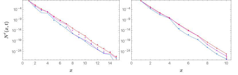
Figure S2: Quantitative match with perturbation theory: Domain wall profile components $N^{\prime}(x,t)$ for small $a$, $a=0.06$ (left), $a=0.02$ (right), and $\tau=(\sqrt{5}-1)\pi/2$, and three different $t=25$ (red), $t=35$ (magenta), $t=45$ (blue). Bullet denote leading order perturbative formula (22).

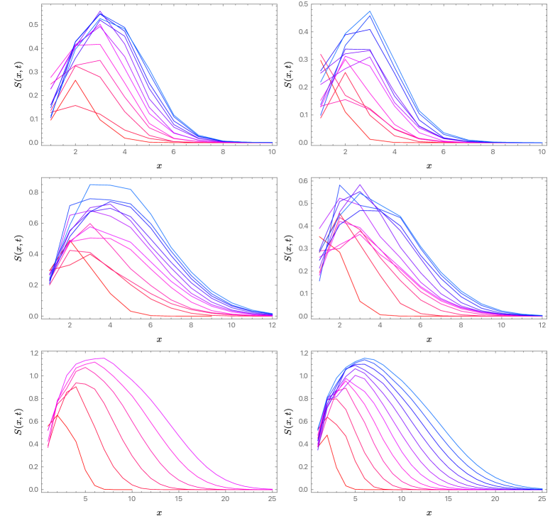
Figure S3: Entanglement entropy dynamics $S(x,t)$, for $t=20,30,\ldots,120$ (red to blue curves) approaching the localisation transition for smaller values of $\tau$, specifically $\tau=(\sqrt{5}-1)\pi/8$ (left column panels) and $\tau=(\sqrt{5}-1)\pi/16$ (right column panels), and three different values of $a$, $a=0.6$ (top row panels), $a=0.8$ (middle row panels), $a=1.0$ (bottom row panels). Note that only in the bottom row panels we see clearly linear growth of entanglement entropies, signalling ergodic dynamics, so the transition should appear for $0.8<a_{c}<1.0$ for both values of $\tau$ (compare against the phase diagram in the main text).

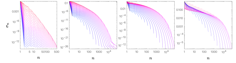
Figure S4: Entanglement (Schmidt) spectra: We show Schmidt spectra for $\tau=(\sqrt{5}-1)\pi/2$, $t=36$, and different $a=0.2,0.3,0.5,1.0$ (left to right panels). Red to blue curves correspond to cuts from $x=2,3,\ldots,35$.

Appendix E Ladder vs brickwall cicruit

In Fig. S5 we show explicitly the similarity transformation, as a piece of quantum circuit, between the brick-wall and the ladder propagators of the Floquet Qantum East model.

$$\leavevmode\hbox to47.7pt{\vbox to55.37pt{\text{[drawing]}}}=\leavevmode\hbox to47.7pt{\vbox to50.59pt{\text{[drawing]}}}$$

Figure S5: Similarity transformation $\mathbb{S}$ (shaded region) between the $\mathbb{U}$ and $\mathbb{U}_{\ell}$: $\mathbb{S}\mathbb{U}=\mathbb{U}_{\ell}\mathbb{S}$.

Appendix F Additional data for IPR from exact diagonalization of finite systems

In the main text we showed how IPR scales with $L$, and with $\tau$ and $a$. It is also illustrative to look at the scaling with $a$ for a fixed $\tau$ and a few different values of $L$, which we report in Fig. S6. We see that there is an almost $L$ independent part where the IPR decreases significantly with increasing $a$. This could be interpreted as the region where the localisation length $\xi$ increases with increasing $a$, resulting in decreasing IPR $\sim 2^{-\xi}$. When $\xi$ increases beyond $L$, we see $L$ dependent values of IPR.

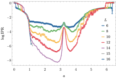
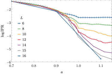
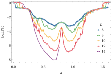
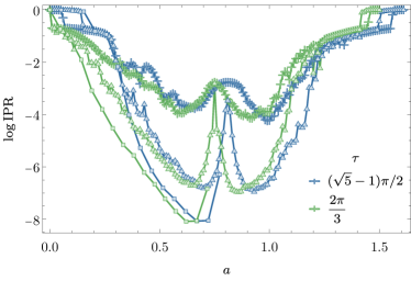
Figure S6: (Top) Logarithm of IPR versus $a$ at $\tau=(\sqrt{5}-1)\pi/8$ for different system sizes $L$. We see the the transition close to $a=1$. On the right we zoom on the collapse of data for different system sizes close to transition. (Bottom left) Same as above with $\tau=(\sqrt{5}-1)\pi/2$. (Bottom right) A comparison between irrational $\tau=(\sqrt{5}-1)\pi/2\sim 1.94161$ (blue) and rational $\tau=\frac{2\pi}{3}\sim 2.0944$ (green) for system sizes $L=8,12,14$ (cross, triangle, square). Even thought these $\tau$ are close, the transition of the irrational one is close to $a=0.3$ versus the rational one shows IPR shrinking with system size for much smaller $a$.

References

Basko et al. [2006]D. Basko, I. Aleiner, and B. Altshuler, Metal-insulator transition in a weakly
interacting many-electron system with localized single-particle states, Annals of
Physics 321, 1126
(2006).
Serbyn et al. [2013]M. Serbyn, Z. Papić, and D. A. Abanin, Local conservation laws and the structure of the many-body
localized states, Phys. Rev. Lett. 111, 127201 (2013).
Ros et al. [2015]V. Ros, M. Müller, and A. Scardicchio, Integrals of motion in the many-body
localized phase, Nuclear Physics B 891, 420 (2015).
Thiery et al. [2018]T. Thiery, F. m. c. Huveneers, M. Müller, and W. De Roeck, Many-body delocalization
as a quantum avalanche, Phys. Rev. Lett. 121, 140601 (2018).
Abanin et al. [2019]D. A. Abanin, E. Altman,
I. Bloch, and M. Serbyn, Colloquium: Many-body localization, thermalization, and
entanglement, Rev. Mod. Phys. 91, 021001 (2019).
Šuntajs et al. [2020]J. Šuntajs, J. Bonča, T. Prosen, and L. Vidmar, Quantum chaos challenges many-body
localization, Phys. Rev. E 102, 062144 (2020).
Abanin et al. [2021]D. Abanin, J. Bardarson,
G. De Tomasi, S. Gopalakrishnan, V. Khemani, S. Parameswaran, F. Pollmann, A. Potter, M. Serbyn, and R. Vasseur, Distinguishing localization from chaos: Challenges in finite-size systems, Annals of Physics 427, 168415 (2021).
Sels and Polkovnikov [2021]D. Sels and A. Polkovnikov, Dynamical obstruction
to localization in a disordered spin chain, Phys. Rev. E 104, 054105 (2021).
van Horssen et al. [2015]M. van
Horssen, E. Levi, and J. P. Garrahan, Dynamics of many-body localization in
a translation-invariant quantum glass model, Phys. Rev. B 92, 100305 (2015).
Crowley [2017]P. Crowley, Entanglement and thermalization in
many body quantum systems, Ph.D. thesis, UCL (University College London) (2017).
Brighi et al. [2022]P. Brighi, M. Ljubotina, and M. Serbyn, Hilbert space fragmentation and slow
dynamics in particle-conserving quantum east models (2022), arXiv:2210.15607
[quant-ph] .
Geissler and Garrahan [2022]A. Geissler and J. P. Garrahan, Slow dynamics and
non-ergodicity of the bosonic quantum east model in the semiclassical limit
(2022), arXiv:2209.06963 [cond-mat.stat-mech] .
Klobas et al. [2023]K. Klobas, C. De Fazio, and J. P. Garrahan, Exact ”hydrophobicity” in deterministic
circuits: dynamical fluctuations in the floquet-east model (2023), arXiv:2305.07423
[cond-mat.stat-mech] .
Valencia-Tortora et al. [2022]R. J. Valencia-Tortora, N. Pancotti, and J. Marino, Kinetically constrained
quantum dynamics in superconducting circuits, PRX Quantum 3, 10.1103/prxquantum.3.020346 (2022).
Pancotti et al. [2020]N. Pancotti, G. Giudice,
J. I. Cirac, J. P. Garrahan, and M. C. Bañuls, Quantum east model: Localization, nonthermal
eigenstates, and slow dynamics, Phys. Rev. X 10, 021051 (2020).
Lanyon et al. [2011]B. P. Lanyon, C. Hempel,
D. Nigg, M. Müller, R. Gerritsma, F. Zähringer, P. Schindler, J. T. Barreiro, M. Rambach, G. Kirchmair, et al., Universal digital quantum simulation with trapped ions, Science 334, 57 (2011).
Barreiro et al. [2011]J. T. Barreiro, M. Müller, P. Schindler, D. Nigg,
T. Monz, M. Chwalla, M. Hennrich, C. F. Roos, P. Zoller, and R. Blatt, An open-system quantum
simulator with trapped ions, Nature 470, 486 (2011).
Blatt and Roos [2012]R. Blatt and C. F. Roos, Quantum simulations with
trapped ions, Nature Physics 8, 277 (2012).
Monroe et al. [2021]C. Monroe, W. C. Campbell, L.-M. Duan,
Z.-X. Gong, A. V. Gorshkov, P. W. Hess, R. Islam, K. Kim, N. M. Linke, G. Pagano, P. Richerme,
C. Senko, and N. Y. Yao, Programmable quantum simulations of spin systems with
trapped ions, Rev. Mod. Phys. 93, 025001 (2021).
Salathé et al. [2015]Y. Salathé, M. Mondal,
M. Oppliger, J. Heinsoo, P. Kurpiers, A. Potočnik, A. Mezzacapo, U. Las Heras, L. Lamata,
E. Solano, S. Filipp, and A. Wallraff, Digital quantum simulation of spin models with circuit quantum
electrodynamics, Phys. Rev. X 5, 021027 (2015).
Barends et al. [2015]R. Barends, L. Lamata,
J. Kelly, L. García-Álvarez,
A. G. Fowler, A. Megrant, E. Jeffrey, T. C. White, D. Sank, J. Y. Mutus, et al., Digital quantum simulation of fermionic models with a superconducting
circuit, Nature Comm. 6, 1 (2015).
Langford et al. [2017]N. K. Langford, R. Sagastizabal, M. Kounalakis, C. Dickel,
A. Bruno, F. Luthi, D. J. Thoen, A. Endo, and L. DiCarlo, Experimentally simulating the dynamics of quantum light and matter
at deep-strong coupling, Nature Comm. 8, 1 (2017).
Kjaergaard et al. [2020]M. Kjaergaard, M. E. Schwartz, J. Braumüller, P. Krantz, J. I.-J. Wang,
S. Gustavsson, and W. D. Oliver, Superconducting qubits: Current state of play, Annual Rev. Cond. Matt. Phys. 11, 369 (2020).
Bravyi et al. [2022]S. Bravyi, O. Dial,
J. M. Gambetta, D. Gil, and Z. Nazario, The future of quantum computing with superconducting qubits, J. Appl. Phys. 132, 160902 (2022).
Schollwöck [2011]U. Schollwöck, The density-matrix
renormalization group in the age of matrix product states, Ann. Phys. 326, 96 (2011).
Cirac et al. [2021]J. I. Cirac, D. Pérez-García, N. Schuch, and F. Verstraete, Matrix product states
and projected entangled pair states: Concepts, symmetries, theorems, Rev. Mod. Phys. 93, 045003 (2021).
Suzuki [1991]M. Suzuki, General theory of fractal
path integrals with applications to many-body theories and statistical
physics, J. Math. Phys. 32, 400 (1991).
Note [1]See the Supplemental Material that contains: (i) A
perturbative analysis of . (ii) A perturbative analysis of
in the Trotter limit. (iii) A self-contained discussion of our TEBD
algorithm. (iv) Further TEBD data. (v) Further finite-volume
data.
Arnold [1961]V. I. Arnold, Small denominators. i.
mapping the circle onto itself, Izv. Akad. Nauk SSSR Ser. Mat 25, 21 (1961).