Geometric Pooling: maintaining more useful information

Abstract

Graph Pooling technology plays an important role in graph node classification tasks. Sorting pooling technologies maintain large-value units for pooling graphs of varying sizes. However, by analyzing the statistical characteristic of activated units after pooling, we found that a large number of units dropped by sorting pooling are negative-value units that contain useful information and can contribute considerably to the final decision. To maintain more useful information, we proposed a novel pooling technology, called Geometric Pooling (GP), containing the unique node features with negative values by measuring the similarity of all node features. We reveal the effectiveness of GP from the entropy reduction view. The experiments were conducted on TUdatasets to show the effectiveness of GP. The results showed that the proposed GP outperforms the SOTA graph pooling technologies by $1\%$ $\sim$ $5\%$ with fewer parameters.

=-21pt

I Introduction

The graph neural networks (GNNs) [3, 19] have been applied and developed in many domains, such as Biomedicine [6, 9], Semantic Segmentation [14], Pose Estimation [29, 26, 27, 28, 25], and Recommender System [30]. GNNs are able to extract good representations from graph-structured data in non-Euclidean space. Mimicking Convolutional Neural Networks (CNNs), researchers designed GNNs sequentially containing convolutional filters, activation functions, and pooling operators to extract features with non-linearity and invariance. Nevertheless, the typical pooling technology in CNNs, such as max-pooling and average-pooling, requires that the processed data are structured (i.e., the data in a neighborhood are in a strong correlation assumption) and is not suitable for non-Euclidean data. However, the graph-structured data does not satisfy the assumption, and the pooling technology brings the key invariance and increases the receptive field of the whole graph, is very important for GNNs.

Many researchers paid attention to the GNN pooling technologies, which are divided into Global Pooling [34, 1], Topology-based Pooling [5, 4], and Hierarchical Pooling [31, 7]. Global pooling is a simple and effective technology, which is a feature-based technology differing from the topology-based pooling technology. Global pooling methods use manual summation or learning methods to pool all the representations of nodes in each layer. Although global pooling technology does not explicitly consider the topology of the input graph, the previous graph convolutional filter has already considered the topology and implicitly influenced the later pooling. Hence, this paper focuses on the global pooling methods because of its computational efficiency and universality.

Figure 1: We show the main difference between sorting pooling and the proposed GP. Different graphs containing different-number nodes are marked in different colors. The numbers in different nodes represent the sorting indices. For example, the amplitude of the node indexed by 0 is larger than that of indexed by 1. Meanwhile, the color contrast among different nodes in a particular graph means the similarity among different nodes. For the above Sorting Pooling, the maintaining nodes are indexed by 0, 1, and 2 (we assume there are three nodes being maintained). In the below Geometric Pooling, the replaceable nodes are dropped and the nodes carrying unique information of the node are maintained.

However, the existing global pooling methods dropped much useful information due to their decision criteria and the activated function, such as tanh, used in the GNNs. For example, Sorting Pooling [34] maintains the large-value units and drops small-value units by sorting the units. The effectiveness of Sorting Pooling is depended on the assumption that the dropped units contribute little to the final decision. However, due to the activation function, tanh, used in Sorting Pooling, the sorting methods not only drop the small-value units but also the negative-value ones. The negative-value units with large absolute values actually carry considerable information, representing the node and contributing much to the final decision. And unfortunately, tanh cannot be replaced by the positive-value activation functions (such as ReLU, ReLU6) because this leads to a performance drop.

To explore the number of dropped negative-value units and the small-value units, which respectively contribute much and little to the final decision, we counted their number in Fig. 2a. Obviously, the “useless” units accounted for a small proportion of all dropped units, and “useful” units accounted for a larger proportion. The dropped information problem cannot be addressed by a simple absolute sorting pooling because when the number of dropped units is fixed (Seeing [34]), the number of “useless” units is not enough and the useful units are also dropped.

Seeing this, we proposed a novel pooling decision criterion - Geometric Pooling (GP) to maintain more useful information, whether positive-value or negative-value units. Different from the global pooling methods, which drop the units with relatively less contribution, the proposed GP dropped the relatively most replaceable units. Particularly, we used a metric such as Euclidean distance, inner product, cosine similarity [22], and Mahalanobis distance [16], to measure the similarity between different nodes. We used Euclidean distance because of its simplicity and low computation cost. In the graph classification task, we dropped the most replaceable node features. The main difference between sorting pooling and GP is visualized in Fig. 1. By exploring the effectiveness, we found that the proposed GP can be viewed as a sort of regularization method, entropy reduction, such as Label Smoothing [18], Mixup[33], and Cutmix [32]. They alleviate the over-confidence problem, which leads to the over-fitting problem. Dropping the replaceable units maximizes the compressing information rate and improves the representation of the node. We stated the regularization view in Section III-D.

To verify the effectiveness of GP, we used the backbone of DGCNN [34], and used GP to replace the original pooling technology. The evaluated experiments are conducted on the TUdataset [17]. The experimental results show that GP outperforms the SOTA graph pooling methods.

The main contributions of this paper are as follows.

1. We analyzed the units dropped by the existing global pooling technologies and found that many negative-value units with useful information are dropped. Seeing this, this paper proposed a novel pooling decision criterion - Geometric Pooling (GP) to drop the most replaceable units, maintaining more useful information.

2. By exploring the effectiveness, this paper viewed the proposed GP as a regularization method, which smooths the distribution of the outputs and maximizes the compressing information rate, addressing the overfitting problem.

3. Comprehensive evaluated experiments show that GP outperforms the existing deep and kernel-based pooing technologies.

II Related Works

Graph global pooling technologies. Sorting Pooling [34] maintains the large-value units and drops the small-value units. This is similar to the norm-based pruning technologies, which determine the importance of the units by their contributions to the final decision. Furthermore, SAGPooling [15] uses self-attention [23] to mask the features pooled by Sorting Pooling. Different from the Sorting Pooling, gPooling [8] not only uses the sorting indices to select the node features but also the corresponding adjacency matrix. According to the selected adjacency matrix, the topological links between the selected nodes are strengthened, and the unimportant links are dropped.

Entropy reduction. Entropy reduction appear in many regularization methods. The typical one is label smoothing [18]. Label smoothing improves the robustness of the trained network by using soft targets that are a weighted average of the hard targets and the uniform distribution over labels. This is equivalent to the effectiveness of the method which encourages the output distribution away from the distribution of the hard targets. Following label smoothing, many researchers proposed many different modified version, such as Mixup [33], Manifold Mixup [24], CutMix [32], to strengthen the entropy reduction according to different tasks.

Zhang et. al proposed Mixup [33] that used the linear combination of different sample of different classes to augment the training samples, and label smoothing is also used to assign the label to the augmented training sample. Manifold Mixup [24] is modified by Mixup, which randomly augments the feature by the linear combination of different features. CutMix [32] is a regularization method which fuses the advantages of Cutout and Mixup.

The above methods encourage the output distribution far away from the distribution of the hard targets. This alleviates the over-confidence problem of the model output, which results in the over-fitting problem. The proposed GP is based on an argument that the similar features works repetitively for the final decision, and we can drop some of them. This also alleviates the over-confidence problem.

III Methods

In this section, we first set up a typical GNNs model. Then the number distribution of the activated units is analyzed in the Sec. III-B. According to the conclusion of the analysis, we stated the proposed Geometric Pooling (GP) in the Sec. III-C. Finally, we give the effectiveness of GP from the entropy reduction view in Section III-D.

III-A Set Up

A graph neural network consists of four parts: 1) graph convolution layers extract nodes’ local substructure features and define a consistent node ordering; 2) a pooling technology is used to unify the size of nodes and impose invariance on the network; 3) an activation layer, such as tanh, is used to give the non-linearity to the previous layers; 4) One or several linear layers are used to inference the class of the input graph.

$\mathbf{X}=\{\mathbf{x}_{i}\}_{i=0}^{N}$ denotes the input set and $\mathbf{x}_{i}\in\mathcal{R}^{n\times d}$, i.e., the input $\mathbf{x}_{i}$ consists of $n$ nodes and each node is a d-dimensional vector. $\mathbf{Y}=\{\mathbf{y}_{i}\}_{i=0}^{N}$ denotes the predict set. In the graph classification task, $\mathbf{A}\in\mathcal{R}$ is the adjacent matrix. $\mathbf{A}$ is a symmetric 0/1 matrix, and the graph has no self-loops.

Graph convolutional layers. Graph convolutional layers aim at learning a mapping $\mathit{f}:(\mathbf{H}^{(l)},\widetilde{\mathbf{A}})\rightarrow\mathbf{H}^{(l+1)}$, where $\mathbf{H}^{(l)}$ is the activation vector in the $l_{th}$ layer and $\mathbf{H}^{(0)}=\mathbf{X}$. For example, we formulated the graph convolution layers defined in [34]:

$$\mathbf{H}^{(l+1)}=\mathit{\sigma}(\widetilde{\mathbf{D}}^{-1}\widetilde{\mathbf{A}}\mathbf{H}^{(l)}\mathbf{W}^{(l)}),$$ (1)

where $\widetilde{\mathbf{A}}=\mathbf{A}+\mathbf{I}$ is the adjacency matrix with added self-loops, $\widetilde{\mathbf{D}}$ is its diagonal degree matrix with $\widetilde{\mathbf{D}}_{ii}=\sum_{j}\widetilde{\mathbf{A}}$, $\mathbf{W}^{(l)}\in\mathcal{R}^{d_{l}\times d_{l+1}}$ is the trainable graph convolution parameters of the $l_{th}$ layers, and $\mathit{\sigma}$ is a nonlinear activation function. In Eq. 1, $\mathbf{H}^{(l)}\mathbf{W}^{(l)}$ is a linear transformation for the input $\mathbf{H}^{(l)}$ to extract the key information. Then $\widetilde{\mathbf{A}}\mathbf{H}^{(l)}\mathbf{W}^{(l)}$ used self-looped adjacency matrix to propagate node information to neighboring nodes along with the topological structure. Finally, $\widetilde{\mathbf{D}}^{-1}$ is used to keep a fixed feature scale after graph convolution.

Pooling. Global pooling operator of GNNs can be viewed as a selected operator, which selects the representative node features and impose invariance on the model. The global pooling operator considers the importance of each node feature.

Activation function. A typical activation function is the hyperbolic tangent function (tanh):

$$z=\frac{e^{x}-e^{-x}}{e^{x}+e^{-x}}.$$

III-B Analysis of the Number Distribution

We analyzed two sorts of sorting pooling: DGCNN [34] and Filter Norm Sorting [15]. DGCNN concatenates the features of different graph convolutional layers to represent the whole graph. In DGCNN, the contributions of the units are determined by the values of the units in the last graph convolutional layer, i.e., DGCNN drops the node features with small-value units in the last graph convolutional layer. However, the contribution of a particular node ought to be jointly determined by all features of this node, not only the units in the last layer. This dropped a lot of representative node features (useful information).

(a) sorting pooling

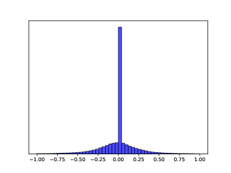
(b) geometric pooling

Figure 2: The counting histograms of sorting pooling and GP technologies. In (a), the units are dropped by sorting pooling; in (b), the units are dropped by geometric distance between the node features.

We counted the values of dropped units in Fig. 2. We counted the dropped unit on D&D dataset, with setting $k$ to 20. As shown in Fig. 2 (a), sorting pooling drops a large number of negative-value units but with large absolute values. Differently, the proposed GP drops the node features sharing large similarity with other node features. Obviously, in Fig. 2 (b), the dropped units are concentrated around zero. In addition, the other dropped units distribute uniformly, i.e., replaceable units are dropped. Consequently, more useful information are maintained.

III-C Geometric Pooling

To get rid of the constraints in the analysis of Sec. III-B, we proposed a novel pooling decision criterion - Geometric Pooling (GP). GP used the similarity between different node features to judge the importance of the node. The whole pooling process is formulated as follows.

We use the feature concatenation method in DGCNN [34] as an example, i.e., the input features of a graph are the concatenation of the output different graph convolution layers, denoted as $\mathbf{H}^{0:L}\in\mathcal{R}^{n\times d^{\prime}}$, where $n$ is the node number of the graph, $d^{\prime}=\sum_{l=0}^{L}d_{l}$, and $L$ is layer number of the whole network. $\mathbf{H}^{0:L}$ consists of $\mathbf{H}^{0:L}_{j}\in\mathcal{R}^{d^{\prime}}(j=1,\ldots,n)$, which denotes the concatenated feature of each node. Then, the similarity (distance) between different node features is computed as follows.

$$\mathbf{S}_{j}=\sum_{i=1}^{n}\|\mathbf{H}^{0:L}_{i}-\mathbf{H}^{0:L}_{j}\|,$$ (2)

where $\mathbf{S}=\{\mathbf{S}_{j}\}_{j=1}^{n}$ denotes the similarity vector of all nodes, and $\|\cdot\|$ denotes the metric used to measure the similarity.

According to $\mathbf{S}$, we sorted the $\{\mathbf{S}_{j}\}_{j=1}^{n}$ in Eq. 2 to get the node features with least similarity:

$$\mathbf{Idx}=Topk(\{\mathbf{S}_{j}\}_{j=1}^{n}).$$ (3)

In Eq. 3, $Topk$ is a operator to select the index of the top-k minimal similarity and the selected indices are saved in $\mathbf{Idx}$. $k$ is a hyper-parameter, which means the number of maintaining node features, to make sure the node number of graphs be same. By $\mathbf{Idx}$, we maintain the node features with the index in $\mathbf{Idx}$. The whole pooling process is stated in Alg. 1.

Algorithm 1 Geometric Pooling

1:k - the number of maintaining nodes

2:Input: $\mathbf{H}^{0:L}=\{\mathbf{H}^{0:L}_{j}\}_{j=1}^{n}$

3:for $1\leq j\leq n$ do

4:     Compute $\mathbf{S}_{j}$ by Eq. 2

5:end for

6:Sort $\mathbf{S}=\{\mathbf{S}_{j}\}_{j=1}^{n}$

7:Compute $\mathbf{Idx}$ by Eq. 3

8:Select the node feature with index in $\mathbf{Idx}$

9:Output: $\{\mathbf{H}^{0:L}_{k}\}_{k\in\mathbf{Idx}}$

III-D Entropy Reduction: distribution drag

The typical convolutional neural networks gradually strengthen the influence of the training samples, i.e., the distribution of output logits is forced far away from the initial uniform distribution. We visualized this process in Fig. 3.

Figure 3: We explain the effectiveness of GP from the output distribution drag view. Typically, common cross entropy loss singly encourage the output distribution close to the distribution of the ground truth in one-hot manner. This results to an over-fitting problem. By GP, the output distribution is encouraged to be close to the uniform distribution, i.e., it is punished to be far away from the ground truth.

To state the problem, we first give the formulation of the typical loss function - Cross Entropy Loss:

$$\mathcal{L}_{CE}=\sum_{\mathbf{x}_{i}}\mathbf{y}_{i}\log\frac{1}{\mathbf{q}(\mathbf{x}_{i})}=-\sum_{\mathbf{x}_{i}}\mathbf{y}_{i}\log\mathbf{q}(\mathbf{x}_{i}),$$ (4)

where $\mathbf{x}_{i}$ is the training sample; $\mathbf{p}(\mathbf{x}_{i})$ denotes the output of the model; $\mathbf{y}_{i}$ is the label of $\mathbf{x}_{i}$. When $\mathcal{L}_{CE}$ decreases, the distribution of $\mathbf{y}_{i}$ is pulled to be close to $\mathbf{p}(\mathbf{x}_{i})$, which is in a one-hot manner. The one-hot label is an extreme probability formulation that is far away from the uniform distribution.

Although the one-hot label is the target of the task, a lot of regularization research shows that just pulling the distribution close to the one-hot distribution results in an over-fitting problem. For example, Miller [18] proposed that the effectiveness of Label Smoothing results from the distribution drag. Particularly, the one-hot label is modified to a probability form:

$$[0,0,1,0,0]\rightarrow[0.05,0.05,0.8,0.05,0.05].$$

Obviously, $\mathbf{q}(\mathbf{x}_{i})$ is enforced to be close to the uniform distribution. Label Smoothing effectively strengthens the robustness by alleviating the too-high confidence problem at the training stage, i.e., the over-fitting problem [12].

Many similar units filtered by the convolutional kernels jointly output the final decision of the too-high confidence [11]. Hence dropping the units of high similarity alleviates the too-high confidence problem. Except for the pooling operator, the regularization effectiveness of the proposed GP can be viewed as a penalty term:

$$\mathbf{L}=\mathbf{L}_{CE}+\mathbf{L}_{ana}=-\sum_{\mathbf{x}_{i}}\left[\mathbf{y}_{i}\log\mathbf{q}(\mathbf{x}_{i})+\lambda\cdot D_{KL}(\mathbf{U}_{[0,C]}\|\mathbf{q}(\mathbf{x}_{i}))\right],$$ (5)

where $D_{KL}(\cdot\|\cdot)$ is a Kullback-Leibler divergence; $\lambda$ is the scaling factor; $C$ is the class number of the task. We give the $D_{KL}(\mathbf{U}_{[0,C]}\|\mathbf{q}(\mathbf{x}_{i}))$ as follows.

$$\begin{split}D_{KL}(\mathbf{U}_{[0,C]}\|\mathbf{q}(\mathbf{x}_{i}))&=-\mathbf{U}_{[0,C]}\log\frac{\mathbf{q}(\mathbf{x}_{i})}{\mathbf{U}_{[0,C]}}\\ &=\frac{1}{C}\log\frac{1}{C}-\frac{1}{C}\log\mathbf{q}(\mathbf{x}_{i})\end{split},$$ (6)

where $\frac{1}{C}\log\frac{1}{C}$ is the negative entropy of the uniform distribution $\mathbf{U}_{[0,C]}$ and $-\frac{1}{C}\log\mathbf{q}(\mathbf{x}_{i})$ is the cross entropy between $\mathbf{U}_{[0,C]}$ and $\mathbf{q}(\mathbf{x}_{i})$. $\frac{1}{C}\log\frac{1}{C}$ is a constant in a particular task. When $-\frac{1}{C}\log\mathbf{q}(\mathbf{x}_{i})$ decreases, the output is enforced to be close to $\mathbf{U}_{[0,C]}$, and hence the over-fitting problem is alleviated. To clearly show the distribution drag, we visualized the distribution variation of the vanilla training in the above row and the proposed GP in the below row.

IV Experiments

To show the effectiveness of the proposed GP, we embedded GP in different methods to replace the original pooling technologies on the typical Graph classification dataset - TUdataset.

IV-A Set Up

Datasets. TUdataset consists of too many sub-datasets. Hence we chose MUTAG, PTC, NCI1, PROTEINS, D&D, COLLAB, IMDB-B, and IMDB-M to evaluate the performance. Most chosen sub-datasets contain graphs of two categories, except for COLLAB and IMDB-M, which contain graphs of three categories. The detailed information of the sub-datasets is given in Table I.

TABLE I: The dataset description.

Dataset	MUTAG	PTC	NCI1	PROTEINS
#Graphs	188	344	4,110	1,113
#Classes	2	2	2	2
#Node Attr.	8	19	38	5
Dataset	D&D	COLLAB	IMDB-B	IMDB-M
#Graphs	1,178	5,000	1,000	1,500
#Classes	2	3	2	3
#Node Attr.	90	1	1	1

Comparison methods. We compare the proposed GP with sort pooling in DGCNN [34], SAGPooling [15], DiffPooling [31], and GRAPHSAGE [10] to show GP’s effectiveness. Also, several kernel-based algorithms are compared, including GRAPHLET [21], Shortest-Path [2], Weisfeiler-Lehman kernel (WL) [20], and Weisfeiler-Lehman Optimal Assignment Kernel (WL-OA) [13].

Model Configuration. We used five Graph Convolutional layers to extract different-level features of the graph and a GP layer is used to obtain the salient features and make each graph share the same node number and the same node feature number. The hyper-parameter $k$ in Eq. 3 is varying for different datasets. We set the $k$ such that 60% graphs have nodes more than $k$. For fair evaluation, we used a single network structure on all datasets, and ran GP using exactly the same folds as used in graph kernels in all the 100 runs of each dataset.

IV-B Comparison with deep approaches

As given in Table II, the results of the compared deep approaches show the effectiveness of the proposed GP and its variation – GP-mixed. GP-mixed first used sort pooling [34] to drop some units contributing little to the final decision And then GP is used to drop the replaceable units.

TABLE II: The performance comparison among different deep approaches. The top two test classification accuracy on each dataset is in bold.

Methods	Datasets
	MUTAG	PTC	NCI1	PROTEINS
DGCNN	85.83	58.59	74.44	75.54
GRAPHSAGE	–	–	–	70.48
SAGPooling	–	–	74.06	70.04
DiffPooing	–	–	–	76.25
GP	86.10	61.30	75.80	77.10
GP-mixed	86.44	61.86	76.29	77.64
	D&D	COLLAB	IMDB-B	IMDB-M
DGCNN	79.37	73.76	71.50	46.47
GRAPHSAGE	75.42	68.25	68.80	47.6
SAGPooling	76.19	69.47	–	–
DiffPooing	79.64	75.48	–	–
GP	80.21	74.63	72.20	47.89
GP-mixed	80.28	75.50	72.68	48.32

In Table II, we give several state-of-the-art GNNs pooling performance. For example, on D&D, the proposed GP outperforms DGCNN and SAGPooling by 0.84% and 4.02%, respectively. On COLLAB, GP outperforms DGCNN by 0.87%. Although GP underperforms DiffPooling, GP-mixed slightly outperforms DiffPooling. In general, the proposed GP outperforms the SOTA deep approaches by 0.7% $\sim$ 5.05%.

IV-C Comparison with kernel-based approaches

Kernel-based approaches are also compared. As shown in Table III, the proposed GP and its variant outperform the kernel-based approaches on most evaluation datasets. For example, GP-mixed outperforms the compared kernel-based approaches by 1.21% $\sim$ 4.73% on PROTEINS. Unfortunately, on COLLAB, GP and GP-mixed underperform WL and WL-OA.

TABLE III: The performance comparison between GP and kernel-based approaches. The top two test classification accuracy on each dataset is in bold.

Methods	Datasets
	MUTAG	PTC	NCI1	PROTEINS
GRAPHLET	85.7	54.7	76.20	72.91
SHORTEST-PATH	83.15	–	–	76.43
WL	84.11	57.97	84.46	73.76
WL-OA	84.50	–	–	75.26
GP	86.10	61.30	75.80	77.10
GP-mixed	86.44	61.86	76.29	77.64
	D&D	COLLAB	IMDB-B	IMDB-M
GRAPHLET	74.85	64.66	–	–
SHORTEST-PATH	78.86	59.10	–	–
WL	74.02	78.61	71.26	46.52
WL-OA	79.04	80.74	–	–
GP	80.21	74.63	72.20	47.89
GP-mixed	80.28	75.50	72.68	48.32

IV-D Comparison on the computation cost

To show the simplification of the proposed GP, we also compute the computation cost of the compared deep approaches.

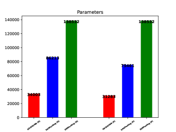
Figure 4: Parameter comparison. We give the parameters of different deep approaches on two datasets: D&D and PROTEINS. For example, let GP/DGCNN (D) denote the parameter amount of the proposed GP and DGCNN on D&D dataset. Also, SAGPooling (P) denotes the parameter amount of SAGPooling on PROTEINS dataset. The numbers on the colored bars mean the exact parameter number.

As shown in Fig. 4, the red bars, which mean the parameter amount of the proposed GP, are far less than that of SAGPooling and DiffPooling approaches. On D&D, the parameter amount of GP accounts for 39.44% of SAGPooling and 24.55% of DiffPooling. This shows the computation efficiency of the proposed GP.

V Conclusion

In the work, we proposed a novel graph pooling technology based on the geometric distance between different node features, called Geometric Pooling (GP). The proposed GP maintains more useful information, which is dropped by other global graph pooling technologies. In addition, the replaceable feature drop brings the entropy reduction, which encourages the output distribution away from the hard targets. This alleviates the over-confidence problem and hence address the over-fitting problem.

References

- [1] Order matters: Sequence to sequence for sets. In International Conference on Learning Representation., 2016.
- [2] K.M. Borgwardt and H.P. Kriegel. Shortest-path kernels on graphs. In Fifth IEEE International Conference on Data Mining (ICDM’05), pages 8 pp.–, 2005.
- [3] Michael M. Bronstein, Joan Bruna, Yann LeCun, Arthur Szlam, and Pierre Vandergheynst. Geometric deep learning: Going beyond euclidean data. IEEE Signal Processing Magazine, 34(4):18–42, 2017.
- [4] Michaël Defferrard, Xavier Bresson, and Pierre Vandergheynst. Convolutional neural networks on graphs with fast localized spectral filtering. In Advances in Neural Information Processing Systems, 2016.
- [5] Inderjit S. Dhillon, Yuqiang Guan, and Brian Kulis. Weighted graph cuts without eigenvectors: A multilevel approach. IEEE Trans. Pattern Anal. Mach. Intell., 29(11):1944–1957, 2007.
- [6] David K Duvenaud, Dougal Maclaurin, Jorge Iparraguirre, Rafael Bombarell, Timothy Hirzel, Alan Aspuru-Guzik, and Ryan P Adams. Convolutional networks on graphs for learning molecular fingerprints. In C. Cortes, N. Lawrence, D. Lee, M. Sugiyama, and R. Garnett, editors, Advances in Neural Information Processing Systems, volume 28. Curran Associates, Inc., 2015.
- [7] Hongyang Gao and Shuiwang Ji. Graph u-net, 2019.
- [8] Hongyang Gao and Shuiwang Ji. Graph u-nets. In Kamalika Chaudhuri and Ruslan Salakhutdinov, editors, Proceedings of the 36th International Conference on Machine Learning, volume 97 of Proceedings of Machine Learning Research, pages 2083–2092. PMLR, 09–15 Jun 2019.
- [9] Justin Gilmer, Samuel S. Schoenholz, Patrick F. Riley, Oriol Vinyals, and George E. Dahl. Neural message passing for quantum chemistry. In Proceedings of the 34th International Conference on Machine Learning - Volume 70, ICML’17, page 1263–1272. JMLR.org, 2017.
- [10] Will Hamilton, Zhitao Ying, and Jure Leskovec. Inductive representation learning on large graphs. In Advances in Neural Information Processing Systems, volume 30, 2017.
- [11] Yang He, Ping Liu, Ziwei Wang, and et al. Filter pruning via geometric medianfor deep convolutional neural networks acceleration. In IEEE Conference on Computer Vision and Pattern Recognition, 2019.
- [12] Matthias Hein, Maksym Andriushchenko, and Julian Bitterwolf. Why relu networks yield high-confidence predictions far away from the training data and how to mitigate the problem. In IEEE Conference on Computer Vision and Pattern Recognition, 2019.
- [13] Nils Kriege, P.-L Giscard, and Richard Wilson. On valid optimal assignment kernels and applications to graph classification. In Advances in Neural Information Processing Systems, pages 1615–1623, 06 2016.
- [14] Loic Landrieu and Martin Simonovski. Large-scale point cloud semantic segmentation with superpoint graphs. In CVPR, 2018.
- [15] Junhyun Lee, Inyeop Lee, and Jaewoo Kang. Self-attention graph pooling. In Proceedings of the 36th International Conference on Machine Learning, 09–15 Jun 2019.
- [16] G. Mclachlan. Mahalanobis distance. Resonance, 4:20–26, 06 1999.
- [17] Christopher Morris, Nils M. Kriege, Franka Bause, Kristian Kersting, Petra Mutzel, and Marion Neumann. Tudataset: A collection of benchmark datasets for learning with graphs. In ICML 2020 Workshop on Graph Representation Learning and Beyond (GRL+ 2020), 2020.
- [18] Rafael Müller, Simon Kornblith, and Geoffrey E. Hinton. When does label smoothing help? In NeurIPS, 2019.
- [19] Franco Scarselli, Marco Gori, Ah Chung Tsoi, Markus Hagenbuchner, and Gabriele Monfardini. The graph neural network model. IEEE Transactions on Neural Networks, 20(1):61–80, 2009.
- [20] Nino Shervashidze, Pascal Schweitzer, Erik Jan van Leeuwen, Kurt Mehlhorn, and Karsten M. Borgwardt. Weisfeiler-lehman graph kernels. Journal of Machine Learning Research, 12(77):2539–2561, 2011.
- [21] Nino Shervashidze, SVN Vishwanathan, Tobias Petri, Kurt Mehlhorn, and Karsten Borgwardt. Efficient graphlet kernels for large graph comparison. In Proceedings of the Twelth International Conference on Artificial Intelligence and Statistics, volume 5 of Proceedings of Machine Learning Research, pages 488–495, 2009.
- [22] Pang-Ning Tan, Michael Steinbach, Anuj Karpatne, and Vipin Kumar. Introduction to Data Mining (2nd Edition). Pearson, 2nd edition, 2018.
- [23] Ashish Vaswani, Noam Shazeer, Niki Parmar, Jakob Uszkoreit, Llion Jones, Aidan N Gomez, Ł ukasz Kaiser, and Illia Polosukhin. Attention is all you need. In Advances in Neural Information Processing Systems, volume 30, 2017.
- [24] Vikas Verma, Alex Lamb, Christopher Beckham, Amir Najafi, Ioannis Mitliagkas, David Lopez-Paz, and Yoshua Bengio. Manifold mixup: Better representations by interpolating hidden states. In Kamalika Chaudhuri and Ruslan Salakhutdinov, editors, Proceedings of the 36th International Conference on Machine Learning, volume 97 of Proceedings of Machine Learning Research, pages 6438–6447. PMLR, 09–15 Jun 2019.
- [25] Yabo Xiao, Kai Su, Xiaojuan Wang, Dongdong Yu, Lei Jin, Mingshu He, and Zehuan Yuan. Querypose: Sparse multi-person pose regression via spatial-aware part-level query. arXiv preprint arXiv:2212.07855, 2022.
- [26] Yabo Xiao, Xiao Juan Wang, Dongdong Yu, Guoli Wang, Qian Zhang, and HE Mingshu. Adaptivepose: Human parts as adaptive points. In Proceedings of the AAAI Conference on Artificial Intelligence, volume 36, pages 2813–2821, 2022.
- [27] Yabo Xiao, Xiaojuan Wang, Dongdong Yu, Kai Su, Lei Jin, Mei Song, Shuicheng Yan, and Jian Zhao. Adaptivepose++: A powerful single-stage network for multi-person pose regression. arXiv preprint arXiv:2210.04014, 2022.
- [28] Yabo Xiao, Dongdong Yu, Xiao Juan Wang, Lei Jin, Guoli Wang, and Qian Zhang. Learning quality-aware representation for multi-person pose regression. In Proceedings of the AAAI Conference on Artificial Intelligence, volume 36, pages 2822–2830, 2022.
- [29] Yabo Xiao, Dongdong Yu, Xiaojuan Wang, Tianqi Lv, Yiqi Fan, and Lingrui Wu. Spcnet: spatial preserve and content-aware network for human pose estimation. arXiv preprint arXiv:2004.05834, 2020.
- [30] Rex Ying, Ruining He, Kaifeng Chen, Pong Eksombatchai, William L. Hamilton, and Jure Leskovec. Graph convolutional neural networks for web-scale recommender systems. In Yike Guo and Faisal Farooq, editors, Proceedings of the 24th ACM SIGKDD International Conference on Knowledge Discovery & Data Mining, KDD 2018, London, UK, August 19-23, 2018, pages 974–983. ACM, 2018.
- [31] Rex Ying, Jiaxuan You, Christopher Morris, Xiang Ren, William L. Hamilton, and Jure Leskovec. Hierarchical graph representation learning with differentiable pooling. In Proceedings of the 32nd International Conference on Neural Information Processing Systems, NIPS’18, page 4805–4815, Red Hook, NY, USA, 2018. Curran Associates Inc.
- [32] Sangdoo Yun, Dongyoon Han, Seong Joon Oh, Sanghyuk Chun, Junsuk Choe, and Youngjoon Yoo. Cutmix: Regularization strategy to train strong classifiers with localizable features. In International Conference on Computer Vision (ICCV), 2019.
- [33] Hongyi Zhang, Moustapha Cisse, Yann N. Dauphin, and David Lopez-Paz. mixup: Beyond empirical risk minimization. In International Conference on Learning Representations, 2018.
- [34] Muhan Zhang, Zhicheng Cui, Marion Neumann, and Yixin Chen. An end-to-end deep learning architecture for graph classification. In Proceedings of the Thirty-Second AAAI Conference on Artificial Intelligence and Thirtieth Innovative Applications of Artificial Intelligence Conference and Eighth AAAI Symposium on Educational Advances in Artificial Intelligence, AAAI’18/IAAI’18/EAAI’18. AAAI Press, 2018.