Coverage Performance of UAV-powered Sensors for Energy-neutral Networks with Recharging Stations
Oktay Cetinkaya1    Mustafa Ozger2    David De Roure1

Abstract

The projected number of Internet of Things (IoT) sensors makes battery maintenance a challenging task. Although battery-less IoT is technologically viable, the sensors should be somehow energized, either locally or remotely. Unmanned aerial vehicles (UAVs) can respond to this quest via wireless power transfer (WPT). However, to achieve energy neutrality across the IoT networks and thus mitigate the maintenance issues, the UAVs providing energy and connectivity to IoT sensors must be supplied by recharging stations having multi-source energy harvesting (EH) capability. Yet, as these sensors rely solely on UAV-transferred power, the absence of UAVs causes sensor outages and hence loss of coverage when they visit recharging stations for battery replenishment. Hence, besides the UAV parameters (e.g., battery size and velocity), recharging duration and station density must be carefully determined to avoid these outages. To address that, this paper uses stochastic geometry to derive the coverage probability of UAV-powered sensors. Our analysis sheds light on the fundamental trade-offs and design guidelines for energy-neutral IoT networks with recharging stations in regard to the regulatory organization limitations, practical rectenna and UAV models, and the minimum power requirements of sensors.

I Introduction

Unmanned aerial vehicles (UAVs) are becoming increasingly essential in wireless networks, serving as either mobile users or base stations/access points (APs) [1]. In addition to the numerous value-added services they already provide, UAVs also play a critical role in addressing the battery constraints of the Internet of Things (IoT) through wireless power transfer (WPT) [2]. They are particularly beneficial for networks that rely on a multitude of sensors, which require excessive maintenance, or that operate in hard-to-reach areas, such as rainforests. By offering line-of-sight (LoS) air-to-ground links, UAVs enable highly efficient WPT [3], which, in turn, enables the battery-less operation of sensors deployed on the ground. After delivering the energy required by sensors, UAVs can also collect sensory data by acting as mobile APs, thereby offering an all-in-one solution. In these settings, UAVs govern both energy and data flows with no human supervision for battery maintenance or terrestrial APs for data collection, aiming for a certain level of autonomy in network operation.

Since the primary goal of a WPT-enabled UAV setting is to minimize the battery constraints of sensors, besides the prevailing energy scarcity across the IoT domain, the energy required for UAV operation, including the power transferred to sensors, has to be provisioned within the network. In this way, energy neutrality can be enabled [4], mitigating the challenges mentioned above. One approach for achieving this goal is to replenish UAV batteries via recharging stations having energy harvesting (EH) capability. Here, multiple ambient sources, such as solar and wind power, can be simultaneously exploited [5] to minimize the variance and intermittency in the EH output for assured reliability.

The literature has vast examples of UAV-based service provisioning for IoT devices, including recharging stations. In most cases, the UAVs operate as flying APs [6] to collect sensory data underpinned by terrestrial counterparts. They sometimes deliver power [7] in addition to or aside from AP functionality [8]. The recharging stations are usually deemed to have mains connection, or their source of power is untold [9], both referring to a case with an unlimited energy source, i.e., the total disregard of the energy neutrality objective.

One domain that has been exhaustively studied in the literature is the UAV-assisted IoT networks, in which the UAVs provide coverage to sensors. For example, the authors in [10] optimized the trajectory of a UAV energized by a solar-powered recharging station in consideration of data rate, energy consumption, and fairness of coverage. However, they focused on a single UAV operation without considering the effect of recharging station density, limiting their application potential. Furthermore, the authors in [11] proposed a distributed blockchain-based scheme to enable secure and reliable energy exchange between UAVs and recharging stations. However, they did not consider the energy-neutral operation of their system, leading to an impractical solution. The authors in [12] proposed reinforcement learning algorithms to jointly optimize the velocity and energy replenishment of UAVs that collect data from sensors. Although they enabled efficient transfer learning techniques to decrease the learning time and improve the overall learning process, they did not take energy neutrality into consideration in their setting, similar to other studies.

As discussed in [13] and the references therein, the literature on UAV-assisted sensor coverage mainly focused on various other aspects, such as clustering the sensor nodes for more energy-efficient data collection, different flying modes of UAVs, and joint path planning and resource allocation via graph-theory, optimization, machine learning, etc. Despite the promising findings of these studies, the research must look towards a more pressing and fundamental issue, i.e., how to achieve energy-neutral IoT at the minimal sensor outage, occurring due to recharging station-driven UAV operation. Hence, the following aspects need considerable attention for a more realistic analysis of the coverage performance of sensors, facilitating energy neutrality in the IoT domain: i) effective isotropic radiated power (EIRP) limitations enforced by regulatory organizations; ii) practical rectenna models with non-linear EH behavior; iii) minimum power requirements of sensors; iv) individual duration of each UAV operation; and most importantly, v) a limited source of power for WPT, i.e., the UAVs energized by multi-source EH recharging stations.

The current gap in the research field being highlighted, this work aims to mathematically analyze the coverage probability of sensors powered by multi-source EH recharging stations through UAVs performing WPT with directive antennae. Since the UAVs manage both energy and data flows in the envisioned scenario, no service is available during their trip (towards sensors and recharging stations) and battery replenishment, which refers to an outage or no coverage of sensors. The goal is to maximize the coverage probability by tweaking the crucial design parameters, such as the station density, UAV velocity, battery capacity, and recharging time.

Following the agenda given above, we used stochastic geometry in order to derive a tractable expression for the event of service guaranteeing a certain level of coverage. Our analyses, based on practical rectenna and UAV propulsion models, revealed the non-trivial relationships between the UAV attributes (e.g., availability, velocity, descent altitude, antenna directivity, energy budget, output power, transmission duration, and operating frequency); sensor characteristics (e.g., sensitivity, antenna gain, and power conversion efficiency); medium specifications (e.g., urban, suburban); and application requirements (e.g., minimum reporting frequency). In the end, our study provides an upper bound for the coverage probability of sensors, which can be practically achieved by carefully selecting the design parameters in a UAV-powered energy-neutral application scenario involving EH recharging stations.

The remainder of this paper is organized as follows. We first introduce the system model in Section II, where the event of service, incorporating directivity, UAV propulsion, WPT and rectenna models, and FCC regulations, are formulated. Then, in Section III, we derive the coverage probability of sensors based on stochastic geometry. This is followed by the numerical evaluation of the proposed model in Section IV to reveal the design guidelines that must be followed for the best achievable coverage while meeting application requirements. Finally, Section V discusses future research directions and concludes the paper.

II System Model

As illustrated also in Fig. 1, we envision an energy-neutral network scenario, which comprises: i) recharging stations, ii) UAVs, and iii) battery-less sensors. The UAVs retrieve energy from multi-source EH recharging stations via inductive power transfer, fly towards the sensors, energize them via radio frequency (RF) power transfer, and collect their data. During power transfer and data collection, which refers to service, the UAVs do not move in the 3D space; they just hover at the centers of event areas, i.e., where sensors reside. The sensors become active as soon as they intercept enough power from a UAV. When active, they probe their vicinity for an application-defined parameter, e.g., temperature, humidity, and/or noise level, and notify their respective UAV with their readings. After collecting sensor data, the UAVs fly back to the nearest recharging station to replenish their batteries.

As explained, the UAVs singlehandedly manage energy and data flows within the network in an autonomous manner; there are no other authorized entities, terrestrial APs, energy providers, etc. The service is provided at the centers of event areas, i.e., randomly located circles with radius $r_{\Delta}$, which are modeled as a Poisson point process (PPP). Within each circle, the sensors are uniformly distributed, and finally, the locations of recharging stations are modeled as a PPP $\Phi_{Ch}$ with density $\lambda_{Ch}$. Below, we explain the service in detail.

II-A Service Provisioning

In our envisioned scenario, recharging stations refill the UAV battery with energy that is just enough for i) a round trip to the event area, i.e., travel to its center and descent/ascent to/from it, ii) providing service, and iii) hovering when providing service. During the trip and getting its battery replenished, the UAV cannot provide any service, i.e., it is unavailable.

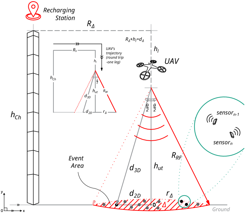
Figure 1: Illustration of the envisioned network scenario.

The definition above confirms that the service is conditioned on the distance between the point where it is provided and the nearest charging station, $d_{\Delta}(=\!R_{\Delta}+h_{l})$. However, only one of $d_{\Delta}$’s components, namely $R_{\Delta}$, changes randomly due to the distribution of recharging stations. Hence, the probability of UAV’s availability, i.e., the event of service $\mathcal{E}$, is conditioned on $R_{\Delta}$, which can be given as:

$$\begin{split}P_{(\mathrm{e|R_{\Delta}})}&=\mathbb{P}(\mathcal{E}|R_{\Delta})\\ &=\frac{t_{PT}+t_{AP}}{t_{PT}+t_{AP}+t_{Ch}+t_{J}},\end{split}$$ (1)

where $t_{PT}$ is the time spent for power transfer, $t_{AP}$ is the time spent for data collection, $t_{Ch}$ is the time spent for recharging the UAV battery, and $t_{J}$ is the time spent for the round trip. Here, each of $t_{J}$, $t_{PT}$, and $t_{AP}$ can be defined as:

$$\begin{aligned} t_{J}&=\frac{2(R_{\Delta}+h_{l})}{V}=\frac{2d_{\Delta}}{V},\\ t_{PT}&=\frac{E_{PT}}{P_{T}},\\ t_{AP}&=\frac{B_{\mathrm{UAV}}-t_{PT}(P_{h}+P_{T})-t_{J}P_{J}}{P_{h}},\end{aligned}$$ (2)

where $P_{J}$ is the power consumption during the trip, $V$ is the UAV’s velocity during the trip, $E_{PT}$ is the energy budget spared for power transfer, $P_{h}$ is the power consumption during hovering at the center of an event area, $P_{T}$ is the transmit power of the UAV, and $B_{\mathrm{UAV}}$ is the energy level of the UAV battery. We should note that the UAV battery might not be fully charged always since it predominately depends on the power transfer rate of the wireless pad, $\xi_{Ch}$, of the recharging station and the time the UAV spends on it, $t_{Ch}$. From (1), we also know that $t_{Ch}$ is inversely proportional to UAV availability since it is on the denominator of the equation, so it should be limited. That is also because the UAV battery has a limited/maximum capacity, $B_{\mathrm{max}}$, so the UAV should not reside on the charging pad beyond when the battery gets fully charged, referring to $t_{Ch}^{sat}$. Note that the saturation time $t_{Ch}^{sat}$ can be achieved sooner or later depending on the charging rate $\xi_{Ch}$ since $B_{\mathrm{max}}$ is fixed. Considering all these, an accurate battery charging model for the UAV can be given as:

$$B_{\mathrm{UAV}}(t_{Ch})=\begin{cases}\xi_{Ch}\cdot t_{Ch},&\leavevmode\nobreak\ t_{Ch}\in[0,t_{Ch}^{sat}],\\ B_{\mathrm{max}},&t_{Ch}\geq t_{Ch}^{sat}.\end{cases}$$ (3)

and finally, by taking the expectation of (1), the service probability of the UAV can be calculated as:

$$P_{\mathrm{e}}=\mathbb{E}_{\Phi_{Ch}}\bigg{[}\frac{t_{PT}+t_{AP}}{t_{PT}+t_{AP}+t_{Ch}+t_{J}}\bigg{]}.$$ (4)

II-B Power Transfer

The UAV performs RF power transfer with a directional antenna having a pencil-beam-like radiation pattern. For such an antenna, i.e. with one major lobe and very negligible minor lobes of the beam, the gain $G_{T}$ can be approximated by:

$$G_{T}=\begin{cases}\approx\!\dfrac{30000}{\theta_{B}^{2}},&\leavevmode\nobreak\ \frac{-\theta_{B}}{2}\leq\varphi\leq\frac{\theta_{B}}{2},\leavevmode\nobreak\ \leavevmode\nobreak\ \leavevmode\nobreak\ \leavevmode\nobreak\ \leavevmode\nobreak\ \text{(major lobe)}\\ \leavevmode\nobreak\ \leavevmode\nobreak\ \leavevmode\nobreak\ \leavevmode\nobreak\ \leavevmode\nobreak\ g(\varphi),&\leavevmode\nobreak\ \leavevmode\nobreak\ \leavevmode\nobreak\ \leavevmode\nobreak\ \leavevmode\nobreak\ \leavevmode\nobreak\ \leavevmode\nobreak\ \text{otherwise},\leavevmode\nobreak\ \leavevmode\nobreak\ \leavevmode\nobreak\ \text{(minor lobes)}\end{cases}$$ (5)

where $\varphi$ is the sector angle, $\theta_{B}$ is the directional antenna half-power beamwidth (HPBW) -both in degrees, $\approx\!30000/\theta_{B}^{2}$ is the maximum gain, and $g(\varphi)$ is the gain outside of the major lobe (including minor lobes), which can be neglected [14]. Note that (5) is for a symmetrical radiation pattern, where the HPBWs in each plane are equal to each other, i.e. $\theta_{1d}\!=\!\theta_{2d}$.

Contrary to expectations, the transmit power of the UAV, $P_{T}$ in (2), cannot be altered casually; it is determined by regulatory organizations, e.g., the Office of Communications (Ofcom) in the UK, the Federal Communications Commission (FCC) in the US. For example, FCC Part 15.247 rules [15] declare that the maximum $P_{T}$ fed into the (in our case, UAV’s) antenna cannot exceed $30$dBm ($1$W) for the industrial, scientific, and medical (ISM) bands, in which the maximum effective isotropic radiated power ($\mathrm{EIRP_{max}}$) is limited to $36$dBm ($4$W). This indicates that increasing $G_{T}$ necessitates a proportional decrease in $P_{T}$, and vice versa, such that the total RF power radiated by the antenna remains the same, i.e., $4$W EIRP, where $\max(P_{T})\!=\!1$W for each case. For directional dispersion, however, there are some exceptions to the $\mathrm{EIRP_{max}}$, details of which can be found in [15].

Here, we should note the following: i) since the antenna size increases with increasing $G_{T}$, the $G_{T}$ vs. $P_{T}$ balance must be maintained regarding what a UAV can physically accommodate, ii) power transfer should be administrated at a low frequency ($f$, preferably sub-GHz), as the power received by sensors ($P_{R}$) is inversely proportional to the square of $f$, i.e., $P_{R}\varpropto 1/f^{2}$, iii) since the UAV has a fixed budget for power transfer ($E_{PT}$), decreasing $P_{T}$ means a longer $t_{PT}$, which may affect the service probability of the UAV -from (1). The lengthened coverage lifetime, $t_{PT}$, despite sounding attractive, will alter the duty cycle of sensors, which cannot be tolerated always due to the certain reporting frequency requirements of IoT applications [16]. Thus, these trade-offs must be carefully considered during the system design to maximize the performance metric defined by the application.

II-C Trip Power Consumption

The rotary-wing type UAVs that we have need fixed power during their trip, which can be approximated as [17]:

$$P_{J}(V)\approx P_{0}\bigg{(}1+\frac{3V^{2}}{U^{2}_{tip}}\bigg{)}+\frac{P_{i}v_{0}}{V}+\frac{1}{2}d_{0}\rho sAV^{3},$$ (6)

where $U^{2}_{tip}$ is the tip speed of the rotor blade, $v_{0}$ is the mean rotor-induced velocity when hovering, $d_{0}$ is the fuselage drag ratio, $\rho$ is the air density, $s$ is the rotor solidity, $A$ is the rotor disc area, and $P_{0}$ and $P_{i}$ are the UAV’s blade profile power and induced power in hovering status, respectively. Here, $P_{h}$ can be defined as the sum of $P_{0}$ and $P_{i}$, i.e.,:

$$P_{h}=\underbrace{\frac{\delta}{8}\rho sA\Omega^{3}R^{3}}_{\text{$\triangleq P_{0}$}}+\underbrace{(1+k)\frac{W^{3/2}}{\sqrt{2\rho A}}}_{\text{$\triangleq P_{i}$}},$$ (7)

where $\Omega$ is the blade angular velocity, $R$ is the rotor radius, $k$ is the incremental correction factor to induced power, and $W$ is the UAV weight. Using the respective values of each parameter given in [17], $P_{J}$ as a function of $V$ is illustrated in Fig. 2(a), which is also used in our calculations.

From (2) and (6), the energy that the UAV needs for a round trip, $E_{J}$, is $t_{J}\,\times\,P_{J}\,=\,\tfrac{2(R_{\Delta}+h_{l})}{V}P_{J}$, where each leg consumes the half, i.e., $E_{J}/2$ for travelling to or from the service point. That is important, as the energy left in $B_{\mathrm{UAV}}$ after providing service must be enough for UAV to make it to the nearest charging station before depleting its battery, i.e., $\!E_{\mathrm{left}}\!\geq\!E_{J}/2$. In our analyses, we evaluate the effect of $V$ in minimizing $E_{J}$, ensuring that the UAV has more resources for service.

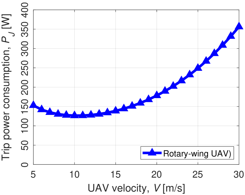
(a)

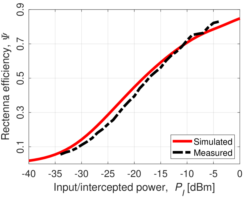
(b)

Figure 2: (a) Trip power consumption, $P_{J}$, vs. UAV velocity, $V$, as modelled in [17]; (b) rectenna efficiency, $\Psi$, as a function of input/intercepted power, $P_{I_{\chi}}$, for the rectenna in [18] ($@f_{c}\!=\!868$MHz).

II-D Sensor Association

We assume that each event area, $\Delta$, is serviced by only one UAV at a time, i.e., each sensor is associated with one UAV hovering at the center of $\Delta$ that the sensor falls into. Otherwise, the sensor has no service, which refers to the outage.

The power intercepted by the sensor, $P_{I}$, after the UAV initializes the power transfer process is:

$$P_{I_{\chi}}=\frac{\mathrm{EIRP^{+}}G_{R}G_{h}}{\mathrm{PL}_{\chi}},$$ (8)

where $\mathrm{EIRP^{+}}\!$ is equal to $P_{T}\,\times\,G_{T}$, $G_{R}$ is the gain of sensor antenna, $G_{h}$ is exponentially distributed fading power coefficient, $\mathrm{PL}$ is path loss as a function of distance between the UAV and sensor, and finally, $\chi$ refers to $\mathrm{LoS}$ and $\mathrm{NLoS}$, i.e., the line of sight (LoS) and Non-LoS, indicating the condition of the air-to-ground link between the UAV and sensors.

To perform sensory operations, however, $P_{I_{\chi}}$ has to be converted into utilizable DC power, $P_{R_{\chi}}$, using a rectifying antenna or rectenna. Considering the sensitivity and saturation of rectennas, the research field has agreed on the following piecewise linear function, capturing $P_{R_{\chi}}$ as a high-order polynomial [19]:

$$P_{R_{\chi}}(P_{I_{\chi}})\triangleq\begin{cases}0,&\leavevmode\nobreak\ P_{I_{\chi}}\in[0,P_{th}),\\ (p_{w}+\sum\limits_{j=1}^{w-1}p_{j}P_{I_{\chi}}^{w-j})\!\cdot\!P_{I_{\chi}},&\leavevmode\nobreak\ P_{I_{\chi}}\in[P_{th},P_{sat}],\\ P_{R_{\chi}}(P_{sat}),&\leavevmode\nobreak\ P_{I_{\chi}}\geq P_{sat},\end{cases}$$ (9)

where $P_{R_{\chi}}(P_{I_{\chi}})$ is non-decreasing and continuous for all $P_{I_{\chi}}\!\in\!\mathbb{R},\,P_{I_{\chi}}\!\geq\!0$. In our analyses, the rectennas are assumed to operate in the ideal region, i.e., $P_{I_{\chi}}\!\in\![P_{th},P_{sat}]$ for all sensors. Hence, $(p_{w}\!+\!\sum_{j=1}^{w-1}p_{j}P_{I_{\chi}}^{w-j})$ is the rectenna (or RF-to-DC conversion) efficiency as a function of $P_{I_{\chi}}$, i.e., $\Psi(P_{I_{\chi}})$ ($0\!\leq\!\Psi(P_{I_{\chi}})\!<\!1$), with $w$ being the degree of polynomial and $\{p_{j}\}_{j=1}^{w}$ the respective coefficients. Furthermore, $\Psi(P_{I_{\chi}})$ is calculated using real data outsourced from [18], where Fig. 2(b) depicts the measured and simulated behaviors of the rectenna design of authors.

$\mathrm{PL_{LoS}}$ and $\mathrm{PL_{NLoS}}$ in (8) can be given as [20]:

$$\mathrm{PL_{LoS}}= 20\mathrm{log_{10}}\bigg{(}\frac{4\pi f_{c}d_{\mathrm{{3D}}}}{c}\bigg{)}+\eta_{\mathrm{LoS}},$$

$$\mathrm{PL_{NLoS}}= 20\mathrm{log_{10}}\bigg{(}\frac{4\pi f_{c}d_{\mathrm{3D}}}{c}\bigg{)}+\eta_{\mathrm{NLoS}},$$ (10)

where $f_{c}$ is the carrier frequency, $c$ is the speed of light, and $\eta_{\mathrm{LoS}}$, $\eta_{\mathrm{NLoS}}$ are average additional loss, depending on the environment for LoS, and NLoS links, respectively. Furthermore, the probability that the UAV has a LoS air-to-ground link with a sensor can be formulated as [21]:

$$P_{\mathrm{LoS}}=\frac{1}{1+\gamma\mathrm{exp}(-\delta(90-\theta_{B}/2-\gamma))},$$ (11)

where $\gamma$ and $\delta$ are constant values that depend on the environment (e.g., suburban, high-rise urban), and ($90-\theta_{B}/2$) is the elevation angle of the UAV. Finally, the probability of NLoS is always $P_{\mathrm{LoS}}=1-P_{\mathrm{NLoS}}$.

Based on the equations given above, we can define the coverage probability of the UAV conditioned on $R_{\Delta}$ as:

$$P_{\mathrm{cov|R_{\Delta}}}=P_{\mathrm{(e|R_{\Delta})}}P_{\mathrm{cov,s}},$$ (12)

where $P_{\mathrm{(e|d_{\Delta})}}$ is given in (1). Hence, the unconditional coverage probability can be expressed as:

$$P_{\mathrm{cov}}=P_{\mathrm{e}}P_{\mathrm{cov,s}},$$ (13)

in which:

$$P_{\mathrm{cov,s}}=\mathbb{P}(P_{R_{\chi}}\geq\Gamma_{th}),$$ (14)

where $\Gamma_{th}$ is the minimum power that has to be received by a sensor to become active, referring to the sensitivity, probe its vicinity, and deliver the data it collects to the UAV. Here, we should note that $d_{3D}$, and so $R_{RF}$, can be assumed as equal to $h_{UT}$ due to directivity ($h_{UT}\!=\!\cos{(\theta/2)}\!\times\!R_{RF}$ actually, but $\theta/2$ is quite small; hence, $R_{RF}\!\approx\!h_{UT}$). That leads to the assumption that $P_{R_{\chi}}$ will be equal for each point in the event area, i.e., all sensors in $\Delta$ will receive the same power irrespective of their locations. Therefore, $P_{R_{\chi}}$ does not need to be averaged when $P_{\mathrm{cov,s}}$ is calculated.

III Performance Metrics

In this section, we first derive the service probability conditioned on the distance to the nearest charging station, i.e., $P_{(\mathrm{e|R_{\Delta}})}$, to calculate the unconditioned service probability, $P_{\mathrm{e}}$. Then, we find $P_{\mathrm{cov,s}}$, and hence, study the coverage probability, $P_{\mathrm{cov}}$, for the envisioned energy-neutral network scenario.

III-A Service Probability

By substituting for (2) in (1), we can derive the service probability given the value of $R_{\Delta}$ as:

$$P_{(\mathrm{e|R_{\Delta}})}=\frac{\zeta-2(R_{\Delta}+h_{l})P_{J}}{\zeta-2(R_{\Delta}+h_{l})(P_{J}-P_{h})+Vt_{Ch}P_{h}},$$ (15)

where $\zeta=VB_{\mathrm{UAV}}-Vt_{PT}P_{T}$. It should be noted that (15) only holds if $R_{\Delta}\leq$$\leavevmode\nobreak\ \tfrac{VB_{\mathrm{UAV}}-2h_{l}P_{J}}{2P_{J}}$; otherwise, $P(\mathrm{e|R_{\Delta}})\!=\!0$. If this condition is not satisfied, it means that $B_{\mathrm{UAV}}$ is not large enough to support the energy required for the round trip. Hence, there will not be enough power for the UAV to provide service in $\Delta$. In addition, when $R_{\Delta}\!=\!0$, $h_{l}$ is also $0$, because the UAV cannot descent when it is still on the recharging station. In that case, the maximum service probability is achieved, i.e., $P_{(\mathrm{e|R_{\Delta}\,=\,0})}$$\leavevmode\nobreak\ =\tfrac{\zeta}{\zeta+Vt_{CH}P_{h}}$.

Now, using (15), let’s calculate the CDF of the conditional service probability, $F_{P_{(\mathrm{e}|\mathrm{R_{\Delta}})}}(x)$, as:

$$F_{P_{(\mathrm{e}|\mathrm{R_{\Delta}})}}(x)$$

$$=\mathbb{P}(P_{(\mathrm{e}|\mathrm{R_{\Delta}})}\leq x)$$

$$=\mathbb{P}\bigg{(}\frac{\zeta-2(R_{\Delta}+h_{l})P_{J}}{\zeta-2(R_{\Delta}+h_{l})(P_{J}-P_{h})+Vt_{Ch}P_{h}}\leq x\bigg{)},$$

and given that $P_{(\mathrm{e}|\mathrm{R_{\Delta}})}$ is a decreasing function of $R_{\Delta}$, the preimage can be obtained as:

$$\begin{split}=\mathbb{P}\bigg{(}R_{\Delta}\geq\frac{\zeta(1-x)-h_{l}\kappa-xVt_{Ch}P_{h}}{\kappa}\bigg{)},\end{split}$$ (16)

where $\kappa=2[P_{J}(1-x)+xP_{h}]$.

Hence, the CDF becomes:

$$F_{P_{(\mathrm{e|R_{\Delta}})}}(x)=e^{-\lambda_{Ch}\pi Q^{2}(x)},$$ (17)

in which:

$$Q(x)=\frac{\zeta(1-x)-h_{l}\kappa-xVt_{Ch}P_{h}}{\kappa}.$$

Since the minimum value of $R_{\Delta}=0$, and its maximum value for a non-zero availability probability is $\tfrac{VB_{\mathrm{UAV}}-2h_{l}P_{J}}{2P_{J}}$, then:

$$0\leq x\leq\frac{\zeta}{\zeta+Vt_{CH}P_{h}}$$

Using these results, we can find the service probability as:

$$P_{\mathrm{e}} =\mathbb{E}_{\Phi_{Ch}}[P_{(\mathrm{e}|\mathrm{d_{\Delta}})}]$$

$$=\int_{0}^{\infty}(1-F_{P_{(\mathrm{e}|\mathrm{d_{\Delta}})}}(x))\,\mathrm{d}x$$

$$=\int_{0}^{\tfrac{\zeta}{\zeta+Vt_{Ch}P_{h}}}(1-e^{-\lambda_{Ch}\pi Q^{2}(x)})\,\mathrm{d}x.$$ (18)

III-B Coverage Probability

Based on the equations derived in the previous subsections, we can now work on the coverage probability given in (14). First, we need to reexpress $P_{\mathrm{cov,s}}$ as follows:

$$P_{\mathrm{cov,s}}$$

$$\!=\!P_{{\mathrm{cov}}_{\mathrm{LoS}}}P_{\mathrm{LoS}}+P_{\mathrm{{cov}_{NLoS}}}P_{\mathrm{NLoS}}$$

$$\!=\!\mathbb{P}\big{(}P_{R_{\mathrm{LoS}}}\!\geq\!\Gamma_{th}\big{)}P_{\mathrm{LoS}}+\mathbb{P}\big{(}P_{R_{\mathrm{NLoS}}}\geq\Gamma_{th}\big{)}P_{\mathrm{NLoS}}$$

$$\!=\!\mathbb{P}\big{(}\eta_{\mathrm{LoS}}\tfrac{\mathrm{EIRP\!^{+}}G_{R}G_{h}}{\mathrm{PL_{LoS}}}\geq\Gamma_{th}\big{)}P_{\mathrm{LoS}}+...$$

$$\hskip 82.51299pt...+\mathbb{P}\big{(}\eta_{\mathrm{NLoS}}\tfrac{\mathrm{EIRP\!^{+}}G_{R}G_{h}}{\mathrm{PL_{NLoS}}}\geq\Gamma_{th}\big{)}P_{\mathrm{NLoS}}$$

$$\!=\!\mathbb{P}\bigg{(}\!G_{h}\!\geq\!\tfrac{\Gamma_{th}\mathrm{{PL_{LoS}}}}{{}^{\!\eta_{\mathrm{LoS}}\mathrm{EIRP\!^{+}}\!G_{R}}}\!\bigg{)}\!P_{\mathrm{\mathrm{LoS}}}\!+\!\mathbb{P}\bigg{(}\!G_{h}\!\geq\!\tfrac{\Gamma_{th}\mathrm{{PL_{NLoS}}}}{{}^{\eta_{\mathrm{NLoS}}\mathrm{{EIRP\!^{+}}}\!G_{R}\!}}\!\bigg{)}\!P_{\mathrm{\mathrm{NLoS}}}$$

$$\!=\!e^{-\Big{(}\frac{\Gamma_{th}\mathrm{{PL_{LoS}}}}{\eta_{\mathrm{LoS}}\mathrm{EIRP\!^{+}}G_{R}}\Big{)}}\!P_{\mathrm{\mathrm{LoS}}}\!+\!e^{-\Big{(}\frac{\Gamma_{th}\mathrm{{PL_{NLoS}}}}{\eta_{\mathrm{NLoS}}\mathrm{EIRP\!^{+}}G_{R}}\Big{)}}\!P_{\mathrm{\mathrm{NLoS}}}.$$ (19)

Therefore, the coverage probability, $P_{\mathrm{cov}}$ in (13), can be finally calculated by using (III-A) and (III-B).

IV Numerical Results

In this section, we calculate the coverage probability using the derived equations to study the effect of recharging time and station density, maximum battery size, and UAV speed. Unless otherwise stated, Table I provides the parameter values, where $\eta_{\textrm{LoS}}$ and $\eta_{\textrm{NLoS}}$ are for high-rise urban scenario.

Table I: Parameter values.

Service-related
$P_{T}$	$21$ [dBm]	$G_{T}$	$15$ [dBi]
$\theta_{B}$	$30.8$ [∘]	$f_{c}$	$868$ [MHz]
$c$	$3\times 10^{8}$ [m/s]	$\Gamma_{th}$	$1$ [$\mu$W]
Environment-related	[22]		[22]
$\eta_{\mathrm{LoS}}$	$1.6034$ [dB]	$\gamma$	$27.1157$
$\eta_{\mathrm{NLoS}}$	$29.6462$ [dB]	$\delta$	$0.1232$
UAV-related			[17]
$B_{\mathrm{max}}$	$770$ [Wh]	$P_{h}$	$168.48$ [W]
$V$	$10.36$ [m/s]	$P_{J}$	$126.395$ [W]
Others
$\lambda_{Ch}$	$10^{-6}$ [m-2]	$G_{R}$	$9$ [dBi]
$h_{Ch}$	$100$ [m]	$h_{l}$	$80$ [m]

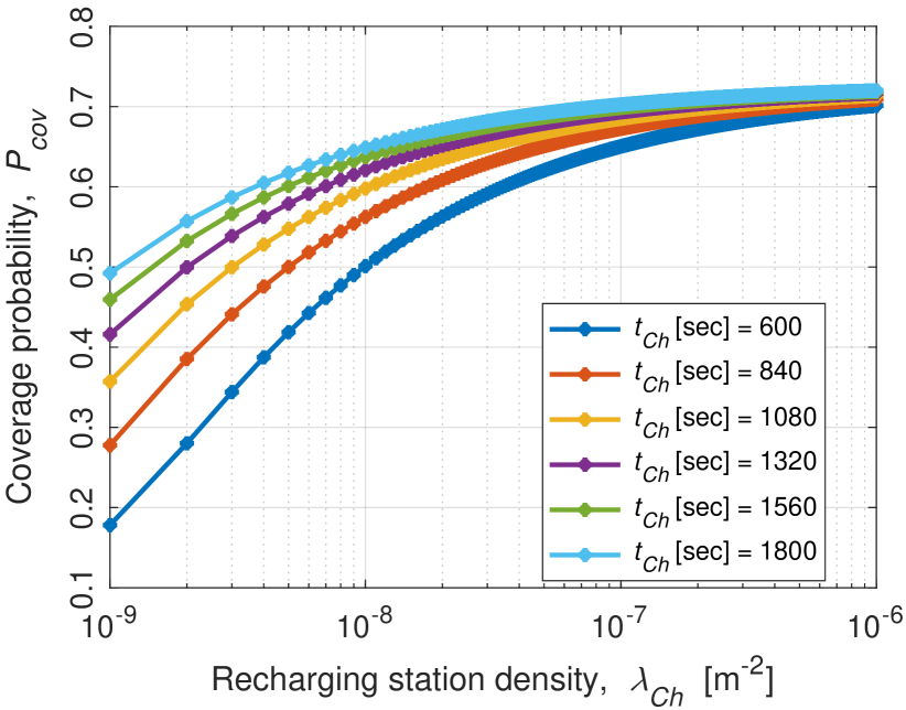
(a)

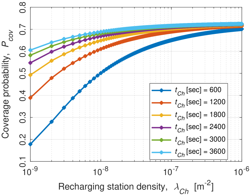
(b)

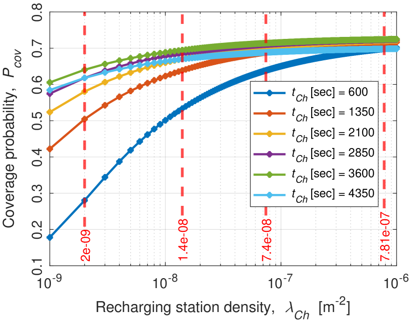
(c)

Figure 3: Coverage probability, $P_{cov}$, vs. recharging station density, $\lambda_{Ch}$, for different $t_{Ch}$: (a) half-charged; (b) fully-charged; (c) overflowed.

We first investigate the effect of varying recharging time on the coverage probability for an increasing recharging station density. For this analysis, using (3) for the considered $B_{\textrm{max}}$ and $\xi_{Ch}$ values, we know that $t_{Ch}^{sat}$ should be $3600$ seconds, i.e., $1$ hour, which is typical for commercial UAVs. Fig. 3(a) depicts what happens when the UAV stays at the recharging station until its battery gets half-full gradually. Here, we observe that, depending on the recharging level, certain discrepancies arise, which are especially evident for lower densities of recharging stations. For example, in the case of $0.001$ stations per km², $P_{cov}$ gets $2.7$ times better when $t_{Ch}$ is increased from $600$ to $1800$ seconds. This effect is less apparent for higher $\lambda_{Ch}$ because finding a recharging station becomes more likely for the UAV; hence, it may not need to depend heavily on the charge in its battery due to the increased recharging possibility. Numerically speaking, $P_{cov}$ increases only up to $1.3$ times for the same increment in $t_{Ch}$ when $\lambda_{Ch}$ is ten times higher, i.e., $0.01$ per km². When we look at the fully charged case shown in Fig.3(b), which can be considered ideal in theory, we see that the performance gap increases for lower-density values. Unsurprisingly, a fully-charged battery can help the UAV achieve better coverage, especially at a low $\lambda_{Ch}$, compared to those of partially-charged cases. Finally, in Fig.3(c), we analyze the case when the battery overflowed, i.e., when the UAV continues to stay at the recharging station after its battery gets fully charged. From (1), we know that increasing $t_{Ch}$ beyond saturation is unsuggested since the service probability, $P_{e}$, and hence $P_{cov}$, is inversely proportional to it. However, Fig.3(c) reveals that this might not be the case always. As seen, when the battery is charged for $4350$ seconds ($>\!t_{Ch}^{sat}$), it is still possible to obtain higher $P_{cov}$ compared to the partial charge cases, depending on $\lambda_{Ch}$. For example, $t_{Ch}$ of $600$ seconds can only outperform the overflowed case when $\lambda_{Ch}$ is $7.81\times 10^{-6}$m^-2 or higher. Similar comments also hold for other $t_{Ch}$ values (except for $t_{Ch}^{sat}$), as can be seen from the dashed red lines perpendicular to the x-axis, where the $\lambda_{Ch}$ threshold significantly reduces for increasing charge level towards the full battery, e.g., $2\times 10^{-9}$m^-2 for $t_{Ch}$ of $2850$ seconds. The take-home message from this analysis is that a relatively empty battery might be worse than overstaying at the recharging station, e.g., for maintenance purposes, if the application mandates a certain level of $\lambda_{Ch}$.
Next, we extend our discussion to the impact of using batteries of different sizes on the coverage probability for varying charging times. As can be seen from Fig. 4(a), in the case of a partial charge, all batteries show the same performance until $t_{Ch}=1440$ seconds, i.e., when the battery of size $308$Wh gets full. That is because all batteries are charged to the same level at that $t_{Ch}$ value regardless of their total size, $B_{\textrm{max}}$. The same phenomenon is also observed for the remaining batteries until the one with the smallest size reaches its $t_{Ch}^{sat}$, where the respective $P_{cov}$ starts its dramatic decay due to overflow. Fig. 4(a) and Fig. 4(b) are for different densities of stations; $10^{-9}$ and $10^{-6}$ [m^-2], respectively. Although $t_{Ch}^{sat}$ of each battery remains the same, the achievable $P_{cov}$ changes dramatically due to the clockwise rotation of the behavior.

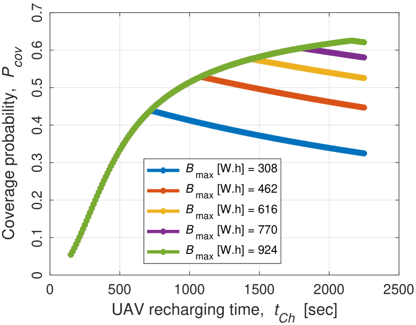
(a)

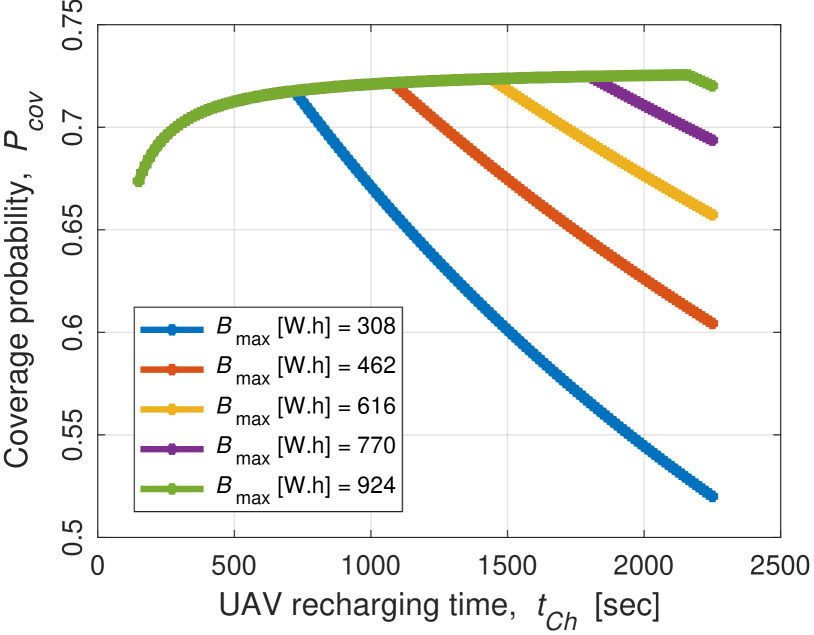
(b)

Figure 4: Coverage probability, $P_{cov}$, vs. recharging time, $t_{Ch}$, for different $B_{\textrm{max}}$: (a) @$\lambda_{Ch}\!=\!10^{-9}\!$ [m^-2]; (b) @$\lambda_{Ch}\!=\!10^{-6}\!$ [m^-2].

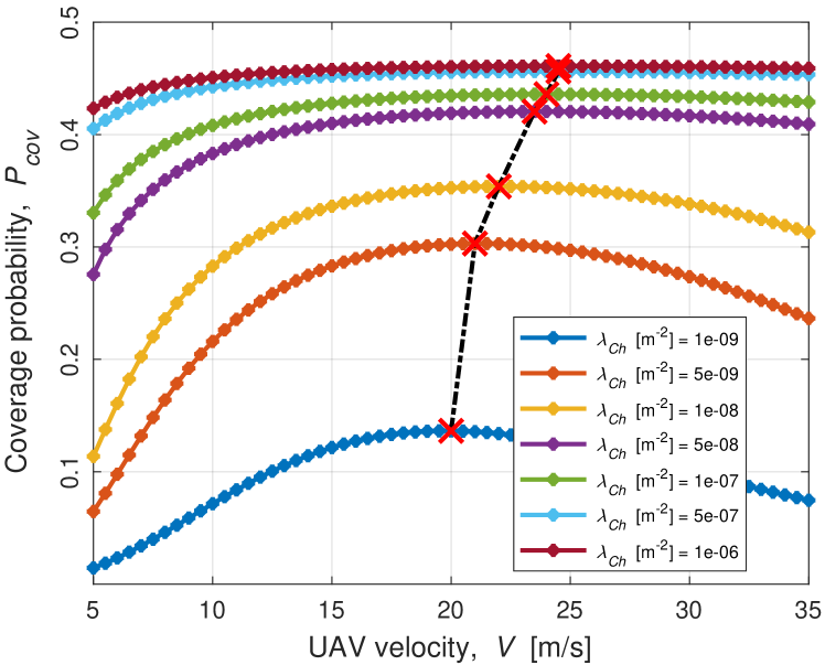
Figure 5: Coverage probability, $P_{cov}$, as a function of UAV velocity, $V$, for varying $\lambda_{Ch}$ values.

We lastly focus on understanding how the UAV velocity affects the coverage performance depending on the recharging station density. Before explaining the results, we should note that Fig. 5 is produced for a $B_{\textrm{max}}$ of $192.5$Wh, i.e., the quarter of what Table I mentions, which is only charged until its half at the same rate. As seen, the impact of $V$ is negligible for high $\lambda_{Ch}$ due to the same reason explained earlier in this section. For low $\lambda_{Ch}$, on the other hand, the UAV should speed up to reach the nearest station faster, although that means an increased $P_{J}$. Due to the $P_{J}$ component, however, the increment in $V$ is only beneficial until a certain point, as shown with the black dashed line marking the optimal velocity values for each $\lambda_{Ch}$. Using a bigger battery and charging it to the ideal level, i.e., $100\%$ -no overflow, will diminish this behavior, forcing higher speeds only for low $\lambda_{Ch}$ values.

The results above suggest that for a given performance target, e.g., maximum $P_{cov}$ with minimum $\lambda_{Ch}$, shorter $t_{Ch}$, or a fixed $B_{\textrm{max}}$, the relevant design parameters can be tweaked as required. Considering that most of these parameters affect each other, e.g., the EIRP limit on $P_{T}$ alters not only $P_{\mathrm{LoS}}$ (due to the dictated $\theta_{B}$) but also the size of the event area and hence the number of sensors that can be powered (not within the scope of this study) and even their reporting frequencies, the network requires a holistic design approach as optimizing the trade-offs for the best performance achievable. We believe this paper provides a practice-based showcase on this, providing guidance for future efforts.

V Conclusions

This study investigates the factors affecting the coverage performance of sensors energized by UAVs with directional antennae, constituting an energy-neutral IoT network together with the multi-source EH recharging stations replenishing UAVs batteries. With this goal, We first derived the service probability as a function of UAV power consumption/velocity and battery size, recharging time and station density, and WPT duration. That was then joined with distance-conditioned coverage probability, incorporating the effects of directivity, the LoS/NLoS connectivity, and the non-linear EH model. The analyses revealed the design considerations for the best coverage with regard to FCC regulations, realistic rectenna and UAV operation, and minimum power requirements of sensors. Future works will focus on calculating the number of sensors that can be powered by UAVs. We will also try maximizing the communication throughput of sensors in the envisioned setting by optimizing the parameters/trade-offs that have been discussed in this study.

VI Acknowledgement

This work has been supported by the PETRAS National Centre of Excellence for IoT Systems Cybersecurity, funded by the UK EPSRC under grant number EP/S035362/1.

References

- [1] A. Baltaci et al., “A Survey of Wireless Networks for Future Aerial Communications (FACOM),” IEEE Communications Surveys & Tutorials, vol. 23, no. 4, pp. 2833–2884, 2021.
- [2] O. Cetinkaya and G. V. Merrett, “Efficient Deployment of UAV-powered Sensors for Optimal Coverage and Connectivity,” in IEEE Wireless Communications and Networking Conference (WCNC), 2020, pp. 1–6.
- [3] X. Yuan et al., “Joint Design of UAV Trajectory and Directional Antenna Orientation in UAV-enabled Wireless Power Transfer Networks,” IEEE Journal on Selected Areas in Communications, vol. 39, no. 10, pp. 3081–3096, 2021.
- [4] T. Long et al., “Energy Neutral Internet of Drones,” IEEE Communications Magazine, vol. 56, no. 1, pp. 22–28, 2018.
- [5] O. B. Akan et al., “Internet of Hybrid Energy Harvesting Things,” IEEE Internet of Things Journal, vol. 5, no. 2, pp. 736–746, 2018.
- [6] M. Alzenad et al., “3-D Placement of an Unmanned Aerial Vehicle Base Station (UAV-BS) for Energy-efficient Maximal Coverage,” IEEE Wireless Communications Letters, vol. 6, no. 4, pp. 434–437, 2017.
- [7] L. Xie et al., “UAV-enabled Wireless Power Transfer: A Tutorial Overview,” IEEE Transactions on Green Communications and Networking, vol. 5, no. 4, pp. 2042–2064, 2021.
- [8] H.-T. Ye et al., “Optimization for Wireless-powered IoT Networks enabled by an Energy-limited UAV Under Practical Energy Consumption Model,” IEEE Wireless Communications Letters, vol. 10, no. 3, pp. 567–571, 2020.
- [9] Y. Qin et al., “Performance Evaluation of UAV-enabled Cellular Networks with Battery-limited Drones,” IEEE Communications Letters, vol. 24, no. 12, pp. 2664–2668, 2020.
- [10] L. Zhang et al., “Energy-Efficient Trajectory Optimization for UAV-Assisted IoT Networks,” IEEE Transactions on Mobile Computing, vol. 21, no. 12, pp. 4323–4337, 2022.
- [11] V. Hassija et al., “A Distributed Framework for Energy Trading Between UAVs and Charging Stations for Critical Applications,” IEEE Transactions on Vehicular Technology, vol. 69, no. 5, pp. 5391–5402, 2020.
- [12] N. H. Chu et al., “Joint Speed Control and Energy Replenishment Optimization for UAV-assisted IoT Data Collection with Deep Reinforcement Transfer Learning,” IEEE Internet of Things Journal, pp. 1–1, 2022.
- [13] Z. Wei et al., “UAV-assisted Data Collection for Internet of Things: A Survey,” IEEE Internet of Things Journal, vol. 9, no. 17, pp. 15 460–15 483, 2022.
- [14] C. A. Balanis, Antenna Theory: Analysis and Design. John wiley & sons, 2015.
- [15] “Federal Communications Commission CFR, Title 47, Volume 1, Part 15,” https://www.govinfo.gov/app/details/CFR-2010-title47-vol1, 2010.
- [16] O. Cetinkaya and O. B. Akan, “Electric-Field Energy Harvesting From Lighting Elements for Battery-Less Internet of Things,” IEEE Access, vol. 5, pp. 7423–7434, 2017.
- [17] Y. Zeng et al., “Energy Minimization for Wireless Communication with Rotary-wing UAV,” IEEE Transactions on Wireless Communications, vol. 18, no. 4, pp. 2329–2345, 2019.
- [18] M. Wagih et al., “High-efficiency sub-1 GHz Flexible Compact Rectenna based on Parametric Antenna-rectifier Co-design,” in 2020 IEEE/MTT-S International Microwave Symposium (IMS), 2020, pp. 1066–1069.
- [19] P. N. Alevizos et al., “Nonlinear Energy Harvesting Models in Wireless Information and Power Transfer,” in 2018 IEEE 19th International Workshop on Signal Processing Advances in Wireless Communications (SPAWC). IEEE, 2018, pp. 1–5.
- [20] J. Li et al., “Joint Optimization on Trajectory, Altitude, Velocity, and Link Scheduling for Minimum Mission Time in UAV-aided Data Collection,” IEEE Internet of Things Journal, vol. 7, no. 2, pp. 1464–1475, 2019.
- [21] Z. Liao et al., “HOTSPOT: A UAV-assisted Dynamic Mobility-aware Offloading for Mobile-edge Computing in 3-D Space,” IEEE Internet of Things Journal, vol. 8, no. 13, pp. 10 940–10 952, 2021.
- [22] A. Almarhabi et al., “LoRa and High-altitude Platforms: Path Loss, Link Budget and Optimum Altitude,” in 2020 8th International Conference on Intelligent and Advanced Systems (ICIAS). IEEE, 2021, pp. 1–6.