Thermoelectric transport across a tunnel contact between two charge Kondo circuits

Abstract

Following a theoretical proposal on multi-impurity charge Kondo circuits [T. K. T Nguyen and M. N. Kiselev, Phys. Rev. B 97, 085403 (2018)] and the experimental breakthrough in fabrication of the two-site Kondo simulator [W. Pouse et al, Nat. Phys. (2023)] we investigate a thermoelectric transport through a double-dot charge Kondo quantum nano-device in the strong coupling operational regime. We focus on the fingerprints of the non-Fermi liquid and its manifestation in the charge and heat quantum transport. We construct a full-fledged quantitative theory describing crossovers between different regimes of the multi-channel charge Kondo quantum circuits and discuss possible experimental realizations of the theory.

I Introduction

Thermoelectric materials have been investigated in recent years thanks to their ability to generate electricity from waste heat or being used as solid-state Peltier coolers TE_materials . The mechanism of converting of heat into voltage known as the Seebeck effect Seebeck is associated with the emergence of the electrostatic potential across the hot and cold ends of the thermocouple Seebeck1 ; Seebeck2 while no electric current flows through the system. The Peltier effect is manifested by the creation of the temperature difference between the junctions when the electric current flows through the thermocouple.

After theoretical predictions have been suggested that the thermoelectric efficiency could be greatly enhanced through nano-structural engineering in the mid-1990s, many complex nano-structured materials were studied in both theory and experiment lowD_TE_materials ; lowD_TE_materials1 ; Blanter ; Kisbook . Nano-electric circuits based on one or a few quantum dots (QDs), which are highly controllable and fine-tunable, can provide important information about the effects of strong electron-electron interactions, interference effects and resonance scattering on the quantum charge, spin and heat transport.

One of the fundamental motivations of the thermoelectric studies is to enhance thermoelectric power (absolute value of the Seebeck coefficient, TP). It is a challenge for both experimental fabrication of devices and theoretical suggestions for efficient mechanisms of heat transfer. In fact, the theoretical investigations showed that the TP of a single electron transistor (SET) was greatly enhanced in comparison with those of bulk materials staring_93 ; Turek_Matveev . Furthermore, the charge Kondo effect flensberg ; matveev ; furusakimatveev ; LeHur1 ; LeHur2 dealing with the degeneracy of the charge states of the QD (which is similar to the conventional Kondo effect Kondo ; Hewson ; TW1983 ; AFL1983 ; Kondo_review but does not require the system to have magnetic degree of freedom) can be a tool for intensification of the TP of a SET andreevmatveev ; TP_Kondo_exp . The building block of a charge Kondo circuit (CKC) is a large metallic QD strongly coupled to one (or several) lead(s) through an (or several) almost transparent single-mode quantum point contact(s) [QPC(s)]. In the orthodoxal charge Kondo theory flensberg ; matveev ; furusakimatveev , the electron location (namely, in or out of QD) is treated as an iso-spin variable, while two spin projections of electrons are associated with two (degenerate, in the absence of external magnetic field) conduction channels in the conventional Kondo problem. External magnetic field lifts out the channel degeneracy resulting in a crossover from two channel Kondo (2CK) regime at the vanishing magnetic field to the single channel Kondo (1CK) regime at the strong external field thanh2010 . As a result, the behavior of the system continuously changes from non-Fermi liquid (NFL) to the Fermi liquid (FL) states respectively. The interplay between NFL-2CK and FL-1CK regimes in thermoelectric transport through the SET has been investigated LeHur2 ; thanh2010 ; thanh2015 ; thanh2018 ; Anton2022 ; Thanh_VN_2 ; Thanh_VN_3 ; Kis2023 . The charge transport in 1CK and 2CK regimes were studied extensively numerically in Refs.Num1 ; Num2 ; Num3 ; Num4 . The effects of the electron-electron interactions in the charge Kondo simulators have been considered recentlyAnton2022 ; Thanh_VN_3 ; Thanh_VN_1 ; thanh2023 .

Recently, CKCs operated in the integer quantum Hall (IQH) regime have been implemented in breakthrough experiments pierre2 ; pierre3 . With the advantage that the number of Kondo channels is determined by the number of QPCs attached to the metallic QD, these experiments have opened an access to investigation of the multi-channel Kondo (MCK) problem experimentally. The dominant characteristic of a specific MCK setup is a NFL picture NB1980 ; Cox1998 ; AL1993 which is associated with $Z_{M}$ symmetry. For instance, the NFL-2CK AD1984 ; FGN_1 ; FGN_2 is explained by Majorana fermions gogolin ; Toulous_limit , the NFL-3CK physics is related to $Z_{3}$ parafermions Z3_1 ; Z3_2 ; Z3_3 ; Z3_4 ; Z3_5 ; Z3_6 . Therefore, switching between $Z_{2k+1}$ and $Z_{2k}$ low temperature fixed points by controlling the reflection amplitudes of the QPCs, can provide a route to investigate the crossovers between states with different parafermion fractionalized zero modes thanhprl .

As a CKC is considered as an artificial quantum simulator for the technology of quantum computer, scaling up the CKCs to clusters or lattices is challenging and it is important to understand the nature of the coupling between neighboring QDs. For this motivation, the experiment Gordon2023 has implemented a two-island charge Kondo device in which two QDs are coupled together and each one is also strongly coupled to an electrode through a QPC. The authors investigated the quantum phase transition at the triple point where the charge configurations are degenerate. Being more than the two-impurity Kondo (2IK) model, the two-site charge Kondo circuit is relevant to the Kondo lattice systems. Furthermore, the deeper theoretical investigation of the strong central coupling of this setup Karki2022 ; Z3_DCK in the Toulouse limit showed that a $Z_{3}$ parafermion emerging at the critical point, was already present in the experimental device of Ref. Gordon2023 .

In this work, we revisit the model proposed in Ref. thanh2018 which contains a tunnel contact between two CKCs where each one is set up in either FL or NFL state (see Fig. 1) with a two-fold goal. First, we examine the behavior of TP in order to find a mechanism to enhance it. Secondly, we show the existence of Majorana fermions in this double charge Kondo circuit (DCKC). The nonperturbative solution is obtained which allows to monitor and control all FL-NFL crossovers. The new energy scale associated with the inverse lifetime of the emergent Majorana fermions controls four different regimes of thermoelectric transport based on the window of parameters. Moreover, the non-perturbative results reported in this paper complete a full-fledged theory of the non-Fermi liquid to Fermi liquid crossover in the DCKC.

The paper is organized as follows. We describe the proposed experimental setup and the theoretical model in Sec. II. General equations for the thermoelectric coefficients are presented and the nonperturbative solution is discussed in Sec. III. The Sec. IV represents the correlation function in different cases. The main results are discussed in Sec. V. We conclude our work in Sec. VI.

II Proposed experimental setup and theoretical model

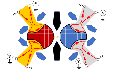
Figure 1: Schematic of a weak link between two charge Kondo circuits (CKC). Each circuit consists of a large metallic island (QD), which is embedded into two-dimensional electron gas (2DEG) and connects to two large electrodes through the single-mode quantum point contacts (QPCs). The 2DEG (plain area) is in the integer quantum Hall regime $\nu=1$. The red line with arrows denotes the chiral edge mode which backscatters at the center of the narrow constriction. The QPCs are fine tuned by field effects in split gates (blue boxes) to different regimes. We name the QPCs in the left CKC as $\text{QPC}_{11}$, $\text{QPC}_{12}$ and the QPCs in the right CKC as $\text{QPC}_{21}$, $\text{QPC}_{22}$. The right CKC (grey color) is at the reference temperature $T$ while the left circuit (orange color) is at higher temperature $T+\Delta T$.

We consider a DCKC device (see Fig. 1) formed by two CKCs describing a very recent experiment Gordon2023 . The building block for each CKC is a QD-QPC structure implemented in experiment pierre2 . The QD is a large metallic island (the dark-red and blue cross-hatched areas surrounded by the black lines) electronically connected to a two-dimensional electron gas (2DEG, the orange and grey continuous areas). The 2DEG is connected to two large electrodes through two QPCs. Applying a strong magnetic field perpendicular to the 2DEG plane can control the 2DEG in the IQH regime at the filling factor $\nu=1$. The QPCs are fine-tuned (by field effects in the split gates illustrated by the blue boxes) to the high transparency regime corresponding to weak backscattering of the chiral edge mode (red solid lines with arrows). We investigate the regime of equal reflection amplitudes at two QPCs in each CKC: $|r_{11}|=|r_{12}|=|r_{1}|$ and $|r_{21}|=|r_{22}|=|r_{2}|$. Therefore, each CKC is a 2CK setup. Indeed, the CKC can be tuned into a 1CK model by simply deactivating one of the two QPCs in it. These two CKCs are connected together by a weak tunneling (barrier, weak link) between two QDs. In order to study the thermoelectric transport through the DCKC system, the left CKC is set up at higher temperature $T+\Delta T$ in comparison with the right circuit, which is at temperature $T$. The temperature drops at the central weak link.

The spinless Hamiltonian describing the two CKCs coupled weakly at the center in which each QD is coupled strongly to the lead through two QPCs (Fig. 1) has the form $H$$=$$H_{L}+H_{T}+H_{R}$, where

$$H_{T}=(td_{1}^{\dagger}d_{2}+\text{h.c.}).$$ (1)

describes the tunneling between two dots, $d_{j}$ stands for the electrons in the dot $j,$ $j=1,2$. The Hamiltonian $H_{L/R}$ describing each (QD-QPC) structure has the form $H_{L/R}$$=$$H_{0L/R}+H_{CL/R}+H_{sL/R}$. The Hamiltonian $H_{0,j}$ ($j=L,R$) describing the propagation of the edge states is given by

$$H_{0,j} = -iv_{F}\sum_{\alpha=1,2}\!\!\!\!\int_{-\infty}^{\infty}\!\!\!\!dx\left[\psi_{R,j,\alpha}^{\dagger}(x)\partial_{x}\psi_{R,j,\alpha}(x)\right.$$ (2)

$$\left.-\psi_{L,j,\alpha}^{\dagger}(x)\partial_{x}\psi_{L,j,\alpha}(x)\right],$$

where $\psi_{L/R,\alpha,j}$ represents the incoming/outgoing chiral fermions at the QPC $\alpha$ of the CKC $j$, and $v_{F}$ is the Fermi velocity. For simplicity we assume that the Fermi velocity is the same for all QPCs. Note that the operator $d_{j}$ can be expressed through the fermionic operators $\psi_{j,\alpha}$ as $d_{j}=\sum_{\alpha=1,2}\psi_{j,\alpha}(-\infty)$. The Hamiltonian $H_{C,j}$ characterizes the Coulomb interaction in the dot andreevmatveev ; Aleiner98

$$H_{C,j}\!=E_{C,j}\!\int_{0}^{\infty}\!\!\!\!dx\left[n_{j}-\!\!\sum_{\alpha=1,2}\!\psi_{j,\alpha}^{\dagger}(x)\psi_{j,\alpha}(x)-N_{j}\right]^{2}\!,$$ (3)

where $E_{C,j}$ is the charging energy of the QD $j$. The number of electrons entering the dot (taking values $0,1$ in units of $e$) through the weak link and the QPCs is demonstrated by the operator $n_{j}$ and the second term in the parentheses (with $\psi_{j,\alpha}=\psi_{L,j,\alpha}+\psi_{R,j,\alpha}$) respectively. $N_{j}$ is the normalized gate voltage, controlled by plunger gates (not shown in Fig. 1). The Hamiltonian $H_{s,j}$ describing the backward scattering at the QPCs, with the reflection amplitude $r_{j,\alpha}$, writes

$$\!\!H_{s,j}\! =-\frac{D}{\pi}\sum_{\alpha=1,2}\!\!|r_{j,\alpha}|\left[\psi_{R,j,\alpha}^{\dagger}\left(0\right)\psi_{L,j,\alpha}\left(0\right)+h.c.\right],$$ (4)

$D$ is a bandwidth.

The appropriate technique to describe the interacting electrons in the QD and QPCs is the bosonized representation gogolin ; giamarchi . The detailed bosonization of the Hamiltonian $H$ can be read in Refs. andreevmatveev ; thanh2018 . One should notice that the fermionic fields are related to the bosonic field at the QPC $\alpha$ of the CKC $j$ as $\psi_{L/R,j,\alpha}(x)\sim e^{-i\phi_{j,\alpha}(x)}$. The actions in the bosonic language are presented in the Section IV.

III General formulas for current, electric conductance and thermoelectric coefficient

In order to study the thermoelectric effects in the DCKC with a small temperature drop $\Delta T\ll T$ at the weak link between two QDs, we consider the tunnel charge current across the tunnel contact in the tunneling amplitude $|t|$ as

$$I=-2\pi e|t|^{2}\!\!\!\int_{-\infty}^{\infty}\!\!\!\!\!\!d\epsilon\>\nu_{1}(\epsilon)\nu_{2}(\epsilon)\left[f_{1}(\epsilon)-f_{2}(\epsilon)\right]~{}.$$ (5)

Here we denote the Fermi distribution functions as $f_{1}(\epsilon)=f(\epsilon,T+\Delta T)$, $f_{2}(\epsilon)=f(\epsilon+e\Delta V,T)$, with $\Delta V$ is an applied thermo-voltage to implement a zero-current condition for the electric current between the source and drain, and we define the densities of states $\nu_{j}(\epsilon)=-\left(1/\pi\right)\cosh\left(\frac{\epsilon}{2T}\right)\int_{-\infty}^{\infty}{\cal G}_{j}\left({\displaystyle\left(1/2T\right)+it}\right)e^{i\epsilon t}dt$ with $\mathcal{G}_{j}(\tau)=-\langle T_{\tau}\,d_{j}(\tau)d_{j}^{\dagger}(0)\rangle$ are exact Green’s Functions (GF) in the terminals $j=1,2$. The thermoelectric coefficients in the linear response regime are computed as follows. The electric conductance casts a form

$$\!\!\!G=\left.\frac{\partial I}{\partial\Delta V}\right|_{\Delta T=0}\!\!\!=\frac{e^{2}|t|^{2}}{2\pi T}\int_{-\infty}^{\infty}\!\!\!d\epsilon\int_{-\infty}^{\infty}\!\!\!dt_{1}$$

$$\!\!\!\!\!\!\times{\cal G}_{1}\left({\displaystyle\frac{1}{2T}+it_{1}}\right)e^{i\epsilon t_{1}}\!\!\!\int_{-\infty}^{\infty}\!\!\!dt_{2}{\cal G}_{2}\left({\displaystyle\frac{1}{2T}+it_{2}}\right)e^{i\epsilon t_{2}},$$ (6)

and the thermoelectric coefficient is given by

$$\!\!\!\!\!\!G_{T}=\left.\frac{\partial I}{\partial\Delta T}\right|_{\Delta V=0}\!\!\!\!=-\frac{e|t|^{2}}{2\pi T^{2}}\int_{-\infty}^{\infty}d\epsilon\,\epsilon\!\!\!\int_{-\infty}^{\infty}\!\!\!\!dt_{1}$$

$$\!\!\!\!\!\!{\cal G}_{1}\left({\displaystyle\frac{1}{2T}+it_{1}}\right)e^{i\epsilon t_{1}}\!\!\!\!\int_{-\infty}^{\infty}\!\!\!\!dt_{2}{\cal G}_{2}\left({\displaystyle\frac{1}{2T}+it_{2}}\right)e^{i\epsilon t_{2}}.$$ (7)

The thermopower (or the Seebeck coefficient) in the linear regime is defined at $I=0$ as

$$S=-\left.\frac{\Delta V}{\Delta T}\right|_{I=0}=\frac{G_{T}}{G}.$$ (8)

Following Matveev and Andreev andreevmatveev we define $d_{j}(\tau)=\psi_{j,\alpha}^{(0)}(\tau)F_{j}(\tau)$, where $\psi_{j,\alpha}^{(0)}(\tau)=\psi_{\alpha,j}^{(0)}(-\infty,\tau)$, the operator $F_{j}$ obeys the commutation relation $\left[F_{j},n_{j}\right]=F_{j}$ and takes into account effects of interaction and reflection given by Eqs. (3,4). Since the operators $\psi_{j,\alpha}^{(0)}$ and $F_{j}$ are decoupled, the GFs at imaginary times are factorized as ${\cal G}_{j}(\tau_{j})=-\left(\nu_{0j}\pi T/\sin\left[\pi T\tau_{j}\right]\right)K_{j}(\tau_{j})$, where $\nu_{0j}$ is the density of states in the dot $j$ without interaction and $K_{j}(\tau)=\langle T_{\tau}F_{j}(\tau)F_{j}^{\dagger}(0)\rangle$ accounts for interaction effects. As a result, the electric conductance and the thermoelectric coefficient are given by:

$$\!\!\!G=\frac{\pi}{2}G_{C}T\!\!\int_{-\infty}^{\infty}\!\!\!\frac{dt}{\cosh^{2}(\pi Tt)}{\displaystyle K_{1}\!\left(\frac{1}{2T}+it\right)\!K_{2}\!\left(\frac{1}{2T}-it\right),}\;\;\;$$ (9)

$$\!\!\!\!\!\!\!G_{T} = -\frac{i\pi G_{C}}{4e}\int_{-\infty}^{\infty}\frac{dt}{\cosh^{2}(\pi Tt)}$$ (10)

$$\times\left[\left(\partial_{t}K_{1}\left(\frac{1}{2T}+it\right)\right)K_{2}\left(\frac{1}{2T}-it\right)\right.$$

$$-\left.K_{1}\left(\frac{1}{2T}+it\right)\left(\partial_{t}K_{2}\left(\frac{1}{2T}-it\right)\right)\right],$$

where $G_{C}=2\pi e^{2}\nu_{01}\nu_{02}|t|^{2}$ is a conductance of the central (tunnel) area. The computation of thermoelectric coefficients in Eqs. (9-10) misprint requires the explicit form of the correlation functions $K_{1,2}\left(\frac{1}{2T}\pm it\right)$.

IV Correlation function $K_{j}(\tau)$:

The time-ordered correlation function $K_{j}(\tau)$ is defined through the operator $F_{j}$. The process where the number of electron entering the $\text{QD}_{j}$ through the weak link is increased from $0$ to $1$ at time $t=0$ and decreased back to $0$ at time $t=\tau$ is demonstrated by $F_{j}(\tau)F_{j}^{\dagger}(0)$. Therefore, the operator $n_{j}$ is replaced by $n_{j\tau}\left(t\right)=\theta\left(t\right)\theta\left(\tau-t\right)$ with $\theta\left(t\right)$ is the unit step function, and the correlation function $K_{j}(\tau)$ is computed through the functional integration over the bosonic fields $K_{j}(\tau)=Z_{j}(\tau)/Z_{j}(0)$.

IV.1 The 1CK case: Perturbative solution:

In the case one CKC is settled down in the FL-1CK state by decoupling one of the two QPCs, the functional integral writes

$$\!\!\!\!\!\!\!\!Z_{j}(\tau)\! = \!\!\int\!\mathcal{D}\phi_{j}\exp\left[-\mathcal{S}_{0,j}-\mathcal{S}_{C,j}(\tau)-\mathcal{S}_{s,j}\right],$$ (11)

where $\mathcal{S}_{0,j}$, $\mathcal{S}_{C,j}$, and $\mathcal{S}_{s,j}$ are Euclidean actions describing the free (non-interacting) one-dimensional Fermi gas, Coulomb blockade in the QD and the backscattering at the QPC of the CKC $j$, respectively. They are written as

$$\!\!\!\!\mathcal{S}_{0,j}\!\! = \!\frac{v_{F}}{2\pi}\int_{0}^{\beta}\!\!\!\!dt\!\!\int\!\!dx\!\left[\frac{(\partial_{t}\phi_{j})^{2}}{v_{F}^{2}}+(\partial_{x}\phi_{j})^{2}\right],$$ (12)

$$\!\!\!\!\mathcal{S}_{C,j}\!\! = \!E_{C,j}\!\int_{0}^{\beta}\!\!\!\!dt\left[n_{j\tau}(t)+\frac{1}{\pi}\phi_{j}(0,t)-N_{j}\right]^{2}\!,$$ (13)

$$\mathcal{S}_{s,j}\!\! = \!\!-\frac{2D}{\pi}|r_{j}|\!\int_{0}^{\beta}\!\!\!dt\cos\left[2\phi_{j}(0,t)\right].$$ (14)

with $\beta=1/T$. One should notice that the bosonic field describing the electrons moving through the constriction is blocked by the Coulomb interaction in the QD. Therefore, $Z_{j}(\tau)$ can be computed perturbatively over $|r_{j}|$ for the small backscattering at the QPC ($|r_{j}|\ll 1$), and the correlation function $K_{j}(\tau)$ then is

$$K_{j}\!\left(\tau\right) = \!\left(\frac{\pi^{2}T}{\gamma E_{C,j}}\right)^{2}\!\!\!\frac{1}{\sin^{2}\left(\pi T\tau\right)}\left[1-2\gamma\xi|r_{j}|\cos\left(2\pi N_{j}\right)\right.$$ (15)

$$\left.+4\pi^{2}\xi\gamma|r_{j}|\frac{T}{E_{C,j}}\sin\left(2\pi N_{j}\right)\cot\left(\pi T\tau\right)\right]~{},$$

with $\gamma=e^{C}$, $C\approx 0.577$ is Euler’s constant, $\xi=1.59$ is a numerical constant andreevmatveev .

IV.2 The symmetric 2CK case: Nonperturbative solution:

For convenient calculation later, one can define the variables $\phi_{j,\rho/\sigma}=\phi_{j,1}\pm\phi_{j,2}$ so-called charge/spin fields. The functional integral in this case is written as:

$$\!\!\!\!\!\!\!\!Z_{j}(\tau)\! = \!\!\!\!\!\prod_{\lambda=\rho,\sigma}\!\int\!\mathcal{D}\phi_{j\lambda}\exp\left[-\mathcal{S}_{0,j}-\mathcal{S}_{C,j}(\tau)-\mathcal{S}_{s,j}\right],$$ (16)

where $\mathcal{S}_{0,j}$, $\mathcal{S}_{C,j}$, and $\mathcal{S}_{s,j}$ are Euclidean actions describing the free Fermi liquid, Coulomb blockade in the QD and the backscattering at the QPCs of the CKC $j$ , respectively. The action $\mathcal{S}_{0,j}$ is presented as a sum of two independent actions

$$\!\!\!\!\mathcal{S}_{0,j}\!\! = \!\!\!\!\sum_{\lambda=\rho,\sigma}\!\frac{v_{F}}{2\pi}\int_{0}^{\beta}\!\!\!\!dt\!\!\int\!\!dx\!\left[\frac{(\partial_{t}\phi_{j,\lambda})^{2}}{v_{F}^{2}}+(\partial_{x}\phi_{j,\lambda})^{2}\right].$$ (17)

The Coulomb blockade action $\mathcal{S}_{C,j}$ in bosonic representation reads

$$\!\!\!\!\mathcal{S}_{C,j}\!\! = \!E_{C,j}\!\int_{0}^{\beta}\!\!\!\!dt\left[n_{j\tau}(t)+\frac{\sqrt{2}}{\pi}\phi_{j,\rho}(0,t)-N_{j}\right]^{2}\!.$$ (18)

The contribution $\mathcal{S}_{s,j}$ in the action of each CKC characterizes the weak backscattering at the QPCs is

$$\!\!\mathcal{S}_{s,j}\!\!=\!\!-\frac{2D}{\pi}|r_{j}|\!\int_{0}^{\beta}\!\!\!dt\cos\left[\sqrt{2}\phi_{j,\rho}(0,t)\right]\cos\left[\sqrt{2}\phi_{j,\sigma}(0,t)\right].\;\;\;\;$$ (19)

In the absence of backscattering $|r_{j}|=0$, the functional integral Eq.(16) is Gaussian. The correlator $K_{j}^{(0)}(\tau)\equiv K_{j}(\tau)|_{r=0}=K_{j,\rho}(\tau)$ is computed at low temperature $T\ll E_{C}$ and at $\tau\gg E_{C}^{-1}$:

$$K_{j,\rho}(\tau)=\frac{\pi^{2}T}{2\gamma E_{C,j}}\frac{1}{|\sin(\pi T\tau)|}.$$ (20)

The perturbative results (see Ref.andreevmatveev ) showed that the thermoelectric properties of the system are controlled by charge and spin fluctuations at low frequencies (below $E_{C,j}$). One should notice that the effect of small but finite $|r_{j}|$ on the charge modes is negligible in comparison with the Coulomb blockade but it changes the low frequency dynamics of the unblocked spin modes dramatically. The correlation function can be split into charge and spin components as $K_{j}(\tau)=K_{j\rho}(\tau)K_{j\sigma}(\tau)$, with $K_{j\sigma}(\tau)=Z_{j\sigma}(\tau)/Z_{j\sigma}(0)$. We simply replace the $\cos\left[\sqrt{2}\phi_{j,\rho}(0,t)\right]$ in action Eq. (19) by the $\langle\cos[\sqrt{2}\phi_{j,\rho}(0,t)]\rangle_{\tau}=\sqrt{2\gamma E_{C,j}/\pi D}\cos\left[\pi N_{j}-\chi_{j\tau}(t)\right]$, with $\chi_{j}(t)=\pi n_{j\tau}(t)+\delta\chi_{j\tau}(t)$ , $\delta\chi_{j\tau}(t)\approx\frac{\pi^{2}T}{2E_{C,j}}\left[\cot(\pi T(t-\tau)-\cot(\pi Tt)\right]$ and obtain the effective action for the spin degrees of freedom in the form

$$\!\!\!\!\mathcal{S}_{\tau j}\! = \!\!\int\!\!dx\int_{0}^{\beta}\!\!\!\!dt\frac{v_{F}}{2\pi}\left[\frac{(\partial_{t}\phi_{j,\sigma})^{2}}{v_{F}^{2}}+(\partial_{x}\phi_{j,\sigma})^{2}\right]$$ (21)

$$-\int_{0}^{\beta}dt\sqrt{\frac{4D}{v_{F}}}\tilde{\lambda}_{j\tau}(t)\cos\left[\sqrt{2}\phi_{j,\sigma}(0,t)\right],$$

where

$$\tilde{\lambda}_{j\tau}(t)=\Lambda_{j}(-1)^{n_{\tau}(t)}\cos\left[\pi N_{j}-\delta\chi_{j\tau}(t)\right],$$

$$\Lambda_{j}=|r_{j}|\sqrt{\frac{2\gamma v_{F}E_{C,j}}{\pi D}}.$$ (22)

After performing the refermionization, our model [as shown in Eq. (21)] is mapped onto an effective Anderson model, which is described by Hamiltonian

$$\!\!\!\!\!\!H_{j,\tau}^{eff}\!\left(t\right)\!=\!\!\int\!\left[v_{F}kc_{j,k}^{\dagger}c_{j,k}\!-\tilde{\lambda}_{j\tau}\!(t)(c+c^{\dagger})\!\left(c_{j,k}\!-c_{j,k}^{\dagger}\right)\!\right]\!dk,\;\;\;\;\;\;\;$$ (23)

in which the operators $c_{j,k}^{\dagger}$ and $c_{j,k}$ satisfying the anti-commutation relations$\left\{c_{j,k},c_{j,k^{{}^{\prime}}}^{\dagger}\right\}=\delta\left(k-k^{{}^{\prime}}\right)$ create and destroy chiral fermions; $c$ is a local fermionic annihilation operator anti-commuting with $c_{j,k}^{\dagger}$ and $c_{j,k}$. We see that the model is free and equivalent to a resonant level model where the leads are coupled to Majorana fermion $\eta=(c+c^{\dagger})/\sqrt{2}$ on the impurity. The time dependent Hamiltonian (23) can be split into $H_{j,0}^{eff}+H_{j,\tau}^{\prime}\left(t\right)$ by replacing $\tilde{\lambda}_{j\tau}(t)\rightarrow\tilde{\lambda}_{j\tau}(t)/\left(-1\right)^{n_{\tau}\left(t\right)}$. The time-independent Hamiltonian part $H_{j,0}^{eff}$ is $H_{j,\tau=0}^{eff}$ while the correction is

$$\!\!\!\!\!H_{j,\tau}^{\prime}\left(t\right)=2\Lambda_{j}\!\left\{\cos\left[\pi N_{j}\right]-\cos\left[\pi N_{j}\!-\delta\chi_{j\tau}(t)\right]\right\}\eta\zeta,$$ (24)

with $\zeta=\int_{-\infty}^{\infty}\left(c_{j,k}-c_{j,k}^{\dagger}\right)dk/\sqrt{2}$ describes the Majorana fermion of the leads in the resonant level model. Our solution, being nonperturbative in $|r_{j}|$ and accounting for low-frequency dynamics of the spin modes, leads to the appearance of the Kondo-resonance width $\Gamma_{j}$ in the vicinity of Coulomb peaks

$$\Gamma_{j}\left(N_{j}\right)=\frac{8\gamma E_{C,j}}{\pi^{2}}|r_{j}|^{2}\cos^{2}(\pi N_{j}).$$ (25)

We then compute the correlation function straightforwardly and obtain the zero-order term corresponding to the Hamiltonian part $H_{j,0}^{eff}$ as

$$K_{j}^{(0)}\!\left(\frac{1}{2T}+it\right)=\frac{\pi T\Gamma_{j}}{\gamma E_{C,j}}\frac{1}{\cosh(\pi Tt)}$$

$$\times\int_{-\infty}^{\infty}\frac{e^{\omega\left(1/2T+it\right)}}{\left(\omega^{2}+\Gamma_{j}^{2}\right)\left(1+e^{\omega/T}\right)}d\omega,$$ (26)

and the first-order term when the correction Hamiltonian part $H_{j,\tau}^{\prime}\left(t\right)$ is taken into account, is

$$K_{j}^{(1)}(\frac{1}{2T}+it)=\!-\frac{4T}{E_{C,j}}\frac{|r_{j}|^{2}\sin\left(2\pi N_{j}\right)}{\cosh(\pi Tt)}$$

$$\times\ln\left(\frac{E_{C,j}}{T+\Gamma_{j}}\right)\int_{-\infty}^{\infty}\!\!\!\!\!\!d\omega\frac{\omega e^{\omega\left(\nicefrac{{1}}{{2T}}+it\right)}}{\left(\omega^{2}+\Gamma_{j}^{2}\right)\left(1+e^{\nicefrac{{\omega}}{{T}}}\right)}~{}.$$ (27)

The formulas (26) and (27) will be used to calculate the thermoelectric coefficients in the next Section.

V Main results

The first work of the Authors thanh2018 considered the weak effects of the non-Fermi liquid behaviour in the thermoelectric transport. The approach used in thanh2018 is based on accounting for the perturbative corrections to the transport off-diagonal coefficients and is limited by the perturbation theory domain of validity (high-temperature regime). These calculations, being very useful for understanding the flow towards the non-Fermi liquid intermediate coupling fixed point, neither become valid at the low-temperature regime, nor shed a light on reduction of the symmetry due to the emergency of the Majorana (parafermionic) states. The main idea of this work is to develop a controllable and reliable approach for the quantitative description of the Fermi-to-non-Fermi liquid crossovers and interplay around the intermediate coupling fixed points. It therefore provides a complementary study of the model thanh2018 and completes the theory of thermoelectrics in DCKCs.

V.1 Weak coupling between single- and two-channel charge Kondo circuits

In this case, for instance, we consider the left CKC is in the FL-1CK state while the right CKC is in the NFL-2CK state. We apply the correlation functions $K_{1}\left(\frac{1}{2T}+it\right)$ and $K_{2}\left(\frac{1}{2T}-it\right)$ as shown in Eqs. (15) and (26-27), respectively. The electric conductance is obtained as

$$G=\frac{\pi^{2}G_{C}T^{3}}{96\gamma^{3}E_{C,1}^{2}E_{C,2}}F_{G}\left(\frac{\Gamma_{2}}{T}\right),$$ (28)

with $F_{G}$ is a dimensionless parameter demonstrating the competition between the Kondo resonance of the right CKC $\Gamma_{2}$ and the temperature $T$. It is computed as

$$F_{G}\left(p_{2}\right) =\!\int_{-\infty}^{\infty}\!\!\!du\,J\left(p_{2},u\right),$$

$$\,J\left(p_{2},u\right) =\frac{\left[u^{2}+\pi^{2}\right]\left[u^{2}+9\pi^{2}\right]}{\cosh^{2}\left(\frac{u}{2}\right)\left[u^{2}+p_{2}^{2}\right]}.$$ (29)

The thermoelectric coefficient is given by

$$G_{T}=-\frac{\pi^{5}\xi G_{C}T^{3}\Gamma_{2}}{72e\gamma^{2}E_{C,1}^{3}E_{C,2}}F_{G}\left(\frac{\Gamma_{2}}{T}\right)|r_{1}|\sin\left(2\pi N_{1}\right)$$

$$\!\!-\frac{\pi G_{C}T^{3}}{360e\gamma^{2}E_{C,1}^{2}E_{C,2}}F_{T}\!\left(\frac{\Gamma_{2}}{T}\right)\!\!\left[\frac{2\pi^{2}\xi\Gamma_{2}}{E_{C,1}}|r_{1}|\sin\left(2\pi N_{1}\right)\right.$$

$$\left.+|r_{2}|^{2}\ln\left(\frac{E_{C,2}}{T+\Gamma_{2}}\right)\sin\left(2\pi N_{2}\right)\right],$$ (30)

with

$$F_{T}\left(p_{2}\right) =\!\int_{-\infty}^{\infty}\!\!\!du\,u^{2}J\left(p_{2},u\right).$$ (31)

Following the discussion in Ref. thanh2018 , based on the perturbative solution, the Seebeck effect on a weak link between 1CK and 2CK is characterized by the competition between the Fermi and non-Fermi liquids (see Eq. (24) in the Ref. thanh2018 ). However, in this part, it is true for high temperature $T\gg\Gamma_{2}$. At very low temperature, $T\ll\Gamma_{2}$, the TP behaves only the FL.

V.1.1 $T\gg\Gamma_{2}$ limit: Fermi-liquid on the left and non Fermi-liquid on the right CKC:

At temperature $T\gg\Gamma_{2}$ the expression in Eq. (30) reproduces the perturbative result as represented in Eq. (23) of Ref.thanh2018 . The TP is thus similar to the formula (24) in Ref.thanh2018 :

$$S = -\frac{4\pi^{3}\xi\gamma}{3e}|r_{1}|\frac{T}{E_{C,1}}\sin\left(2\pi N_{1}\right)$$ (32)

$$-\frac{526\gamma}{\pi^{2}e}|r_{2}|^{2}\ln\left(\frac{E_{C,2}}{T}\right)\sin\left(2\pi N_{2}\right).$$

The crossover line separating the two contributions in the TP is defined as follows:

$$\frac{789}{2\pi\xi}\ln\left(\frac{E_{C,2}}{\widetilde{T}}\right)\frac{E_{C,1}}{\widetilde{T}}=\frac{|r_{1}|}{|r_{2}|^{2}}.$$ (33)

If $\Gamma_{2}\ll T\ll\widetilde{T}$, NFL-2CK behavior of the TP is predicted to be pronounced. In the opposite limit, $T\gg\widetilde{T}\gg\Gamma_{2}$, the FL-1CK regime with the weak NFL-2CK corrections is expected.

V.1.2 $T\ll\Gamma_{2}$ limit: fully Fermi-liquid regime:

At temperature $T\ll\Gamma_{2}$ the expression in Eq. (30) induces the linear temperature term in the square brackets. The TP thus behaves the FL characteristic as

$$S=-\frac{7682\pi^{3}\xi\gamma}{5523e}\left[|r_{1}|\frac{T}{E_{C,1}}\sin\left(2\pi N_{1}\right)\right.$$

$$\left.\!\!+\frac{1431}{3841\pi^{2}\xi}|r_{2}|^{2}\ln\!\left(\!\frac{E_{C,2}}{\Gamma_{2}}\!\right)\!\frac{T}{E_{C,2}}\sin\left(2\pi N_{2}\right)\right].$$ (34)

In summary, in the situation of the weak coupling between single- and two-channel charge Kondo circuits, there exist two energy scales $\Gamma_{2}$ ($\Gamma_{2}\leq(8\gamma/\pi^{2})E_{C,2}|r_{2}|^{2}$) and $\widetilde{T}$ of temperature in the regime $(0,E_{C,2})$ in which one finds more chances for the FL picture than the NFL one.

V.2 Weak coupling between two two-channel charge Kondo circuits

We take into account both $K_{j}^{(0)}\left(\frac{1}{2T}+it\right)$, we have

$$G=\frac{G_{C}T^{2}}{24\gamma^{2}E_{C,1}E_{C,2}}F_{C}\left(\frac{\Gamma_{1}}{T},\frac{\Gamma_{2}}{T}\right),$$ (35)

with

$$F_{C}\left(p_{1},p_{2}\right)=\int_{-\infty}^{\infty}dz\int_{-\infty}^{\infty}du\,F\left(p_{1},p_{2},z,u\right),$$ (36)

$$F\left(p_{1},p_{2},z,u\right)=\frac{p_{1}p_{2}u\left[u^{2}+4\pi^{2}\right]}{\sinh\left(\frac{u}{2}\right)\left[\cosh\left(z\right)+\cosh\left(\frac{u}{2}\right)\right]}$$

$$\times\frac{1}{\left[\left(z+\frac{u}{2}\right)^{2}+p_{1}^{2}\right]\left[\left(z-\frac{u}{2}\right)^{2}+p_{2}^{2}\right]}.$$ (37)

The integral in Eq. (10) gives the zero value when we apply $K_{1,2}^{(0)}\left(\frac{1}{2T}\pm it\right)$ for both sides: $G_{T}^{(0)}=0$. We therefore need to consider the first order of the correlation function. We take into account, for instance, $K_{1}^{(0)}\left(\frac{1}{2T}+it\right)K_{2}^{(1)}\left(\frac{1}{2T}-it\right)$ and $K_{1}^{(1)}\left(\frac{1}{2T}+it\right)K_{2}^{(0)}\left(\frac{1}{2T}-it\right)$, we obtain the lowest order (we consider the model in the vicinity of the intermediate coupling fixed point) non-zero contribution to thermoelectric coefficient as follows

$$\!\!\!\!G_{T}^{(1)}=-\frac{G_{C}T^{3}}{24e\gamma\pi E_{C,1}E_{C,2}}$$

$$\!\!\!\!\!\!\!\!\times\left\{\frac{|r_{1}|^{2}}{\Gamma_{1}}\ln\left(\frac{E_{C,1}}{T+\Gamma_{1}}\right)\sin\left(2\pi N_{1}\right)F_{T,s}\left(\frac{\Gamma_{1}}{T},\frac{\Gamma_{2}}{T}\right)\right.$$

$$\!\!\!\!\!\!\!\!\!\!\!+\left.\frac{|r_{2}|^{2}}{\Gamma_{2}}\ln\left(\frac{E_{C,2}}{T+\Gamma_{2}}\right)\sin\left(2\pi N_{2}\right)F_{T,m}\left(\frac{\Gamma_{1}}{T},\frac{\Gamma_{2}}{T}\right)\right\},$$ (38)

where

$$\!\!\!\!F_{T,s}\!\left(p_{1},p_{2}\right)=\!\!\int_{-\infty}^{\infty}\!\!\!\!\!\!dz\!\!\int_{-\infty}^{\infty}\!\!\!\!\!\!du\left(z+\frac{u}{2}\right)zF\left(p_{1},p_{2},z,u\right),$$ (39)

$$\!\!\!\!F_{T,m}\!\left(p_{1},p_{2}\right)=\!\!\!\int_{-\infty}^{\infty}\!\!\!\!\!\!dz\!\!\int_{-\infty}^{\infty}\!\!\!\!\!\!du\left(z-\frac{u}{2}\right)zF\left(p_{1},p_{2},z,u\right).$$ (40)

The Eqs. (35-38) are the central results of this part. By varying parameters such as temperature, gate voltages, and/or reflection amplitudes at the QPCs, one can achieve four different regimes of the thermoelectric transport. The details of the calculations for the electric conductance and the thermal coefficient are represented in the Appendix. We show the formulas for the TP in each regime in four segments below.

V.2.1 $T\gg\left(\Gamma_{1},\>\Gamma_{2}\right)$, fully non-Fermi-liquid regime:

The TP demonstrates the weak NFL behavior at “high” temperature: $T\gg\left(\Gamma_{1},\>\Gamma_{2}\right)$ as

$$S = -\frac{3\pi^{2}\gamma}{16e}\left[|r_{1}|^{2}\ln\left(\frac{E_{C,1}}{T}\right)\sin\left(2\pi N_{1}\right)\right.$$ (41)

$$\left.+|r_{2}|^{2}\ln\left(\frac{E_{C,2}}{T}\right)\sin\left(2\pi N_{2}\right)\right].$$

The similarity between Eq. (41) and Eq. (28) of Ref. thanh2018 implies that the regime $T\gg\left(\Gamma_{1},\>\Gamma_{2}\right)$ reproduces the perturbative result. The Kondo-resonance $\Gamma_{j}$ is equal to zero at the Coulomb peaks and increased when the gate voltage $N_{j}$ goes out of the half integer values. This situation occurs at the centre of the $(N_{1},N_{2})$ window (if one considers $0\leq N_{1},N_{2}\leq 1$). Due to the logarithmic dependent on temperature but small value of TP [see Eq. (41)] it is so-called a weak non-Fermi–liquid picture. The maximum value of TP $S_{max}\sim|r_{1}|^{2}\ln\left(\frac{E_{C,1}}{T}\right)+|r_{2}|^{2}\ln\left(\frac{E_{C,2}}{T}\right)$ is reached when $N_{1}=N_{2}=0.25$.

V.2.2 $\Gamma_{1}\ll T\ll\Gamma_{2}$, weak non-Fermi-liquid on the left and Fermi-liquid on the right CKC:

Let us recall that the Kondo resonances’ widths $\Gamma_{1},\>\Gamma_{2}$ depend on the gate voltages and therefore compete with temperature effects in the vicinity of the Coulomb peaks. With a given temperature this situation occurs when the QD $1$ is closer to a Coulomb peak ($N_{1}$ is closer to a half integer value) than the QD $2$ is. The TP includes two components: weak non-Fermi-liquid and Fermi-liquid characteristics as

$$S = -\frac{256\gamma}{75e\pi^{2}}\left[|r_{1}|^{2}\ln\left(\frac{E_{C,1}}{T}\right)\sin\left(2\pi N_{1}\right)\right.$$ (42)

$$\left.+\frac{25\pi^{3}}{128}\frac{T}{\Gamma_{2}}|r_{2}|^{2}\ln\left(\frac{E_{C,2}}{\Gamma_{2}}\right)\sin\left(2\pi N_{2}\right)\right].$$

The crossover line between two regimes is defined as

$$\frac{E_{C,2}}{T^{\ast}}\ln\left(\frac{E_{C,1}}{T^{\ast}}\right) = \frac{25\pi^{5}}{1024\gamma\cos^{2}\left(\pi N_{2}\right)}\frac{1}{|r_{1}|^{2}}$$ (43)

$$\times\ln\left(\frac{\pi^{2}}{8\gamma|r_{2}|^{2}\cos^{2}\left(\pi N_{2}\right)}\right).$$

The NFL behavior is dominated if $T\ll T^{*}$ while the FL property is predicted at the opposite limit $T\gg T^{*}$.

V.2.3 $\Gamma_{2}\ll T\ll\Gamma_{1}$, Fermi-liquid on the left and weak non-Fermi-liquid on the right CKC:

This situation is opposite to the case discussed in the Section V.2.2. The regime is achieved when the QD $2$ is closer to a Coulomb blockade peak than the QD $1$ is. The TP is characterized by the FL on the left and weak NFL effect on the right CKC as

$$S = -\frac{256\gamma}{75e\pi^{2}}\left[\frac{25\pi^{3}}{128}\frac{T}{\Gamma_{1}}|r_{1}|^{2}\ln\left(\frac{E_{C,1}}{\Gamma_{1}}\right)\sin\left(2\pi N_{1}\right)\right.$$ (44)

$$\left.+|r_{2}|^{2}\ln\left(\frac{E_{C,2}}{T}\right)\sin\left(2\pi N_{2}\right)\right].$$

The crossover line between two regimes is defined as

$$\frac{E_{C,1}}{T^{\ast\ast}}\ln\left(\frac{E_{C,2}}{T^{\ast\ast}}\right) = \frac{25\pi^{5}}{1024\gamma\cos^{2}\left(\pi N_{1}\right)}\frac{1}{|r_{2}|^{2}}$$ (45)

$$\times\ln\left(\frac{\pi^{2}}{8\gamma|r_{1}|^{2}\cos^{2}\left(\pi N_{1}\right)}\right).$$

The NFL behavior is dominated if $T\ll T^{**}$ while the FL property is predicted at the opposite limit $T\gg T^{**}$. If the two CKCs are symmetry, $T^{**}=T^{*}$.

V.2.4 $T\ll\left(\Gamma_{1},\>\Gamma_{2}\right)$, fully Fermi-liquid regime:

When the temperature is decreased to approach the zero value, the TP of the system behaves in accordance with the nonperturbative FL picture:

$$S = -\frac{3\pi\gamma T}{7e}\left[\frac{|r_{1}|^{2}}{\Gamma_{1}}\ln\left(\frac{E_{C,1}}{\Gamma_{1}}\right)\sin\left(2\pi N_{1}\right)\right.$$ (46)

$$\left.+\frac{|r_{2}|^{2}}{\Gamma_{2}}\ln\left(\frac{E_{C,2}}{\Gamma_{2}}\right)\sin\left(2\pi N_{2}\right)\right].$$

The TP is a linear function of the temperature. However, the pre-factors are giant when both QDs are in the vicinities of the Coulomb peaks. The system has strong FL property.

V.3 Discussion

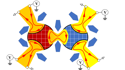
Figure 2: Schematic of a strong coupling between two charge Kondo circuits. Notations are the same as on Figure 1 with two distinct differences: i) different color scheme used for the left (orange, hot) and right (yellow, cold) parts of the circuit; ii) the central part of the system is modified. The tunnel contact in the center of Fig 1 is replaced by almost transparent QPC. The chiral edge mode strongly couples QD1 and QD2. The temperature gradient (shown by continuous change of colour from orange to yellow) is applied across the central QPC.

The investigation of TP for the weak coupling between two CKCs in both cases: 1CK - 2CK and 2CK - 2CK shows the competition between the FL and NFL picture. However, the windows of parameters to observe the FL property are much broader than the windows to access the NFL one. The reason is that the NFL intermediate coupling fixed points of MCK are hyperbolic and therefore unstable. The results of this work not only cover the perturbative accessible regimes, which have been represented in Ref. thanh2018 , but also show a rich property of the TP in different domains of parameters.

Extending the proposal of the weak coupling between two CKCs thanh2018 to the regime of almost transparent QPC in the central area of the DCKC, the very recent experiment Gordon2023 and theory Karki2022 ; Z3_DCK have investigated the strong coupling limit. Let us comment on the connection between the weak and strong coupling regimes of the DCKCs. In Ref. thanh2018 we have considered the DCKC weakly connecting 1CK-1CK or 1CK-2CK or 2CK-2CK. The same realization for the strong coupling of two Kondo simulators has also been theoretically suggested in thanh2018 and experimentally realized recently in Gordon2023 for 1CK-1CK coupling com2 . One of the most exciting theoretical predictions of the two-impurity single channel Kondo effect Jones_Varma ; Gan_95 ; Logan2012 is a possibility to map the model under certain assumptions onto the 2CK Hamiltonian. Interestingly, the Refs. Gordon2023 ; Karki2022 ; Z3_DCK showed that at the triple degeneracy point of the DCKC $Z_{3}$ symmetry and corresponding local parafermion emerge. It is straightforward to extend the idea thanh2018 to MCK-NCK strong coupling (see Fig 2). Suppose that there are $M>1$ identical QPCs in the left hand side of the DCKC and $N>1$ identical QPCs in the right side of it. The total degeneracy is $M+1+N$ and corresponding emergent local symmetry is $Z_{M+N+1}$. There are three important $(M,N)$ realizations accessible through existing experimental setups: i) $(2,1)$ or $(1,2)$ connecting 1CK and 2CK with emergent symmetry $Z_{4}$; ii) $(2,2)$ and iii) $(3,1)$ or $(1,3)$ with emergent symmetry $Z_{5}$. Corresponding weak link setups are characterized by the symmetries: i) $U(1)\times Z_{2}$; ii) $Z_{2}\times Z_{2}$ and iii) $U(1)\times Z_{3}$. As the weak coupling regimes of ii) and iii) are clearly distinct, being characterized by both different symmetries and different Lorenz ratios (see Ref. Kis2023 for more details), it is interesting to examine regimes ii) and iii) in the strong coupling limit. In particular it is important to understand the symmetry of local parafermion emerging in the strong link setup. In addition, switching between different intermediate coupling fixed points results in crossovers between various fractionalized modes manifesting itself in distinctly different regimes of the charge and heat transport.

The weak link regime discussed in this manuscript was analysed using a standard approach based on the transport integrals thanh2018 . The validity of this approach is justified by an assumption that both temperature and voltage drops occur exactly at the central tunnel barrier. As a result, both the left and the right parts of the DCKC are considered at thermal and mechanical equilibrium being characterized by certain temperature $T$ and chemical potential $\mu$. This approach is clearly invalid for the strong link between two sides of the Kondo simulator where both the temperature and the voltage changes continuously across the central QPC. The full-fledged linear response theory of the charge and heat transport across the strong link of the two-site Kondo simulators can be constructed by using Luttinger’s pseudo-gravitational approach lut1 ; lut2 or thermo-mechanical potential lut3 ; lut4 method in combination with Kubo equations. The theory beyond linear response requires also using Keldysh formalism lut3 ; lut4 and represents an interesting and important direction for the future investigation.

VI Conclusion

In this work, we revisited the thermoelectric transport at the weak link of the DCKC model proposed in the Ref. thanh2018 . The Abelian bosonization approach is used for both 1CK and 2CK setup while the refermionization technique is applied in order to solve the 2CK model nonperturbatively. We show the different windows of the parameter set where the TP behaves either the full FL or NFL characteristics or the competition between these properties. The nonperturbative results not only cover the perturbative results but also be applicable in the lower temperature regime $T<|r_{j}|^{2}E_{C,j}$. We predict that the TP is enhanced in the DCKC in comparison with the single CKC setup. Indeed, a complex charge Kondo circuit which shows the diversity of the competition between the FL and NFL properties, can be a potential thermoelectric material. Moreover, we propose to use the experimental implementation in Ref. Gordon2023 for investigating the different parafermion contributions to the quantum thermoelectricity when the coupling between QDs is switched from weak to strong.

Appendix

In this Appendix we represent the details of the different approaches at different limits in order to obtain the results shown in the Subsection V.2.

1, If $p_{1}\rightarrow 0,p_{2}\rightarrow 0$, we have:

$$\lim_{p_{1}\rightarrow 0}\frac{p_{1}}{\left(z+\frac{u}{2}\right)^{2}+p_{1}^{2}} =\pi\delta\left(z+\frac{u}{2}\right),$$ (47)

$$\lim_{p_{2}\rightarrow 0}\frac{p_{2}}{\left(z-\frac{u}{2}\right)^{2}+p_{2}^{2}} =\pi\delta\left(z-\frac{u}{2}\right).$$ (48)

As a result

$$\lim_{p_{2}\rightarrow 0}\frac{F_{T,m}\left(p_{1}\rightarrow 0,p_{2}\right)}{p_{2}}$$

$$=\lim_{p_{2}\rightarrow 0}\int_{-\infty}^{\infty}du\frac{\pi u^{3}\left[u^{2}+4\pi^{2}\right]}{\sinh\left[u\right]\left[u^{2}+p_{2}^{2}\right]}$$

$$=\int_{-\infty}^{\infty}du\frac{\pi u\left[u^{2}+4\pi^{2}\right]}{\sinh\left[u\right]}=\frac{3\pi^{5}}{4},$$ (49)

and, finally

$$\lim_{p_{1}\rightarrow 0}\frac{F_{T,s}\left(p_{1},p_{2}\rightarrow 0\right)}{p_{1}}=\frac{3\pi^{5}}{4}~{}.$$ (50)

We obtain the electric conductance as

$$G^{\left(0\right)} =\frac{\pi^{2}G_{C}T^{2}}{6\gamma^{2}E_{C,1}E_{C,2}},$$ (51)

and the thermoelectric coefficient as

$$\!\!\!\!G_{T}^{(1)}=-\frac{\pi^{4}G_{C}T^{2}}{32e\gamma E_{C,1}E_{C,2}}\left[|r_{1}|^{2}\ln\left(\frac{E_{C,1}}{T}\right)\sin\left(2\pi N_{1}\right)\right.$$

$$\left.+|r_{2}|^{2}\ln\left(\frac{E_{C,2}}{T}\right)\sin\left(2\pi N_{2}\right)\right].$$ (52)

2, If $p_{1}\rightarrow 0,p_{2}\gg 1$ we have:

$$F_{C}\left(p_{1}\rightarrow 0,p_{2}\right)=\int_{-\infty}^{\infty}du\frac{\pi p_{2}u\left[u^{2}+4\pi^{2}\right]}{\sinh\left[u\right]\left[u^{2}+p_{2}^{2}\right]},$$

$$\!\!\!\!\!\!\!\!F_{C}\left(p_{1}\rightarrow 0,p_{2}\gg 1\right)\!=\!\frac{\pi}{p_{2}}\!\!\int_{-\infty}^{\infty}\!\!\!\!\!\!du\frac{u\left[u^{2}+4\pi^{2}\right]}{\sinh\left[u\right]}\!=\!\frac{9\pi^{5}}{4p_{2}},$$ (53)

and

$$\!\!\!\!\!\!\!\!F_{T,m}\left(p_{1}\rightarrow 0,p_{2}\gg 1\right)\!=\!\frac{\pi}{p_{2}}\!\!\int_{-\infty}^{\infty}\!\!\!\!\!\!\!du\frac{u^{3}\left[u^{2}+4\pi^{2}\right]}{\sinh\left[u\right]}\!=\!\frac{3\pi^{7}}{2p_{2}}.$$ (54)

The calculation of the $F_{T,s}$ is a bit complicated, which concerns the principal value (PV) as follows.

$$\!\!\!\!\frac{F_{T,s}\left(p_{1}\rightarrow 0,p_{2}\gg 1\right)}{p_{1}}=\frac{1}{p_{2}}\text{PV}\int_{-\infty}^{\infty}\!\!\!\!dz\int_{-\infty}^{\infty}\!\!\!\!du$$

$$\!\!\!\!\times\frac{uz\left[u^{2}+4\pi^{2}\right]}{\left(z+\frac{u}{2}\right)\sinh\left(\frac{u}{2}\right)\left[\cosh\left(z\right)+\cosh\left(\frac{u}{2}\right)\right]}$$

$$\!\!\!\!\!\!=\frac{8}{p_{2}}\!\!\int_{-\infty}^{\infty}\!\!\!\!dp\!\int_{-\infty}^{\infty}\!\!\!\!dq\left\{\frac{q\left[q^{2}+4\pi^{2}\right]}{\sinh\left(q\right)\cosh\left(p/2\right)\cosh\left(p/2-q\right)}\right.$$

$$\!\!\!\!\left.-\frac{\tanh\left(p/2\right)q^{2}\left[q^{2}+4\pi^{2}\right]}{p\cosh\left(p/2+q\right)\cosh\left(p/2-q\right)}\right\}=\frac{192\pi^{4}}{25p_{2}}.$$ (55)

The electric conductance $G$ and the thermoelectric coefficient $G_{T}$ is computed at the first non-zero term in the nonperturbative treatment are

$$G^{\left(0\right)}=\frac{3G_{C}\pi^{5}T^{3}}{32\gamma^{2}\Gamma_{2}E_{C,1}E_{C,2}},$$ (56)

$$\!\!\!\!G_{T}^{(1)}=-\frac{8G_{C}\pi^{3}T^{3}}{25e\gamma E_{C,1}E_{C,2}\Gamma_{2}}\left[|r_{1}|^{2}\ln\left(\frac{E_{C,1}}{T}\right)\sin\left(2\pi N_{1}\right)\right.$$

$$\left.+\frac{25\pi^{3}}{128}\frac{T}{\Gamma_{2}}|r_{2}|^{2}\ln\left(\frac{E_{C,2}}{\Gamma_{2}}\right)\sin\left(2\pi N_{2}\right)\right].$$ (57)

3, $p_{1}\gg 1,p_{2}\rightarrow 0$: This limit is opposite to the second limit. The calculation process is the same as the above one.

$$F_{C}\left(p_{1}\gg 1,p_{2}\rightarrow 0\right)$$

$$=\frac{\pi}{p_{1}}\int_{-\infty}^{\infty}du\frac{u\left[u^{2}+4\pi^{2}\right]}{\sinh\left[u\right]}=\frac{9\pi^{5}}{4p_{1}},$$ (58)

$$\frac{F_{T,m}\left(p_{1}\gg 1,p_{2}\rightarrow 0\right)}{p_{2}}=\frac{1}{p_{1}}\text{PV}\int_{-\infty}^{\infty}dz\int_{-\infty}^{\infty}du$$

$$\times\frac{uz\left[u^{2}+4\pi^{2}\right]}{\left(z-\frac{u}{2}\right)\sinh\left(\frac{u}{2}\right)\left[\cosh\left(z\right)+\cosh\left(\frac{u}{2}\right)\right]}=\frac{192\pi^{4}}{25p_{1}},$$ (59)

$$F_{T,s}\left(p_{1}\gg 1,p_{2}\rightarrow 0\right) =\frac{3\pi^{7}}{2p_{1}}.$$ (60)

The electric conductance is

$$G^{\left(0\right)}=\frac{3G_{C}\pi^{5}T^{3}}{32\gamma^{2}E_{C,1}E_{C,2}\Gamma_{1}},$$ (61)

and the thermoelectric coefficient is

$$G_{T}^{(1)}=-\frac{8G_{C}\pi^{3}T^{3}}{25e\gamma E_{C,1}E_{C,2}\Gamma_{1}}$$

$$\times\left\{\frac{25\pi^{3}}{128}\frac{T}{\Gamma_{1}}|r_{1}|^{2}\ln\left(\frac{E_{C,1}}{\Gamma_{1}}\right)\sin\left(2\pi N_{1}\right)\right.$$

$$+\left.|r_{2}|^{2}\ln\left(\frac{E_{C,2}}{T}\right)\sin\left(2\pi N_{2}\right)\right\}.$$ (62)

4, If $p_{1}\gg 1,p_{2}\gg 1$, we simply remove the terms which are summed with $p_{1}^{2}$ and $p_{2}^{2}$ in the denominator of the formula (37). We then obtain:

$$F_{C}\left(p_{1}\gg 1,p_{2}\gg 1\right)=\frac{1}{p_{1}p_{2}}\int_{-\infty}^{\infty}dz\int_{-\infty}^{\infty}du$$

$$\times\frac{u\left[u^{2}+4\pi^{2}\right]}{\sinh\left[\frac{u}{2}\right]\left[\cosh\left(z\right)+\cosh\left(\frac{u}{2}\right)\right]}=\frac{64\pi^{4}}{5p_{1}p_{2}}.$$ (63)

$$F_{T,m}\left(p_{1}\gg 1,p_{2}\gg 1\right)=\frac{1}{p_{1}p_{2}}\int_{-\infty}^{\infty}dz\int_{-\infty}^{\infty}du$$

$$\times\frac{\left(z-\frac{u}{2}\right)uz\left[u^{2}+4\pi^{2}\right]}{\sinh\left[\frac{u}{2}\right]\left[\cosh\left(z\right)+\cosh\left(\frac{u}{2}\right)\right]}=\frac{192\pi^{6}}{35p_{1}p_{2}}.$$ (64)

$$F_{T,s}\left(p_{1}\gg 1,p_{2}\gg 1\right)=\frac{1}{p_{1}p_{2}}\int_{-\infty}^{\infty}dz\int_{-\infty}^{\infty}du$$

$$\times\frac{\left(z+\frac{u}{2}\right)uz\left[u^{2}+4\pi^{2}\right]}{\sinh\left[\frac{u}{2}\right]\left[\cosh\left(z\right)+\cosh\left(\frac{u}{2}\right)\right]}=\frac{192\pi^{6}}{35p_{1}p_{2}}.$$ (65)

The electric conductance and the thermoelectric coefficient in this limit are

$$G=\frac{8G_{C}\pi^{4}T^{4}}{15\gamma^{2}E_{C,1}E_{C,2}\Gamma_{1}\Gamma_{2}},$$ (66)

$$G_{T}^{(1)}=-\frac{24G_{C}\pi^{5}T^{5}}{105e\gamma E_{C,1}E_{C,2}\Gamma_{1}\Gamma_{2}}$$

$$\times\left\{\frac{|r_{1}|^{2}}{\Gamma_{1}}\ln\left(\frac{E_{C,1}}{T+\Gamma_{1}}\right)\sin\left(2\pi N_{1}\right)\right.$$

$$+\left.\frac{|r_{2}|^{2}}{\Gamma_{2}}\ln\left(\frac{E_{C,2}}{T+\Gamma_{2}}\right)\sin\left(2\pi N_{2}\right)\right\}.$$ (67)

References

• (1) G. Snyder and E. Toberer, Nat. Mater. 7, 105 (2008).
• (2) T. J. Seebeck, Abh. Akad. Wiss. Berlin 1820-21, 289 (1822).
• (3) J. F. Li, W.S. Liu, L.D. Zhao, and M. Zhou, NPG Asia Mater. 2, 152 (2010).
• (4) Y. Du, K. F. Cai, S. Chen, H. Wang, S. Z. Shen, R. Donelson, and T. Lin, Sci. Rep. 5, 6144 (2015).
• (5) M. S. Dresselhaus, G. Chen, M. Y. Tang, R. G. Yang, H. Lee, D. Z. Wang, Z. F. Ren, J. P. Fleurial, P. Gogna, Adv. Mater. 19, 1043 (2007).
• (6) G. Chen,M. S. Dresselhaus, G. Dresselhaus, J. P. Fleurial, and T. Caillat, Int. Mater. Rev. 48, 45 (2003).
• (7) Y. M. Blanter and Y. V. Nazarov, Quantum Transport: Introduction to Nanoscience (Cambridge University Press, Cambridge, 2009).
• (8) K. Kikoin, M. N. Kiselev, and Y. Avishai, Dynamical Symmetry for Nanostructures. Implicit Symmetry in Single-Electron Transport Through Real and Artificial Molecules (Springer, New York, 2012).
• (9) A. A. M. Staring, L. W. Molenkamp, B. W. Alphenhaar, H. van Houten, O. J. A. Buyk, M. A. A. Mabesoone, C. W. J. Beenakker, and C. T. Foxon, Europhys. Lett. 22, 57 (1993).
• (10) M. Turek and K. A. Matveev, Phys. Rev. B 65, 115332 (2002).
• (11) K. Flensberg, Phys. Rev. B 48, 11156 (1993).
• (12) K. A. Matveev, Phys. Rev. B 51, 1743 (1995).
• (13) A. Furusaki and K. A. Matveev, Phys. Rev. Lett. 75, 709 (1995).
• (14) A. V. Andreev and K. A. Matveev, Phys. Rev. Lett. 86, 280 (2001); Phys. Rev. B 66, 045301 (2002).
• (15) K. Le Hur, Phys. Rev. B 64, 161302(R) (2001).
• (16) K. Le Hur and G. Seelig, Phys. Rev. B 65, 165338 (2002).
• (17) J. Kondo, Prog. Theor. Phys. 32, 37 (1964).
• (18) A. Hewson, The Kondo Problem to Heavy Fermions (Cambridge University Press, Cambridge, England, 1993).
• (19) A. M. Tsvelik and P. B. Wiegmann, Adv. in Phys., 32, 453 (1983).
• (20) N. Andrei, K. Furuya, and J. H. Lowenstein, Rev. Mod. Phys. 55, 331 (1983).
• (21) L. Kouwenhoven and L. I. Glazman, Phys. World 14, 33 (2001).
• (22) R. Scheibner, H. Buhmann, D. Reuter, M. N. Kiselev, and L. W. Molenkamp, Phys. Rev. Lett. 95, 176602 (2005).
• (23) T. K. T. Nguyen, M. N. Kiselev, and V. E. Kravtsov, Phys. Rev. B 82, 113306 (2010).
• (24) T. K. T. Nguyen and M. N. Kiselev, Phys. Rev. B 92, 045125 (2015).
• (25) T. K. T. Nguyen, M. N. Kiselev, Phys. Rev. B 97, 085403 (2018).
• (26) A. V. Parafilo, T. K. T. Nguyen, and M. N. Kiselev, Phys. Rev. B 105, L121405 (2022).
• (27) T. K. T. Nguyen and M. N. Kiselev, Commun. Phys. 32, 331 (2022).
• (28) A. V. Parafilo and T. K. T. Nguyen, Commun. Phys. 33, 1 (2023).
• (29) M. N. Kiselev, arXiv: 2304.10872 (2023).
• (30) E. Sela, A. K. Mitchell, and L. Fritz, Phys. Rev. Lett. 106, 147202 (2011).
• (31) A. K. Mitchell, L. A. Landau, L. Fritz, and E. Sela, Phys. Rev. Lett. 116, 157202 (2016).
• (32) L. A. Landau, E. Cornfeld, and E. Sela, Phys. Rev. Lett. 120, 186801 (2018).
• (33) G. A. R. van Dalum, A. K. Mitchell, and L. Fritz, Phys. Rev. B 102, 041111(R) (2020).
• (34) T. K. T. Nguyen and M. N. Kiselev, Commun. Phys. 30, 1 (2020).
• (35) T. K. T. Nguyen, A. V. Parafilo, H. Q. Nguyen, and M. N. Kiselev, Phys. Rev. B 107, L201402 (2023).
• (36) Z. Iftikhar, S. Jezouin, A. Anthore, U. Gennser, F. D. Parmentier, A. Cavanna and F. Pierre, Nature 526, 233 (2015).
• (37) Z. Iftikhar, A. Anthore, A. K. Mitchell, F. D. Parmentier, U. Gennser, A. Ouerghi, A. Cavanna, C. Mora, P. Simon, and F. Pierre, Science 360, 1315 (2018).
• (38) Ph. Nozières and A. Blandin, J. Phys. 41, 193 (1980).
• (39) D. Cox and A. Zawadowski, Advances in Physics 47, 599 (1998).
• (40) I. Affleck and A. W. W. Ludwig, Phys. Rev. B 48, 7297 (1993).
• (41) N. Andrei and C. Destri, Phys. Rev. Lett. 52, 364 (1984).
• (42) M. Fabrizio, A. O. Gogolin, and P. Nozières, Phys. Rev. Lett. 74, 4503 (1995).
• (43) M. Fabrizio, A. O. Gogolin, and P. Nozières, Phys. Rev. B 51, 16088 (1995).
• (44) A. O. Gogolin, A. A. Nersesyan, and A. M. Tsvelik, Bosonization Approach to Strongly Correlated Systems (Cambridge University Press, Cambridge, England, 1998).
• (45) V. J. Emery and S. Kivelson, Phys. Rev. B 46, 10812 (1992).
• (46) A. B. Zamolodchikov and V. A. Fateev, ZhETF 89, 380 (1985) [Sov. Phys. JETP 62, 215 (1985)].
• (47) H. Yi and C. L. Kane, Phys. Rev. B 57, R5579 (1998).
• (48) H. Yi, Phys. Rev. B 65, 195101 (2002).
• (49) I. Affleck, M. Oshikawa, and H. Saleur, Nucl. Phys. B 594, 535 (2001).
• (50) C. Nayak, S. H. Simon, A. Stern, M. Freedman, and S. D. Sarma, Rev. Mod. Phys. 80, 1083 (2008).
• (51) J. Alicea and P. Fendley, Annu. Rev. Condens. Matter Phys. 7, 119 (2016).
• (52) T. K. T. Nguyen and M. N. Kiselev, Phys. Rev. Lett. 125, 026801 (2020).
• (53) W. Pouse, L. Peeters, C. L. Hsueh, U. Gennser, A. Cavanna, M. A. Kastner, A. K. Mitchell, and D. Goldhaber-Gordon, Nat. Phys. (2023).
• (54) D. B. Karki, E. Boulat, and C. Mora, Phys. Rev. B 105, 245418 (2022).
• (55) D. B. Karki, E. Boulat, W. Pouse, D. Goldhaber-Gordon, A. K. Mitchell, and C. Mora, Phys. Rev. Lett. 130, 146201 (2023).
• (56) I. L. Aleiner and L. I. Glazman, Phys. Rev. B 57, 9608 (1998).
• (57) T. Giamarchi, Quantum Physics in One Dimension (Oxford University Press, Oxford, UK, 2003).
• (58) There is a missing factor $2\pi$ in Eq. (13) of Ref. thanh2018 , which consequently requires to put an additional prefactor $2\pi$ in all formulas of thermoelectric coefficient $G_{T}$ and thermopower $S$ thereafter.
• (59) Historically, the idea of Double-Large-Dot Charge Kondo configuration has been first theoretically proposed in LeHur3 for the thermodynamic investigation of the fractional $e/2$ charge Coulomb Blockade capacitance peaks.
• (60) K. Le Hur, Phys. Rev. B 67, 125311 (2003).
• (61) B. A. Jones and C. M. Varma, Phys. Rev. Lett. 58, 843 (1987); B. A. Jones, C. M. Varma, and J. W. Wilkins, ibid. 61, 125 (1988).
• (62) J. Gan, Phys. Rev. Lett. 74, 2583 (1995); Phys. Rev. B 51, 8287 (1995).
• (63) A. K. Mitchell, E. Sela, and D. E. Logan, Phys. Rev. Lett. 108, 086405 (2012).
• (64) J. M. Luttinger, Phys. Rev. 135, A1505 (1964).
• (65) B. S. Shastry, Rep. Prog. Phys. 72, 016501 (2009).
• (66) F. G. Eich, M. Di Ventra, and G. Vignale Phys. Rev. Lett. 112, 196401 (2014).
• (67) F. G. Eich, A. Principi, M. Di Ventra, and G. Vignale Phys. Rev. B 90, 115116 (2014).