Automated Machine Learning for Remaining Useful Life Predictions

Abstract

Being able to predict the remaining useful life (RUL) of an engineering system is an important task in prognostics and health management. Recently, data-driven approaches to RUL predictions are becoming prevalent over model-based approaches since no underlying physical knowledge of the engineering system is required. Yet, this just replaces required expertise of the underlying physics with machine learning (ML) expertise, which is often also not available. AutoML promises to build end-to-end ML pipelines automatically enabling domain experts without ML expertise to create their own models. This paper introduces AutoRUL, an automated machine learning (AutoML)-driven end-to-end approach for automatic RUL predictions. AutoRUL combines fine-tuned standard regression methods to an ensemble with high predictive power. By evaluating the proposed method on eight real-world and synthetic datasets against state-of-the-art hand-crafted models, we show that AutoML provides a viable alternative to hand-crafted data-driven RUL predictions. Consequently, creating RUL predictions can be made more accessible for domain experts using AutoML by eliminating ML expertise from data-driven model construction.

I Introduction

In recent manufacturing, a reliable, available, and sustainable production of goods is important to be competitive. This requires advanced maintenance strategies such as predictive maintenance. Traditional strategies such as corrective or preventive maintenance cause unplanned downtime or do not utilize existing resources completely due to superfluous maintenance actions. Predictive maintenance can help to avoid unplanned downtime while also reducing unnecessary maintenance costs. Knowledge about the future degradation behavior of an engineering system (ES) is crucial to plan the required maintenance as predictive maintenance is becoming more important in industry. The engineering discipline of prognostics and health management (PHM) studies techniques for transitioning from corrective or preventive maintenance to predictive maintenance. A key task in PHM is the prognosis of the remaining useful life (RUL). Approaches are often divided into model-based, data-driven, and hybrid methods [1]. Usually, the RUL is used to plan the next maintenance and has attracted considerable interest in the research community.

Model-based approaches use mathematical descriptions, like algebraic and differential equations or physics-based models to predict the future degradation behavior of a system [2]. Such models require thorough understanding of the mechanism involved in the degradation process and are time-consuming to create. Also, not all systems can be expressed with sufficient precision in solvable mathematical or physics models due to the complexity of real world systems [3]. With the integration of more sensors, the amount of available data about the condition of a system is gradually increasing. In parallel, machine learning (ML) has matured and achieved wide-spread dissemination. Similarly, data-driven models for RUL have become more popular. By using ML to model the relationship of the system health and RUL, no thorough understanding of the degradation process is required. In recent years, various ML methods, like random forest or different neural networks, have been proposed to model RUL predictions [2, 4].

Yet, to actually create data-driven models for RUL predictions from recorded sensor data, specialized knowledge in data modeling and ML is necessary. For small and medium-sized enterprises such knowledge is often not available. As a consequence, the potential of data-driven methods is rarely utilized. AutoML promises to enable domain experts, i.e., the manufacturer of an ES, to develop data-driven ML methods for RUL prediction without detailed knowledge of ML [5]. Enterprises with ML knowledge can benefit from AutoML by automating time-consuming ML sub-tasks, leading to lower costs and higher competitiveness.

The contributions of this paper are as follows:

1. We propose a universal end-to-end AutoML solution, called AutoRUL, for RUL predictions for domain experts that does not require ML knowledge.

2. We compare the traditional manual creation of RUL predictions with the proposed automatic approach.

3. AutoRUL is validated against five state-of-the-art RUL models on a wide range of real-world and synthetic datasets. This is the first evaluation of a single AutoML tool on a wide variety of RUL datasets.

4. In the spirit of reproducible research, all source code and used datasets are publicly available.

Section II introduces related work. Our proposed approach is introduced in Section III and compared in Section IV. In Section V the proposed method is validated on RUL datasets. The paper concludes in a short discussion in Section VI.

II Related Work

II-A Remaining Useful Life Prognosis

Key tasks in PHM are the fault detection, diagnosing which component of an ES causes a present fault condition, the health assessment, and the prognosis of the RUL of a system [2]. Each prognosis approach requires—or at least benefits from—the availability of sufficient condition data of the system. The knowledge of future degradation behavior and RUL is crucial for maintenance strategies such as predictive maintenance.

RUL prediction can be described as estimating the remaining time duration that an ES is likely to continue to operate before maintenance is required or a failure occurs [3]. There are two main strategies, indirect and direct, for predicting RUL using a data-driven model [6]. Indirect RUL prognosis first predicts future degradation behavior. At the time of prediction, the model performs an extrapolation based on present condition data until a failure criterion is achieved. The time span of this extrapolation corresponds to the actual predicted RUL. In contrast, in the direct approach, the RUL is predicted directly given the current condition data. This requires models determining the correlation between condition data and RUL based on a defined failure criterion. In this paper, we consider a direct data-driven RUL prognosis.

More formally, data-driven RUL predictions is formulated as a sequence-to-target learning problem aiming to learn a mapping $h:\mathcal{X}\rightarrow\mathcal{Y}$ from historical condition data $\vec{x}\in\mathcal{X}$—recorded over various instances, i.e., ESs—to the RUL $y\in\mathcal{Y}\subset\mathds{R}$. Each instance $\vec{x}_{i}$ contains a $d=|\vec{x}_{i}|$ dimensional (multivariate) time series of arbitrary length with sensor data from the system setup until the defined failure criterion. Training data is defined as $\mathcal{D}_{\mathrm{train}}=\{(\vec{x}_{i},y_{i})\}_{i=1}^{N}$ with $N$ being the number of instances. Test data $\mathcal{D}_{\mathrm{test}}=\{(\vec{x}^{\prime}_{i},y^{\prime}_{i})\}_{i=1}^{M}$ contain sensor data up to some time $T_{i}$ with $y_{i}$ being the corresponding RUL that is left after $T_{i}$. A loss function $\mathcal{L}$ is used to measure the performance of $h$ on $\mathcal{D}_{\mathrm{test}}$. In the context of RUL, loss functions can be divided into general symmetric loss functions or specialized asymmetric loss functions. We use the root mean square error (RMSE)

$$\mathcal{L}_{\mathrm{RMSE}}\left(h,\mathcal{D}_{\mathrm{test}}\right):=\sqrt{\dfrac{1}{M}\sum_{i=1}^{M}\bigl{(}h(\vec{x}^{\prime}_{i})-y^{\prime}_{i}\bigr{)}^{2}}$$ (1)

with $h(\vec{x}^{\prime}_{i})$ being the predicted RUL on $\vec{x}^{\prime}_{i}$ in this work, but any other loss function for regression would also be applicable.

II-B Human Expert Approach

The elementary phases in developing an ML model for RUL predictions are similar to developing a model for regressions, namely data pre-processing, feature engineering, and the ML model development. Yet, expert knowledge regarding RUL prognosis as well as the ES can be used to integrate additional information into the respective phases [3].

II-B1 Data Pre-Processing

Basis for prediction models are historical raw signals recorded by various sensors of the respective ESs. Typically, these signals contain shortcomings, e.g., noise [2, 1]. Therefore, signal processing methods, like smoothing or imputation, are used to increase the data quality. In addition, different methods can be applied to subsequently generate informative features that enable the RUL to be mapped, e.g., the generation of a frequency spectrum [7].

II-B2 Feature Engineering

Next, new meaningful features from the pre-processed signals are generated [1]. This is crucial for the later modelling. Often, new features are generated on shorter time windows containing only a few measurements. They can be grouped into common—like statistical time-domain features—, specific—developed specifically for an individual ES—and ML-based—based on anomaly detection or one-class classification [8]—health indicators [7, 8]. In addition, features taking operating conditions, e.g., loading, into account are also essential. Finally, relevant features must be selected considering the correlation of the features with the target RUL. Statistical hypothesis tests are often used for this [9]. In case of too many relevant features, methods like autoencoders or PCA are used for dimension reduction [10].

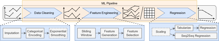
Figure 1: Schematic representation of pipelines constructed by AutoRUL to map sensor data to RUL predictions. The pipeline is structured into three major phases: data cleaning, feature engineering and regression. Each phase contains multiple steps, displayed below the ML pipeline, configured by various hyperparameters. Steps with solid borders indicate mandatory steps included in every pipeline while dashed borders represent optional pipeline steps.

II-B3 ML Model Development

Selecting the best ML method for the ES or condition data is a challenging task and requires sufficient ML expertise. Various ML methods like support vector machine (SVM) [11], random forest (RF) [12], and different neural networks are therefore available [2, 4]. Versatile adaptations of such methods to the respective ESs or requirements can be found in the literature [2, 3]. NNs, for example, allow many adaptation options to the system through different network architectures. Recently, several specialized network architectures have been proposed [2, 3]. Mo et al. [13] proposed a transformer encoder-based model with an improved sensitivity for local contexts (time steps). Shi and Chehade [14] introduced a dual long short-term memory (LSTM) framework for combining the detection of health states with the RUL prediction for achieving better performance. Wang et al. [15] proposed a combination of an autoencoder for feature extraction and a convolutional neural network (CNN) for RUL prediction.

This brief overview illustrates that numerous adaptations of a selected ML method are possible. Especially the integration of additional expert knowledge about the ES allows improving the prediction performance [16, 17].

II-C Automated Machine Learning

AutoML aims to construct ML pipelines automatically with minimal human interaction [5]. Many different AutoML approaches have been proposed with most propositions focusing on standard learning tasks, e.g., tabular or image classification. Virtually all AutoML approaches model the synthesis of ML pipelines as a black-box optimization problem: Given a dataset and loss function, AutoML searches for a pipeline in a predefined search space $\Lambda$ minimizing the validation loss.

In general, various AutoML tools for standard regression and time-series forecasting tasks exist. Yet, nearly all of these tools are of limited use for RUL predictions due to two limitations: 1. Tools for standard regression assume tabular data and do not provide measures to transform time-series data into a tabular format. 2. Tools for time-series forecasting train local statistical models that can forecast the future behavior of a single ES without learning generalized concepts over multiple system instances.

More recently, dedicated AutoML systems for RUL predictions have been proposed. ML-Plan-RUL [18] was the first AutoML tool tailored to RUL predictions. Using descriptive statistics, the time series data is transformed to fixed, tabular data suitable for standard regression. In a follow-up work, the search space of ML-Plan-RUL is split into a feature engineering and regression part. By using a joint genetic algorithm over both search spaces, the improved approach, named AutoCoevoRUL [19], was able to outperform ML-Plan-RUL. Similarly, Singh et al. [20] used a genetic algorithm to optimize the parameters of an LSTM to predict the RUL of batteries. Finally, Zhou et al. [21] used a combination of LSTM and CNN cells for RUL predictions with the exact network architecture being determined using AutoML.

III Automated Remaining Useful Life Predictions

AutoML frameworks usually consider a combined search space covering all necessary steps to assemble an ML pipeline for a specific task. The search space covers both the selection of specific algorithms, e.g., using an SVM for regression, as well as the configuration of the selected algorithms via hyperparameters. Considering the task of RUL prediction, a complete ML pipeline has to be able to consume the raw sensor data as univariate or multivariate time series, pre-process the data and finally use a regression algorithm to create RUL predictions. In contrast to standard regression tasks, which assume tabular input data, the pipeline either has to include methods to transform time series into tabular data, or the regression algorithm has to be capable of consuming time series data directly, like, for example, LSTMs.

Our approach, AutoRUL, uses a flexible best-practice pipeline, inspired by human experts, displayed in Fig. 1. It starts with basic data cleaning, followed by a feature generation step and an optional transformation into tabular data if necessary. A regressor is used to predict the RUL. AutoML aims to fill these generic pipeline steps with actual algorithms, configured by respective hyperparameters, such that the loss function (1) is minimized on a validation dataset $\mathcal{D}_{\mathrm{val}}$. The according optimization problem is formulated as

$$\vec{\lambda}^{*}\in\operatorname*{arg\,min\;}_{\vec{\lambda}\in\Lambda}\mathcal{L}_{\mathrm{RMSE}}\left(h_{\vec{\lambda}},\mathcal{D}_{\mathrm{val}}\right)$$ (2)

with $h_{\vec{\lambda}}$ being the pipeline defined by the configuration $\vec{\lambda}$, i.e., a set of selected algorithms and hyperparameters. To actually solve (2), we use Bayesian optimization, namely SMAC [22]. Bayesian optimization is an iterative optimization procedure for expensive objective functions. By repeatedly sampling pipeline candidates, an internal surrogate model of the objective function is constructed. This surrogate model is used to trade-off exploration of under-explored settings and exploitation of well-performing regions.

The search space $\Lambda$ of AutoRUL allows the creation of $624$ unique pipelines which can be further configured by a total of $168$ hyperparameters. In the remainder of this section, further details regarding the search space definition as well as implemented performance improvements are presented. Further information are available in the online appendix.

Data Cleaning

The first part of the generated ML pipeline is dedicated to data cleaning to solve common data issues. At first, missing values for individual timestamps are always imputed, with the actual imputation method, e.g., repeating neighbouring values or using the sequence mean value, being selected by the optimizer. Next, categorical variables are encoded to ensure compatibility with all later steps. Finally, an optional exponential smoothing of the data can be applied.

Feature Engineering

Next, the raw sensor measurements are enriched with new features. Using a sliding window with tunable length $\lambda_{w}$, a context with prior observations is created for each timestamp $t$. Especially for high-frequent measurements, not every recording is relevant but increases the computational load. A configurable stride hyperparameter $\lambda_{s}$ is used to determine the number of steps the window is shifted, effectively down-sampling $\vec{x}_{i}$. By design $\lambda_{s}$ is always smaller than $\lambda_{w}$ leading to an overlap of adjacent windows.

In general, two different approaches are used to create new features from the generated windows: 1. The $d\times\lambda_{w}$ measurements in a single window can be flattened to a $1\times(d\cdot\lambda_{w})$ vector to embed lagged observations. 2. Each generated window can be interpreted as new time series with fixed length $\lambda_{w}$. The new time series can be characterized using different statistical and stochastic features. AutoRUL supports $43$ unique features and the optimizer can select which features to include. In both cases the time series characteristics of the input data is preserved. During feature selection, irrelevant features are identified using statistical hypothesis tests to eliminate features uncorrelated with the regression target [9].

Regression

The actual RUL predictions are created by mapping the problem to a regression learning task. In contrast to other RUL publications, we do not aim to propose a novel method for RUL predictions, but instead focus on configuring and combining standard ML regression models to achieve a good performance on a wide variety of datasets.

Recently, various sequence-to-sequence (seq2seq) models that consume the complete input sequence and produce a new sequence, i.e., the RUL, have been proposed for RUL predictions. AutoRUL supports recurrent architectures, namely LSTM and gated recurrent unit (GRU), and convolutional architectures, namely CNN and temporal convolutional network (TCN). For each basis architecture, the concrete network architecture, like the size of latent spaces or number of layers, is configured via hyperparameters. In addition, the complete training process of the NN, e.g., the batch size or learning rate, is tunable via various hyperparameters.

Alternatively, AutoRUL supports splitting $\vec{x}_{i}$ into chunks with fixed length, effectively transforming variable length input data into a tabular format with fixed dimensions. This allows employing traditional regression methods like RFs.

Performance Improvements

Even though Bayesian optimization is quite efficient in the number of sampled configurations, AutoML still evaluates a large number of potential solutions. Therefore, we implement four additional performance improvements. These improvements either aim to increase the performance of the final model or reduce the optimization duration: 1. State-of-the-art models for data-driven RUL predictions, like NNs, are expensive to train. This problem becomes even more pressing for AutoML as many different models have to be evaluated during the optimization. To compensate for this overhead, we employ a multi-fidelity optimization strategy: By limiting the search space to models that support iterative fitting, models are only fitted for a few iterations and bad-performing models are discarded early while all remaining models are assigned more iterations. In the context of AutoRUL, iterations can, for example, represent the epochs of an NN or number of trees in an RF. The exact procedure how to allocate the number of iterations is handled by Hyperband [23]. 2. In general, it is not possible to exactly predict how long a certain configuration will take to be fitted. Therefore, it may be possible that some sampled configurations require an unreasonable portion of the total optimization budget to evaluate. Consequently, less models will be evaluated in total limiting the potential of Bayesian optimization. To reduce the negative impact of these unpropitious configurations, the training of models is aborted after a user-provided timeout. 3. During the optimization, AutoRUL creates multiple models. Instead of only using the best model and dropping all others, we create an ensemble of the best forecasters using ensemble selection [24]. 4. Finally, as different candidate models are independent of each other, AutoRUL supports fitting models in parallel to achieve a better utilization of the available computing hardware.

TABLE I: Test RMSE of AutoRUL and reproductions of state-of-the-art RUL methods. Reported are mean and standard deviation over ten repetitions. The best results are highlighted in bold. Approaches that are not significantly worse (Wilcoxon signed-ranked test) than the best result are highlighted with underscores. * indicates that the model was originally proposed for this dataset.

Method	FD001	FD002	FD003	FD004	PHM’08	PHME’20	Filtration	PRONOSTIA
LSTM-FNN [25]	14.78$\,\pm\,$0.57*	17.98$\,\pm\,$0.74*	11.76$\,\pm\,$0.33*	11.66$\,\pm\,$0.33*	$\underline{28.32\pm 0.88}$*	16.82$\,\pm\,$4.16	6.32$\,\pm\,$0.71	35.58$\,\pm\,$4.77
CNN-FNN [26]	16.86$\,\pm\,$0.68*	23.57$\,\pm\,$0.33*	13.79$\,\pm\,$0.42*	18.77$\,\pm\,$0.71*	31.47$\,\pm\,$0.31	23.57$\,\pm\,$3.57	15.00$\,\pm\,$0.87	32.13$\,\pm\,$2.63
Transformer [13]	13.85$\,\pm\,$0.66*	14.46$\,\pm\,$0.18*	12.86$\,\pm\,$0.12*	12.50$\,\pm\,$0.21*	29.92$\,\pm\,$0.54	$\underline{11.09\pm 1.78}$	6.97$\,\pm\,$0.44	51.05$\,\pm\,$1.74
Random Forest [12]	14.39$\,\pm\,$0.03	18.80$\,\pm\,$0.05	12.41$\,\pm\,$0.03	13.67$\,\pm\,$0.03	31.01$\,\pm\,$0.36	15.71$\,\pm\,$4.49*	6.69$\,\pm\,$0.71	$\underline{27.29\pm 2.21}$
SVM [11]	13.93$\,\pm\,$0.28*	20.18$\,\pm\,$0.47*	12.66$\,\pm\,$0.31*	16.12$\,\pm\,$0.48*	40.66$\,\pm\,$6.26	29.47$\,\pm\,$2.70	9.00$\,\pm\,$0.73	27.90$\,\pm\,$1.53
AutoCoevoRUL [19]	15.61$\,\pm\,$0.76*	17.79$\,\pm\,$1.07*	15.62$\,\pm\,$0.88*	16.34$\,\pm\,$0.91*	46.30$\,\pm\,$1.15*	15.23$\,\pm\,$2.49	10.99$\,\pm\,$0.38	33.07$\,\pm\,$5.87
AutoRUL	9.21$\,\pm\,$0.58	$\underline{14.55\pm 0.45}$	8.14$\,\pm\,$0.39	12.58$\,\pm\,$0.15	27.76$\,\pm\,$1.19	8.93$\,\pm\,$4.94	5.85$\,\pm\,$0.83	22.52$\,\pm\,$5.68

IV Comparison between Approaches

The phases, visualized in Fig. 1, of the proposed AutoRUL are generally identical to the phases of the human expert approach (HEA) described in Section II-B. However, there are still some deviations: 1. In the first phase, the focus is on data cleaning and improving the data quality to enable the RUL to be mapped. AutoRUL contains the same methods (imputation, encoding, smoothing) that are commonly used in the HEA. For individual engineering systems (ESs), it is beneficial to apply different methods to generate additional signals, like the frequency spectrum. Thereby the subsequent feature generation can be improved. This is an individual step not included in AutoRUL. At this point, expert knowledge related to the ES can be taken into account and specific properties can be considered. The data pre-processing in AutoRUL is limited to general issues that can occur in datasets. It is not possible to adapt the pre-processing to specific and known problems in the concrete dataset. 2. For feature engineering, the steps time window processing, feature generation, and feature selection, are also included in AutoRUL. In HEAs, however, feature generation is often much more extensive. AutoRUL contains $43$ unique features that also cover some common health indicators (HIs), however no specific health indicators or ML-based HIs are possible to generate. In AutoRUL feature selection is solely performed by correlation of the features with the RUL. However, for ESs it may happen that features are valuable despite a weak correlation, e.g., load information. In HEA, these features can still be considered, whereas in AutoRUL the valuable information is lost. 3. In the regression phase, AutoRUL contains many ML methods that are also commonly used in the HEA. These are implemented in their basic form without special adaptations of the algorithms. In HEA, specific adaptations of the methods are often found to address characteristics of the ES. For example, regarding the system, diagnoses can be combined with predictions. Only when a specific system condition is detected, the prognosis of the RUL is carried out.

Due to the mentioned deviations from AutoRUL, no specific characteristics of the ES can be taken into account. Consequently, no knowledge about the system or the underlying degradation process is included and it is not possible to improve the model even though this knowledge is available. In turn, AutoRUL is easy to apply to different ESs with minimal human setup time. In contrast, HEA requires highly qualified human experts for developing the models. This includes proven ML knowledge as well as technical expertise regarding the ES to be able to implement an HEA successfully. This is often an obstacle for small and medium-sized enterprises, as it involves high resources for human experts. In addition, the HEA requires a high development effort.

V Empirical Evaluation

To proof the viability of our proposed approach, we test AutoRUL on a wide variety of well-established RUL datasets. As baseline measures, we try to replicate the results of state-of-the-art manual RUL predictions and AutoCoevoRUL.

Evaluated Datasets

The C-MAPSS dataset [27]—the most popular RUL benchmark dataset—contains simulated run-to-failure sensor data of turbofan engines. It contains four different datasets, called FD001 to FD004, that use different numbers of operating conditions and failure modes. Similarly, a fifth dataset of C-MAPSS was used in the PHM’08 data challenge. The PHME’20 data challenge [28] dataset contains real-world run-to-failure sensor data of a fluid filtration system. In multiple experiments filters are loaded with different particle sizes until they are clogged. The PRONOSTIA bearings dataset [29] contains real-world degradation data of bearings at varying operation conditions. The bearings have reached their end-of-life when exceeding a predefined vibration threshold. The Filtration dataset [4] contains real degradation data of air filters under different loading levels. Increasing differential pressure due to progressing filter clogging represents the degradation process. All datasets have a predefined holdout test set for the final performance evaluation. It is important to note that none of the data sets used for the empirical evaluation were used during development. Therefore, AutoRUL does not contain any optimizations for the evaluated datasets.

Experiment Setup

All experiments were executed on virtual machines with four cores, 15 GB RAM and an NVIDIA T4 GPU. To account for non-determinism, ten repetitions with different initial seeds are used. Each pipeline candidate was trained for up to five minutes with a 80/20% train/validation split. New candidates are sampled until the defined total budget of ten hours is exhausted. In addition, ensembles with at most ten different pipelines are constructed on the fly. To ensure reproducibility of all presented results, the source code, including scripts for the experiments, is available on Github.

Figure 2: Visualization of the mean performance, aggregated over all datasets and iterations, with standard deviations plotted over time. Displayed is the immediate regret, i.e., the performance difference to the best solution, of the best so-far found configuration as a function over wall clock time.

Results

The results of all experiments are displayed in Table I. It is apparent, that AutoRUL is able to outperform the current state-of-the-art models on the FD001, FD003, and Filtration datasets significantly according to Wilcoxon signed-rank test with $\alpha=0.05$. For the PHME’20, PRONOSTIA, and PHM’08 dataset, AutoRUL achieved the best average performance but at least one, but different, manual approaches were not significantly worse for each dataset. Similarly, on the FD002 the transformers approach proposed by [13] achieved the best result with AutoML being not significantly worse. Only on the FD004 dataset, the LSTM approach proposed by [25] was able to significantly outperform all other approaches with AutoRUL in third place. In summary, AutoRUL outperformed the hand-crafted models in two cases, achieved state-of-the-art performance four times and was outperformed only once. Similarly, AutoRUL was also able to outperform AutoCoevoRUL which achieved only mediocre results.

Anytime Performance

Next, we take a look at the anytime performance of the optimizer, i.e., how the performance of the best found solution changes over time. The performance of the optimizer after $t$ seconds is measured using the immediate regret

$$r_{t}=\left|\mathcal{L}\left(h_{\vec{\lambda}^{*}_{t}},\mathcal{D}_{\mathrm{test}}\right)-\mathcal{L}\left(h_{\vec{\lambda}^{*}},\mathcal{D}_{\mathrm{test}}\right)\right|$$

with $\vec{\lambda}^{*}$ being the best overall found solution and $\vec{\lambda}^{*}_{t}$ the best solution found after $t$ seconds. Fig. 2 visualizes the improvements during the optimization averaged over all datasets and repetitions. Even though improvements become smaller over time, even after multiple hours of search better configurations are still discovered. Yet, even with only five hours of optimization duration similar performances can be obtained. Further experiment results are also available in the online appendix.

VI Conclusion & Limitation

The experiments have shown the viability of applying AutoML for RUL predictions. AutoRUL was able to generate at least competitive results on a wide variety of datasets. No other state-of-the-art model was able to generalize similarly over all datasets. This does not come as a surprise as all methods were tailored to specific datasets and not intended to be general-purpose RUL predictors. This further proves that one-size-fits-all models are hard to craft and it may be better to build simple models automatically for each individual dataset.

AutoRUL enables domain experts without knowledge of ML to build data-driven RUL predictions. Furthermore, even users with ML expertise can benefit from AutoRUL by generating pipeline baseline methods automatically that can be later on enhanced by incorporating additional domain knowledge, as described in Section IV.

In summary, we were able to show that a throughout exploration of simple models via AutoML is able to compete with complex hand-crafted solutions containing domain knowledge.

AutoRUL can only handle direct RUL predictions, i.e., the true RUL has to be known and available, making it unsuited for indirect RUL predictions. Furthermore, it currently has quite high demands regarding the data quality, e.g., equidistant measurements. As only high quality datasets were considered for the evaluation this limitation is not directly visible. Making AutoRUL applicable to arbitrary datasets requires significantly more work. This shortcoming could be potentially compensated by domain experts. Yet, the fixed search space still prevents AutoRUL from being a universal tool as it will always be possible to construct a dataset it cannot handle.

Finally, replicating the results from RUL literature proved harder than expected. Many baseline methods did not provide source code or sufficient implementation details to recreate the proposed models. We believe that the RUL community will benefit from our study with several implemented open-source baselines, paving the way for more standardized benchmarks and the availability of source code to ensure fair comparisons.

References

- [1] V. Atamuradov, K. Medjaher, P. Dersin, B. Lamoureux, and N. Zerhouni. Prognostics and health management for maintenance practitioners - review, implementation and tools evaluation. IJPHM, 8(3), 2017.
- [2] E. Zio. Prognostics and health management (phm): Where are we and where do we (need to) go in theory and practice. Rel. Eng., 218, 2022.
- [3] M. Kordestani, M. Saif, M. E. Orchard, R. Razavi-Far, and K. Khorasani. Failure prognosis and applications—a survey of recent literature. IEEE Transactions on Reliability, 70(2), 2021.
- [4] F. Mauthe, M. Braig, and P. Zeiler. Performance evaluation of neural network architectures on time series condition data for remaining useful life prognosis under defined operating conditions. In ESREL, 2022.
- [5] F. Hutter, L. Kotthoff, and J. Vanschoren. Automated Machine Learning: Methods, Systems, Challenges. Springer, 2018.
- [6] K. Goebel, B. Saha, A. Saxena, N. Mct, and N. Riacs. A comparison of three data-driven techniques for prognostics. In MFPT, 2008.
- [7] J. Zhu, T. Nostrand, C. Spiegel, and B. Morton. Survey of condition indicators for condition monitoring systems. PHM, 6(1), 2014.
- [8] Dong Wang, Kwok-Leung Tsui, and Qiang Miao. Prognostics and health management: A review of vibration based bearing and gear health indicators. IEEE Access, 6, 2018.
- [9] M. Christ, A. Kempa-Liehr, and M. Feindt. Distributed and parallel time series feature extraction for industrial big data applications. arXiv preprint arXiv: 1610.07717, 10 2016.
- [10] Yizhou Lu and Aris Christou. Prognostics of igbt modules based on the approach of particle filtering. Microelectronics Reliability, 92, 2019.
- [11] P. J. Nieto, E. García-Gonzalo, F. Lasheras, and F. J. de Cos Juez. Hybrid pso–svm-based method for forecasting of the remaining useful life for aircraft engines and evaluation of its reliability. Rel. Eng., 138, 2015.
- [12] Ince Kürsat, Engin Sirkeci, and Yakup Genç. Remaining useful life prediction for experimental filtration system. In PHME, 2020.
- [13] Yu Mo, Qianhui Wu, Xiu Li, and Biqing Huang. Remaining useful life estimation via transformer encoder enhanced by a gated convolutional unit. Journal of Intelligent Manufacturing, 32:1997–2006, 2021.
- [14] Z. Shi and A. Chehade. A dual-lstm framework combining change point detection and remaining useful life prediction. Rel. Eng., 205, 2021.
- [15] C. Wang, W. Jiang, X. Yang, and S. Zhang. Rul prediction of rolling bearings based on a dcae and cnn. Applied Sciences, 11(23), 2021.
- [16] M. Braig and P. Zeiler. Using data from similar systems for data-driven condition diagnosis and prognosis of engineering systems: A review and an outline of future research challenges. IEEE Access, 11, 2023.
- [17] S. Hagmeyer, P. Zeiler, and M. Huber. On the integration of fundamental knowledge about degradation processes into data-driven diagnostics and prognostics using theory-guided data science. PHME, 7(1), 2022.
- [18] T. Tornede, A. Tornede, M. Wever, F. Mohr, and E. Hüllermeier. Automl for predictive maintenance: One tool to rul them all. In IoT Streams 2020, 2020.
- [19] T. Tornede, A. Tornede, M. Wever, and E. Hüllermeier. Coevolution of remaining useful lifetime estimation pipelines for automated predictive maintenance. In GECCO, 2021.
- [20] M. Singh, S. Bansal, Vandana, B. K. Panigrahi, and A. Garg. A genetic algorithm and rnn-lstm model for remaining battery capacity prediction. J. Comput. Inf. Sci. Eng., 22, 2022.
- [21] Y. Zhou, Y. Gao, Y. Huang, M. Hefenbrock, T. Riedel, and M. Beigl. Automatic remaining useful life estimation framework with embedded convolutional lstm as the backbone. In ECML-PKDD, 2020.
- [22] M. Lindauer, K. Eggensperger, M. Feurer, A. Biedenkapp, D. Deng, C. Benjamins, R. Sass, and F. Hutter. Smac3: A versatile bayesian optimization package for hyperparameter optimization. JMLR, 23, 2022.
- [23] L. Li, K. Jamieson, G. DeSalvo, and A. Talwalkar. Hyperband: A novel bandit-based approach to hyperparameter optimization. JMLR, 18, 2018.
- [24] Rich Caruana, Alexandru Niculescu-Mizil, Geoff Crew, and Alex Ksikes. Ensemble selection from libraries of models. ICML, 2004.
- [25] S. Zheng, K. Ristovski, A. Farahat, and C. Gupta. Long short-term memory network for remaining useful life estimation. In ICPHM, 2017.
- [26] X. Li, Q. Ding, and J. Sun. Remaining useful life estimation in prognos-tics using deep convolution neural networks. Rel. Eng., 172, 2017.
- [27] A. Saxena, K. Goebel, D. Simon, and N. Eklund. Damage propagation modeling for aircraft engine run-to-failure simulation. In ICPHM, 2008.
- [28] Danilo Giordano and Daniel Gagar. Phme 2020 data challenge, 2020.
- [29] P. Nectoux, R. Gouriveau, K. Medjaher, E. Ramasso, B. Chebel-Morello, N. Zerhouni, and C. Varnier. Pronostia: An experimental platform for bearings accelerated degradation tests. In ICPHM, 2012.