Elusive phase transition in the replica limit of monitored systems

Abstract

We study an exactly solvable model of monitored dynamics in a system of $N$ spin $1/2$ particles with pairwise all-to-all noisy interactions, where each spin is constantly perturbed by weak measurements of the spin component in a random direction. We make use of the replica trick to account for the Born’s rule weighting of the measurement outcomes in the study of purification and other observables, with an exact description in the large-$N$ limit. We find that the nature of the phase transition strongly depends on the number $n$ of replicas used in the calculation, with the appearance of non-perturbative logarithmic corrections that destroy the disentangled/purifying phase in the relevant $n\to 1$ replica limit. Specifically, we observe that the purification time of a mixed state in the weak measurement phase is always exponentially long in the system size for arbitrary strong measurement rates.

Introduction. —

The out-of-equilibrium dynamics of many-body quantum systems has attracted great attention in the recent years because of the several open questions in connection to chaos, thermalisation and ergodicity [1, 2] together with the opportunity to engineer novel phases and quantum technologies [3, 4]. In this respect, a particular exciting recent development has been represented by the study of individual trajectories in noisy [5, 6, 7, 8, 9, 10] and monitored systems [11, 12, 13], i.e. systems where the unitary dynamics induced by internal interactions is constantly interrupted by quantum measurements. The importance of performing measurements in combination with unitary dynamics is multifold, ranging from the possibility to control a quantum system via feedbacks to their relevance in quantum computation [14, 15, 16], error correction [17] and purification [18, 19, 20]. In particular, in this kind of hybrid figure:ocols, special attention has been devoted to the dynamics of entanglement. While it is nowadays established that, in the absence of peculiar conditions [21, 22], quantum dynamics leads to linear growth of entanglement entropies eventually saturating to a volume law [23, 24, 9, 25, 26], the competition between the scrambling induced by the unitary evolution and the distillation of quantum measurements often results in a sharp phase transition separating a weak-measurement/volume-law phase from a strong-measurement/area-law phase [27, 28, 29]. Along with some solvable [30, 31, 32, 33] and numerically tractable cases [34, 35, 36, 37, 38], a rich literature has supported, through numerical studies, the existence of a second-order measurement-induced phase transition (MIPT), for a large number of interacting models and measurement protocols [39, 40, 41, 42]. Because of their connections with entanglement properties of individual trajectories, MIPT have also been interpreted as a change in the classical simulatability of the quantum dynamics [43, 44, 45]. Gaussian quadratic models, such as free fermions, under monitoring deserve a special role [46, 47]: in such a case, the dynamics of measurements can be treated numerically efficiently and the fragility of the volume-law phase for arbitrarily weak measurements has been pointed out [48, 47], along with the possibility of a more peculiar transition between area and subvolume (e.g., logarithmic) scaling of entanglement [49, 50, 51, 52, 53, 54, 55, 56, 57, 58].

Figure 1: Schematic description of the system and the measurement figure:ocol: $N$ spin-$1/2$ interact through fully-connected, isotropic, noisy couplings $dW^{\alpha\beta}$. Each spin also interacts with qbit ancilla systems $\ket{\mathcal{A}}$, subject to projective measurements.

A major difficulty in studying monitored systems is the inherently nonlinear effect induced by Born’s rule: the probability of obtaining a certain outcome depends on the quantum state itself. One way to cope with this nonlinearity is the replica trick, a celebrated technique in the statistical physics of disordered systems [59]: in this case, one studies the averaged dynamics of $n$ identical copies of the system with unbiased measurements and finally takes the $n\to 1$ limit by analytic continuation so as to restore the correct probability [60]. Attempts to construct a quantitative theory of MIPTs have mainly been based on this approach and the introduction of large-N models, flanked by Landau-Ginzburg-style field theories [61, 30, 62] with a conformally-invariant critical point [63]. In particular, for free fermion models, a theory of MIPTs based on a nonlinear sigma model has recently been proposed [64, 65], in which the flow under the renormalization group of the coupling constant in the replica limit produces surprising changes to the entanglement scaling [65] or even the total absence of a transition [66]. These results indicate the subtleties that can emerge only when the $n\to 1$ limit is considered and are inaccessible from point-wise solution at integer $n>1$.

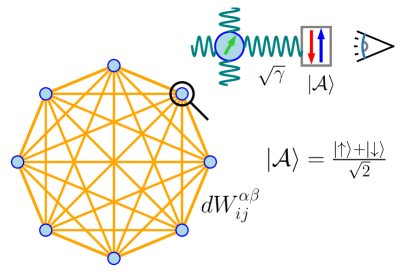
In this letter, we introduce an exactly solvable model of monitored dynamics, composed by a system of $N$ spin-$1/2$ particles with all-to-all pairwise noisy interactions. Each spin is subjected to weak continuous measurements in a random direction. We make use of the aforementioned the replica trick, introducing $n$ identical copies of the system (same noise realisation and same measurement outcomes) and finally considering the $n\to 1$ via analytic continuation. Thanks to the mean-field nature of the interactions, the dynamics is fully encoded in the matrix of overlaps between different replicas which satisfies exact self-consistency equation. Our main result is that the nature of the phase transition depends on $n$: for $n=3$, the system exhibits a first order phase transition, which turns into a second order when $n=2$. More interestingly, we are also able to access the relevant $n\to 1$ limit and we show that the self-consistency equations for the order parameter display logarithmic corrections which stabilise the volume-law phase for arbitrary measurement strength. This implies that the purification time of a mixed state is always exponentially long in the system size. Beyond purification and entanglement, we validate our theory by looking at the full statistics of single-site observables.

The model. —

We consider the Hilbert space $\mathcal{H}=[\mathbb{C}^{2}]^{\otimes N}$ of $N$ spin $1/2$. The spins are continuously monitored in the standard framework of homodyne detection and the stochastic Schrodinger equation [11, 12, 13]. In practice, with a time step $\Delta t$, for each site $i$, we couple each component of the spin $\hat{S}_{i}^{\alpha}$ ($\alpha=x,y,z$) to an auxiliary degree of freedom (ancilla), often chosen to be a single qubit. Subsequently, the ancilla qubit is projectively measured along the $z$ direction with an outcome $a=\pm 1$ . One of the advantages of this approach is that the strength of the system+ancilla coupling can be tuned to have a well-defined $\Delta t\to 0$ limit. Then, the specific details of the discrete-time measurement figure:ocol become irrelevant with the measurement strength parameterised by a unique rate $\gamma$, which we take to be independent from the site $i$ and the direction $\alpha$. The collection of outcomes $\textbf{a}\equiv\{a_{1},\ldots,\}$ defines the signal $M^{\alpha}_{i}(t)=\sqrt{\Delta t}\sum_{n=1}^{t/\Delta t}a_{\tau}$ for each site $i$ and along each direction $\alpha$. Taking into account Born’s rule, in the limit $\Delta t\to 0$, the signal can be shown to obey the stochastic equation [67]

$$dM_{i}^{\alpha}=-2\sqrt{\gamma}\langle\hat{S}_{i}^{\alpha}\rangle+dY_{i}^{\alpha}$$ (1)

where $\langle\hat{S}_{i}^{\alpha}\rangle\equiv\braket{\Psi}{\hat{S}_{i}^{\alpha}}{\Psi}$ and $dY_{i}^{\alpha}$ are centered gaussian white noises, i.e. $\operatorname{\mathbb{E}}[dY_{i}^{\alpha}dY_{i^{\prime}}^{\alpha^{\prime}}]=dt\delta_{i^{\prime}i}^{\alpha^{\prime}\alpha}$ and $\operatorname{\mathbb{E}}[\ldots]$ indicates average over measurement outcomes. Using (1), the evolution of the density matrix due to measurements takes the form (in Ito’s convention)

$$[d\rho]_{\rm meas}=\gamma dt\sum_{i,\alpha}\mathcal{D}_{\hat{S}_{i}^{\alpha}}[\rho]+\sqrt{\gamma}\sum_{i,\alpha}dY_{i}^{\alpha}\{\delta\hat{S}_{i}^{\alpha},\rho\}$$ (2)

where we introduced the dephasing superoperator $\mathcal{D}_{\hat{O}}[\rho]=-\frac{1}{2}[\hat{O},[\hat{O},\rho]]$ and we set $\delta\hat{S}_{i}^{\alpha}=\hat{S}_{i}^{\alpha}-\langle\hat{S}_{i}^{\alpha}\rangle$.

We can now combine the effect of monitoring with the unitary dynamics induced by the interactions between spins. We consider a noisy time-evolution, generated by the Hamiltonian increment

$$d\hat{H}_{0}=\frac{J}{\sqrt{N}}\sum_{1\leq i<j\leq N}\sum_{\alpha,\beta}dW_{ij}^{\alpha\beta}\hat{S}_{i}^{\alpha}\hat{S}_{j}^{\beta}$$ (3)

where $J$ is the coupling strength and $\hat{S}_{i}^{\alpha}$ ($\alpha=x,y,z$) are spin $1/2$ operators acting on the local Hilbert space at site $i$ and $dW_{ij}^{\alpha\beta}$ are also centered Gaussian white noises, with $\operatorname{\mathbb{E}}[dW_{ij}^{\alpha\beta}dW_{i^{\prime}j^{\prime}}^{\alpha^{\prime}\beta^{\prime}}]=dt\delta^{\alpha\beta,\alpha^{\prime}\beta^{\prime}}_{i^{\prime}j^{\prime},ij}$ so the $\operatorname{\mathbb{E}}[\ldots]$ indicates both noise and measurement average. Thus, accounting for Ito’s calculus, the increment of the density matrix due to the unitary dynamics reads

$$[d\rho]_{\rm uni}=-\mathrm{i}[d\hat{H},\rho]+J\sum_{1\leq i<j\leq N}\sum_{\alpha,\beta}\mathcal{D}_{S_{i}^{\alpha}S_{j}^{\beta}}[\rho]\;.$$ (4)

We can combine the two effects in the $\Delta t\to 0$ setting $d\rho=[d\rho]_{\rm uni}+[d\rho]_{\rm meas}$.

For averages of linear quantities in the density matrix $\rho$, e.g. $\operatorname{\mathbb{E}}[\operatorname{tr}[\hat{O}\rho]]$, the dynamics reduces to a Lindblad evolution (although non-trivial behaviors are known already for single-body systems [68, 69, 70]). However, all of them drive the system towards a unique infinite-temperature steady state $\operatorname{\mathbb{E}}[\rho(t\to\infty)]=\mathbf{1}/2^{N}$. The theoretical investigation of nonlinear functionals of $\rho$ is instead much more challenging. In order to avoid this difficulties we make use of the replica trick [60]. Consider, as a nonlinear observable a linear functional in the replica space $\mathcal{O}:\rho\to\operatorname{Tr}^{(k)}[\Omega\rho^{\otimes k}]$ where $\operatorname{Tr}^{(k)}[\ldots]$ is the trace on the extended space $k$-replica space $\mathcal{H}^{\otimes k}$ and $\Omega$ is the Riesz representative of $\mathcal{O}$. An example is the purity defined as $\Pi\equiv\operatorname{tr}[\rho^{2}]=\operatorname{Tr}^{(2)}[\mathbb{S}\rho^{\otimes 2}]$, where the swap operator $\mathbb{S}$ play the role of $\Omega$. Then, the replica trick is based on the identity

$$\mathbb{E}[\mathcal{O}[\rho]]\equiv\mathbb{E}[\operatorname{Tr}^{(k)}[\Omega\rho^{\otimes k}]]=\lim_{n\to 1}\mathbb{E}_{G}[\operatorname{Tr}^{(n)}[\Omega\tilde{\rho}^{\otimes n}_{M}]]$$ (5)

where $\tilde{\rho}_{M}=K_{M}\rho_{0}K_{M}^{\dagger}$ and $K_{M}$ are Kraus operators implementing the unitary and measurement dynamics given the signals $M_{i}^{\alpha}(t)$ [71]. In practice, in order to account for the normalisation and Born’s rule we add $n-k$ replicas assuming $n>k$ and take eventually the $n\to 1$ limit. In the fictitious gaussian average $\mathbb{E}_{G}[\ldots]$, measurement outcomes are unbiased, i.e. the signals are white-noises $\operatorname{\mathbb{E}_{G}}[dM_{i}^{\alpha}dM_{j}^{\beta}]=dt\delta_{ij}\delta^{\alpha\beta}$, as Born’s probability is automatically accounted for in the $n\to 1$ limit. In this case, $\tilde{\rho}$ evolves as $\tilde{\rho}+d\tilde{\rho}=e^{-\mathrm{i}d\hat{H}}\tilde{\rho}e^{\mathrm{i}d\hat{H}^{\dagger}}$, with the non-hermitian Hamiltonian increment given

$$d\hat{H}=d\hat{H}_{0}+\mathrm{i}\sqrt{\gamma}\sum_{\alpha,j}dM_{i}^{\alpha}\hat{S}_{j}^{\alpha}-\frac{\mathrm{i}}{2}\gamma\sum_{j}\hat{S}^{2}_{j}dt\;.$$ (6)

Figure 2: Schematic description of the Keldish path-integral that leads to Eq. (7). After averaging on the unitary noise and the effect of measurements, the replica corresponding to the same contour are coupled by $X^{++}(t)=X^{--}(t)$, while the ones corresponding to different ones by $X^{+-}(t)$. If $\Omega$ does not explicitly break the replica symmetry, the $X$ are time independent, apart from the shadowed transient phase. The operator $\Omega$ acts trivially on $n-k$ replicas.

Replica path integral. —

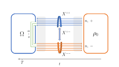
It is useful to express the expectation value in Eq. (5) by means of a Keldysh spin-coherent path integral [72, 73] (see Fig. 2). This amounts to introducing for each site $i=1,\ldots,N$, replica $a=1,\ldots,n$ and Keldysh contour $\sigma=\pm$ a time-dependent classical vector field $\mathbf{s}_{i,a,\sigma}(t)$. Due to the all-to-all nature of the couplings, we have that in the thermodynamic limit the path-integral will be dominated by the saddle-point contributions. This mean we can effectively look at a single-site (replicated) mean-field effective action. As shown in [67], this can be made explicit by performing a Hubbard-Stratonovich transformation [74] and turning back the integral over the $\mathbf{s}_{j,a,\sigma}$ into a single-site evolution. We obtain an action of the form:

$$\mathcal{I}_{n}[X]=\int^{T}_{0}\frac{dt}{2T}\sum_{ab}(X^{+-2}_{ab}-X^{++2}_{ab})-\frac{1}{T}\ln\operatorname{tr}\Bigl{[}\Omega\tilde{\varrho}^{(n)}(T)\Bigr{]},$$ (7)

where the fields $X^{\sigma\sigma^{\prime}}_{ab}(t)$ are conjugated with $\mathbf{s}_{\sigma,a}\cdot\mathbf{s}_{\sigma^{\prime},b}$ (by time reversal, $X^{--}_{ab}$ and $X^{++}_{ab}$ are equal) and $\tilde{\varrho}^{(n)}(T)$ is the effective single-site (unnormalised) density matrix for $n$ replicas, which can be computed by evolving with

$$\begin{split}\frac{d}{dt}\tilde{\varrho}^{(n)}&\equiv\mathcal{L}^{(n)}(\tilde{\varrho}^{(n)})\equiv\sum_{ab}\big{[}(\gamma+X_{ab}^{+-}(t))S^{\alpha}_{a}\tilde{\varrho}^{(n)}S^{\alpha}_{b}\\ &+\frac{1}{2}(\gamma-X_{a,b}^{++}(t))\{\mathbf{S}_{a}\cdot\mathbf{S}_{b},\tilde{\varrho}^{(n)}\}\big{]}-\frac{3}{2}\gamma n\tilde{\varrho}^{(n)}\;.\end{split}$$ (8)

$\mathcal{L}^{(n)}(\tilde{\varrho})$ is the single-site Lindbladian for $n$ replicas.

Saddle-point solution –

We are interested in investigating the saddle-point solutions in order to identify the different phases. The minimization of the functional (7) requires determining the optimal matrices $X_{ab}^{\sigma\sigma^{\prime}}(t)$ for $t\in[0,T]$, which in turns depend on the time-dependent evolution equation (8) and the choice of $\Omega$. However, the action (7) can be seen as a $(0+1)d$ field theory invariant under the action of the group $S_{n}\times S_{n}\times\mathbb{Z}_{2}$, where the two $S_{n}$ represent the permutation group over the $+$ and $-$ replicas respectively, while $\mathbb{Z}_{2}$ exchanges the $+$ with $-$. The simplest assumption, confirmed by numerical checks at $n=2,3$ is that the $\mathbb{Z}_{2}$ remains unbroken, while the $S_{n}$ symmetry between the replicas in the $+$ and $-$ contours to be possibly broken down at large enough $\gamma$. This leads to $n!$ degenerate vacua, in correspondence with permutations $P\in S_{n}$. In order to investigate such a symmetry-breaking transition, we parameterise the solutions in terms of three time-dependent parameters $q(t),r(t),X(t)$

$$\bar{X}^{++}_{ab}=q(t)+\Bigl{(}\frac{3}{4}-q(t)\Bigr{)}\delta_{ab},\;\bar{X}^{+-}_{ab}=r(t)+X(t)\delta_{ab},$$ (9)

where we enforced $X^{++}_{aa}=3/4$ as expected from the normalisation of spin $1/2$. With these choices, $X(t)$ plays the role of a scalar order parameter which tells apart the unbroken ($X=0$) and broken ($X\neq 0$) phases in the identity sector $P=\mathbb{1}$. Using these Ansatzs in Eq. (8), we can project the density matrix onto the eigenspaces with fixed modulus of the total spin $\mathbf{S}_{\rm tot}=\sum_{a}\mathbf{S}_{a}$, labelled by $\mathbf{S}_{\rm tot}^{2}=\ell(\ell+1)$ ($\ell\leq n/2$). Additionally, in the limit of large $T$ and away from the boundaries at $t=0,T$, the fields $q(t),r(t),X(t)$ are expected to attain a bulk $t$-independent value, which will dominate $\mathcal{I}[X]$. This allows us to derive a reduced action only depending on the rescaled order parameter $x=X/(2\gamma+r-q)$, namely

$$\begin{split}\mathcal{I}_{n}(x)=\frac{\left[n(n+x)\left(\frac{3}{4}+2(n-1)\gamma\right)-\Lambda_{n}(x)\right]^{2}}{2n(n-1)(n+2x)}\end{split}$$ (10)

where $\Lambda_{n}(x)$ is the largest eigenvalue of a $\left\lceil{n/2}\right\rceil\times\left\lceil{n/2}\right\rceil$, tridiagonal real and symmetric matrix $L$ whose non-zero elements are given by $L_{\ell,\ell}=(1-\delta_{\ell,0})[\ell(\ell+1)+(n/2+1)x/2]$ and

$$\begin{split}L_{\ell,\ell+1}&=L_{\ell+1,\ell}=\frac{x}{2}\sqrt{\left(\frac{n}{2}-\ell\right)\left(\frac{n}{2}+\ell+2\right)},\end{split}$$ (11)

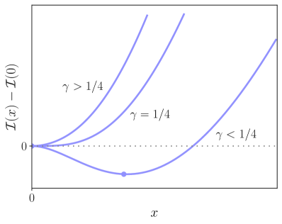
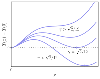
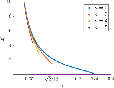
with $\ell=(n\mod 2)/2,\ldots,n/2$. The minimization of $\mathcal{I}_{n}(x)$ leads to the self-consistency equation $\mathcal{I}^{\prime}_{n}(x^{\ast})=0$. We do not know the exact form of $\Lambda_{n}(x)$ for generic $n$ but small values are accessible and instructive. For $n=2$, in agreement with [32], we find an Ising-like second-order transition for $\gamma_{c}=1/4$. Instead, for $n\geq 3$, the transition is discontinuous ($\gamma_{c}=\sqrt{2}/12\approx 0.11$ for $n=3$). This signals that the emergence of a $\mathbb{Z}_{2}$ symmetry in $x$ for $n=2$ is coincidental and not generic. Thus, the relevant $n\to 1$ limit remains undecided. Interestingly, however, such a limit can be accessed exactly, by expanding $\Lambda_{n}(x)$ asymptotically around $x=\infty$, analytically continuing this expression for $n\to 1$, and recognizing a series of the form studied in [75]. As the preservation of the trace ensures that $\mathcal{I}_{n=1}(x)\equiv 0$, we can set $j(x)\equiv\lim_{n\to 1}\mathcal{I}_{n}(x)/(n-1)$ and find (see [67] for details)

$$j(x)=\frac{1}{2(1+2x)}\left[\left(4\gamma+1\right)(1+x)-xk(x)\right]^{2},$$ (12)

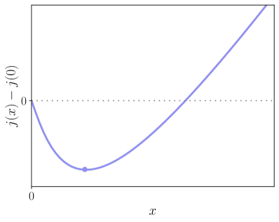
where $k(x)=K_{0}(x)/K_{1}(x)$ and $K_{p}(x)$ denotes the order–$p$ modified Bessel function of the second kind. The function $j(x)$ has only one minimum at a finite $x^{*}(\gamma)>0$, regardless of the value of $\gamma$. By taking the thermodynamic limit first, and then the physical limit $n\rightarrow 1^{+}$ we discover thus that the model does not exhibit any phase transition: rather, the symmetry is broken for every finite $\gamma$ (i.e., $\gamma_{c}=\infty$). This result shows a non-perturbative behavior emerging in the replica limit. Indeed, a Landau-Ginzburg picture should reflect the small–$x$ expansion, $\mathcal{I}_{n}(x)=\mathcal{I}_{n}(0)+\alpha_{n}^{(2)}(\gamma)x^{2}+\alpha_{n}^{(3)}(\gamma)x^{3}+\ldots$, which would naively indicate a second-order phase transition for a vanishing mass term, $\alpha_{n}^{(2)}(\gamma_{c})=0$, consistently with the phenomenology of the $n=2$ case  A generalisation of this approach was employed to derive a finite-dimensional field-theory description in [77, 61]. However, the small–$x$ expansion $j(x)\sim x^{2}\ln(x)$ (up to constants) suggests the non-commutativity of the $x\to 0$ and $n\to 1$ limits. We leave a field-theory justification of this phenomenology to further studies, but we suggest it might result from the degeneracy of the anomalous dimensions of different operators happening at $n\to 1$, a mechanism analogous to the emergence of logarithmic corrections in certain non-unitary conformal field theories [78, 79]. A similar technique can be employed in the forced measurement $n\to 0$, where Born’s probability is discarded and all measurement outcomes are equally weighted [60]. Again, no phase transition appears consistently with the general tendency to weaken measurements decreasing $n$.

Decoupling replicas. —

We now focus on the statistics over trajectories of single-site quantum expectations. Consider for instance the moments $s^{(k)}(T)\equiv\mathbb{E}[\operatorname{Tr}[\rho(T)\hat{S}_{i}^{\alpha}]^{k}]$, where homogeneity and isotropy ensures the independence on the site $i$ and the direction $\alpha$. In our formalism, we can have access to $s^{(k)}$ setting $\Omega=\hat{S}_{i,\alpha}^{\otimes k}$ in Eq. (5). We observe that the boundary condition set by such an $\Omega$ acts non-trivially only on one site and as a consequence, due to an extensive free-energy barrier, cannot change the sector in a symmetry-broken phase. We can thus make direct use of the Ansatz (9) which captures well the identity sector. Nonetheless, while the spectrum of the generalised Lindbladians (8) is sufficient to determine the saddle-point solution in the time bulk $0\ll t\ll T$, it is less suitable for quantitative predictions due to the short/large time transients. An alternative way to proceed is to realise that, once the Ansatz (9) is inserted in (8), we can interpret $\mathcal{L}^{(n)}$ as describing the $n$-replica dynamics of a single spin undergoing noise, measurements and dephasing. We can express the resulting dynamics directly in the $n\to 1$ limit, in the form of the stochastic Schrödinger equation for the single-site normalised density matrix

$$d\varrho=-i\sqrt{\gamma_{2}(t)}dW^{\alpha}[\hat{S}^{\alpha},\varrho]+\sqrt{\gamma_{1}(t)}dM^{\alpha}\{\delta\hat{S}^{\alpha},\varrho\}\\ +\left(\frac{3}{4}+\gamma\right)\mathcal{D}_{S^{\alpha}}[\rho]$$ (13)

where $\delta\hat{S}^{\alpha}=\hat{S}^{\alpha}-\langle\hat{S}^{\alpha}\rangle$, $2\gamma_{1}(t)=2\gamma+3/4-X(t)-q(t)$, $2\gamma_{2}(t)=3/4-X(t)+q(t)$ and and $dW^{\alpha}$, $dM^{\beta}$ are independent Wiener processes ($dW^{\alpha}dW^{\beta}=dM^{\alpha}dM^{\beta}=\delta^{\alpha\beta}dt$) corresponding to unitary and measurement noise respectively.

Figure 3: (a) Behavior of $X(t)$ for $\gamma=0.38$, obtained solving numerically Eq. (13) together with the self-consistency condition (blue), compared with the analytical prediction (gray). (b) Depiction of the stationary distribution $P_{\rm stat}(r)$ of the effective single-replica density operator on the Bloch sphere for $\gamma=0.066$ (orange) and $\gamma=0.38$ (blue) respectively. (c) Histogram of the final distribution (at $t=T$) compared with the stationary one (blue line) at for $\gamma=0.38$.

First of all, the dynamics induced by Eq. (13) can be used to fix self-consistently the parameters $q(t),X(t)$ at all times $t\in[0,T]$. A crucial simplification is obtained by observing that when $\Omega$ is in the identity sector, there is symmetry in the action under $t\to T-t$. Thus, the self-consistency equation for $X(t)$ (and similarly for $q(t)$, see [67]) can be expressed as

$$X(t)=\frac{3}{4}-2E\left(\frac{|\operatorname{tr}[\varrho^{(1)}(t)S^{\alpha}\varrho^{(2)}(T-t)]|^{2}}{\operatorname{tr}[\varrho^{(1)}(t)\varrho^{(2)}(T-t)]}\right)\ .$$ (14)

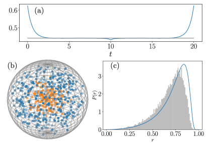
where $\varrho^{(1,2)}$ are two statistically independent solutions of Eq. (13) and $E(\ldots)$ denotes the expectation over the Wiener processes $W^{\alpha},Y^{\beta}$. An accurate solution of (14) can be obtained by introducing the parameterization $\varrho(t)=1/2+r_{\alpha}(t)\hat{S}^{\alpha}$ and exploiting the rotational symmetry leading to a simple stochastic equation for $r(t)=\sqrt{r^{\alpha}(t)r^{\alpha}(t)}$. Numerically solving the resulting stochastic equation and iteratively updating $X(t)$ via (14) quickly leads to a fixed point for all times $t\in[0,T]$, see Fig. 3a. As expected the solution displays a long plateau for $0\ll t\ll T$. In this regime, both $\rho^{(1)}(t)$ and $\rho^{(2)}(T-t)$ in (14) converge in law to a stationary distribution $P_{\rm stat}$, which will in turn determine the bulk (time-independent) value of $X$ via (14). One obtains [67]

$$P_{\rm stat}(r)=\frac{1}{Z}\frac{r^{2}}{(1-r^{2})^{3}}e^{-2x(1-r^{2})^{-1}}$$ (15)

where $Z$ enforces normalization, $r\in(0,1)$ is the modulus of $r^{\alpha}$ and $x=X/(2\gamma_{1})$ is the already-introduced rescaled order parameter. For an eventual unbroken phase ($x=0$) $P_{\rm stat}(r)\to\delta(r-1)$ signaling that $\varrho$ purifies, while for finite $x$ this does not happen, see Fig. 3. As a check it can be verified that the self-consistency equations for $x^{*}(\gamma)$ lead to the same condition $j^{\prime}(x^{*})=0$, with $j(x)$ given by (12) [67]. The agreement between these two approaches substantiates our results beyond the less rigorous aspects of the replica method. Furthermore, with knowledge of $X(t)$ for all $t\in[0,T]$, we obtain $s^{(k)}(T)=E[r_{\alpha}(T)^{k}]=E[r^{k}(T)]/(k+1)$. Note that, because of the behavior around $t\sim T$, the distribution of $r(T\to\infty)$, relevant for single-site observables, differ from $P_{\rm stat}(r)$ describing $r(t)$ in the bulk (see Fig. 3c).

For the calculation of the purity $\Pi(T)$, the operator $\Omega=\mathbb{S}$ simultaneously swaps all sites among $2$ replicas. For this reason, the purification time is an efficient way to detect the existence of a MIPT, as it passes from a value of $O(1)$ (possibly with logarithmic corrections) in the unbroken phase, to an exponentially long value (in $N$), within the broken phase [20, 32]. In the path integral language, this is due to the appearance of an instanton dominating the action, interpolating between different symmetry sectors. The freedom of placing the instanton anywhere in the bulk $0\ll t\ll T$, leads to the estimate $\Pi\sim Te^{-N\mathcal{I}^{*}}$, $\mathcal{I}^{*}$ being the free-energy barrier relative to a single instanton between the identity and the swap sectors in the limit $n\to 1$. The exact calculation of $\mathcal{I}^{*}$ necessitates of an Ansatz for $X^{\sigma\sigma^{\prime}}(t)$ more general than Eq. (9), as it must interpolate between multiple symmetry sectors. Nonetheless, an upper bound for $\mathcal{I}^{*}$ can be obtained assuming an instantaneous jump, so that the instanton can be expressed in terms of the two bulk solution. As shown in [67], this leads to

$$e^{-\mathcal{I}^{*}}\gtrsim 1+(x^{\ast})^{2}-x^{\ast}k(x^{\ast})(x^{\ast}k(x^{\ast})+1).$$ (16)

We expect Eq. (16) to produce a more accurate approximation for $\gamma\to 0$ where $x^{\ast}\sim 3/(8\gamma)$ and $\mathcal{I}^{\ast}\sim 1/2+2\gamma+O(\gamma^{3/2})$. In the opposite limit $\gamma\gg 1$, $x^{\star}$ vanishes exponentially and $\mathcal{I}^{*}\leq\gamma e^{-4\gamma}$: even if it does not vanish, for large $\gamma$ the barrier becomes exponentially small. Such a rapid decay probably makes numerical verification of the absence of a phase transition arduous, since at sufficiently large $\gamma$, to see an exponentially increasing purification time would require reaching sizes $N\gg\mathcal{I}^{\ast}\sim e^{4\gamma}$.

Conclusions. —

We proposed the exact solution of an interacting many-body quantum system subject to continuous isotropic monitoring. Despite the mean-field nature of the solution, we found that the model does not undergo a MIPT: starting from the fully mixed state, the system purifies in a time exponentially long in system size. In terms of the replica formalism, this means that the Landau-Ginzbourg action which describes the system is always in a replica-broken phase. We remark that this is a consequence of the analytic continuation to $n\rightarrow 1$ as, for larger $n$, the system indeed exhibits a spontaneous breaking of the permutational symmetry between replicas corresponding to different Keldysh path in correspondence of a finite $\gamma_{c}$. A natural question is to understand the origin of the logarithmic perturbative corrections appearing in the $n\to 1$ and whether the existence of an area-law / purifying phase could be restored with anisotropic measurements. It is also possible that a $N$-dependent scaling for $\gamma$ could lead to a non-conventional phase transition, similar to what happens in many-body localisation [80] and integrability breaking [81].

Acknowledgements.

We are indebted to Denis Bernard, Pierre Le Doussal, Lorenzo Correale, Chris Baldwin, Jacopo De Nardis, David Huse and in particular Adam Nahum for useful discussions. We thank the Institut Pascal (University of Paris Saclay) and LPTMS for hospitality and support during the ”Dynamical Foundations of Many-Body Quantum Chaos” and ”OpenQMBP2023” programmes. The authors acknowledge support by the ANR JCJC grant ANR-21-CE47-0003 (TamEnt).

Supplementary Material
Elusive phase transition in the replica limit of monitored systems

Appendix A Derivation of the weak measurement equations

A.1 Repeated interaction with the ancilla

Here, we describe briefly how the stochastic Schrödinger equation (SSE) for the weak measurement dynamics can be derived. To simplify the notation, we will consider a generic system evolving under the Hamiltonian $H$ and where a single observable $\hat{O}$ is continuously monitored. First of all, we discretize time considering a finite small interval $\Delta t$. The basic idea is that in a time step $t\in[\tau\Delta t,(\tau+1)\Delta t]$, the system $\mathcal{S}$ is coupled to a (new) ancilla $\mathcal{A}$. For simplicity, the ancilla is supposed to be a spin $1/2$ initial set in the state

$$\ket{\mathcal{A}}=\frac{\ket{+}+\ket{-}}{\sqrt{2}}$$ (SA.1)

At time $t=\tau\Delta t$, the state of the system + ancilla is thus in the factorized state

$$\ket{\Psi_{\tau}}=\ket{\psi_{\tau}}\otimes\ket{\mathcal{A}}$$ (SA.2)

The time evolution up to the next time step $\tau+1$ is performed in two steps:

1. the system and the ancilla evolve unitarily for a time $\Delta t$ and get entangled because of the coupling between them;

2. the $z$-component of the ancilla spin is measured projectively;

Let’s analyse the two steps. Under the unitary evolution $U$, one arrives at

$$\ket{\Psi_{\tau}}^{\prime}=U\ket{\Psi_{\tau}}=(K_{+}\ket{\psi_{\tau}})\otimes\ket{+}+(K_{-}\ket{\psi_{\tau}})\otimes\ket{-}\;,\qquad K_{\pm}=\braket{\pm}{U}{\mathcal{A}}$$ (SA.3)

where we introduced the operators $K_{\pm}$ acting on the Hilbert space of the system $\mathcal{S}$. Unitarity of $U$ and normalization of $\ket{\mathcal{A}}$ imply the only constraint

$$\mathbf{1}_{\mathcal{S}}=\braket{A}{U^{\dagger}U}{A}=K_{+}^{\dagger}K_{+}+K_{-}^{\dagger}K_{-}$$ (SA.4)

where $\mathbf{1}_{\mathcal{S}}$ is the identity operator on the system Hilbert space. This shows that $K_{\pm}$ are Kraus operators.

Measuring the spin $\sigma_{z}$ of the ancilla, one can obtain two possible outcomes $a_{\tau}=\pm 1$. Correspondingly, the state of the system takes the form

$$\ket{\psi_{\tau+1}}=\frac{K_{a_{\tau}}\ket{\psi_{\tau}}}{\sqrt{\braket{\psi_{\tau}}{K_{a_{\tau}}^{\dagger}K_{a_{\tau}}\ket{\psi_{\tau}}}}}$$ (SA.5)

A.2 Scaling limit

We now focus on the scaling limit $\Delta t\to 0$. To do so, we need an explicit form of the operators $K_{\pm}$. For simplicity, we focus on the situation when only one operator $O$ is being monitored, the generalisation being straightforward. Let us first consider the explicit form of the system and ancilla Hamiltonian $\mathcal{S}+\mathcal{A}$. We take

$$U=e^{-\mathrm{i}\Delta tH_{\mathcal{S}+\mathcal{A}}}\;,\quad H_{\mathcal{S}+\mathcal{A}}=H_{0}+\lambda O\sigma_{y}\;.$$ (SA.6)

Choosing $\sigma_{y}$ as the operator on the ancilla is the simplest way to achieve monitoring. The scaling limit is achieved taking $\lambda\to\infty$ and $\Delta t\to 0$ but in such a way that $\gamma=\lambda^{2}\Delta t$ is kept constant where the rate $\gamma$ parameterises the strength of the measurements. With this choice, expanding to the order $O(\Delta t)$, we have

$$U=e^{-\mathrm{i}(\Delta tH_{0}+\sqrt{\gamma\Delta t}O\sigma_{y})}\sim\mathbf{1}-\mathrm{i}\Delta tH_{0}-\mathrm{i}\sqrt{\gamma\Delta t}O\sigma_{y}-\frac{1}{2}\gamma\Delta tO^{2}+O(\Delta t^{3/2})$$ (SA.7)

From the definitions of $K_{\pm}$, we thus obtain

$$K_{\pm}=\frac{1}{\sqrt{2}}\left(\mathbf{1}-\mathrm{i}\Delta tH_{0}\mp\sqrt{\gamma\Delta t}O-\frac{1}{2}\gamma\Delta tO^{2}\right)+O(\Delta t^{3/2})$$ (SA.8)

In order to compute the norm, we expand

$$K_{a}^{\dagger}K_{a}=\frac{1}{2}-a\sqrt{\gamma\Delta t}O+O(\Delta t^{3/2})$$ (SA.9)

Therefore, we have

$$\ket{\psi_{\tau+1}}=\ket{\psi_{\tau}}-\mathrm{i}H_{0}\Delta t\ket{\psi_{\tau}}-a_{\tau}\sqrt{\gamma\Delta t}(O-\langle O\rangle)\ket{\psi_{\tau}}+\frac{3}{2}\gamma\Delta t\langle O\rangle^{2}\ket{\psi_{\tau}}-\gamma\Delta t\langle O\rangle O\ket{\psi_{\tau}}-\frac{1}{2}\gamma\Delta tO^{2}\ket{\psi_{\tau}}+O(\Delta t^{3/2})$$ (SA.10)

where we have introduced the notation $\langle O\rangle=\braket{\Psi_{t}}{O}{\Psi_{t}}$. Finally, to get the continuous time limit as a stochastic differential equation, we observe that the measurement outcome $a_{\tau}$ is a random variable that satisfies

$$\overline{a_{\tau}}=-2\sqrt{\gamma\Delta t}\langle O\rangle\;,\quad\overline{a_{\tau}^{2}}=1\;.$$ (SA.11)

Therefore, defining $M_{\tau}=\sqrt{\Delta t}\sum_{\tau^{\prime}\leq\tau}a_{\tau^{\prime}}$, we find that the variable $Y_{n}$ converges in the limit $\Delta t\to 0$ to a stochastic process solving

$$dM=-2\sqrt{\gamma}\langle O\rangle dt+dM$$ (SA.12)

being $Y_{t}$ a standard Wiener process (i.e. $\overline{dY}=0$ and $\overline{dY^{2}}=dt$). Eq. (SA.12) is easily generalized to Eq. (1) in the main text. Replacing $a_{n}\to dM/\sqrt{\Delta t}$ and using (SA.12) in the limit $\Delta t\to 0$, we recover

$$d\ket{\Psi_{t}}=-\mathrm{i}\hat{H}_{0}dt\ket{\Psi_{t}}+\left(\sqrt{\gamma}[\hat{O}-\langle\hat{O}\rangle_{t}]dY-\frac{\gamma}{2}[\hat{O}-\langle\hat{O}\rangle_{t}]^{2}dt\right)\ket{\Psi_{t}}$$ (SA.13)

This equation can be easily generalised to the case where one simultaneously monitors several observables $O_{1},\ldots$ introducing independent Wiener processes for each operator undergoing monitoring

$$d\ket{\Psi_{t}}=-\mathrm{i}\hat{H}dt\ket{\Psi_{t}}+\sum_{i}\left(\sqrt{\gamma}[\hat{O}_{i}-\langle\hat{O}_{i}\rangle]dY_{i}-\frac{\gamma}{2}[\hat{O}_{i}-\langle\hat{O}_{i}\rangle_{t}]^{2}dt\right)\ket{\Psi_{t}}$$ (SA.14)

From this one can derive the evolution for the density matrix $\rho=\ket{\Psi_{t}}\bra{\Psi_{t}}$

$$d\rho=-\mathrm{i}dt[\hat{H},\varrho]-\gamma\sum_{i}\left[\frac{1}{2}\{\hat{O}_{i}^{2},\varrho\}-O_{i}\varrho O_{i}\right]+\sqrt{\gamma}\sum_{i}dY_{i}\{\hat{O}-\langle\hat{O}\rangle_{t},\varrho\}$$ (SA.15)

A.3 Replica trick

The previous derivation allows computing the average over the outcomes of the measurements of functions on the state $\ket{\Psi_{t}}$. Typical examples are moments of observables:

$$\mathbb{E}(\langle A\rangle^{k})=\int\mathcal{D}YP_{W}(Y)\braket{\Psi_{t}}{A}{\Psi_{t}}^{k}$$ (SA.16)

where $\mathbb{E}(\ldots)$ indicates an averaging over the measurements outcomes, and $P_{W}(Y)$ is the measure over the Wiener processes introduced in Eq. (SA.12). It is also useful to rewrite Eq. (SA.16) in a different way. For simplicity, we go back to the case where only one operator is monitored. Going back to the problem in discretized time and in agreement with Eq. (SA.5), we can write the unnormalized state as

$$\ket{\tilde{\Psi}_{\textbf{a},t}}=K_{a_{N}}\ldots K_{a_{2}}K_{a_{1}}\ket{\Psi_{0}}=\mathcal{K}_{\textbf{a}}\ket{\Psi_{0}}\;,\qquad\mathcal{K}_{\textbf{a}}=K_{a_{N}}\ldots K_{a_{2}}K_{a_{1}}$$ (SA.17)

where the $a_{i}$’s indicate the outcome of the measurements on each ancilla with $N\Delta t=t$. For clarity, we wrote explicitly the dependence on the sequence of measurements as a superscript. Then, we have

$$\mathbb{E}(\langle A\rangle^{k})=\sum_{\textbf{a}}P(\textbf{a})\left(\frac{\braket{\tilde{\Psi}_{\textbf{a},t}}{A}{\tilde{\Psi}_{\textbf{a},t}}}{\braket{\tilde{\Psi}_{\textbf{a},t}}{\tilde{\Psi}_{\textbf{a},t}}}\right)^{k}=\frac{1}{2^{N}}\sum_{\textbf{a}}\braket{\Psi_{0}}{\mathcal{K}^{{\dagger}}_{\textbf{a}}\mathcal{K}_{\textbf{a}}}{\Psi_{0}}^{1-k}\braket{\Psi_{0}}{\mathcal{K}^{{\dagger}}_{\textbf{a}}A\mathcal{K}_{\textbf{a}}}{\Psi_{0}}^{k}$$ (SA.18)

where we used that $P_{\textbf{a}}=\braket{\tilde{\Psi}_{\textbf{a},t}}{\tilde{\Psi}_{\textbf{a},t}}$. Additionally, we can rewrite in the limit of small $\Delta t$

$$K_{a}=\frac{1}{\sqrt{2}}\exp[-i\Delta tH-a\sqrt{\gamma\Delta t}O-\gamma\Delta tO^{2}]+O(\Delta t^{3/2})$$ (SA.19)

Observe that, because of Ito’s calculus, the last term in the exponent must be inserted to obtain the proper expansion up to the order $O(\Delta t)$. We can now take the limit $\Delta t\to 0$. As before, we set $M_{\tau}=\sqrt{\Delta t}\sum_{\tau^{\prime}\leq\tau}a_{\tau^{\prime}}$; however, now the weight $P_{\textbf{a}}$ of the outcome of the measurements has been merged with the expectation value of the observable. As a consequence, the two outcomes $a_{i}=\pm 1$ are equiprobable, and in the limit $\Delta t\to 0$, we recover a unbiased Wiener process, that is $dM^{2}=dt,\mathbb{E}[dM]=0$. Thus, setting in the continuous limit $\mathcal{K}_{t,M}\equiv\lim_{\Delta t\to 0}\mathcal{K}_{\textbf{a}}$, we have

$$\mathbb{E}(\langle A\rangle^{k})=\int\mathcal{D}MP_{W}(M)\braket{\Psi_{0}}{\mathcal{K}^{{\dagger}}_{t,M}\mathcal{K}_{t,M}}{\Psi_{0}}^{1-k}\braket{\Psi_{0}}{\mathcal{K}^{{\dagger}}_{t,M}A\mathcal{K}_{t,M}}{\Psi_{0}}^{k}\;.$$ (SA.20)

Note that in the continuous limit the non-unitary evolution operator $\mathcal{K}_{t,M}$ satisfy

$$\mathcal{K}_{t+dt,M}=e^{-\mathrm{i}d\hat{H}}\mathcal{K}_{t,M}\;,\qquad d\hat{H}=\hat{H}_{0}dt-\mathrm{i}\sqrt{\gamma}dM\hat{O}-\mathrm{i}\gamma\hat{O}^{2}dt$$ (SA.21)

so that $\mathcal{A}$ plays the role of a non-hermitian stochastic Hamiltonian. Its generalisation to many monitored operators leads to Eq. (6) in the main text.

Finally, in order to avoid the presence of a negative exponent $(1-k)$ in the averaging procedure in Eq. (SA.20), we can make use of the replica trick thus replacing $1-k$ with $n-k$. We can define the density matrix for $n$ replicas (SA.21)

$$\rho^{(n)}=\int\mathcal{D}M\underbrace{\tilde{\rho}_{t,M}\otimes\ldots\otimes\tilde{\rho}_{t,M}}_{n}\equiv\mathbb{E}_{G}[\rho_{t,M}^{\otimes n}]\;,\qquad\tilde{\rho}_{t,M}=\mathcal{K}_{t,M}\ket{\Psi_{0}}\bra{\Psi_{0}}\mathcal{K}^{\dagger}_{t,M}\;.$$ (SA.22)

where we introduce the Gaussian expectation $\mathbb{E}_{G}[\ldots]$ where the signal $M$ is treated as a unbiased Wiener process. In this way, we can write via the replica trick

$$\mathbb{E}(\langle A\rangle^{k})=\lim_{n\to 1}\operatorname{Tr}[\rho^{(n)}\underbrace{A\otimes\ldots\otimes A}_{\text{{\hbox{k}} times}}]=\lim_{n\to 1}\operatorname{Tr}[\rho^{(n)}A^{\otimes k}]\equiv\mathbb{E}_{G}[\tilde{\rho}_{M}^{\otimes n}A^{\otimes k}]$$ (SA.23)

which is analogous to Eq. (5) in the main text.

Appendix B Replica path integral

B.1 Derivation of Eqs. (7) and (8) of the main text

We consider the Heisenberg model with disordered Brownian coupling as introduced in the main text. In this section and in the following, we consider a generic value $s$ of the spin for each individual degree of freedom, and eventually we will set $s=1/2$. We want now to derive a path-integral representation for $\mathbb{E}[\mathcal{O}[\rho]]$ in (5). To do so, we exploit the coherent-state path-integral approach. Given the vector $\mathbf{s}=s(\sin\theta\cos\phi,\sin\theta\sin\phi,\cos\theta)$, we introduce the spin-coherent state.

$$\ket{\mathbf{s}(\theta,\phi)}=\prod_{j}e^{-i\mathbf{s}\cdot\mathbf{S}}\ket{\uparrow}_{j}$$ (SB.24)

which leads to the resolution of the identity

$$\frac{2s+1}{4\pi}\int d\omega\ket{\mathbf{s}(\theta,\phi)}\bra{\mathbf{s}(\theta,\phi)}=\mathbf{1}$$ (SB.25)

where $d\omega=s\sin\theta d\theta d\phi$ is a shortcut for the $SU(2)$ measure. We also have

$$\braket{S^{\alpha}}\equiv\bra{\mathbf{s}}S^{\alpha}\ket{\mathbf{s}}=s^{\alpha}$$ (SB.26)

We write the time evolution of the un-normalised density matrix as

$$\rho(t)=e^{-\mathrm{i}d\hat{H}}\ldots e^{-\mathrm{i}d\hat{H}}\rho_{0}e^{\mathrm{i}d\hat{H}^{\dagger}}\ldots e^{-\mathrm{i}d\hat{H}^{\dagger}}\;.$$ (SB.27)

Then, we consider $n$ replicas $\tilde{\varrho}(t)^{\otimes n}$ and introduce a resolution of the identity between each time step, for each spin $i$ and replica $a$. We also use the additional $\pm$ notation to denote the forward/backward time evolution. To avoid some subtleties of Ito’s calculus in the path integral, which are the consequence of the non-smoothness of the Wigner processes $M_{j}^{\alpha}(t)$ and $W_{ij}^{\alpha\beta}(t)$, we consider a regularization procedure. We momentarily assume that the processes $M_{j}^{\alpha}(t)$ and $W_{ij}^{\alpha\beta}(t)$ are smooth and differentiable in time, setting $dM_{j}^{\alpha}=m^{\alpha}_{j}(t)dt$, $dW_{ij}^{\alpha,\beta}=w^{\alpha,\beta}_{ij}(t)dt$. In other words, we have the correlators

$$\mathbb{E}_{G}[w_{ij}^{\alpha\beta}(t)w_{ij}^{\alpha\beta}(t^{\prime})]=\delta_{\epsilon}(t-t^{\prime})\;,\qquad\mathbb{E}_{G}[m_{i}^{\alpha}(t)m_{i}^{\alpha}(t^{\prime})]=\delta_{\epsilon}(t-t^{\prime})$$ (SB.28)

where $\delta_{\epsilon}(t)$ is a smooth mollifier of the Dirac delta while the correlators vanish when any indices are different. Expanding for a short time interval $dt$

$$\begin{split}\bra{\mathbf{s}(t+dt)}&e^{-d\hat{H}}\ket{\mathbf{s}(t)}=\bra{\mathbf{s}(t+dt)}\exp{\left[-i\frac{J}{\sqrt{N}}\sum_{a,i<j}w^{\alpha\beta}_{ij}(t)S^{\alpha}_{i,a}S^{\beta}_{j,a}dt-\sqrt{\gamma}\sum_{a,j}m^{\alpha}_{j}(t)S^{\alpha}_{j,a}dt-\gamma\sum_{a,j}\mathbf{S}_{a,j}^{2}dt\right]}\ket{\mathbf{s}(t)}\\ &=1+\sum_{a}\braket{\delta s}{s_{j,a}}dt-i\frac{J}{\sqrt{N}}\sum_{a,i<j}w^{\alpha\beta}_{ij}(t)\braket{S^{\alpha}_{a,i}S^{\beta}_{a,j}}dt-\sqrt{\gamma}\sum_{a,j}m^{\alpha}_{j}(t)\braket{S^{\alpha}_{a,j}}dt-\gamma nNs(s+1)dt\\ &=\text{exp}\left[\sum_{a}\braket{\delta s}{s_{j,a}}dt-i\frac{J}{\sqrt{N}}\sum_{a,i<j}w^{\alpha\beta}_{ij}(t)s^{\alpha}_{a,i}s^{\beta}_{a,j}dt-\sqrt{\gamma}\sum_{a,j}m^{\alpha}_{j}(t)s^{\alpha}_{a,j}dt-\gamma nNs(s+1)dt\right],\end{split}$$ (SB.29)

where in the last line we implicitly assumed $i\neq j$, as the $i=j$ terms will only result in $O(N^{-1})$ corrections. In the continuum limit we get

$$\mathbb{E}(\mathcal{O})=\overline{\int\mathcal{D}[\mathbf{s}]\ e^{\mathcal{S}[\mathbf{s}]}\ \bra{\mathbf{s}^{-}_{a,j}(T)}\Omega\ket{\mathbf{s}^{+}_{a,j}(T)}\bra{\mathbf{s}^{+}_{a,j}(0)}\varrho_{0}\ket{\mathbf{s}^{-}_{a,j}(0)}},$$ (SB.30)

where $\sigma=\pm$ distinguishes Keldysh contours, $\mathcal{D}[\mathbf{s}]=\prod_{a,j,\sigma}\prod_{t}d\omega_{a,j}^{\sigma}(t)$,

$$\begin{split}\mathcal{S}=\sum^{n}_{a=1}&\sum_{\sigma=\pm}\left[i\sigma\sum_{j}\mathcal{S}_{\rm top}[\mathbf{s}_{j,a\sigma}]-i\frac{J}{\sqrt{N}}\sigma\sum_{i<j}\int dtw_{i,j}^{\alpha\beta}(t)s^{\alpha}_{i,a\sigma}(t)s^{\beta}_{j,a\sigma}(t)-\sqrt{\gamma}\sum_{j}\int m_{j}^{\alpha}(t)s^{\alpha}_{j,a\sigma}(t)\right]\\ &-2\gamma nNTs(s+1),\end{split}$$ (SB.31)

and

$$\mathcal{S}_{\rm top}[\mathbf{s}]=s\int dt\dot{\phi}\left(1-\cos\theta\right)$$ (SB.32)

is the topological term coming from the coherent state overlap. Now we can perform the average over the realizations of both the noises. Taking the $\epsilon\rightarrow 0$ limit we get:

$$\mathbb{E}(\mathcal{O})=\int\mathcal{D}[\mathbf{s}]\ e^{\bar{\mathcal{S}}[\mathbf{s}]}\ \bra{\mathbf{s}^{\sigma}_{a,j}(T)}\Omega\ket{\mathbf{s}^{\sigma}_{a,j}(T)}\bra{\mathbf{s}^{+}_{a,j}(0)}\varrho_{0}\ket{\mathbf{s}^{-}_{a,j}(0)},$$ (SB.33)

where

$$\bar{\mathcal{S}}[\mathbf{s}]=i\sum_{j}\sum_{a,\sigma}\sigma\mathcal{S}_{\rm top}[\mathbf{s}_{a,j,\sigma}]+\frac{\gamma}{2}\sum_{j}\sum_{ab,\sigma\sigma^{\prime}}\int dt\mathbf{s}_{j,a\sigma}\cdot\mathbf{s}_{j,b\sigma^{\prime}}-\frac{J^{2}}{4N}\sum_{ab,\sigma\sigma^{\prime}}\int dt\sigma\sigma^{\prime}\left(\sum_{j}\mathbf{s}_{j,a\sigma}\cdot\mathbf{s}_{j,b\sigma^{\prime}}\right)^{2}.$$ (SB.34)

From now on, we put now $J=1$. Given the all-to-all form of the last interacting term of the right-hand side, it is convenient to exploit the Hubbard-Stratonovich identities

$$e^{A^{2}/4N}\sim\int dXe^{-NX^{2}/4+XA/2}\hskip 28.45274pte^{-A^{2}/4N}=\int dXe^{-NX^{2}/4+iXA/2}$$ (SB.35)

to put it in a more convenient form:

$$\mathbb{E}(\mathcal{O})\sim\int\mathcal{D}[X]e^{-\frac{N}{4}\int dt\sum_{a,b,\sigma,\sigma^{\prime}}(X^{\sigma^{\prime}\sigma}_{a,b})^{2}}\left(\int\mathcal{D}[\mathbf{s}]e^{\mathcal{S}^{\prime}[\mathbf{s}]}\ \bra{\mathbf{s}^{\sigma}_{a,j}(T)}\Omega\ket{\mathbf{s}^{\sigma}_{a,j}(T)}\bra{\mathbf{s}^{+}_{a,j}(0)}\varrho_{0}\ket{\mathbf{s}^{-}_{a,j}(0)}\right)^{N}$$ (SB.36)

where we introduced

$$\mathcal{S}^{\prime}[\mathbf{s}]=\sum_{a,\sigma}i\sigma\mathcal{S}_{\rm top}[\mathbf{s}_{a,\sigma}]+\frac{1}{2}\sum_{ab,\sigma\sigma^{\prime}}\int dt\left(\gamma+\sqrt{-\sigma\sigma^{\prime}}X^{\sigma^{\prime}\sigma}_{a,b}\right)\mathbf{s}_{a\sigma}\cdot\mathbf{s}_{b\sigma^{\prime}}-2\gamma s(s+1)nT$$ (SB.37)

(let us notice that, by construction $X^{+-}_{ab}=X^{-+}_{ba}$). The advantage of this formulation is that now $\mathcal{S}^{\prime}$ acts on each site independently. As long as the observable $\Omega$, and the initial state are invariant under permutation of sites thus we can interpret the term into square brackets as

$$\left(\operatorname{tr}\Omega\varrho(T)\right)^{N}\equiv\int\mathcal{D}[\mathbf{s}]e^{\mathcal{S}^{\prime}[\mathbf{s}]}\ \bra{\mathbf{s}^{\sigma}_{a,j}(T)}\Omega\ket{\mathbf{s}^{\sigma}_{a,j}(T)}\bra{\mathbf{s}^{+}_{a,j}(0)}\varrho_{0}\ket{\mathbf{s}^{-}_{a,j}(0)}$$ (SB.38)

where the single-state $\varrho(t)$ evolves through the equation

$$\begin{split}\frac{d}{dt}\varrho=\sum_{ab}\left[(\gamma+X_{ab}^{+-})s^{\beta}_{a}\varrho s^{\beta}_{b}+\frac{1}{2}(\gamma+iX_{a,b}^{++})(\mathbf{s}_{a}\cdot\mathbf{s}_{b})\varrho+\frac{1}{2}(\gamma+iX_{a,b}^{--})\varrho(\mathbf{s}_{a}\cdot\mathbf{s}_{b})\right]-2\gamma ns(s+1)\varrho.\end{split}$$ (SB.39)

Since our observable now has the form

$$\mathbb{E}(\mathcal{O})\sim e^{NT\left[-\frac{1}{4T}\int dt\sum_{a,b,\sigma,\sigma^{\prime}}(X^{\sigma^{\prime}\sigma}_{a,b})^{2}+\frac{1}{T}\ln\operatorname{tr}(\Omega\tilde{\varrho}(T))\right]},$$ (SB.40)

it is now possible to perform a saddle point expansion in the thermodynamic limit. To do so, it is convenient to analytically continue $X^{\pm\pm}_{a,b}$ to the complex axis. Moreover, because of the exchange symmetry between $+$ and $-$ contours, we can assume $X^{++}_{a,b}=X^{--}_{a,b}$. It follows that the saddle point solution corresponds to the minimization of the effective action

$$\mathcal{I}[X^{+\pm}_{ab}]=\frac{1}{2T}\int dt\sum_{a,b}\left((X^{+-}_{a,b})^{2}-(X^{++}_{a,b})^{2}\right)-\frac{1}{T}\ln\operatorname{tr}\Omega\varrho(T)$$ (SB.41)

where now

$$\begin{split}\frac{d}{dt}\varrho\equiv\mathcal{L}^{(n)}(\varrho)=\sum_{ab}\left[(\gamma+X_{ab}^{+-}(t))S^{\alpha}_{a}\varrho S^{\alpha}_{b}+\frac{1}{2}(\gamma-X_{a,b}^{++}(t))\{\mathbf{S}_{a}\cdot\mathbf{S}_{b},\varrho\}\right]-2\gamma ns(s+1)\varrho.\end{split}$$ (SB.42)

For $s=1/2$, we recover the results of Eq. (7) and Eq. (8) of the main text.

Finally, we notice that, as to to determine $X_{ab}^{+-}(t)$ we have to minimize Eq. (SB.41), we have

$$X^{++}_{aa}=\braket{\mathbf{S}^{2}}=s(s+1)\ .$$ (SB.43)

Appendix C Saddle-point solution

C.1 Derivation of Eq. (10) of the main text

For large time $T$, the effective action will be dominate by the constant bulk value of the $X^{+\pm}_{ab}(t)$ so that we can write

$$\mathcal{I}(X^{+\pm}_{ab})=\frac{1}{2}\sum_{a,b}\left((X^{+-}_{a,b})^{2}-(X^{++}_{a,b})^{2}\right)-\lambda_{n}(X^{+\pm}_{a,b})$$ (SC.44)

where the $X$s are now time-independent quantities, and $\lambda_{n}(X^{+\pm}_{a,b})$ is the maximum eigenvalue of $\mathcal{L}^{(n)}$. Note that using the symmetry of the action, for any permutation $\mathbb{P}$, one can generate different minima by letting $\mathbb{P}$ act on the $+$ replicas (equivalently one could act on the $-$ ones)

$$\begin{split}&X^{+-}_{ab}\left[P\right]\equiv\bar{X}^{+-}_{P(a)b},\\ &X^{++}_{ab}\left[P\right]\equiv\bar{X}^{++}_{P(a)P(b)}\\ &X^{--}_{ab}[P]\equiv\bar{X}^{--}_{a,b}.\end{split}$$ (SC.45)

In the unbroken phase, there will be a unique solution so that all $X^{+\pm}_{ab}$ for all $P$’s coincide, while in the broken phase, this leads to $n!$ solutions. As discussed in the main text, we can assume for the $X^{+\pm}_{ab}$ the ansatz

$$\begin{split}\bar{X}^{+-}_{a,b}&=r+X\delta_{ab}\\ \bar{X}^{++}_{a,b}&=q(1-\delta_{a,b})+s(s+1)\delta_{a,b},\end{split}$$ (SC.46)

where the scalar variable $X$ plays the role of the order parameter. Given that $\varrho_{\rm max}^{\mathbb{1}}$ is the maximum eigenvector of $\mathcal{L}^{(n)}$ in the identity sector, we can obtain the steady states in the other sectors using

$$\varrho_{\rm max}^{\mathbb{P}}\to R[\mathbb{P}^{-1}]\varrho_{\rm max}^{\mathbb{1}}$$ (SC.47)

where $R[\mathbb{P}^{-1}]$ is the representation of the permutation $\mathbb{P}$ in the space of replicas.

In terms of this Eq. (SB.42) becomes

$$\frac{d}{dt}\tilde{\varrho}=(\gamma+r)S^{\alpha}_{\rm tot}\tilde{\varrho}S^{\alpha}_{\rm tot}+\frac{1}{2}(\gamma-q)\{\mathbf{S}^{2}_{\rm top},\tilde{\varrho}\}+X\sum_{a}S^{\alpha}_{a}\tilde{\varrho}S^{\alpha}_{a}+\left(q-2\gamma-s(s+1)\right)ns(s+1)\tilde{\varrho}$$ (SC.48)

where $\mathbf{S}_{\rm tot}=\sum_{a}\mathbf{S}_{a}$. In terms of this parametrization, the effective action $\mathcal{I}$ becomes, up to additive constants,

$$\mathcal{I}(q,r,X)=\left[\frac{1}{2}n(n-1)(r^{2}-q^{2})+\frac{n}{2}(r+X)^{2}-\lambda_{n}(X,q,r)\right]\ .$$ (SC.49)

We can now look for the maximum eigenvector by looking at the replica-symmetric subspace. In turn, this means writing $\tilde{\varrho}$ as linear combination of the projectors $\Pi_{\ell}$ onto the $\mathbf{S}^{2}_{\rm tot}=\ell(\ell+1)$ subspace, with $\ell=n/2-\left\lfloor{n/2}\right\rfloor,\dots,n/2$. The $\Pi_{\ell}$ are normalized as such that $\Pi_{\ell}\Pi_{\ell^{\prime}}=0$ for $\ell\neq\ell^{\prime}$ and $\operatorname{tr}\Pi_{\ell}=1$. Let us note that $S^{\alpha}_{\rm tot}\Pi_{\ell}=\Pi_{\ell}S^{\alpha}_{\rm tot}$ and $\mathbf{S}^{2}_{\rm tot}\Pi_{\ell}=\ell(\ell+1)\Pi_{\ell}$. We thus have that the diagonalization of the operator $\mathcal{L}^{(n)}$ reduces to the diagonalization of the $\left\lceil{n/2}\right\rceil$ by $\left\lceil{n/2}\right\rceil$ matrix

$$\begin{split}(\mathcal{L}^{(n)})_{\ell,\ell^{\prime}}&=\operatorname{tr}\left(\Pi_{\ell^{\prime}}\mathcal{L}^{(n)}(\Pi_{\ell})\right)\\ &=(2\gamma+r-q)\ell(\ell+1)\delta_{\ell,\ell^{\prime}}+X\sum_{a,\alpha}\operatorname{tr}\Pi_{\ell}S_{a}^{\alpha}\Pi_{\ell^{\prime}}S^{\alpha}_{a}+\frac{3}{4}n\left(q-2\gamma-\frac{3}{4}\right)\delta_{\ell,\ell^{\prime}}.\end{split}$$ (SC.50)

As a consequence, we have that

$$\lambda_{n}=(2\gamma+r-q)\Lambda_{n}(x)+s(s+1)n\left(q-2\gamma-s(s+1)\right)$$ (SC.51)

where

$$x=\frac{X}{2\gamma+r-q}$$ (SC.52)

and $\Lambda_{n}(x)$ is the maximum eigenvalue of the matrix

$$L_{\ell,\ell^{\prime}}=\ell(\ell+1)\delta_{\ell,\ell^{\prime}}+x\sum_{a,\alpha}\operatorname{tr}\Pi_{\ell}S_{a}^{\alpha}\Pi_{\ell^{\prime}}S^{\alpha}_{a}\ .$$ (SC.53)

The effective action $\mathcal{I}$,

$$\mathcal{I}=\frac{1}{2}n(n-1)(r^{2}-q^{2})+\frac{n}{2}\left(r+(2\gamma+r-q)x\right)^{2}-(2\gamma+r-q)\Lambda_{n}(x)-s(s+1)nq\ .$$ (SC.54)

is now quadratic in $q$ and $r$ so that the corresponding saddle point equations $\partial_{q}\mathcal{I}=0$, $\partial_{r}\mathcal{I}=0$ can be straighforwardly solved to give an effective action of the $x$ alone, namely

$$\mathcal{I}(x)=\frac{1}{2n(n-1)(n+2x)}\left[n(n+x)\left(s(s+1)+2(n-1)\gamma\right)-\Lambda_{n}(x)\right]^{2},$$ (SC.55)

which, for $s=1/2$, reproduces Eq. (10).

C.2 Derivation of Eq. (11) of the main text

We will now derive the explicit form (11) of the matrix $L$, namely

$$\begin{split}L_{\ell,\ell}&=\ell(\ell+1)+\frac{1}{2}\left(\frac{n}{2}+1\right)x\ \ \forall\ \ell\neq 0\\ L_{\ell,\ell+1}&=L_{\ell+1,\ell}=\frac{x}{2}\sqrt{\left(\frac{n}{2}-\ell\right)\left(\frac{n}{2}+\ell+2\right)},\end{split}$$ (SC.56)

along with $L_{00}=0$ (for $n$ even). Since this expression is only valid for spin-$1/2$, we will now specialize to the case of $s=1/2$. Before proceeding with the derivation let us notice that, since we are now dealing with a collection of spin-$1/2$, we have that the dimension $D_{n,\ell}$ of each eigenspace of $S^{2}_{\rm tot}$ is given by

$$D_{n,\ell}=(2\ell+1)d^{(n)}_{\ell}$$ (SC.57)

where $d^{(n)}_{\ell}$ is the generalized Catalan number

$$d^{(n)}_{\ell}\equiv C_{\ell+n/2,n/2-\ell}=\frac{2\ell+1}{n+1}\begin{pmatrix}n+1\\ n/2-\ell\end{pmatrix}$$ (SC.58)

which account for the degeneracy of the spin-$\ell$ representation.

In order to prove Eq. (SC.56), we have to compute the $x$-proportional term in Eq. (SC.53), which we denote with $B$. We notice that, because of the permutational and rotational invariance:

$$B_{\ell,\ell^{\prime}}\equiv\sum_{a,\alpha}\operatorname{tr}[\Pi_{\ell}S_{a}^{\alpha}\Pi_{\ell^{\prime}}S^{\alpha}_{a}]=3n\operatorname{tr}[\Pi_{\ell}S_{1}^{z}\Pi_{\ell^{\prime}}S^{z}_{1}].$$ (SC.59)

Let us now choose as a basis the tensor product of the single spin $S_{1}^{z}$ and of the sum of the other $n-1$ ones. The Hilbert space corresponding to the latter can be decomposed into a collection of spin-$j$ representations, each of one generated by $\ket{j,m}$, with $m=-j,\ldots,j$. Note that each value of $j$ can be obtained with a degeneracy $d^{(n-1)}_{j}$. It follows that

$$\ket{j,m,\scriptstyle\frac{1}{2}\displaystyle,\scriptstyle\frac{\sigma}{2}\displaystyle}\equiv\ket{j,m,\sigma},$$ (SC.60)

with $\sigma=\pm 1$, constitute a basis for the whole $n$-replica Hilbert space. Since

$$\bra{j^{\prime},m^{\prime},\sigma^{\prime}}S_{1}^{z}\ket{j,m,\sigma}=\frac{\sigma}{2}\delta_{jj^{\prime}}\delta_{mm^{\prime}}\delta_{\sigma\sigma^{\prime}}$$ (SC.61)

and

$$\Pi_{\ell}=\frac{1}{\sqrt{D_{n,\ell}}}\sum_{M=-\ell}^{\ell}\ket{\ell,M}\bra{\ell,M}$$ (SC.62)

we have

$$\begin{split}B_{\ell,\ell^{\prime}}&=\frac{3}{4}\frac{n}{\sqrt{D_{n,\ell}D_{n,\ell^{\prime}}}}\sum_{j,m,m^{\prime},\sigma,\sigma^{\prime}}\sigma\sigma^{\prime}d^{(n-1)}_{j}\bra{j,m,\sigma}\Pi_{\ell}\ket{j,m^{\prime},\sigma^{\prime}}\bra{j,m^{\prime},\sigma^{\prime}}\Pi_{\ell^{\prime}}\ket{j,m,\sigma}\\ &=\frac{3}{4}\frac{n}{\sqrt{D_{n,\ell}D_{n,\ell^{\prime}}}}\sum\sigma\sigma^{\prime}d^{(n-1)}_{j}\braket{j,m,\sigma}{\ell M}\braket{\ell M}{j,m^{\prime},\sigma^{\prime}}\braket{j,m^{\prime},\sigma^{\prime}}{\ell^{\prime}M^{\prime}}\braket{\ell^{\prime}M^{\prime}}{j,m,\sigma}.\end{split}$$ (SC.63)

Of the above Clebsh-Gordan coefficients, the only different from zero are

$$\begin{split}\braket{j=\ell+\scriptstyle\frac{1}{2}\displaystyle,m,\sigma}{\ell M}&=\sqrt{\frac{1}{2}\left(1+\frac{\sigma M}{\ell+1}\right)}\delta_{M,m+\scriptstyle\frac{\sigma}{2}\displaystyle}\\ \braket{j=\ell-\scriptstyle\frac{1}{2}\displaystyle,m,\sigma}{\ell M}&=-\sigma\sqrt{\frac{1}{2}\left(1-\frac{\sigma M}{\ell}\right)}\delta_{M,m+\scriptstyle\frac{\sigma}{2}\displaystyle}.\end{split}$$ (SC.64)

This means that the matrix elements are identically zero if $|\ell-\ell^{\prime}|>1$ and $L$ is tridiagonal. Let us consider the case $\ell^{\prime}=\ell+1$: in this case the only contribution of the sum over $j$ comes from $j=\ell+1/2=\ell^{\prime}-1/2$, i.e.

$$\begin{split}B_{\ell,\ell+1}&=\frac{3}{4}\frac{nd^{(n-1)}_{\ell+\scriptstyle\frac{1}{2}\displaystyle}}{\sqrt{D_{n,\ell}D_{n,\ell+1}}}\sum\sigma\sigma^{\prime}\braket{\ell+\scriptstyle\frac{1}{2}\displaystyle,m,\sigma}{\ell M}\braket{\ell M}{\ell+\scriptstyle\frac{1}{2}\displaystyle,m^{\prime},\sigma^{\prime}}\braket{\ell+\scriptstyle\frac{1}{2}\displaystyle,m^{\prime},\sigma^{\prime}}{\ell+1,M^{\prime}}\braket{\ell+1,M^{\prime}}{\ell+\scriptstyle\frac{1}{2}\displaystyle,m,\sigma}\\ &=\frac{3}{16}\frac{nd^{(n-1)}_{\ell+\scriptstyle\frac{1}{2}\displaystyle}}{\sqrt{D_{n,\ell}D_{n,\ell+1}}}\sum\delta_{M,m+\scriptstyle\frac{\sigma}{2}\displaystyle}\delta_{M^{\prime},m^{\prime}+\scriptstyle\frac{\sigma^{\prime}}{2}\displaystyle}\delta_{M^{\prime}M}\sigma^{2}\sigma^{\prime 2}\sqrt{\left(1+\frac{\sigma M}{\ell+1}\right)\left(1+\frac{\sigma^{\prime}M}{\ell+1}\right)\left(1-\frac{\sigma^{\prime}M^{\prime}}{\ell+1}\right)\left(1-\frac{\sigma M^{\prime}}{\ell+1}\right)}\\ &=\frac{3}{4}\frac{nd^{(n-1)}_{\ell+\scriptstyle\frac{1}{2}\displaystyle}}{\sqrt{D_{n,\ell}D_{n,\ell+1}}}\sum_{M=-\ell}^{\ell}\left(1-\frac{M^{2}}{(\ell+1)^{2}}\right)\\ &=\frac{3}{4}\frac{nd^{(n-1)}_{\ell+\scriptstyle\frac{1}{2}\displaystyle}}{\sqrt{D_{n,\ell}D_{n,\ell+1}}}(2\ell+1)\left(1-\frac{\ell}{3(\ell+1)}\right)\\ &=\frac{n}{4}\frac{d^{(n-1)}_{\ell+\scriptstyle\frac{1}{2}\displaystyle}}{\sqrt{D_{n,\ell}D_{n,\ell+1}}}\frac{(2\ell+1)(2\ell+3)}{\ell+1}\\ &=\frac{1}{2}\sqrt{\left(\frac{n}{2}-\ell\right)\left(\frac{n}{2}+\ell+2\right)}\end{split}$$ (SC.65)

Let us consider now the case $\ell=\ell^{\prime}$: in this case, for $\ell\neq 0$, we have both the contribution $j=\ell-1/2$ and $j=\ell+1/2$

$$\begin{split}B_{\ell,\ell}&=\frac{3}{4D_{n,\ell}}nd^{(n-1)}_{\ell+\scriptstyle\frac{1}{2}\displaystyle}\sum\sigma\sigma^{\prime}\braket{\ell+\scriptstyle\frac{1}{2}\displaystyle,m,\sigma}{\ell M}\braket{\ell M}{\ell+\scriptstyle\frac{1}{2}\displaystyle,m^{\prime},\sigma^{\prime}}\braket{\ell+\scriptstyle\frac{1}{2}\displaystyle,m^{\prime},\sigma^{\prime}}{\ell M^{\prime}}\braket{\ell M^{\prime}}{\ell+\scriptstyle\frac{1}{2}\displaystyle,m,\sigma}\\ &+\frac{3}{4D_{n,\ell}}nd^{(n-1)}_{\ell-\scriptstyle\frac{1}{2}\displaystyle}\sum\sigma\sigma^{\prime}\braket{\ell-\scriptstyle\frac{1}{2}\displaystyle,m,\sigma}{\ell M}\braket{\ell M}{\ell-\scriptstyle\frac{1}{2}\displaystyle,m^{\prime},\sigma^{\prime}}\braket{\ell-\scriptstyle\frac{1}{2}\displaystyle,m^{\prime},\sigma^{\prime}}{\ell M^{\prime}}\braket{\ell M^{\prime}}{\ell-\scriptstyle\frac{1}{2}\displaystyle,m,\sigma}\\ &=\frac{3}{16D_{n,\ell}}nd^{(n-1)}_{\ell+\scriptstyle\frac{1}{2}\displaystyle}\sum\sigma\sigma^{\prime}\delta_{M,m+\scriptstyle\frac{\sigma}{2}\displaystyle}\delta_{M^{\prime},m^{\prime}+\scriptstyle\frac{\sigma^{\prime}}{2}\displaystyle}\delta_{M^{\prime}M}\left(1+\frac{\sigma M}{\ell+1}\right)\left(1+\frac{\sigma^{\prime}M}{\ell+1}\right)\\ &+\frac{3}{16D_{n,\ell}}nd^{(n-1)}_{\ell-\scriptstyle\frac{1}{2}\displaystyle}\sum\sigma\sigma^{\prime}\delta_{M,m+\scriptstyle\frac{\sigma}{2}\displaystyle}\delta_{M^{\prime},m^{\prime}+\scriptstyle\frac{\sigma^{\prime}}{2}\displaystyle}\delta_{M^{\prime}M}\left(1-\frac{\sigma M}{\ell}\right)\left(1-\frac{\sigma^{\prime}M}{\ell}\right)\\ &=\frac{3}{4D_{n,\ell}}nd^{(n-1)}_{\ell+\scriptstyle\frac{1}{2}\displaystyle}\left(\frac{1}{(\ell+1)^{2}}+\frac{1}{\ell^{2}}\right)\sum_{M=-\ell}^{\ell}M^{2}\\ &=\frac{n}{4d^{(n)}_{\ell}}\left(\frac{\ell}{\ell+1}d^{(n-1)}_{\ell+\scriptstyle\frac{1}{2}\displaystyle}+\frac{\ell+1}{\ell}d^{(n-1)}_{\ell-\scriptstyle\frac{1}{2}\displaystyle}\right)\\ &=\frac{1}{2}+\frac{n}{4}.\end{split}$$ (SC.66)

For $\ell=0$ we only have the $\ell=1/2$ contribution, so that

$$B_{00}=0.$$ (SC.67)

Figure S1: Sketch of the Landau-Ginzburg action $\mathcal{I}(x)$ for $n=2$ (left) and $n=3$ (right). While for $n=2$ we have a second order phase transition, for $n=3$ we have a finite jump.

C.3 Integer number of replicas $n>1$

Case: $n=2$

We have $\ell=1,0$ and

$$L=\begin{pmatrix}2&0\\ 0&0\end{pmatrix}+x\begin{pmatrix}1&\sqrt{3}/2\\ \sqrt{3}/2&0\end{pmatrix}.$$ (SC.68)

As a consequence

$$\Lambda_{2}(x)=1+\frac{x}{2}+\sqrt{1+x+x^{2}},$$ (SC.69)

and finally

$$\mathcal{I}_{2}(x)=\frac{2}{1+x}\left[\left(\gamma+\frac{1}{4}\right)(2+x)-\frac{1}{4}\sqrt{1+x+x^{2}}\right]^{2}.$$ (SC.70)

Even if this function is not even in $x$, we have

$$\mathcal{I}_{2}(x)=2\left(\gamma+\frac{1}{8}\right)\left(\gamma-\frac{1}{4}\right)(x^{2}-x^{3})+O(x^{4})$$ (SC.71)

so that for $\gamma=1/4$ both the second and the third order vanish. As a consequence we find an Ising-like transition between a broken phase ($\gamma<\gamma_{c}\equiv 1/4$) and the $x=0$ phase ($\gamma>\gamma_{c}$) in which the permutational symmetry is restored (see Fig. S1, left panel). This result is consistent with [32], in which the approximation $n=2$ is implicitly assumed.

Case: $n=3$

We have $\ell=3/2,1/2$ and

$$L=\begin{pmatrix}15/4&0\\ 0&3/4\end{pmatrix}+x\begin{pmatrix}5/4&1\\ 1&5/4\end{pmatrix}\;.$$ (SC.72)

As a consequence

$$\Lambda_{3}(x)=\frac{9}{4}+\frac{5}{4}x+\frac{1}{2}\sqrt{9+4x^{2}},$$ (SC.73)

and finally

$$\mathcal{I}_{3}(x)=\frac{12}{3+2x}\left[\left(\gamma+\frac{1}{12}\right)(x+3)+\frac{1}{8}-\frac{1}{8}\sqrt{1+\frac{4}{9}x^{2}}\right]^{2}.$$ (SC.74)

$\mathcal{I}_{3}(x)$ has a minimum in $x=0$ for every $\gamma>1/12\approx 0.083$, and another one, corresponding to a finite $x$, for any $\gamma<1/24(1+7/\sqrt{13})\approx 0.123$. The two minima become degenerate for $\gamma=\gamma_{c}=\sqrt{2}/12\approx 0.118$ (corresponding to $x=0$, $x=3/2$), signaling the presence of a discontinuous transition from $x=3/2$ to $x=0$ at $\gamma=\gamma_{c}$ (see Fig. S1, right panel).

Case: $n>3$

For $n>3$ the expression for $\Lambda(x)$ is no longer treatable analytically, so that it is not possible to derive the explicit value of $\gamma_{c}$. The numerical analysis, however, suggest a scenario similar to the one for $n=3$, so that the phase transition is expected to be discontinuous for any $n\geq 3$ (see Fig. S2 left panel).

Figure S2: Left: Behavior of the minimum $x^{*}$ of the Landau-Ginzburg action $\mathcal{I}(x)$ for $n=2$ to $n=5$. While for any $n$ $x^{*}\equiv 0$ for any $\gamma>\gamma_{c}$, $x^{*}(\gamma)$ is continuous only for $n=0$. Right: Sketch of the Landau-Ginzburg action $\mathcal{I}(x)$ for $n\rightarrow 1^{+}$: regardless of the value of $\gamma$ we have a minimum in correspondence of a finite $x$, signaling that $\gamma_{c}\rightarrow\infty$ as $n\rightarrow 1^{+}$.

C.4 The $n\rightarrow 1$ replica limit

As we do not have the generic analytic form of $\Lambda_{n}(x)$, it is not straightforward to take the $n\rightarrow 1$ limit. As $\Lambda_{n}(0)=n(n+2)/4$, a perturbative expansion around $x=0$ could be carried out; unfortunately, the higher order ($\geq 3$) coefficients of these expansions turn out to be non-analytic functions of $n$. On the other hand, we can notice that the matrix $B=\partial_{x}L$ introduced in Eq. (SC.59) can be expressed in terms of $SU(2)$ ladder operators, so that its spectrum $\{b_{p}\}$ is given by

$$b_{p}=\frac{3}{4}n-2p$$ (SC.75)

with $p=0,\cdots,\left\lceil{n/2}\right\rceil$. Therefore, $\Lambda_{n}(x)\sim 3n/4x$ for $x\gg 1$, and it is possible to carry out a perturbative expansion around $x=\infty$ obtaining

$$\Lambda_{n}(x)=\frac{3}{4}n(1+x)+n(n-1)\sum^{\infty}_{k=1}P_{k}(n)x^{-k}$$ (SC.76)

where $P_{k}(n)$ are increasingly complicated degree $k-1$ polynomials in $n$. In the vicinity of $n=1$ we get

$$\Lambda_{n}(x)=\frac{3}{4}n(1+x)+(n-1)\left(\frac{3}{16}\frac{1}{x}-\frac{3}{16}\frac{1}{x^{2}}+\frac{63}{256}\frac{1}{x^{3}}-\frac{27}{64}\frac{1}{x^{4}}+\frac{1899}{2048}\frac{1}{x^{5}}-\frac{81}{32}\frac{1}{x^{6}}+\cdots\right)+O(n-1)^{2}.$$ (SC.77)

Even if it is not straightforward to determine the analytic dependency on $n$ of the generic term of this asymptotic expansion, one can recognize in the square bracket term the expansion of

$$\frac{K_{0}(x)}{K_{1}(x)}=1-\frac{1}{2x}+\frac{3}{8}\frac{1}{x^{2}}-\frac{3}{8}\frac{1}{x^{3}}+\frac{63}{128}\frac{1}{x^{4}}-\frac{27}{32}\frac{1}{x^{5}}+\frac{1899}{1024}\frac{1}{x^{6}}-\frac{81}{16}\frac{1}{x^{7}}+\cdots\$$ (SC.78)

where $K_{p}(x)$ denotes the order-$p$ modified Bessel function of the second kind (see [75] for an analysis of this series). We have the following

$$\Lambda_{n}(x)=\frac{3}{4}(1+x)+(n-1)\left(1+\frac{x}{4}+\frac{x}{2}\frac{K_{0}(x)}{K_{1}(x)}\right)+O(n-1)^{2}.$$ (SC.79)

Finally, we find

$$\mathcal{I}(x)=\frac{2(n-1)}{1+2x}\left[\left(\gamma+\frac{1}{4}\right)(1+x)-\frac{x}{4}\frac{K_{0}(x)}{K_{1}(x)}\right]^{2}+O(n-1)^{2}.$$ (SC.80)

As expected the action vanishes for $n=1$, so we inspect the behavior for $n\to 1$. As it happens often in replica limits of disordered systems, the nature of minima/maxima in the Landau-Ginzburg action changes for $n\to 1^{+}$ and $n\to 1^{-}$. It is clear that the physical limit for us corresponds to $n\rightarrow 1^{+}$, regardless of the value of $\gamma$, as for $n<1$, the action is not bounded from below. For $n\to 1^{+}$, the action always has a local maximum for $x=0$ ($\mathcal{I}(x)\sim\mathcal{I}(0)+x^{2}\ln x$) and a minimum for finite $x$ (see Fig. S2, right panel). So, as stated in the main text, the system is always in the broken phase, that is, $x^{\ast}>0$ for any $\gamma$. Small and large $x$ expansions of Eq. (SC.80) give the asymptotic regimes

$$x^{\ast}\sim\frac{3}{8\gamma}\to\infty\;,\qquad\gamma\to 0$$ (SC.81)

$$x^{\ast}\sim 2e^{-2\gamma-\gamma_{\rm EM}-1}\;,\qquad\gamma\to\infty$$ (SC.82)

where $\gamma_{\rm EM}$ is the Euler-Mascheroni constant.

C.5 The $n\rightarrow 0$ replica limit

To compute the $n\rightarrow 0$, we can start again from Eq. (SC.76). In this case, we get:

$$\Lambda_{n}(x)=n\left(\frac{3}{4}-\frac{3}{16}\frac{1}{x}+\frac{9}{32}\frac{1}{x^{2}}-\frac{153}{256}\frac{1}{x^{3}}+\frac{819}{512}\frac{1}{x^{4}}-\frac{10449}{2048}\frac{1}{x^{5}}+\frac{76977}{4096}\frac{1}{x^{6}}\dots\right)+O(n^{2})$$ (SC.83)

in which we can recognize the asymptotic expansion of

$$\Lambda_{n}(x)=\frac{n}{2}\left(\frac{K_{1}(x)}{K_{1}(x)-K_{0}(x)}-2x\right)+O(n^{2})\ .$$ (SC.84)

Injecting this result in the action, we have:

$$\mathcal{I}(x)=-\frac{n}{x}\left[\left(\gamma-\frac{7}{8}\right)x-\frac{1}{4}\frac{K_{1}(x)}{K_{1}(x)-K_{0}(x)}\right]^{2}+O(n^{2})\ .$$ (SC.85)

In this case the only physical choice is to send $n\rightarrow 0^{-}$ as, in the other case, $\mathcal{I}(x)$ is not bounded from below. Once again, we get the broken solution $x=x^{*}(\gamma)\neq 0$ for every value of $\gamma$. At large $\gamma$, $x^{\ast}=\sqrt{3/(16\gamma}+O(\gamma^{-3/4}\to 0$ as expected. Nonetheless, $\gamma<11/8$, $x^{\ast}$ grows with $\gamma$ and interestingly $x^{\ast}(\gamma)\to\infty$ for $\gamma\to 11/8$. We leave the study of the behavior at small $\gamma$ of the $n\to 0$ for future studies.

Appendix D Decoupling of replicas

D.1 Derivation of Eq. (13) of the main text

Now we want to derive the evolution equation (13) for $\tilde{\varrho}$, and the corresponding self-consistent condition on the components of $X^{+\pm}$. In this paragraph we show how the $n\rightarrow 1$ limit can be obtained directly from Eq. (8) of the main text, which gives the evolution of $\tilde{\varrho}(t)$, once the ansatz (SC.46) has been taken into account. In particular, it is convenient to resort to the path-integral representation of the evolution of $\tilde{\varrho}(t)$, which follows immediately from Eq. (SB.38), namely

$$\operatorname{tr}\Omega\tilde{\varrho}(T)=\int\mathcal{D}[\mathbf{s}]e^{\mathcal{S}^{\prime}}\ \bra{\mathbf{s}^{\sigma}_{a}(T)}\Omega\ket{\mathbf{s}^{\sigma}_{a}(T)}\bra{\mathbf{s}^{+}_{a}(0)}\tilde{\varrho}_{0}\ket{\mathbf{s}^{-}_{a}(0)}.$$ (SD.86)

where $\mathcal{S}^{\prime}$ is given by Eq. (SB.37)

$$\mathcal{S}^{\prime}=\sum_{a,\sigma}i\sigma\mathcal{S}_{\rm top}[\mathbf{s}_{a,\sigma}]+\frac{1}{2}\sum_{ab}\int dt\left((\gamma-X^{++}_{a,b})(\mathbf{s}_{a+}\cdot\mathbf{s}_{b+}+\mathbf{s}_{a-}\cdot\mathbf{s}_{b-})+2(\gamma+X^{+-}_{a,b})\mathbf{s}_{a+}\cdot\mathbf{s}_{b-}\right)-\frac{3}{2}\gamma nT\ ,$$ (SD.87)

where the analytic continuation of $X^{++}$ has been taken into account. Now, by replacing the form of ansatz (SC.46) we get

$$\begin{split}\mathcal{S}^{\prime}&=\sum_{a,\sigma}i\sigma\mathcal{S}_{\rm top}[\mathbf{s}_{a,\sigma}]+\frac{1}{2}\sum_{ab}\int dt\left((\gamma-q)(\mathbf{s}_{a+}\cdot\mathbf{s}_{b+}+\mathbf{s}_{a-}\cdot\mathbf{s}_{b-})+2(\gamma+r)\mathbf{s}_{a+}\cdot\mathbf{s}_{b-}\right)\\ &+\frac{1}{2}\sum_{a}\int dt\left((q-3/4)(\mathbf{s}_{a+}^{2}+\mathbf{s}_{a-}^{2})+2X\mathbf{s}_{a+}\cdot\mathbf{s}_{b-}\right)-\frac{3}{2}\gamma nT\\ &=\sum_{a,\sigma}i\sigma\mathcal{S}_{\rm top}[\mathbf{s}_{a,\sigma}]+\frac{\gamma-q}{2}\int dt\left[\left(\sum_{a}\mathbf{s}_{a+}\right)^{2}+\left(\sum_{a}\mathbf{s}_{a-}\right)^{2}\right]+(\gamma+r)\int dt\left(\sum_{a}\mathbf{s}_{a+}\right)\cdot\left(\sum_{b}\mathbf{s}_{b-}\right)\\ &+X\sum_{a}\int dt\ \mathbf{s}_{a+}\cdot\mathbf{s}_{a-}+\frac{3}{4}\left(q-\frac{3}{4}-2\gamma\right)nT\\ &=\sum_{a,\sigma}i\sigma\mathcal{S}_{\rm top}[\mathbf{s}_{a,\sigma}]+\frac{2\gamma+r-q}{4}\int dt\left(\sum_{a,\sigma}\mathbf{s}_{a\sigma}\right)^{2}-\frac{r+q}{4}\int dt\left(\sum_{a,\sigma}\sigma\mathbf{s}_{a\sigma}\right)^{2}\\ &+X\sum_{a}\int dt\ \mathbf{s}_{a+}\cdot\mathbf{s}_{a-}+\frac{3}{4}\left(q-\frac{3}{4}-2\gamma\right)nT\ .\end{split}$$ (SD.88)

Now we can apply once again the Hubbard-Stratonovich identites

$$e^{A^{2}/4}\sim\int dhe^{-h^{2}+hA}\hskip 28.45274pte^{-A^{2}/4}=\int dhe^{-h^{2}+ihA}$$ (SD.89)

to decouple the different replicas and write

$$\operatorname{tr}\Omega\tilde{\varrho}(T)=\int\mathcal{D}[\mathbf{h}]e^{-\frac{1}{2}\int dt\left[\mathbf{h_{1}}^{2}/\gamma_{1}+\mathbf{h_{2}}^{2}/\gamma_{2}\right]}\int\mathcal{D}[\mathbf{s}]e^{\sum_{a}\tilde{\mathcal{S}}[\mathbf{s}_{a,\sigma}]}\ \bra{\mathbf{s}^{\sigma}_{a}(T)}\Omega\ket{\mathbf{s}^{\sigma}_{a}(T)}\bra{\mathbf{s}^{+}_{a}(0)}\tilde{\varrho}_{0}\ket{\mathbf{s}^{-}_{a}(0)}.$$ (SD.90)

where

$$\gamma_{1}=\gamma+\frac{1}{2}(r-q)\hskip 28.45274pt\gamma_{2}=\frac{1}{2}(r+q)\$$ (SD.91)

and

$$\tilde{S}[\mathbf{s}_{a,\sigma}]=\sum_{\sigma}\int dt\left(i\sigma\mathcal{S}_{\rm top}[\mathbf{s}_{a,\sigma}]+(\mathbf{h}_{1}+i\sigma\mathbf{h}_{2})\cdot\mathbf{s}_{a,\sigma}\right)+X\int dt\ \mathbf{s}_{a,+}\cdot\mathbf{s}_{a,-}+\frac{3}{4}\left(q-\frac{3}{4}-2\gamma\right)T.$$ (SD.92)

To proceed further, it is useful to realise that Eq. (SD.92) could be seen as the path-integral representation for the time evolution of the unnormalised density matrix $\tilde{\varrho}$ of a single spin

$$\tilde{\varrho}+d\tilde{\varrho}=e^{-id\mathscr{H}}\tilde{\varrho}e^{id\mathscr{H}^{\dagger}}+X\sum_{\alpha}\mathcal{D}_{S^{\alpha}}[\tilde{\varrho}]\;,\qquad d\mathscr{H}=(\sqrt{\gamma_{1}}dW^{\alpha}+i\sqrt{\gamma_{2}}dM^{\alpha})S^{\alpha}dt$$ (SD.93)

where additive constants have been ignored as they cancel in the final replica limit and we introduced standard and independent Wiener processes $\sqrt{\gamma_{1}}dW^{\alpha}\sim h_{1}^{\alpha}dt$ and $\sqrt{\gamma_{2}}dM^{\alpha}\sim h_{2}^{\alpha}dt$. Comparing with (SA.21), we see that in the replica limit $n\to 1$, the evolution of $\tilde{\varrho}$ corresponds to a single-spin undergoing noisy unitary dynamics, monitoring and dephasing. We can thus recast the time-evolution already accounting for the normalisation and the Born’s weight over trajectories, using the standard form of the quantum state diffusion

$$d\varrho=\left(\frac{3}{4}+\gamma\right)\left(S^{\alpha}\varrho S^{\alpha}-\frac{3}{4}\varrho\right)+\sqrt{\gamma_{1}}dY^{\alpha}\{S^{\alpha}-\braket{S}^{\alpha},\varrho\}-i\sqrt{\gamma_{2}}dW^{\alpha}[S^{\alpha},\varrho]\ .$$ (SD.94)

Then, from the solutions of Eq. (SD.93) and (SD.94), we introduce noise-dependent time evolution operators such that

$$\tilde{\varrho}_{t_{2}}=\tilde{\mathcal{U}}_{t_{1},t_{2}}^{(\mathbf{W},\mathbf{M})}[\tilde{\varrho}_{t_{1}}]\;,\qquad\varrho_{t_{2}}=\mathcal{U}_{t_{1},t_{2}}^{(\mathbf{W},\mathbf{Y})}[\varrho_{t_{1}}]\;.$$ (SD.95)

In this way, we have the equality for any $k$-replica operator $\Omega$

$$E_{\mathbf{W},\mathbf{M}}(\operatorname{tr}(\Omega\tilde{\varrho}^{\otimes k}_{t})\operatorname{tr}(\tilde{\varrho})^{1-k})=E_{\mathbf{W},\mathbf{Y}}(\operatorname{tr}(\Omega\varrho^{\otimes k}_{t}))$$ (SD.96)

where we used $X+r=3/4$, required for the conservation of the trace. One can verify that it matches with Eq. (13) in the main text. For clarity we stress that the Wiener processes $M^{\alpha}$ and $W^{\alpha}$ are effective single-site noises emerging at the mean-field level and are not directly related with those appearing in Eqs. (2, 3). Via the parameters $\gamma_{1},\gamma_{2}$, the time evolution (SD.94) depends on $q$ and $r$, which are time-dependent quantities to be fixed through the saddle-point equations. To proceed further, we focus on the case where $\Omega=\mathbb{1}$, which is relevant for the calculation of the moments of few-body observables. Usig that $X_{ab}^{++}=q$ and $X_{ab}^{+-}=r$ for $a\neq b$, we have

$$\begin{split}&q(t)=E_{\mathbf{W},\mathbf{M}}\left(\frac{\operatorname{tr}\left(\ \tilde{\mathcal{U}}_{[t,T]}\bigl{[}S^{\alpha}\tilde{\mathcal{U}}_{[0,t]}[\tilde{\varrho}_{0}]\bigr{]}\right)\operatorname{tr}\left(\ \tilde{\mathcal{U}}_{[t,T]}\bigl{[}S^{\alpha}\tilde{\mathcal{U}}_{[0,t]}[\tilde{\varrho}_{0}]\bigr{]}\right)}{\operatorname{tr}\left(\ \tilde{\mathcal{U}}_{[0,T]}[\tilde{\varrho}_{0}]\right)}\right)\\ &r(t)=\frac{3}{4}-X(t)=E_{\mathbf{W},\mathbf{M}}\left(\frac{\operatorname{tr}\left(\ \tilde{\mathcal{U}}_{[t,T]}\bigl{[}S^{\alpha}\tilde{\mathcal{U}}_{[0,t]}[\tilde{\varrho}_{0}]\bigr{]}\right)\operatorname{tr}\left(\ \tilde{\mathcal{U}}_{[t,T]}\bigl{[}\tilde{\mathcal{U}}_{[0,t]}[\tilde{\varrho}_{0}]\bigr{]}S^{\alpha}\right)}{\operatorname{tr}\left(\ \tilde{\mathcal{U}}_{[0,T]}[\tilde{\varrho}_{0}]\right)}\right)\ \end{split}$$ (SD.97)

To write down explicitly the saddle-point equations directly in terms of (SD.94), we could make use of Eq. (SD.96), however the insertion of the operators $S^{\alpha}_{a}$ at a time $t\in[0,T]$ requires a slightly different approach. We use that the evolutions $\tilde{\mathcal{U}}_{[0,t]}$ and $\tilde{\mathcal{U}}_{[t,T]}$ are uncorrelated and the time-reversal symmetry ensuring $q(t)=q(T-t),r(t)=r(T-t),X(t)=X(T-t)$. We denote as $\tilde{\varrho}_{t}^{(1)}=\tilde{\mathcal{U}}_{[0,t]}(\tilde{\varrho}_{0})$ and $2\tilde{\varrho}_{T-t}^{(2)}=\tilde{\mathcal{U}}_{[0,t]}(\mathbb{1})$ and use that $\operatorname{tr}\left(\ \tilde{\mathcal{U}}_{[0,T]}[\tilde{\varrho}_{0}]\right)=\operatorname{tr}\left(\ \tilde{\mathcal{U}}_{[t,T]}\tilde{\mathcal{U}}_{[0,t]}[\tilde{\varrho}_{0}]\right)=2\operatorname{tr}(\tilde{\varrho}_{T-t}^{(2)}\tilde{\varrho}_{t}^{(1)})$, to write

$$q(t)=E_{\mathbf{W},\mathbf{M}}\left(\frac{2\operatorname{tr}\left(\tilde{\varrho}_{T-t}^{(2)}S^{\alpha}\tilde{\varrho}_{t}^{(1)}\right)\times\operatorname{tr}\left(\tilde{\varrho}_{T-t}^{(2)}S^{\alpha}\tilde{\varrho}_{t}^{(1)}\right)}{\operatorname{tr}(\tilde{\varrho}_{T-t}^{(2)}\tilde{\varrho}_{t}^{(1)})}\right)=2E\left(\frac{\operatorname{tr}[\varrho^{(1)}_{t}S^{\alpha}\varrho^{(2)}_{T-t}]\operatorname{tr}[\varrho^{(1)}_{t}S^{\alpha}\varrho^{(2)}_{T-t}]}{\operatorname{tr}[\varrho^{(1)}_{t}\varrho^{(2)}_{T-t}]}\right)_{\varrho^{(1)},\varrho^{(2)}}$$ (SD.98)

where the average are taken over the stochastic variables $\varrho^{(1)}(t)$, $\varrho^{(2)}(T-t)$ which correspond to two independent evolution of the initial single-site density matrix $\varrho=\mathbb{1}/2$ with Eq. (SD.94) at times $t$ and $T-t$ respectively. Similarly, for

$$\frac{3}{4}-X(t)=2E\left(\frac{\operatorname{tr}[\varrho^{(1)}_{t}S^{\alpha}\varrho^{(2)}_{T-t}]\operatorname{tr}[\varrho^{(2)}_{T-t}S^{\alpha}\varrho^{(1)}_{t}]}{\operatorname{tr}[\varrho^{(1)}_{t}\varrho^{(2)}_{T-t}]}\right)_{\varrho^{(1)},\varrho^{(2)}}\ ,$$ (SD.99)

D.2 Derivation of Eq. (15) of the main text

In the limit $T\to\infty$ and for $0\ll t\ll T$, the values of the parameters $X(t)$ and $q(t)$ reach a plateau, and both $\varrho^{(1)}(t)$ and $\varrho^{(2)}(T-t)$ are drawn from the same stationary distribution. We derive now the explicit form of this stationary distribution, given in (15) in the main text. Let us parameterise the state of the single spin as

$$\varrho=\frac{1}{2}+r_{\alpha}S^{\alpha}\;,\qquad\operatorname{tr}(\varrho S^{\alpha})=\frac{1}{2}r_{\alpha}\ ,$$ (SD.100)

in terms of a vector $r^{\alpha}$. Positivity requires $r=\sqrt{r_{\alpha}r_{\alpha}}=\sqrt{R}\leq 1$ and the state is pure for $r=1$. Plugging this into Eq.,(SD.94), we obtain stochastic equations for $r_{\alpha}$

$$dr_{\alpha}=2\operatorname{tr}[d\varrho S^{\alpha}]=-\sqrt{\gamma_{2}}\epsilon_{\alpha\beta\gamma}dW^{\beta}r_{\gamma}+\sqrt{\gamma_{1}}dY^{\alpha}-\sqrt{\gamma_{1}}r_{\alpha}dY^{\beta}r_{\beta}-(\gamma+3/4)r_{\alpha}dt\;.$$ (SD.101)

Analysing this equation, it is clear that it describes the motion of a vector $r_{\alpha}$, whose angular part diffuses isotropically. Instead, for its squared length $R=r_{\alpha}r_{\alpha}$, we obtain after some manipulations

$$dR=2\sqrt{\gamma_{1}}(R^{1/2}-R^{3/2})dB+\gamma_{1}\left(R^{2}-4R+3\right)dt-2XRdt\ .$$ (SD.102)

where we introduced $dY^{\alpha}r_{\alpha}=\sqrt{r_{\alpha}r_{\alpha}}dB=\sqrt{R}dB$, with $dB$ a single Wiener Process with $dB^{2}=dt$ (Wiener processes can be summed in quadrature). Finally, in terms of $r=\sqrt{R}$

$$dr=dt\left(\frac{\gamma_{1}}{r}-r(\gamma_{1}+X)\right)+\sqrt{\gamma_{1}}dB\left(1-r^{2}\right)$$ (SD.103)

To find the stationary distribution, it is useful to make a change of variable and recast this equation in the Langevin form. We set

$$[0,\infty)\ni\omega=\operatorname{arctanh}(r)\;,\qquad r=\tanh(\omega)\in[0,1)\ ,$$ (SD.104)

so that the new variable $\omega$ satisfies the Langevin equation

$$d\omega=\sqrt{\gamma_{1}}dB-dtV^{\prime}(\omega)$$ (SD.105)

with the potential

$$V(\omega)=\frac{1}{2}X\cosh^{2}(\omega)-\gamma_{1}\log(\sinh(2\omega))\ .$$ (SD.106)

We can thus directly write down the stationary distribution

$$P_{\rm stat}(\omega)=\frac{1}{Z}e^{-2V(\omega)/\gamma_{1}}=\frac{1}{Z}\sinh^{2}(2\omega)e^{-2x\cosh^{2}(\omega)}\ ,$$ (SD.107)

where we used the fact that that $x=X/(2\gamma_{1})$. Equivalently, in termsof the variable $r$

$$P_{\rm stat}(r)=P_{\rm stat}(\omega)\frac{d\omega}{dr}=\frac{1}{Z}\frac{r^{2}}{\left(1-r^{2}\right)^{3}}e^{-2x(1-r^{2})^{-1}}$$ (SD.108)

Note that as expected, if $x\to 0$, the distribution becomes more and more peaked around $r=1$, implying that the stationary distribution is a random pure state on the Block sphere.

D.3 Self-consistent equation for $x$

We now show that the self-consistent equations for $x$ in the bulk resulting from Eq. (15) do coincide with the one obtained through the minimization of the LG action (7).

Plugging the result of Eq. (15), we find the self-consistent equations for $q$ and $X$ in the bulk. Parameterising $\rho^{(k)}=1/2+r_{\alpha}^{(1)}S^{\alpha}$ and as $\theta$ the angle between the vectors $r^{(1)}_{\alpha}$ and $r^{(2)}_{\alpha}$, we can express

$$\begin{split}\operatorname{tr}[\varrho^{(1)}\varrho^{(2)}]&=\frac{1}{2}(1+r_{1}r_{2}\cos(\theta))\;,\\ \operatorname{tr}[\varrho^{(1)}S_{\alpha}\varrho^{(2)}]\operatorname{tr}[\varrho^{(1)}S_{\alpha}\varrho^{(2)}]&=\frac{1}{16}[r_{1}^{2}+r_{2}^{2}+2r_{1}r_{2}\cos(\theta)-\sin(\theta)^{2}r_{1}^{2}r_{2}^{2}]\\ \operatorname{tr}[\varrho^{(1)}S_{\alpha}\varrho^{(2)}]\operatorname{tr}[\varrho^{(2)}S_{\alpha}\varrho^{(1)}]&=\frac{1}{16}[r_{1}^{2}+r_{2}^{2}+2r_{1}r_{2}\cos(\theta)+\sin(\theta)^{2}r_{1}^{2}r_{2}^{2}]\ .\end{split}$$ (SD.109)

Averaging over $\theta$, we are left with

$$q =\frac{1}{4}-\int dr_{1}dr_{2}P_{\rm stat}(r_{1})P_{\rm stat}(r_{2})\frac{\left(1-r_{1}^{2}\right)\left(1-r_{2}^{2}\right)\operatorname{arctanh}(r_{1}r_{2})}{4r_{1}r_{2}}$$ (SD.110)

$$\frac{3}{4}-X =\frac{3}{4}-\int dr_{1}dr_{2}P_{\rm stat}(r_{1})P_{\rm stat}(r_{2})\frac{\left(3-r_{1}^{2}r_{2}^{2}-r_{1}^{2}-r_{2}^{2}\right)\operatorname{arctanh}(r_{1}r_{2})}{4r_{1}r_{2}}$$ (SD.111)

or equivalently

$$\begin{split}2\gamma_{1}&=2\gamma+\frac{1}{2}+\frac{1}{2}\int dr_{1}dr_{2}P_{\rm stat}(r_{1})P_{\rm stat}(r_{2})\left(r_{1}r_{2}-\frac{1}{r_{1}r_{2}}\right)\operatorname{arctanh}(r_{1}r_{2})\;,\\ X&=\int dr_{1}dr_{2}P_{\rm stat}(r_{1})P_{\rm stat}(r_{2})\frac{\left(3-r_{1}^{2}r_{2}^{2}-r_{1}^{2}-r_{2}^{2}\right)\operatorname{arctanh}(r_{1}r_{2})}{4r_{1}r_{2}}\end{split}$$ (SD.112)

Those integrals can be evaluated by means of the change of variable $r=\sqrt{u/(1+u)}$, which leads to

$$P_{\rm stat}(u)=\frac{1}{Z}\sqrt{u(1+u)}e^{-x(2u+1)}\;,\quad Z=\frac{K_{1}(x)}{4x}$$ (SD.113)

In terms of the new variable we have

$$\begin{split}2\gamma_{1}&=2\gamma+\frac{1}{2}+\frac{1}{4Z^{2}}\partial_{x}\ \int_{0}^{\infty}du_{1}du_{2}e^{-2x(u_{1}+u_{2}+1)}\operatorname{arctanh}\sqrt{\frac{u_{1}u_{2}}{(1+u_{1})(1+u_{2})}}\\ X&=\frac{1}{{\color[rgb]{.75,0,.25}\definecolor[named]{pgfstrokecolor}{rgb}{.75,0,.25}4}Z^{2}}\left(1-\partial_{x}\right)\int_{0}^{\infty}du_{1}du_{2}e^{-2x(u_{1}+u_{2}+1)}\operatorname{arctanh}\sqrt{\frac{u_{1}u_{2}}{(1+u_{1})(1+u_{2})}}.\end{split}$$ (SD.114)

This last integral appearing in both equations can be computed integrating by parts in the variable $u_{1}$

$$\begin{split}&\int_{0}^{\infty}du_{1}du_{2}e^{-2x(u_{1}+u_{2}+1)}\operatorname{arctanh}\sqrt{\frac{u_{1}u_{2}}{(1+u_{1})(1+u_{2})}}\\ &=\frac{1}{4x}\int_{0}^{\infty}du_{1}du_{2}\frac{e^{-2x(u_{1}+u_{2}+1)}}{u_{1}+u_{2}+1}\sqrt{\frac{u_{2}(1+u_{2})}{u_{1}(1+u_{1})}}\\ &=\frac{1}{2x}\int_{x}^{\infty}ds\int_{0}^{\infty}du_{1}du_{2}e^{-2s(u_{1}+u_{2}+1)}\sqrt{\frac{u_{2}(1+u_{2})}{u_{1}(1+u_{1})}}\\ &=\frac{1}{8x}\int_{x}^{\infty}ds\frac{K_{1}(s)K_{0}(s)}{s}\\ &={\color[rgb]{.75,0,.25}\definecolor[named]{pgfstrokecolor}{rgb}{.75,0,.25}-}\frac{1}{8x}K_{0}(x)K_{1}(x)+\frac{1}{8}(K_{0}(x)K_{2}(x)-K_{1}(x)^{2}),\end{split}$$ (SD.115)

from which, setting $k(x)=\frac{K_{0}(x)}{K_{1}(x)}$, we obtain

$$\begin{split}2\gamma_{1}&=2\gamma+\frac{1}{2}\left[1-x(k(x)^{2}-1)\right]-k(x)\\ X&=\frac{1}{2}\left[2k(x)+xk(x)+x(1+x)(k(x)^{2}-1)\right]\ .\end{split}$$ (SD.116)

Taking the ratio of these two equations and using $x=X/(2\gamma_{1})$, we get

$$(2+3x)k(x)+x(1+2x)(k(x)^{2}-1)=(1+4\gamma)x.$$ (SD.117)

Using that standard properties of Bessel functions we have $xk^{\prime}(x)=k(x)+x(k(x)^{2}-1)$, so that we find

$$(1+x)k(x)+x(1+2x)k^{\prime}(x)=(1+4\gamma)x\ .$$ (SD.118)

It is now immediate to verify that this condition is equivalent to $\mathcal{I}^{\prime}(x)=0$, with $\mathcal{I}(x)$ given by Eq. (12), so that the solution obtained with the analytic continuation coincides with the one given here.

D.4 Derivation of Eq. (16) of the main text

We now derive the lower bound for the purity $\Pi$ according to (16). To calculate $\Pi$, we have to replace $\Omega$ with the swap operator $\mathbb{S}$. Thus, the boundary conditions belong to different symmetry sectors (the swap and identity permutation) and therefore in a in a broken phase, the saddle-point solution must exhibit at least one instanton. The exact value of the instanton action requires the solution of the saddle point equations with the specific boundary conditions and corresponds to the minimum of the action. However, an upper bound for the action can be obtained by imagining that the instanton occurs instantaneously in an arbitrary time point $0\gg t\gg T$: in this case, the corresponding value of the action can be obtained from the overlap between the steady state in the identity sector and the steady state in the swap sector. We recall that the steady state for different sectors are obtained via Eq. (SC.47). By unraveling this quantity as explained in Sec. D.1, in terms of the solutions $\varrho$ of (SD.94), we obtain $\Pi\sim te^{-N\mathcal{I}^{*}}$ and

$$e^{-\mathcal{I}^{*}}\gtrsim 2E\left(\frac{\operatorname{Tr}^{(2)}{(\varrho^{(1)}\otimes\varrho^{(1)}\mathbb{S}\varrho^{(1)}\otimes\varrho^{(1)})}}{\operatorname{Tr}(\varrho^{(1)}\varrho^{(2)})}\right)_{\varrho_{1},\varrho_{2}}=2E\left(\frac{\operatorname{Tr}{(\varrho^{(1)}\varrho^{(2)}\varrho^{(1)}\varrho^{(2)})}}{\operatorname{Tr}(\varrho^{(1)}\varrho^{(2)})}\right)_{\varrho_{1},\varrho_{2}}$$ (SD.119)

where we are averaging over $\rho^{(1)},\rho^{(2)}$ drawn independently from the stationary distribution (SD.108). Parameterising $\rho^{(1)}$ and $\rho^{(2)}$ as in Eq. (SD.100) in terms of two vectors $\mathbf{r}^{(1)},\mathbf{r}^{(2)}$, we get

$$\operatorname{tr}[\varrho^{(1)}\varrho^{(2)}]=\frac{1}{2}\left(1+r^{(1)}r^{(2)}\cos(\theta)\right)\;,$$ (SD.120)

$$\operatorname{tr}(\varrho^{(1)}\varrho^{(2)}\varrho^{(1)}\varrho^{(2)})=\frac{1}{8}\left((r^{(1)})^{2}+(r^{(2)})^{2}+1+r^{(1)}r^{(2)}(4\cos(\theta)+r^{(1)}r^{(2)}\cos(2\theta))\right)\;.$$ (SD.121)

where we set $\cos(\theta)=\mathbf{r}^{(1)}\cdot\mathbf{r}^{(2)}/(r^{(1)}r^{(2)})$ and $r^{(1,2)}=|\mathbf{r}^{(1,2)}|$. Plugging it into the action, we arrive at

$$\begin{split}e^{-\mathcal{I}^{*}}&\sim\int_{0}^{\pi}d\theta\sin(\theta)\int_{0}^{1}dr^{(1)}\int_{0}^{1}dr^{(2)}P_{\rm stat}(r^{(1)})P_{\rm stat}(r^{(2)})\frac{\operatorname{Tr}{(\varrho^{(1)}\varrho^{(2)}\varrho^{(1)}\varrho^{(2)})}}{\operatorname{Tr}(\varrho^{(1)}\varrho^{(2)})}\end{split}$$ (SD.122)

Integrating over the relative angle $\theta$, we arrive at

$$e^{-\mathcal{I}^{*}}\sim 1-\int_{0}^{1}dr^{(1)}\int_{0}^{1}dr^{(2)}P_{\rm stat}(r^{(1)})P_{\rm stat}(r^{(2)})\frac{\left((r^{(1)})^{2}-1\right)\left((r^{(1)})^{2}-1\right)\operatorname{arctanh}(r^{(1)}r^{(2)})}{2r^{(1)}r^{(2)}}$$ (SD.123)

Finally, following the same steps as in Sec. D.3, the integrations over the radial variables can be performed explicitly in terms of Bessel functions leading to

$$\begin{split}e^{-\mathcal{I}^{*}}&\sim 1+x^{2}-xk(x)(1+xk(x))\end{split}$$ (SD.124)

which coincides with the expression in the main text. For $\gamma\ll 1$ we have the maximal $\mathcal{I}^{\ast}=\log 2$. For $\gamma\gg 1$ instead

$$x^{\ast}\sim 2e^{-1-\gamma_{E}}e^{-2\gamma}\;,\hskip 28.45274pt\mathcal{I}^{\ast}\sim-(x^{\ast})^{2}\log x^{\ast}2\gamma e^{-2\gamma}\sim 8\gamma e^{-2-2\gamma_{\rm EM}-4\gamma}\sim 0.34\gamma e^{-4\gamma}\;.$$ (SD.125)

where $\gamma_{\rm EM}$ is the Euler-Mascheroni constant.

References

- D’Alessio et al. [2016] L. D’Alessio, Y. Kafri, A. Polkovnikov, and M. Rigol, From quantum chaos and eigenstate thermalization to statistical mechanics and thermodynamics, Advances in Physics 65, 239 (2016), https://doi.org/10.1080/00018732.2016.1198134 .
- Abanin et al. [2019] D. A. Abanin, E. Altman, I. Bloch, and M. Serbyn, Colloquium: Many-body localization, thermalization, and entanglement, Rev. Mod. Phys. 91, 021001 (2019).
- Blatt and Roos [2012] R. Blatt and C. F. Roos, Quantum simulations with trapped ions, Nature Physics 8, 277 (2012).
- Schäfer et al. [2020] F. Schäfer, T. Fukuhara, S. Sugawa, Y. Takasu, and Y. Takahashi, Tools for quantum simulation with ultracold atoms in optical lattices, Nature Reviews Physics 2, 411 (2020).
- Christopoulos et al. [2023] A. Christopoulos, P. Le Doussal, D. Bernard, and A. De Luca, Universal out-of-equilibrium dynamics of 1d critical quantum systems perturbed by noise coupled to energy, Phys. Rev. X 13, 011043 (2023).
- Hruza and Bernard [2023] L. Hruza and D. Bernard, Coherent fluctuations in noisy mesoscopic systems, the open quantum ssep, and free probability, Phys. Rev. X 13, 011045 (2023).
- Bernard [2021] D. Bernard, Can the macroscopic fluctuation theory be quantized?, Journal of Physics A: Mathematical and Theoretical 54, 433001 (2021).
- Nahum et al. [2018] A. Nahum, S. Vijay, and J. Haah, Operator spreading in random unitary circuits, Phys. Rev. X 8, 021014 (2018).
- Nahum et al. [2017] A. Nahum, J. Ruhman, S. Vijay, and J. Haah, Quantum entanglement growth under random unitary dynamics, Phys. Rev. X 7, 031016 (2017).
- Zhou and Nahum [2019] T. Zhou and A. Nahum, Emergent statistical mechanics of entanglement in random unitary circuits, Phys. Rev. B 99, 174205 (2019).
- Caves and Milburn [1987] C. M. Caves and G. J. Milburn, Quantum-mechanical model for continuous position measurements, Phys. Rev. A 36, 5543 (1987).
- Diósi et al. [1998] L. Diósi, N. Gisin, and W. T. Strunz, Non-markovian quantum state diffusion, Phys. Rev. A 58, 1699 (1998).
- Gisin and Percival [1992] N. Gisin and I. C. Percival, The quantum-state diffusion model applied to open systems, Journal of Physics A: Mathematical and General 25, 5677 (1992).
- Aharonov [2000] D. Aharonov, Quantum to classical phase transition in noisy quantum computers, Phys. Rev. A 62, 062311 (2000).
- Leung [2004] D. W. Leung, Quantum computation by measurements, International Journal of Quantum Information 2, 33 (2004).
- Bonderson et al. [2008] P. Bonderson, M. Freedman, and C. Nayak, Measurement-only topological quantum computation, Phys. Rev. Lett. 101, 010501 (2008).
- Choi et al. [2020] S. Choi, Y. Bao, X.-L. Qi, and E. Altman, Quantum error correction in scrambling dynamics and measurement-induced phase transition, Phys. Rev. Lett. 125, 030505 (2020).
- Ticozzi and Viola [2014] F. Ticozzi and L. Viola, Quantum resources for purification and cooling: fundamental limits and opportunities, Scientific Reports 4, 5192 (2014).
- Masanes and Oppenheim [2017] L. Masanes and J. Oppenheim, A general derivation and quantification of the third law of thermodynamics, Nature Communications 8, 14538 (2017).
- Gullans and Huse [2020a] M. J. Gullans and D. A. Huse, Dynamical purification phase transition induced by quantum measurements, Phys. Rev. X 10, 041020 (2020a).
- Kormos et al. [2017] M. Kormos, M. Collura, G. Takács, and P. Calabrese, Real-time confinement following a quantum quench to a non-integrable model, Nature Physics 13, 246 (2017).
- Bardarson et al. [2012] J. H. Bardarson, F. Pollmann, and J. E. Moore, Unbounded growth of entanglement in models of many-body localization, Phys. Rev. Lett. 109, 017202 (2012).
- Calabrese and Cardy [2005] P. Calabrese and J. Cardy, Evolution of entanglement entropy in one-dimensional systems, Journal of Statistical Mechanics: Theory and Experiment 2005, P04010 (2005).
- Kim and Huse [2013] H. Kim and D. A. Huse, Ballistic spreading of entanglement in a diffusive nonintegrable system, Phys. Rev. Lett. 111, 127205 (2013).
- Chan et al. [2018] A. Chan, A. De Luca, and J. T. Chalker, Solution of a minimal model for many-body quantum chaos, Phys. Rev. X 8, 041019 (2018).
- Bertini et al. [2019] B. Bertini, P. Kos, and T. c. v. Prosen, Entanglement spreading in a minimal model of maximal many-body quantum chaos, Phys. Rev. X 9, 021033 (2019).
- Skinner et al. [2019] B. Skinner, J. Ruhman, and A. Nahum, Measurement-induced phase transitions in the dynamics of entanglement, Phys. Rev. X 9, 031009 (2019).
- Li et al. [2018] Y. Li, X. Chen, and M. P. A. Fisher, Quantum zeno effect and the many-body entanglement transition, Phys. Rev. B 98, 205136 (2018).
- Chan et al. [2019] A. Chan, R. M. Nandkishore, M. Pretko, and G. Smith, Unitary-projective entanglement dynamics, Phys. Rev. B 99, 224307 (2019).
- Nahum et al. [2021a] A. Nahum, S. Roy, B. Skinner, and J. Ruhman, Measurement and entanglement phase transitions in all-to-all quantum circuits, on quantum trees, and in landau-ginsburg theory, PRX Quantum 2, 010352 (2021a).
- Jian et al. [2021] S.-K. Jian, C. Liu, X. Chen, B. Swingle, and P. Zhang, Measurement-induced phase transition in the monitored sachdev-ye-kitaev model, Phys. Rev. Lett. 127, 140601 (2021).
- Bentsen et al. [2021] G. S. Bentsen, S. Sahu, and B. Swingle, Measurement-induced purification in large-n hybrid brownian circuits, Physical Review B 104, 094304 (2021).
- Minato et al. [2022] T. Minato, K. Sugimoto, T. Kuwahara, and K. Saito, Fate of measurement-induced phase transition in long-range interactions, Phys. Rev. Lett. 128, 010603 (2022).
- Li et al. [2019] Y. Li, X. Chen, and M. P. A. Fisher, Measurement-driven entanglement transition in hybrid quantum circuits, Phys. Rev. B 100, 134306 (2019).
- Lunt et al. [2021] O. Lunt, M. Szyniszewski, and A. Pal, Measurement-induced criticality and entanglement clusters: A study of one-dimensional and two-dimensional clifford circuits, Phys. Rev. B 104, 155111 (2021).
- Jian et al. [2020] C.-M. Jian, Y.-Z. You, R. Vasseur, and A. W. W. Ludwig, Measurement-induced criticality in random quantum circuits, Phys. Rev. B 101, 104302 (2020).
- Li et al. [2023] Y. Li, Y. Zou, P. Glorioso, E. Altman, and M. P. A. Fisher, Cross entropy benchmark for measurement-induced phase transitions, Phys. Rev. Lett. 130, 220404 (2023).
- Yang et al. [2022] Z.-C. Yang, Y. Li, M. P. A. Fisher, and X. Chen, Entanglement phase transitions in random stabilizer tensor networks, Phys. Rev. B 105, 104306 (2022).
- Tang and Zhu [2020] Q. Tang and W. Zhu, Measurement-induced phase transition: A case study in the nonintegrable model by density-matrix renormalization group calculations, Phys. Rev. Res. 2, 013022 (2020).
- Willsher et al. [2022] J. Willsher, S.-W. Liu, R. Moessner, and J. Knolle, Measurement-induced phase transition in a chaotic classical many-body system, Phys. Rev. B 106, 024305 (2022).
- Rossini and Vicari [2020] D. Rossini and E. Vicari, Measurement-induced dynamics of many-body systems at quantum criticality, Phys. Rev. B 102, 035119 (2020).
- Sierant et al. [2022] P. Sierant, M. Schirò, M. Lewenstein, and X. Turkeshi, Measurement-induced phase transitions in -dimensional stabilizer circuits, Phys. Rev. B 106, 214316 (2022).
- Vidal [2003] G. Vidal, Efficient classical simulation of slightly entangled quantum computations, Phys. Rev. Lett. 91, 147902 (2003).
- Vidal [2004] G. Vidal, Efficient simulation of one-dimensional quantum many-body systems, Phys. Rev. Lett. 93, 040502 (2004).
- Gullans and Huse [2020b] M. J. Gullans and D. A. Huse, Scalable probes of measurement-induced criticality, Phys. Rev. Lett. 125, 070606 (2020b).
- Lucas et al. [2023] M. Lucas, L. Piroli, J. De Nardis, and A. De Luca, Generalized deep thermalization for free fermions, Phys. Rev. A 107, 032215 (2023).
- Fidkowski et al. [2021] L. Fidkowski, J. Haah, and M. B. Hastings, How Dynamical Quantum Memories Forget, Quantum 5, 382 (2021).
- Cao et al. [2019] X. Cao, A. Tilloy, and A. D. Luca, Entanglement in a fermion chain under continuous monitoring, SciPost Phys. 7, 024 (2019).
- Alberton et al. [2021] O. Alberton, M. Buchhold, and S. Diehl, Entanglement transition in a monitored free-fermion chain: From extended criticality to area law, Phys. Rev. Lett. 126, 170602 (2021).
- Buchhold et al. [2021] M. Buchhold, Y. Minoguchi, A. Altland, and S. Diehl, Effective theory for the measurement-induced phase transition of dirac fermions, Phys. Rev. X 11, 041004 (2021).
- Müller et al. [2022] T. Müller, S. Diehl, and M. Buchhold, Measurement-induced dark state phase transitions in long-ranged fermion systems, Phys. Rev. Lett. 128, 010605 (2022).
- Coppola et al. [2022] M. Coppola, E. Tirrito, D. Karevski, and M. Collura, Growth of entanglement entropy under local projective measurements, Phys. Rev. B 105, 094303 (2022).
- Ladewig et al. [2022] B. Ladewig, S. Diehl, and M. Buchhold, Monitored open fermion dynamics: Exploring the interplay of measurement, decoherence, and free hamiltonian evolution, Phys. Rev. Res. 4, 033001 (2022).
- Nahum and Skinner [2020] A. Nahum and B. Skinner, Entanglement and dynamics of diffusion-annihilation processes with majorana defects, Phys. Rev. Res. 2, 023288 (2020).
- Claeys et al. [2022] P. W. Claeys, M. Henry, J. Vicary, and A. Lamacraft, Exact dynamics in dual-unitary quantum circuits with projective measurements, Phys. Rev. Res. 4, 043212 (2022).
- Piccitto et al. [2022] G. Piccitto, A. Russomanno, and D. Rossini, Entanglement transitions in the quantum ising chain: A comparison between different unravelings of the same lindbladian, Phys. Rev. B 105, 064305 (2022).
- Turkeshi et al. [2022] X. Turkeshi, M. Dalmonte, R. Fazio, and M. Schirò, Entanglement transitions from stochastic resetting of non-hermitian quasiparticles, Phys. Rev. B 105, L241114 (2022).
- Turkeshi et al. [2021] X. Turkeshi, A. Biella, R. Fazio, M. Dalmonte, and M. Schiró, Measurement-induced entanglement transitions in the quantum ising chain: From infinite to zero clicks, Phys. Rev. B 103, 224210 (2021).
- Mézard et al. [1987] M. Mézard, G. Parisi, and M. A. Virasoro, Spin glass theory and beyond, Vol. 9 (World Scientific Publishing Company, 1987).
- Vasseur et al. [2019] R. Vasseur, A. C. Potter, Y.-Z. You, and A. W. W. Ludwig, Entanglement transitions from holographic random tensor networks, Phys. Rev. B 100, 134203 (2019).
- Nahum and Wiese [2023] A. Nahum and K. J. Wiese, Renormalization group for measurement and entanglement phase transitions (2023), arXiv:2303.07848 [cond-mat.stat-mech] .
- Lopez-Piqueres et al. [2020] J. Lopez-Piqueres, B. Ware, and R. Vasseur, Mean-field entanglement transitions in random tree tensor networks, Phys. Rev. B 102, 064202 (2020).
- Zabalo et al. [2022] A. Zabalo, M. J. Gullans, J. H. Wilson, R. Vasseur, A. W. W. Ludwig, S. Gopalakrishnan, D. A. Huse, and J. H. Pixley, Operator scaling dimensions and multifractality at measurement-induced transitions, Phys. Rev. Lett. 128, 050602 (2022).
- Kamenev and Levchenko [2009] A. Kamenev and A. Levchenko, Keldysh technique and non-linear -model: basic principles and applications, Advances in Physics 58, 197 (2009), https://doi.org/10.1080/00018730902850504 .
- Fava et al. [2023] M. Fava, L. Piroli, T. Swann, D. Bernard, and A. Nahum, Nonlinear sigma models for monitored dynamics of free fermions, arXiv preprint arXiv:2302.12820 (2023).
- Poboiko et al. [2023] I. Poboiko, P. Pöpperl, I. V. Gornyi, and A. D. Mirlin, Theory of free fermions under random projective measurements (2023), arXiv:2304.03138 [quant-ph] .
- Note [1] See supplemental material for additional details.
- Gherardini et al. [2021] S. Gherardini, G. Giachetti, S. Ruffo, and A. Trombettoni, Thermalization processes induced by quantum monitoring in multilevel systems, Phys. Rev. E 104, 034114 (2021).
- Giachetti et al. [2020] G. Giachetti, S. Gherardini, A. Trombettoni, and S. Ruffo, Quantum-heat fluctuation relations in three-level systems under projective measurements, Condensed Matter 5, 10.3390/condmat5010017 (2020).
- Santini et al. [2023] A. Santini, A. Solfanelli, S. Gherardini, and G. Giachetti, Observation of partial and infinite-temperature thermalization induced by repeated measurements on a quantum hardware, Journal of Physics Communications 7, 065007 (2023).
- Nielsen and Chuang [2002] M. A. Nielsen and I. Chuang, Quantum computation and quantum information (2002).
- Kamenev [2023] A. Kamenev, Field theory of non-equilibrium systems (Cambridge University Press, 2023).
- Fradkin [2013] E. Fradkin, Field theories of condensed matter physics (Cambridge University Press, 2013).
- Bray and Moore [1980] A. J. Bray and M. A. Moore, Replica theory of quantum spin glasses, Journal of Physics C: Solid State Physics 13, L655 (1980).
- Martin and Kearney [2010] R. J. Martin and M. Kearney, An exactly solvable self-convolutive recurrence, Aequationes mathematicae 80, 291 (2010).
- Note [2] The expansion of the action for also takes this form but the transition is first-order due to the presence of a separate minimum, a feature therefore beyond the small expansion. This is somewhat reminiscent of what happens for the -state Potts model in , displaying a second order phase transition for and a first-order one for [82].
- Nahum et al. [2021b] A. Nahum, S. Roy, B. Skinner, and J. Ruhman, Measurement and entanglement phase transitions in all-to-all quantum circuits, on quantum trees, and in landau-ginsburg theory, PRX Quantum 2, 010352 (2021b).
- Cardy [1999] J. Cardy, Logarithmic correlations in quenched random magnets and polymers (1999), arXiv:cond-mat/9911024 [cond-mat.stat-mech] .
- Cardy [2013] J. Cardy, Logarithmic conformal field theories as limits of ordinary cfts and some physical applications, Journal of Physics A: Mathematical and Theoretical 46, 494001 (2013).
- Morningstar et al. [2020] A. Morningstar, D. A. Huse, and J. Z. Imbrie, Many-body localization near the critical point, Phys. Rev. B 102, 125134 (2020).
- Bulchandani et al. [2022] V. B. Bulchandani, D. A. Huse, and S. Gopalakrishnan, Onset of many-body quantum chaos due to breaking integrability, Phys. Rev. B 105, 214308 (2022).
- Duminil-Copin et al. [2017] H. Duminil-Copin, V. Sidoravicius, and V. Tassion, Continuity of the phase transition for planar random-cluster and potts models with , Communications in Mathematical Physics 349, 47 (2017).