The first-passage area of Wiener process with stochastic resetting.

Abstract

For a one-dimensional Wiener process with stochastic resetting ${\cal X}(t)$, obtained from an underlying Wiener process $X(t),$ we study the statistical properties of its first-passage time through zero, when starting from $x>0,$ and its first-passage area, that is the random area enclosed between the time axis and the path of the process ${\cal X}(t)$ up to the first-passage time through zero. By making use of solutions of certain associated ODEs, we are able to find explicit expressions for the Laplace transforms of the first-passage time and the first-passage area, and their single and joint moments.

Keywords: First-passage time, First-passage area, Wiener process, Ornstein-Uhlenbeck process.

Mathematics Subject Classification: 60J60, 60H05, 60H10.

1 Introduction

This paper regards the first-passage area (FPA) of a diffusion process with stochastic resetting; it integrates some other articles [2], [3], [4] and [5], in which we studied the FPA of jump-diffusions, drifted Brownian motion, Lèvy process, and Ornstein-Uhlenbeck process. Actually, here we consider a one-dimensional diffusion process in the presence of stochastic resetting, obtained from a underlying diffusion $X(t);$ this kind of process, that we call Reset Diffusion (RD) process, was first introduced in [13], and considered afterwards in [6], [9], [12], [23], [24], [25], in particular the corresponding FPA was studied in [26], in the case when the underlying process is Brownian motion. Our aim is to study the statistical properties of the first-passage time (FPT) through zero of a RD process ${\cal X}(t),$ starting from $x>0,$ and its FPA, namely the area enclosed between the time axis and the path of the process ${\cal X}(t)$ up to the FPT through zero. Precisely, in some cases we obtain explicitly the Laplace transform of FPT and FPA, and their single and joint moments; moreover, we study their behaviors, as $x\rightarrow 0^{+}$ and $x\rightarrow+\infty.$ Furthermore, we provide the distribution of the maximum displacement of ${\cal X}(t).$

Really, in the case when the underlying diffusion $X(t)$ is Brownian motion without drift, the FPA was already studied in [26], though the results found therein were obtained making use of special functions. In contrast, in the present article we utilize nothing but elementary functions: our arguments are based on classical results for one-dimensional diffusions; in fact, the study of the distributions of FPT and FPA is carried out via solutions of certain associated ODEs, also using some results of [26]. We focus on the case when the underlying diffusion $X(t)$ is a Wiener process, that is, a Brownian motion with or without drift, but the results can be extended to other RD processes.

The study of FPT and FPA of a RD process is important in many areas, e.g. in Biology, in the ambit of stochastic models for the activity of a neuron subject to resetting (see e.g. [22] and the references contained therein). FPT and FPA have also important applications in percolation models and queueing theory (see [10], [14], [16], [20], [27]); as an example, in queuing theory the first hitting time to zero is nothing but the busy period, namely the first instant at which the queue is empty, and the FPA is the total waiting time of the “customers” during a busy period (see [14]).

Other interesting applications of FPA can be found in the ambit of solar activity, dynamics concerning DNA breathing (see the references in [17]), and in Economy (see [2]); for a review about FPT and FPA in the case of Brownian motion with resetting, see e.g [21].

Now, we describe precisely the RD process ${\cal X}(t).$

We consider a one-dimensional temporally homogeneous diffusion process $X(t)$ driven by the SDE:

$$dX(t)=\mu(X(t))dt+\sigma(X(t))dB_{t},$$ (1.1)

and starting from the position $X(0)=x>0,$ where the drift $\mu(\cdot)$ and diffusion coefficient $\sigma(\cdot)$ are regular enough functions, such that there exists a unique strong solution of the SDE (1.1) for a given starting point, and $B_{t}$ is standard Brownian motion; we also assume that the FPT of the diffusion $X(t)$ below zero is finite with probability one.

We suppose that resetting events can occur according to a homogeneous Poisson process with rate $r>0.$ Until the first resetting event ${\cal R}$ the process ${\cal X}(t)$ coincides with $X(t)$ and it evolves according to (1.1) with ${\cal X}(0)=X(0)=x>0;$ when the reset occurs, ${\cal X}(t)$ is set instantly to a position $x_{R}>0.$ After that, ${\cal X}(t)$ evolves again according to (1.1) starting afresh (independently of the past history) from $x_{R},$ until the next resetting event occurs, and so on. The inter-resetting times turn out to be independent and exponentially distributed random variables with parameter $r.$ In other words, in any time interval $(t,t+\Delta t),$ with $\Delta t\rightarrow 0^{+},$ the process can pass from ${\cal X}(t)$ to the position $x_{R}$ with probability $r\Delta t+o(\Delta t),$ or it can continue its evolution according to (1.1) with probability $1-r\Delta t+o(\Delta t).$ The process ${\cal X}(t)$ so obtained is called RD; for any $C^{2}$ function $f(x),$ its infinitesimal generator is given by (see e.g. [2]):

$${\cal L}f(x)=\frac{1}{2}\sigma^{2}(x)f^{\prime\prime}(x)+\mu(x)f^{\prime}(x)+r(f(x_{R})-f(x))\equiv Lf(x)+r(f(x_{R})-f(x)),$$ (1.2)

where $Lf(x)=\frac{1}{2}\sigma^{2}(x)f^{\prime\prime}(x)+\mu(x)f^{\prime}(x)$ is the “diffusion part” of the generator, i.e. that regarding the diffusion process $X(t).$

For an initial position $x>0,$ we are concerned with the first-passage time (FPT) of ${\cal X}(t)$ through zero, namely:

$$\tau(x)=\inf\{t>0:{\cal X}(t)=0\ |\ {\cal X}(0)=X(0)=x\},$$ (1.3)

and the corresponding first-passage area (FPA)

$$A(x)=\int_{0}^{\tau(x)}{\cal X}(t)dt,$$ (1.4)

which is the area enclosed between the time axis and the path of the process ${\cal X}(t)$ up to the FPT through zero. We suppose that both $\tau(x)$ and $A(x)$ are finite with probability one, for any $x>0.$ Note that

$$\tau(x)=\begin{cases}\tau_{X}(x),\ \ \ \ \ \ \ {\rm if}\ \tau_{X}(x)<\sigma\\ \sigma+\tau(x_{R}),\ {\rm if}\ \tau_{X}(x)\geq\sigma,\end{cases}$$ (1.5)

where $\tau_{X}(x)$ is the first-hitting time to zero of $X(t)$ starting from $x>0$ and $\sigma$ is an exponentially distributed random variable with parameter $r>0.$

Actually, we will limit ourselves to study the case when the underlying process $X(t)$ is a Wiener process, that is Brownian motion with or without drift.

The main qualitative difference between the FPT of the process ${\cal X}(t)$ and the FPT of the underlying diffusion $X(t)$ is that, for the process ${\cal X}(t)$ the moments of the FPT are finite, while for the second one they may be infinite; this is e.g. the case of Brownian motion starting from $x>0,$ for which as well-known the first-hitting time to zero is finite with probability one, but it has infinite expectation (see e.g. [18]).

The paper is organized, as follows. Section 2 contains some general results, in Section 3 we deal with the case when ${\cal X}(t)$ is Brownian motion with resetting; we find explicit expressions for the Laplace transform and single and joint moments of FPT and FPA; moreover, we study the distribution of the maximum displacement of ${\cal X}(t).$ Section 4 contains the analogous results, when $X(t)$ is Brownian motion with drift $\mu<0.$ In Section 5, we report conclusions and final remarks.

2 General results

For $\lambda>0,$ let us consider the Laplace transform (LT) of $\int_{0}^{\tau(x)}U({\cal X}(s))ds,$ being $U(x)=ax+b\ (a,b\geq 0)$ a polynomial of degree one, that is,

$$M_{\lambda}(x)=E\left[e^{-\lambda\int_{0}^{\tau(x)}U({\cal X}(s))ds}\right].$$ (2.1)

Taking $U(x)=1,$ one obtains the LT of the FPT $\tau(x),$ while for $U(x)=x$ one gets the LT of the FPA $A(x).$

First, we show that $M_{\lambda}(x),$ as a function of $x>0,$ solves a differential equation with boundary conditions. Actually, we can use the analogous result in [2], holding for a general jump-diffusion process, in the special case when the jump governing function is $\gamma(x,u)=x_{R}-x.$ Thus, we can state the following:

Proposition 2.1

The LT $M_{\lambda}(x)$ of $\int_{0}^{\tau(x)}U({\cal X}(s))ds$ satisfies the differential problem:

$$\begin{cases}{\cal L}M_{\lambda}(x)=\lambda U(x)M_{\lambda}(x),\\ M_{\lambda}(0)=1,\\ \lim_{x\rightarrow+\infty}M_{\lambda}(x)=M_{\lambda}(+\infty)<\infty,\end{cases}$$ (2.2)

or

$$\begin{cases}LM_{\lambda}(x)-\lambda U(x)M_{\lambda}(x)-rM_{\lambda}(x)+rM_{\lambda}(x_{R})=0,\\ M_{\lambda}(0)=1,\\ \lim_{x\rightarrow+\infty}M_{\lambda}(x)=M_{\lambda}(+\infty)<\infty,\end{cases}$$ (2.3)

where $L$ and ${\cal L}$ denote the infinitesimal generator of the underlying diffusion $X(t),$ and of the corresponding process with resetting ${\cal X}(t),$ respectively; recall that (see (1.2)) $L$ is defined, for any $C^{2}$ function $f$ by

$$Lf(x)=\frac{1}{2}\sigma^{2}(x)f^{\prime\prime}(x)+\mu(x)f^{\prime}(x),$$ (2.4)

and $f^{\prime}$ and $f^{\prime\prime}$ denote first and second derivatives of $f.$ $\Box$

Remark 2.2

As done for the analogous case in [2], the proof of Proposition 2.1, can be directly obtained, by using the following approximation argument; for $\Delta t\rightarrow 0^{+},$ we split the integral $\int_{0}^{\tau(x)}U({\cal X}(s))ds$ into two addends, by writing:

$$M_{\lambda}(x)=E\left[e^{-\lambda\int_{0}^{\Delta t}U({\cal X}(s))ds}e^{-\lambda\int_{\Delta t}^{\tau(x)}U({\cal X}(s))ds}\right].$$ (2.5)

By setting $u=s-\Delta t$ and ${\cal Y}(u)={\cal X}(u+\Delta t),\ {\cal Y}(0)={\cal X}(\Delta t)=x+\Delta x,$ the second integral becomes

$$\int_{0}^{\tau_{1}(x)}U({\cal Y}(u))du,$$

where $\tau_{1}(x)=\tau(x)-\Delta t=\tau(x+\Delta x),$ namely it turns out to be equal to

$$\int_{0}^{\tau(x+\Delta x)}U({\cal Y}(u))du;$$

thus

$$E\left[e^{-\lambda\int_{\Delta t}^{\tau(x)}U({\cal X}(s))ds}\right]=M_{\lambda}(x+\Delta x),$$ (2.6)

where the expectation in the l.h.s. of (2.6) is calculated under the condition that ${\cal X}(\Delta t)=x+\Delta x.$ For $\Delta t\rightarrow 0^{+},$ at the first order in $\Delta t$ the first integral is equal to $U(x)\Delta t+o(\Delta t),$ and so the first exponential in (2.5) is $1-\lambda U(x)\Delta t+o(\Delta t).$

Therefore, at the first order in $\Delta t,$ one obtains

$$M_{\lambda}(x)=(1-\lambda U(x)\Delta t)E[M_{\lambda}(x+\Delta x)].$$ (2.7)

Now, by conditioning on whether the resetting event ${\cal R}$ occurs or not in the interval $[t,t+\Delta t],$ we get:

$$E[M_{\lambda}(x+\Delta x)]=E[M_{\lambda}(x+\Delta x)\ |{\cal R}]P({\cal R})+E[M_{\lambda}(x+\Delta x)\ |{\cal R}^{C}]P({\cal R}^{C}).$$

Hence, by using It${\rm\hat{o}}$’s formula, one has:

$$E[M_{\lambda}(x+\Delta x)]=M_{\lambda}(x_{R})r\Delta t+(M_{\lambda}(x)+LM_{\lambda}(x)\Delta t)(1-r\Delta t).$$

Next, by substituting in (2.7) and equating the terms having the same order in $\Delta t,$ we finally obtain

$$LM_{\lambda}(x)-\lambda U(x)M_{\lambda}(x)-rM_{\lambda}(x)+rM_{\lambda}(x_{R})=0,$$

that is the first of (2.3). The first boundary condition is due to the fact that, if the process ${\cal X}(t)$ starts from $x=0$, one has $\tau(x)=0;$ as for the second boundary condition, in absence of resetting one has $\tau(+\infty)=+\infty,$ and so $M_{\lambda}(+\infty)=0,$ instead, in the presence of resetting, after an exponential time with mean $1/r$ the process is reset to the position $x_{R},$ and starting afresh from there, it reaches zero in a finite time ($\tau(x_{R})$ is finite with probability one), and so $M_{\lambda}(+\infty)<\infty.$

Remark 2.3

Proposition 2.1 was already proved in [26] in the case when $X(t)$ is Brownian motion. Note that, for $r=0$ (that is, when no resetting is allowed) one obtains Eq. (2.12) of [2], provided that the jump part in the infinitesimal generator, there denoted by $L_{j},$ is set to zero, while the second boundary condition is $M_{\lambda}(+\infty)=0.$

For any $C^{2}$ function $f(x),$ we denote by $G$ the operator defined by:

$$G(f(x))=Lf(x)-rf(x).$$ (2.8)

Then, the Eq. in (2.3) can be also written as:

$$GM_{\lambda}(x)=\lambda U(x)M_{\lambda}(x)-rM_{\lambda}(x_{R}).$$ (2.9)

If the $n-$th order moment of $\int_{0}^{\tau(x)}U({\cal X}(s))ds$ exists finite, it is provided by:

$$T_{n}(x):=E\left[\left(\int_{0}^{\tau(x)}U(X(s))ds\right)^{n}\right]=(-1)^{n}\left[\frac{\partial^{n}}{\partial\lambda^{n}}M_{\lambda}(x)\right]_{\lambda=0}\ ,n=1,2,\dots.$$ (2.10)

By calculating the $n-$th derivative with respect to $\lambda,$ at $\lambda=0,$ of both members of (2.9), we obtains that, setting $T_{0}(x)=1,$ the $n-$th order moments $T_{n}(x)$ satisfy the ODEs:

$$GT_{n}(x)=-nU(x)T_{n-1}(x)-rT_{n}(x_{R}),\ x>0,$$ (2.11)

with the constraint $T_{n}(0)=0$ and the addition of an appropriate further condition (indeed, we need two conditions to obtain the unique solution of (2.11)). Note that for $r=0$, (2.11) becomes Eq. (2.19) of [2]; in particular, for $U(x)\equiv 1,$ (2.11) is nothing but the celebrated Darling and Siegert’s equation ([8]) for the moments of the first-passage time of a diffusion without resetting.

As regards the joint moments of $\tau(x)$ and $A(x),$ we consider the joint LT of $\tau(x)$ and $A(x),$ that is $E[e^{-\lambda_{1}\tau(x)-\lambda_{2}A(x)}]\ (\lambda_{i}>0),$ that can be written as

$$M_{\lambda_{1},\lambda_{2}}(x)=E\left[\exp\left(-\int_{0}^{\tau(x)}(\lambda_{1}+\lambda_{2}{\cal X}(t))dt\right)\right].$$ (2.12)

As easily seen, one gets:

$$\frac{\partial M_{\lambda_{1},\lambda_{2}}(x)}{\partial\lambda_{1}}\mid_{\lambda_{1}=\lambda_{2}=0}=-E[\tau(x)],\ \frac{\partial M_{\lambda_{1},\lambda_{2}}(x)}{\partial\lambda_{2}}|_{\lambda_{1}=\lambda_{2}=0}=-E[A(x)],$$ (2.13)

and

$$\frac{\partial^{2}M_{\lambda_{1},\lambda_{2}}(x)}{\partial\lambda_{1}\partial\lambda_{2}}|_{\lambda_{1}=\lambda_{2}=0}=E[\tau(x)A(x)].$$ (2.14)

By reasoning as done before, taking $U(x)=\lambda_{1}+\lambda_{2}x,$ we obtain that $M_{\lambda_{1},\lambda_{2}}(x)$ solves the problem

$$\begin{cases}GM_{\lambda_{1},\lambda_{2}}(x)=(\lambda_{1}+\lambda_{2}x)M_{\lambda_{1},\lambda_{2}}(x)-rM_{\lambda_{1},\lambda_{2}}(x_{R})\\ M_{\lambda_{1},\lambda_{2}}(0)=1\\ \lim_{x\rightarrow+\infty}M_{\lambda_{1},\lambda_{2}}(x)=M_{\lambda_{1},\lambda_{2}}(+\infty)<\infty.\end{cases}$$ (2.15)

Then, by applying $\frac{\partial^{2}}{\partial\lambda_{1}\partial\lambda_{2}}$ to both members of the first equation in (2.15), and calculating for $\lambda_{1}=\lambda_{2}=0,$ we obtain that $V(x):=E[\tau(x)A(x)]$ is the solution of the problem:

$$\begin{cases}GV(x)=-xE[\tau(x)]-E[A(x)]-rV(x_{R})\\ V(0)=0,\end{cases}$$ (2.16)

with a suitable additional condition.

Note that for $r=0$, (2.16) becomes the analogous equation, respectively obtained in [3] and [5], in the case of drifted Brownian motion and Ornstein-Uhlenbeck process without resetting; of course, now the boundary conditions are different.

3 Brownian motion with resetting

In this section, we consider Brownian motion with resetting ${\cal X}(t),$ and we find explicit expressions of the LT and single and joint moments of FPT and FPA, as solutions of certain differential problems.

Note that for Brownian motion without resetting (i.e. $r=0)$ the moments of the FPT and FPA are infinite (see e.g. [3], [16], [19]). This follows by the fact that the FPT density of Brownian motion decays as $t^{-3/2}$ at large time $t.$ In contrast, both the FPT density and the FPA density of Brownian motion with resetting decay exponentially fast at large values (see e.g. [12], [23], [26]), and so the moments of FPT and FPA are finite, in this case.

Since the underlying process of Brownian motion with resetting is $X(t)=B_{t},$ then, for any $C^{2}$ function $f(x)$ the infinitesimal generator $L$ of $X(t)$ is given by $Lf(x)=\frac{1}{2}f^{\prime\prime}(x)$ and from (2.3), we get that the LT of $\int_{0}^{\tau(x)}U({\cal X}(s))ds$ solves the problem:

$$\begin{cases}\frac{1}{2}\frac{\partial^{2}M_{\lambda}}{\partial x^{2}}(x)-\lambda U(x)M_{\lambda}(x)-rM_{\lambda}(x)+rM_{\lambda}(x_{R})=0,\\ M_{\lambda}(0)=1,\\ \lim_{x\rightarrow+\infty}M_{\lambda}(x)=M_{\lambda}(+\infty)<\infty,\end{cases}$$ (3.1)

Taking $U(x)=1,$ we obtain that the LT of the FPT $\tau(x)$ is the solution of:

$$\begin{cases}\frac{1}{2}\frac{\partial^{2}M_{\lambda}}{\partial x^{2}}(x)-(\lambda+r)M_{\lambda}(x)+rM_{\lambda}(x_{R})=0,\\ M_{\lambda}(0)=1,\\ \lim_{x\rightarrow+\infty}M_{\lambda}(x)=M_{\lambda}(+\infty)<\infty,\end{cases}$$ (3.2)

For fixed $\lambda,r$ and $x_{R},$ this is a linear ODE of the second order; the general solution of the homogeneous equation is

$$M_{\lambda}^{0}(x)=c_{1}e^{-\sqrt{2(\lambda+r)}\ x}+c_{2}e^{\sqrt{2(\lambda+r)}\ x},$$

where $c_{1},c_{2}$ are constants with respect to $x$ (they depend only on $r,$ $x_{R}$ and $\lambda).$ We search for a particular solution of (3.2) in the form $\overline{M}_{\lambda}(x)=a=const;$ by imposing this, one finds $a=\frac{r}{\lambda+r}M_{\lambda}(x_{R}).$ Then, the general solution of the ODE in the first of (3.2) is:

$$M_{\lambda}(x)=c_{1}e^{-\sqrt{2(\lambda+r)}\ x}+c_{2}e^{\sqrt{2(\lambda+r)}\ x}+\frac{r}{\lambda+r}M_{\lambda}(x_{R}),$$

where $c_{1}$ and $c_{2}$ are constants to be determined. From the first boundary condition $M_{\lambda}(0)=1,$ it follows $c_{1}+c_{2}+\frac{r}{\lambda+r}M_{\lambda}(x_{R})=1;$ the second boundary condition, i.e. $\lim_{x\rightarrow+\infty}M_{\lambda}(x)<\infty$ implies that $c_{2}=0,$ and therefore $c_{1}=1-\frac{r}{\lambda+r}M_{\lambda}(x_{R}),$ so we get

$$M_{\lambda}(x)=E[e^{-\lambda\tau(x)}]=\left(1-\frac{r}{\lambda+r}M_{\lambda}(x_{R})\right)e^{-x\sqrt{2(\lambda+r)}}+\frac{r}{\lambda+r}M_{\lambda}(x_{R}).$$ (3.3)

Taking $x=x_{R}$ in (3.3), we obtain

$$M_{\lambda}(x_{R})=\frac{(\lambda+r)e^{-x_{R}\sqrt{2(\lambda+r)}}}{\lambda+re^{-x_{R}\sqrt{2(\lambda+r)}}},$$ (3.4)

and from (3.3) we finally obtain the explicit expression of the LT of $\tau(x):$

$$M_{\lambda}(x)=E\left[e^{-\lambda\tau(x)}\right]=e^{-x\sqrt{2(\lambda+r)}}+\frac{r}{\lambda+re^{-x_{R}\sqrt{2(\lambda+r)}}}\left(e^{-x_{R}\sqrt{2(\lambda+r)}}-e^{-(x+x_{R})\sqrt{2(\lambda+r)}}\right).$$ (3.5)

Remark 3.1

Formula (3.5) extends to all $x>0$ Eq. (44) of [26] that holds for $x=x_{R}$ (see (3.4)).

For $r=0,$ namely when no resetting occurs, (3.5) provides $E[e^{-\lambda\tau(x)}]=e^{-x\sqrt{2\lambda}},$ that is the well-known formula of the LT of the FPT through zero of BM starting from $x>0;$ this LT corresponds to the inverse Gaussian density for the FPT, i.e. $f_{\tau(x)}(t)=\frac{x}{\sqrt{2\pi}}t^{-3/2}e^{-x^{2}/2t}.$ For $r\neq 0,$ the LT $E\left[e^{-\lambda\tau(x)}\right]$ given by (3.5) can be inverted, at least for $x=x_{R}$ (see Eq. (46) of [26] and the comments therein).

As regards the LT of $A(x),$ by taking $U(x)=x$ in (3.1), we obtain that the LT of $A(x)$ is the solution of:

$$\begin{cases}\frac{1}{2}\frac{\partial^{2}M_{\lambda}}{\partial x^{2}}(x)-rM_{\lambda}(x)=\lambda xM_{\lambda}(x)-rM_{\lambda}(x_{R}),\\ M_{\lambda}(0)=1,\\ \lim_{x\rightarrow+\infty}M_{\lambda}(x)=M_{\lambda}(+\infty)<\infty,\end{cases}$$ (3.6)

Unfortunately, Eq. (3.6) cannot be solved in terms of elementary functions; for $x=x_{R}$ its solution, $M_{\lambda}(x_{R})=E[e^{-\lambda A(x_{R})}],$ can be written in terms of special functions, precisely the Scorer’s and Airy functions ([1]) (see Eqs. (56) and (57) of [26]).

For $r=0,$ that is for BM without resetting, Eq. (3.6) is the Schrodinger equation for a quantum particle moving in a uniform field (see e.g. [16]) and it was solved for any $x>0$ by Kearney and Majumdar ([16]) in terms of the Airy function (see also Eq. (2.8) of [3], and Eq. (2.9) therein, as regards the corresponding density of the FPA).

3.1 Moments of the FPT

Now, we go to calculate the first two moments of $\tau(x),$ by solving the ODE (2.11) with $U(x)=1,$ and $T_{n}(x)=E[\tau^{n}(x)],n=1,2.$

As for the mean of $\tau(x),$ taking $n=1,$ we have that $T_{1}(x)=E[\tau(x)]$ is the solution of the problem:

$$\begin{cases}\frac{1}{2}T_{1}^{\prime\prime}(x)-rT_{1}(x)=-1-rT_{1}(x_{R})\\ T_{1}(0)=0,\ T_{1}(+\infty)<+\infty,\end{cases}$$ (3.7)

Note that the appropriate additional condition is $T_{1}(\infty)<\infty.$ In fact, since the FPT density of Brownian motion with resetting decays exponentially fast at large time (see e.g. [12], [23], [26]), for every $x>0$ one has $E(\tau(x))<\infty;$ moreover, from considerations analogue to those of Remark 2.2 (final part), it follows that $E(\tau(+\infty))<+\infty.$

As easily seen, the ODE has general solution

$$T_{1}(x)=c_{1}e^{-x\sqrt{2r}}+c_{2}e^{x\sqrt{2r}}+\frac{1}{r}+T_{1}(x_{R}),$$ (3.8)

where $c_{1}$ and $c_{2}$ are constants with respect to $x$ to be determined (they depend only on $r$ and $x_{R}).$ From the first boundary condition $T_{1}(0)=0,$ we obtain $c_{1}+c_{2}+1/r+T_{1}(x_{R})=0,$ while from $T_{1}(+\infty)<+\infty$ we get $c_{2}=0.$ Thus, we conclude that $c_{1}=-1/r-T_{1}(x_{R}),$ and so

$$T_{1}(x)=\frac{1+rT_{1}(x_{R})}{r}(1-e^{-x\sqrt{2r}});$$ (3.9)

taking $x=x_{R},$ we obtain:

$$T_{1}(x_{R})=\frac{1}{r}(e^{x_{R}\sqrt{2r}}-1),$$ (3.10)

and finally from (3.9):

$$T_{1}(x)=E[\tau(x)]=\frac{1}{r}e^{x_{R}\sqrt{2r}}\left(1-e^{-x\sqrt{2r}}\right).$$ (3.11)

Note that $E[\tau(+\infty)]=\frac{1}{r}e^{x_{R}\sqrt{2r}}<+\infty.$

Remark 3.2

Of course formula (3.11) can be also obtained from (3.5), by calculating minus the derivative of $M_{\lambda}(x)=E[e^{-\lambda\tau(x)}]$ with respect to $\lambda,$ at $\lambda=0.$ This confirms again that the appropriate additional condition must be $T_{1}(+\infty)<\infty.$ Formula (3.11) extends to all $x>0$ Eq. (45) of [26] that provides $E[\tau(x_{R})]$ (see (3.10)). Note that, letting $r$ go to zero in Eq. (3.11) it follows $E[\tau(x)]=+\infty,$ which matches the well-known result for BM (see e.g. [3]).

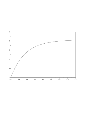
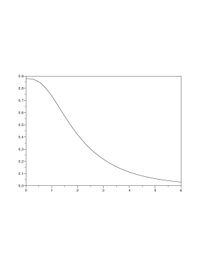
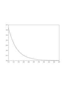
In the Fig. 1, it is shown an example of the shape of $E[\tau(x)],$ given by (3.11), as a function of $x>0$ for $r=x_{R}=1.$

Figure 1: Graph of $E[\tau(x)]$ given by (3.11), as a function of $x>0$ for $r=x_{R}=1$ (on the horizontal axes $x).$

As regards the second order moment of $\tau(x),$ by taking $n=2$ and $U(x)=1$ in (2.11), we get that $T_{2}(x)=E[\tau^{2}(x)]$ is the solution of the problem:

$$\begin{cases}\frac{1}{2}T_{2}^{\prime\prime}(x)-rT_{2}(x)=-\frac{2}{r}e^{x_{R}\sqrt{2r}}(1-e^{-x\sqrt{2r}})-rT_{2}(x_{R})\\ T_{2}(0)=0,\ T_{2}(+\infty)<+\infty.\end{cases}$$ (3.12)

As easily seen, the ODE has general solution

$$T_{2}(x)=c_{1}e^{-x\sqrt{2r}}+c_{2}e^{x\sqrt{2r}}-\frac{2x}{r\sqrt{2r}}e^{-(x-x_{R})\sqrt{2r}}+\frac{2}{r^{2}}e^{x_{R}\sqrt{2r}}+T_{2}(x_{R}),$$ (3.13)

where $c_{1}$ and $c_{2}$ are constants with respect to $x$ to be determined (they depend only on $r$ and $x_{R}).$ From the first boundary condition $T_{2}(0)=0,$ we get

$$c_{1}+c_{2}+\frac{2}{r^{2}}e^{x_{R}\sqrt{2r}}+T_{2}(x_{R})=0;$$ (3.14)

moreover, from $T_{2}(+\infty)<+\infty$ we get $c_{2}=0,$ and so $c_{1}=-\frac{2}{r^{2}}e^{x_{R}\sqrt{2r}}-T_{2}(x_{R}).$

By taking $x=x_{R}$ in (3.13) with $c_{1}=-\frac{2}{r^{2}}e^{x_{R}\sqrt{2r}}-T_{2}(x_{R}),$ we obtain

$$E[\tau^{2}(x_{R})]=e^{x_{R}\sqrt{2r}}\left(\frac{2}{r^{2}}e^{x_{R}\sqrt{2r}}-\frac{2}{r^{2}}-\frac{2x_{R}}{r\sqrt{2r}}\right).$$ (3.15)

Finally, from (3.13):

$$T_{2}(x)=E[\tau^{2}(x)]=e^{x_{R}\sqrt{2r}}\left(\frac{2}{r^{2}}e^{x_{R}\sqrt{2r}}-\frac{2}{r^{2}}-\frac{2x_{R}}{r\sqrt{2r}}\right)\left(1-e^{-x\sqrt{2r}}\right)$$

$$-\frac{2}{r}e^{(x_{R}-x)\sqrt{2r}}\left(\frac{1}{r}+\frac{x}{\sqrt{2r}}\right)+\frac{2}{r^{2}}e^{x_{R}\sqrt{2r}}.$$ (3.16)

This formula can be also found by calculating from (3.5) $\frac{\partial^{2}}{\partial\lambda^{2}}M_{\lambda}(x),$ at $\lambda=0;$ it confirms that the appropriate additional condition must be $T_{2}(+\infty)<\infty.$

In the Fig. 2, it is shown an example of the shape of $E[\tau^{2}(x)],$ given by (3.16), as a function of $x>0$ for $r=x_{R}=1.$

Figure 2: Graph of $E[\tau^{2}(x)]$ as a function of $x>0$ for $r=x_{R}=1$ (on the horizontal axes $x).$

In the Fig. 3, it is shown the shape of $Var[\tau(x)]=E[\tau^{2}(x)]-E^{2}[\tau(x)],$ as a function of $x>0$ for $r=x_{R}=1.$

Figure 3: Graph of $Var[\tau(x)]$ as a function of $x>0$ for $r=x_{R}=1$ (on the horizontal axes $x).$

As regards the behaviors of the first two moments of the FPT $\tau(x)$ for $x\rightarrow 0^{+}$ and $x\rightarrow+\infty,$ from (3.11) we get

$$E[\tau(x)]=a_{1}x+o(x),\ {\rm as}\ x\rightarrow 0^{+},$$ (3.17)

where the constant $a_{1}=\frac{\sqrt{2r}}{r}e^{x_{R}\sqrt{2r}}$ depends on $r$ and $x_{R},$ and

$$\lim_{x\rightarrow+\infty}E[\tau(x)]=a_{1}/\sqrt{2r}.$$ (3.18)

From (3.16) we get that

$$E[\tau^{2}(x)]=a_{2}x+o(x),\ {\rm as}\ x\rightarrow 0^{+},$$ (3.19)

where $a_{2}=\sqrt{2r}E[\tau^{2}(x_{R})]+\frac{\sqrt{2}}{r\sqrt{r}}e^{x_{R}\sqrt{2r}}$ and $E[\tau^{2}(x_{R})]$ is given by (3.15); moreover,

$$\lim_{x\rightarrow+\infty}E[\tau^{2}(x)]=a_{3}.$$ (3.20)

where $a_{3}=E[\tau^{2}(x_{R})]+\frac{2}{r^{2}}e^{x_{R}\sqrt{2r}},$ Thus, we obtain

$$Var[\tau(x)]=a_{2}x+o(x),\ {\rm as}\ x\rightarrow 0^{+},$$ (3.21)

and

$$\lim_{x\rightarrow+\infty}Var[\tau(x)]=a_{4},$$ (3.22)

where $a_{4}=E[\tau^{2}(x_{R})]+\frac{2}{r^{2}}e^{x_{R}\sqrt{2r}}-\frac{1}{r^{2}}e^{2x_{R}\sqrt{2r}}.$

3.2 Moments of the FPA

As shown in [12], [19], [23], [26], the FPA density of Brownian motion with resetting (i.e. for $r>0)$ decays exponentially fast at large values, so the moments of the FPA are finite. The Laplace transform of the FPA, $E[\exp(-\lambda A(x)],$ was obtained in [26] for $x=x_{R}$ in terms of special functions, and the first two moments of the FPA at $x=x_{R}$ were there obtained, by calculating the first and second derivative of $E[\exp(-\lambda A(x_{R})]$ with respect to $\lambda$ at $\lambda=0$ (see Eq. (58) and (59) therein); precisely, it results:

$$E[A(x_{R})]=\frac{x_{R}}{r}e^{x_{R}\sqrt{2r}}:=\alpha_{1}.$$ (3.23)

$$E[A^{2}(x_{R})]=\frac{2e^{x_{R}\sqrt{2r}}}{r}\left[\frac{x_{R}^{2}}{r}\left(\frac{3}{4}+e^{x_{R}\sqrt{2r}}\right)+\frac{1}{r^{2}}-\frac{x_{R}^{3}}{2\sqrt{2r}}\right]-\frac{2}{r^{3}}:=\alpha_{2}.$$ (3.24)

Now, we go to calculate the first two moments of the FPA $A(x)$ for every $x>0,$ by solving the ODE (2.11) with $U(x)=x,$ and $T_{n}(x)=E[A^{n}(x)],n=1,2.$

As regards the mean of $A(x),$ taking $n=1,$ we have that $T_{1}(x)=E[A(x)]$ is the solution of the problem:

$$\begin{cases}\frac{1}{2}T_{1}^{\prime\prime}(x)-rT_{1}(x)=-x-rT_{1}(x_{R})\\ T_{1}(0)=0,\ T_{1}(x_{R})=\alpha_{1},\end{cases}$$ (3.25)

where $\alpha_{1}$ is given by (3.23); note that $A(+\infty)=+\infty,$ so in contrast with the case of the mean FTP the appropriate additional condition is $T_{1}(x_{R})=\alpha_{1}.$ The general solution of the ODE in (3.25) is:

$$T_{1}(x)=c_{1}e^{-x\sqrt{2r}}+c_{2}e^{x\sqrt{2r}}+\frac{x}{r}+\alpha_{1},$$ (3.26)

where $\alpha_{1}$ is given by (3.23), and $c_{1}$ and $c_{2}$ are constants with respect to $x$ to be determined (they depend only on $r$ and $x_{R}).$

From $T_{1}(0)=0,$ we get $c_{1}+c_{2}+\alpha_{1}=0;$ the second condition $T_{1}(x_{R})=\alpha_{1}$ implies $c_{1}e^{-x_{R}\sqrt{2r}}+c_{2}e^{x_{R}\sqrt{2r}}+\frac{x_{R}}{r}=0.$ By solving the system so obtained for $c_{1}$ and $c_{2}$ we obtain $c_{1}=-\frac{1}{r}(e^{x_{R}\sqrt{2r}}x_{R})$ and $c_{2}=0$. Therefore, finally we get:

$$T_{1}(x)=E[A(x)]=\frac{x_{R}}{r}e^{x_{R}\sqrt{2r}}\left(1-e^{-x\sqrt{2r}}\right)+\frac{x}{r}.$$ (3.27)

Remark 3.3

Formula (3.27) extends to all $x>0$ Eq. (58) of [26] which provides $E[A(x_{R})]$ (see (3.23)). Note that, for $r=0$ from Eq. (3.27) it follows $E[A(x)]=+\infty,$ which matches the well-known result for BM (see e.g. [3]).

For $x\rightarrow 0^{+},$ one has $E[A(x)]=\left(\frac{x_{R}\sqrt{2r}}{r}e^{x_{R}\sqrt{2r}}+\frac{1}{r}\right)x+o(x),$ while for large positive $x$ it holds $E[A(x)]\sim\frac{x}{r}.$

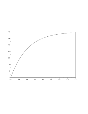
In the Fig. 4, it is shown an example of the shape of $E[A(x)],$ given by (3.27), as a function of $x>0,$ for $r=x_{R}=1.$

Figure 4: Graph of $E[A(x)]$ as a function of $x>0$ for $r=x_{R}=1$ (on the horizontal axes $x).$

As regards the second order moment of $A(x),$ by taking $n=2$ in (2.11) with $U(x)=x,$ we get that $T_{2}(x)=E[A^{2}(x)]$ is the solution of the problem:

$$\begin{cases}\frac{1}{2}T_{2}^{\prime\prime}(x)-rT_{2}(x)=-2xE[A(x)]-rT_{2}(x_{R})\\ T_{2}(0)=0,\ T_{2}(x_{R})=\alpha_{2},\end{cases}$$ (3.28)

where $\alpha_{2}$ is given by (3.24) and $E[A(x)]$ is given by (3.27) (note we have taken the additional condition (3.24)).

Two independent solutions of the homogeneous equation associated to (3.28) are $u_{1}(x)=e^{-x\sqrt{2r}}$ and $u_{2}(x)=e^{x\sqrt{2r}},$ so its general solution is $T_{2}(x)=c_{1}u_{1}(x)+c_{2}u_{2}(x),$ where $c_{1}$ and $c_{2}$ are constants with respect to $x$ to be determined (they depend only on $r$ and $x_{R}).$ By standard methods, we find that a particular solution of (3.28) is

$$\bar{T}_{2}(x)=\frac{2x^{2}}{r^{2}}+\frac{2xx_{R}}{r^{2}}e^{x_{R}\sqrt{2r}}+\frac{2}{r^{3}}+\alpha_{2}-\frac{x_{R}x}{r}e^{-(x-x_{R})\sqrt{2r}}\left(\frac{x}{\sqrt{2r}}+\frac{1}{2r}\right).$$

Thus, the general solution of (3.28) is:

$$T_{2}(x)=c_{1}e^{-x\sqrt{2r}}+c_{2}e^{x\sqrt{2r}}+\bar{T}_{2}(x)=c_{1}e^{-x\sqrt{2r}}+c_{2}e^{x\sqrt{2r}}$$

$$+\frac{2x^{2}}{r^{2}}+\frac{2xx_{R}}{r^{2}}e^{x_{R}\sqrt{2r}}+\frac{2}{r^{3}}+\alpha_{2}-e^{-x\sqrt{2r}}\left(\frac{x_{R}x^{2}}{r\sqrt{2r}}e^{x_{R}\sqrt{2r}}+\frac{x_{R}x}{2r^{2}}e^{x_{R}\sqrt{2r}}\right).$$ (3.29)

By using the boundary condition $T_{2}(0)=0$ and the additional condition $T_{2}(x_{R})=\alpha_{2},$ one gets a system in the unknown $c_{1}$ and $c_{2},$ whose solution is $c_{1}=-\frac{2}{r^{3}}-\alpha_{2},$ and $c_{2}=0.$ Then, inserting into (3.29), one finally obtains:

$$T_{2}(x)=E[A^{2}(x)]=\left(1-e^{-x\sqrt{2r}}\right)\left(\alpha_{2}+\frac{2}{r^{3}}\right)$$

$$+\frac{2x}{r^{2}}\left(x+x_{R}e^{x_{R}\sqrt{2r}}\right)-\frac{x_{R}x}{r}\left(\frac{x}{\sqrt{2r}}+\frac{1}{2r}\right)e^{-(x-x_{R})\sqrt{2r}}.$$ (3.30)

Eq. (3.30) with $\alpha_{2}$ given by (3.24) extends to all value of $x>0$ the formula found in [26] for the expectation of $A^{2}(x_{R})$ (see Eq. (59) therein).

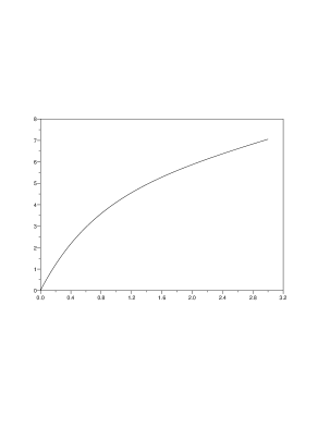
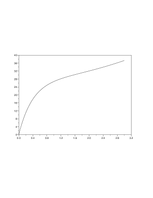
In the Fig. 5, it is shown the shape of $E[A^{2}(x)],$ given by (3.30) as a function of $x>0,$ for $r=x_{R}=1.$ Note that the graph of $E[A^{2}(x)]$ is not globally concave or convex, but it presents an inflection point. In the Fig. 6, it is shown the shape of $Var[A(x)],$ as a function of $x>0,$ for $r=x_{R}=1.$

From (3.30) it follows that, for $x\rightarrow 0^{+},\ E[A^{2}(x)]=\left[\sqrt{2r}\left(\alpha_{2}+\frac{2}{r^{3}}\right)+\frac{3x_{R}}{2r^{2}}e^{x_{R}\sqrt{2r}}\right]x+o(x),$ and $Var[A(x)]$ has the same behavior, at the first order in $x;$ moreover, for large $x>0,$ $E[A^{2}(x)]\sim\frac{2}{r^{2}}x^{2},$ and $Var[A(x)]\sim\frac{x^{2}}{r^{2}}.$

Figure 5: Graph of $E[A^{2}(x)]$ as a function of $x>0$ for $r=x_{R}=1$ (on the horizontal axes $x).$

Figure 6: Graph of $Var[A(x)],$ as a function of $x>0$ for $r=x_{R}=1$ (on the horizontal axes $x).$

Remark 3.4

From the previous calculations, we conclude that the following growth conditions (upper bounds) hold:

$$E[A(x)]\leq const\cdot x,\ {\rm for\ large}\ x>0,$$ (3.31)

and

$$E[A^{2}(x)]\leq const^{\prime}\cdot x^{2},\ {\rm for\ large}\ x>0.$$ (3.32)

Note that similar bounds holds for Brownian motion with negative drift $\mu$ (without resetting, i.e. $r=0),$ because in that case the moments of $A(x)$ grow at most polynomially in $x$ (see [3]).

3.3 Joint moment of $A(x)$ and $\tau(x)$

In this subsection we find an explicit expression for $E[A(x)\tau(x)],$ i.e. the joint moment of $A(x)$ and $\tau(x).$ The joint LT of $\tau(x),A(x)$ is

$$M_{\lambda_{1},\lambda_{2}}(x)=E\left[e^{-\lambda_{1}\tau(x)}e^{-\lambda_{2}A(x)}\right],\lambda_{1},\lambda_{2}>0.$$

By reasoning as before (see Proposition 2.1), we find that it satisfies the differential equation:

$$(L-r)M_{\lambda_{1},\lambda_{2}}(x)=(\lambda_{1}+\lambda_{2}x)M_{\lambda_{1},\lambda_{2}}(x)-rM_{\lambda_{1},\lambda_{2}}(x_{R}).$$ (3.33)

Then, by taking $\frac{\partial^{2}}{\partial\lambda_{1}\partial\lambda_{2}}$ in both members of Eq. (3.33) and calculating it at $\lambda_{1}=\lambda_{2}=0,$ we obtain that $V(x):=E[\tau(x)A(x)]$ satisfies the differential problem:

$$(L-r)V(x)=-xE[\tau(x)]-E[A(x)]-rV(x_{R}),\ V(0)=0,$$ (3.34)

with a suitable additional condition. Actually, since $E[A(x)\tau(x)]\leq\sqrt{E[A^{2}(x)]}\sqrt{E[\tau^{2}(x)]},$ by using (3.20) and (3.32), one obtains that the additional condition for the ODE (3.34) must be:

$$V(x)=E[\tau(x)A(x)]\leq const\cdot x,\ {\rm for\ large}\ x>0.$$ (3.35)

By standard methods, we find that the general solution of (3.34) is:

$$V(x)=c_{1}e^{-x\sqrt{2r}}+c_{2}e^{x\sqrt{2r}}+\bar{V}(x),$$

where $c_{1}$ and $c_{2}$ are constants with respect to $x$ to be determined (they depend only on $x_{R}$ and $r),$ and

$$\bar{V}(x)=\frac{(e^{x_{R}\sqrt{2r}}+1)x}{r^{2}}+\frac{x_{R}e^{x_{R}\sqrt{2r}}}{r^{2}}-e^{-(x-x_{R})\sqrt{2r}}\left(\frac{x^{2}}{2r\sqrt{2r}}+\frac{(1+2x_{R}\sqrt{2r})x}{4r^{2}}\right)+V(x_{R})$$ (3.36)

is a particular solution of (3.34). By imposing the condition $V(0)=0,$ one gets

$$0=c_{1}+c_{2}+\bar{V}(0)$$ (3.37)

By using (3.35), we find that $c_{2}$ must be zero, so $c_{1}=-\frac{x_{R}e^{x_{R}\sqrt{2r}}}{r^{2}}-V(x_{R}),$ and we obtain:

$$V(x)=-\left[\frac{x_{R}e^{x_{R}\sqrt{2r}}}{r^{2}}+V(x_{R})\right]e^{-x\sqrt{2r}}+\bar{V}(x).$$ (3.38)

By taking $x=x_{R}$ in (3.38), one obtains an equation in the unknown $V(x_{R})$ whose solution provides:

$$V(x_{R})=e^{x_{R}\sqrt{2r}}\left[\left(8e^{x_{R}\sqrt{2r}}-1\right)\frac{x_{R}}{4r^{2}}-\frac{3x_{R}^{2}}{2r\sqrt{2r}}\right].$$ (3.39)

Finally, the expression for $V(x)=E[\tau(x)A(x)]$ follows from (3.38), (3.36) and (3.39).

By using (3.11), (3.27) and (3.39), the expressions of $Cov[A(x),\tau(x)]:=V(x)-E[\tau(x)]E[A(x)]$ and of the correlation coefficient

$$\rho_{\tau(x),A(x)}:=\frac{Cov[\tau(x),A(x)]}{\sqrt{Var[\tau(x)]Var[A(x)]}},$$ (3.40)

soon follow.

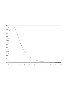
As easily seen by examination of the various quantities involved, $\rho_{\tau(x),A(x)}$ turns out to be positive for every $x>0,$ that is, $\tau(x)$ and $A(x)$ are positively correlated; moreover, $\lim_{x\rightarrow 0^{+}}\rho_{\tau(x),A(x)}=\rho_{0}>0,$ and $\lim_{x\rightarrow+\infty}\rho_{\tau(x),A(x)}=\rho_{\infty}<\rho_{0}.$ The graph of $\rho_{\tau(x),A(x)}$ increases from $\rho_{0}$ to a maximum value, after that it decreases to $\rho_{\infty}<\rho_{0},$ as $x\rightarrow+\infty.$ This kind of behavior for $\rho_{\tau(x),A(x)}$ was also observed for drifted BM without reset (see [3]) and Onrstein-Uhlenbeck process without reset (see [5]).

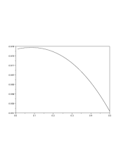
In the Fig. 7, first panel, we show the graph of $\rho_{\tau(x),A(x)},$ as a function of $x>0$ for $r=x_{R}=1$ (on the horizontal axes $x);$ the existence of the maximum is revealed by an enlargement around $x=0.1\$ (second panel). Fig. 8 shows another example of the graph of $\rho_{\tau(x),A(x)},$ obtained for $r=1$ and $x_{R}=2.$

Figure 7: Graph of $\rho_{\tau(x),A(x)}$ as a function of $x>0$ for $r=x_{R}=1$ (on the horizontal axes $x);$ in the second panel it is shown an enlargement around $x=0.1\ .$

Figure 8: Graph of $\rho_{\tau(x),A(x)}$ as a function of $x>0$ for $r=1$ and $x_{R}=2.$ (on the horizontal axes $x).$

3.4 Maximum displacement

We define the maximum displacement of BM with resetting ${\cal X}(t),$ starting from $x>0,$ as the r.v. ${\cal M}_{x}=\max_{t\in[0,\tau(x)]}{\cal X}(t)$ (obviously we have ${\cal M}_{x}\geq x).$ Note that the event $\{{\cal M}_{x}\leq z\}$ occurs if and only if ${\cal X}(t)$ first exits the interval $(0,z)$ through the left end $0.$ Therefore, for $z\geq x$ one gets that the distribution function $F_{{\cal M}_{x}}(z)=P({\cal M}_{x}\leq z)$ is the solution of the differential equation (see e.g. [2], [5]):

$$\begin{cases}{\cal L}w(x)=\frac{1}{2}w^{\prime\prime}(x)+rw(x_{R})-rw(x)=0,\ x\in(0,z)\\ w(0)=1,\ w(z)=0,\end{cases}$$ (3.41)

where ${\cal L}$ is the infinitesimal generator of ${\cal X}(t)$ (see (1.2)). The general solution of the associated homogeneous equation is $w_{0}(x)=c_{1}e^{-x\sqrt{2r}}+c_{2}e^{x\sqrt{2r}},$ where for fixed $x$ and $x_{R},$ $c_{i}=c_{i}(z)$ are indeed functions of $z,$ while a particular solution is $\bar{w}(x)=a=w(x_{R}),$ where $a=a(z)$ is a function of $z;$ therefore, the general solution of (3.41) is

$$w(x)=c_{1}e^{-x\sqrt{2r}}+c_{2}e^{x\sqrt{2r}}+a,$$ (3.42)

where the functions $c_{1},\ c_{2}$ and $a$ are to be found. By imposing the boundary conditions, and taking $x=x_{R}$ in (3.42), we obtain that $c_{1}(z),\ c_{2}(z)$ and $a(z)$ must satisfy the system:

$$\begin{cases}c_{1}+c_{2}+a=1\\ c_{1}e^{-z\sqrt{2r}}+c_{2}e^{z\sqrt{2r}}+a=0\\ c_{1}e^{-x_{R}\sqrt{2r}}+c_{2}e^{x_{R}\sqrt{2r}}=0.\end{cases}$$ (3.43)

By solving the above system, one finds:

$$\begin{cases}c_{1}=c_{1}(z)=(e^{z\sqrt{2r}}-1)^{-1}(e^{-z\sqrt{2r}}+e^{-2x_{R}\sqrt{2r}})^{-1}\\ c_{2}=c_{2}(z)=-e^{-2x_{R}\sqrt{2r}}c_{1}\\ a=a(z)=1-c_{1}(z)-c_{2}(z).\end{cases}$$ (3.44)

Finally, we get

$$F_{{\cal M}_{x}}(z)=P({\cal M}_{x}\leq z)=\begin{cases}0,\ \ \ \ \ \ \ \ \ \ \ \ \ \ \ \ \ \ \ \ \ \ \ \ \ \ \ \ \ \ \ \ \ \ \ z<x\\ c_{1}(z)e^{-x\sqrt{2r}}+c_{2}(z)e^{x\sqrt{2r}}+a(z),\ z\geq x.\end{cases}$$ (3.45)

where $c_{i}(z)$ and $a(z)=w(x_{R})$ are given by (3.44). As we see, the distribution function of ${\cal M}_{x}-x$ appears to have a tail that decays exponentially fast, and so the expectation $E[{\cal M}_{x}]$ results to be finite. By calculating the solution of (3.41) for $r=0,$ we obtain that, for BM without resetting the distribution of the maximum displacement is (see also [7]):

$$F_{{\cal M}_{x}}(z)=\begin{cases}0,\ \ \ \ \ \ \ z<x\\ 1-\frac{x}{z},\ z\geq x,\end{cases}$$ (3.46)

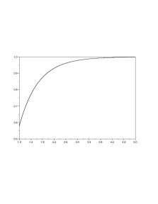
which implies that the expectation of the maximum displacement of BM without resetting is infinite. In the Fig 9 it is shown an example of the distribution function of the maximum displacement ${\cal M}_{x}$ of BM with resetting, and the corresponding probability density, obtained by taking the derivative in (3.45), for $x=1,x_{R}=0.5$ and $r=1.$

Figure 9: Left panel: distribution function of the maximum displacement ${\cal M}_{x}$ of BM with resetting, for $x=1,x_{R}=0.5$ and $r=1;$ right panel: the corresponding density (on the horizontal axes $z\geq x=1).$

4 Drifted Brownian motion with resetting

In this section, we consider drifted Brownian motion with resetting ${\cal X}(t),$ precisely we suppose that the underlying diffusion process is Brownian motion with drift $\mu,$ that is $X(t)=x+B_{t}+\mu t,$ and we find explicit expressions of the LT, the moments of FPT and FPA, and the maximum displacement of ${\cal X}(t),$ as solutions of differential problems. Since many calculations are analogous to those of the undrifted case, we omit the details, reporting only the results.

Note that the FPT trough zero of Brownian motion with non-zero drift $\mu$ (without resetting) starting from $x>0$ is finite with probability one, only if the drift is negative; instead, the FPT trough zero of drifted Brownian motion with resetting ${\cal X}(t)$ is finite, irrespective of the sign of the drift $\mu$ and the moments of FPT are also finite, for any $0<r<+\infty$ (see e.g. [23]).

The infinitesimal generator of $X(t)$ is now given by $Lf(x)=\frac{1}{2}\frac{df^{2}}{dx^{2}}+\mu\frac{df}{dx};$ by proceeding as in the case of undrifted Brownian motion with resetting, the solutions of the various equations cam be obtained by taking $\mu+\sqrt{\mu^{2}+2(\lambda+r)}$ in place of $\sqrt{2(\lambda+r)}$ in the corresponding formulae.

4.1 The Laplace transform of $\tau(x)$

The Laplace transform of $\tau(x)$ turns out to be:

$$M_{\lambda}(x)=E\left[e^{-\lambda\tau(x)}\right]=e^{-x\left(\mu+\sqrt{\mu^{2}+2(\lambda+r)}\ \right)}+M_{\lambda}(x_{R})\frac{r}{\lambda+r}\left(1-e^{-x\left(\mu+\sqrt{\mu^{2}+2(\lambda+r)}\ \right)}\right),$$ (4.1)

where

$$M_{\lambda}(x_{R})=\frac{(\lambda+r)e^{-x_{R}\left(\mu+\sqrt{\mu^{2}+2(\lambda+r)}\ \right)}}{\lambda+re^{-x_{R}\left(\mu+\sqrt{\mu^{2}+2(\lambda+r)}\ \right)}}$$ (4.2)

Remark 4.1

Formula (4.1) appears to be new, because in [26] it was studied only undrifted Brownian motion with resetting. For $\mu=0$ (4.1) and (4.2) provide again (3.5) and (3.4).

4.2 The Laplace transform of $A(x)$

Unfortunately, the corresponding ODE cannot be solved in terms of elementary functions, having non costant coefficients.

4.3 Moments of the FPT

The mean of the FPT is:

$$E[\tau(x)]=\frac{1}{r}e^{x_{R}(\mu+\sqrt{\mu^{2}+2r})}\left(1-e^{-x(\mu+\sqrt{\mu^{2}+2r})}\right).$$ (4.3)

For $\mu=0,$ we obtain again (3.11).

As for the second order moment of $\tau(x),$ one has:

$$E[\tau^{2}(x)]$$

$$=e^{x_{R}(\mu+\sqrt{\mu^{2}+2r})}\left(\frac{2}{r^{2}}e^{x_{R}(\mu+\sqrt{\mu^{2}+2r})}-\frac{2}{r^{2}}-\frac{2x_{R}}{r\sqrt{\mu^{2}+2r}}\right)\left(1-e^{-x(\mu+\sqrt{\mu^{2}+2r})}\right)$$

$$-\frac{2}{r}e^{(x_{R}-x)(\mu+\sqrt{\mu^{2}+2r})}\left(\frac{1}{r}+\frac{x}{\sqrt{\mu^{2}+2r}}\right)+\frac{2}{r^{2}}e^{x_{R}(\mu+\sqrt{\mu^{2}+2r})}.$$ (4.4)

For $\mu=0,$ we obtain again (3.16).

4.4 Moments of the FPA

The mean of the FPA turns out to be:

$$E[A(x)]=E[A(x_{R})]\left(1-e^{-x\left(\mu+\sqrt{\mu^{2}+2r}\ \right)}\right)+\frac{x}{r}+\frac{\mu}{r^{2}}\left(1-e^{-x\left(\mu+\sqrt{\mu^{2}+2r}\ \right)}\right),$$ (4.5)

where

$$E[A(x_{R})]=e^{x_{R}\left(\mu+\sqrt{\mu^{2}+2r}\ \right)}\left[\frac{x_{R}}{r}+\frac{\mu}{r^{2}}\left(1-e^{-x_{R}\left(\mu+\sqrt{\mu^{2}+2r}\ \right)}\right)\right].$$ (4.6)

For $\mu=0,$ we obtain again $E[A(x_{R})]=\frac{x_{R}}{r}e^{\sqrt{2r}x_{R}}$ and $T_{1}(x)=\frac{x_{R}}{r}e^{\sqrt{2r}x_{R}}(1-e^{-x\sqrt{2r}})+\frac{x}{r}$ (see (3.23) and (3.27).

As for the second order moment of $A(x),$ in principle, it is possible to find the explicit solution of the corresponding ODE, by proceeding as in the case of undrifted BM with resetting; however the calculations are far heavier and the form of the explicit solution is cumbersome to be written here. Its qualitative behavior can be studied by making use of a software for numerical solutions of linear ODEs of the second order.

4.5 Maximum displacement

The distribution function of the maximum displacement ${\cal M}_{x}$ turns out to be:

$$F_{{\cal M}_{x}}(z)=P({\cal M}_{x}\leq z)=\begin{cases}0,\ \ \ \ \ \ \ \ \ \ \ \ \ \ \ \ \ \ \ \ \ \ \ \ \ \ \ \ \ \ \ \ \ \ \ z<x\\ c_{1}(z)e^{d_{1}x}+c_{2}(z)e^{d_{2}x}+a(z),\ z\geq x.\end{cases}$$ (4.7)

where $d_{1}=-\mu-\sqrt{\mu^{2}+2r}<0,\ d_{2}=-\mu+\sqrt{\mu^{2}+2r}>0,$ and the functions $c_{i}(z)$ and $a(z)$ are given by:

$$\begin{cases}c_{1}(z)=-\left[e^{-\left(\mu+\sqrt{\mu^{2}+2r}\ \right)z}-1+e^{-2x_{R}\sqrt{\mu^{2}+2r}}\left(1-e^{-\left(\mu-\sqrt{\mu^{2}+2r}\ \right)z}\right)\right]^{-1}\\ c_{2}(z)=-c_{1}e^{-2x_{R}\sqrt{\mu^{2}+2r}}\\ a(z)=1-c_{1}(z)-c_{2}(z).\end{cases}$$ (4.8)

For $\mu=0$ (4.7) becomes (3.45). Once again, the distribution function of ${\cal M}_{x}-x$ has a tail that decays exponentially fast, and so the expectation $E[{\cal M}_{x}]$ results to be finite. Note that for Brownian motion with drift $\mu<0$ (without resetting) the distribution of the maximum displacement is (see also [7]):

$$F_{{\cal M}_{x}}(z)=\begin{cases}0,\ \ \ \ \ \ \ \ \ \ z<x\\ \frac{e^{-2\mu x}-e^{-2\mu z}}{1-e^{-2\mu z}},\ z\geq x,\end{cases}$$ (4.9)

and its density is

$$f_{{\cal M}_{x}}(z)=\begin{cases}0,\ \ \ \ \ \ \ \ \ \ z<x\\ \frac{\mu e^{-\mu x}\sinh(\mu x)}{\sinh^{2}(\mu z)},\ z\geq x,\end{cases}$$ (4.10)

from which it follows that, unlike the case $\mu=0,$ the expectation of the maximum displacement of BM with drift $\mu<0$ is $E[{\cal M}_{x}]=x-\frac{1-e^{-2\mu x}}{2\mu}\ln\left(1-e^{2\mu x}\right)<+\infty$.

Note that, for $\mu\rightarrow 0^{-}$ the last expression tends to $+\infty$ (see the comment after (3.46)).

5 Conclusions and final remarks

We have studied a one-dimensional Wiener process with stochastic resetting ${\cal X}(t)$, obtained from an underlying drifted Brownian motion $X(t)=x+\mu t+B_{t},$ starting from $x>0,$ where $B_{t}$ is standard Brownian motion, and the drift $\mu$ is non positive. We have supposed that resetting events occur according to a homogeneous Poisson process with rate $r>0;$ until the first resetting event the process ${\cal X}(t)=X(t)$ evolves as a Brownian motion with drift with ${\cal X}(0)=X(0)=x>0;$ when the reset occurs, ${\cal X}(t)$ is set instantly to a position $x_{R}>0.$ After that, ${\cal X}(t)$ evolves again as Brownian motion with drift, starting afresh (independently of the past history) from $x_{R},$ until the next resetting event occurs, and so on. The inter-resetting times turn out to be independent and exponentially distributed random variables with parameter $r.$ We have studied the statistical properties of the first-passage time (FPT) of ${\cal X}(t)$ through zero, when starting from $x>0,$ and its first-passage area (FPA) (i.e. the random area enclosed between the time axis and the path of the process ${\cal X}(t)$ up to the FPT through zero). By solving certain associated ODEs, we have obtained explicitly the Laplace transform of the FPT and the FPA of ${\cal X}(t),$ and their single and joint moments; moreover, we have provided the distribution of the maximum displacement of ${\cal X}(t).$ The calculations have been shown in some detail only in the case $\mu=0;$ for $\mu\neq 0$ we have only reported the corresponding formulae.

Notice that some results, regarding undrifted Brownian motion with stochastic resetting, were already obtained in [26], by using special functions.

We emphasize that, as regards the FPT of drifted Brownian motion with resetting ${\cal X}(t)$, the main qualitative difference with the case of the drifted Brownian motion $X(t)$ (without resetting) is that the FPT of ${\cal X}(t)$ through zero is finite and it has finite expectation for every $x>0,$ whilst the mean of the FPT of $X(t)$ is finite only for $\mu<0,$ being infinite for $\mu=0,$ though the hitting time to zero of Brownian motion starting from $x>0$ is finite with probability one. Actually, the FPT density of Brownian motion decays as $t^{-3/2}$ at large time $t.$ In contrast, both the FPT density and the FPA density of Brownian motion with resetting decay exponentially fast at large values (see e.g. [12], [23], [26]), and so the moments of FPT and FPA result to be finite.

In principle, the arguments of this paper can be used to obtain differential equations for the Laplace transforms, the moments of FPT and FPA and the distribution of the maximum displacement also for other diffusion processes with stochastic resetting, such as the Ornstein-Uhlenbeck process with stochastic resetting (see e.g. [11]), namely when the underling process is the diffusion $X(t)=X_{OU}(t)$ which is driven by the SDE $dX(t)=-\nu X(t)+\sigma dB_{t},$ for positive constants $\nu$ and $\sigma.$ For instance, if $\tau$ denotes again the FPT of $X_{OU}(t)$ through zero, when starting from $x>0,$ then $T(x)=E[\tau(x)]$ turns out to be solution to:

$$\begin{cases}\frac{1}{2}T^{\prime\prime}(x)-\nu xT^{\prime}(x)-rT(x)=-1-rT(x_{R})\\ T(0)=0,\ T_{1}(+\infty)<\infty.\end{cases}$$ (5.1)

The additional condition $T_{1}(+\infty)<\infty$ can be replaced by $\lim_{\nu\rightarrow+\infty}T(x)=0.$

The differential equation above is complicated enough, but it can be solved in principle in the following way. Let $\psi(x)=E[e^{-r\tau_{OU}(x)}]$ be the Laplace transform of $\tau_{OU}(x),$ which is explicitly given by Eq. (3.49) of [5] in terms of a cylinder parabolic function. Then, we search for a solution to (5.1) of the form $T(x)=\psi(x)v(x),$ where $v(x)$ is a function to be determined. By calculating first and second derivatives and inserting into (5.1) one obtains the ODE:

$$\frac{1}{2}\psi(x)v^{\prime\prime}(x)+v^{\prime}(x)(\psi^{\prime}(x)-\nu x\psi(x))=c,$$

with $c=-1-rT(x_{R}),$ that can be solved by quadratures, in the unknown function $v(x),$ and so $E[\tau(x)]=T(x)=\psi(x)v(x)$ can be obtained. Analogous way can be followed in principle to solve the differential equations for the LT of $\tau(x)$ and the mean of $A(x).$

Note that in [11] the explicit expressions of the LT of the FPT $\tau(x)$ of Ornstein-Uhlenbeck process with stochastic resetting and its mean $E[\tau(x)]$ were explicitly obtained in terms of special functions.