Benchmark data to study the influence of pre-training
on explanation performance in MR image classification
Abstract
Convolutional Neural Networks (CNNs) are frequently and successfully used in medical prediction tasks. They are often used in combination with transfer learning, leading to improved performance when training data for the task are scarce. The resulting models are highly complex and typically do not provide any insight into their predictive mechanisms, motivating the field of ‘explainable’ artificial intelligence (XAI). However, previous studies have rarely quantitatively evaluated the ‘explanation performance’ of XAI methods against ground-truth data, and transfer learning and its influence on objective measures of explanation performance has not been investigated. Here, we propose a benchmark dataset that allows for quantifying explanation performance in a realistic magnetic resonance imaging (MRI) classification task. We employ this benchmark to understand the influence of transfer learning on the quality of explanations. Experimental results show that popular XAI methods applied to the same underlying model differ vastly in performance, even when considering only correctly classified examples. We further observe that explanation performance strongly depends on the task used for pre-training and the number of CNN layers pre-trained. These results hold after correcting for a substantial correlation between explanation and classification performance.
1 Introduction
Following AlexNet’s [23] victory in the ImageNet competition, CNNs developed to become the deep neural network (DNN) architecture of choice for any image-based prediction tasks. Apart from their ingenious design, the success of CNNs was made possible by ever-growing supplies of data and computational resources.
However, sufficient labelled data to train complex CNNs are not widely available for every prediction task. This is especially true for medical imaging data, which is cumbersome to acquire and underlies strict data protection regulations. To address this bottleneck, Transfer Learning (TL) techniques are frequently employed [2]. In the context of DNNs, TL strategies often consist of two steps. First, a surrogate model is trained on a different prediction tasks, for which ample training data are available. This is called pre-training. And, second, the resulting model is adapted to the prediction task of interest, where only parts of the model’s parameters are updated , while other parameters are kept untouched. [27]. This is called re-training or fine-tuning and requires smaller amounts of labelled data than training a network from scratch, leading to a less computationally expensive process. It is believed that TL techniques improves the generalisation by identifying common features between the two tasks [38]. Also, TL is frequently employed for prediction tasks in medical imaging. Cheng and Malhi [6] use a DNN, trained with the ImageNet dataset [11], to classify ultrasound images into eleven categories, achieving better results than human radiologists. Another example is the reconstruction of Magnetic Resonance Imaging (MRI) data with models trained on an image corpus that was augmented with ImageNet data [8]. The resulting model outperformed conventional reconstruction techniques. However, it also has been argued [30] that the use of pre-trained models may not be adequate for the medical field. The main argument being that structures in medical images are very different from those observed in natural images. Hence, feature representations learned during pre-training may not be useful for solving clinical tasks.
Despite the success of DNN models, their intrinsic structure makes them hard to interpret. This challenges their real-world applicability in high-stake fields such as medicine. Although many practices in medicine are still not purely evidence-based, the risk posed by faulty algorithms is exponentially higher than that of doctor–patient interactions [37]. Thus, it has been recognised that the working principles of complex learning algorithms need to be made transparent if such algorithms are to be used on critical human data. The General Data Protection Regulation of the European Union (GDPR, Article 15), for example, states that patients have the right to receive meaningful information about how decisions are achieved based on their data, including decisions made based on artificial intelligence algorithms, such as DNNs [14].
The field of ‘explainable artificial intelligence’ (XAI) originated to address this need. Several XAI methods seek to deliver ‘post-hoc explanations’, where explanations are obtained after a model has been trained and applied to a test input. The outcome of such methods is often a so-called heat map, which assigns ‘importance’ scores to the input features. However, despite the popularity of various XAI methods – accumulating thousands of citations within a few years – their theoretical underpinnings are far from established. Most importantly, there is no agreed upon definition of what explainability means or what XAI methods are supposed to deliver [44]. Consequently, little quantitative empirical validation of XAI methods [9] exists. The lack of robust quantitative criteria to benchmark XAI methods against ground-truth data is problematic and speaks against their use in critical domains. It also means that, when highly unstable results for identical inputs occur, it is impossible to judge which one is more accurate.
One step towards overcoming this issue is to devise working definitions of what constitutes a ground-truth explanation. Such a definition would allow us to measure the explanation performance of XAI methods using objective metrics. So far, most quantitative studies in the XAI field focus on secondary quality aspects such as robustness or uncertainty but spare out the fundamental issue of correctness, which should be the prime concern before looking into any secondary metrics such as stability. Recently, however, the field has moved towards a more objective validation of XAI approaches using synthetic data [36, 43, 3, 17, 1]. Wilming et al. [41], for example, provide a data-driven definition of explainability as well as quantitative metrics to measure explanation performance. Their empirical evaluation of a large number of XAI approaches is, however, limited to linear toy data. On the other hand, [20] used XAI methods to find structural changes of the ageing brain, which allowed the authors to identify white matter lesions associated to the ageing brain and forms of dementia. The obtained heat maps were compared with the lesion maps. Cherti and Jitsev [7] analysed pre-training as well, while fine-tuning their models to predict the age of a brain. They explained the model using LRP [5] and compared the resulting heat maps with white matter lesion maps created using the lesion segmentation toolbox by Schmidt et al. [29].
In this work, we extend these lines of research in one major aspect. We devise ground-truth data for a realistic clinical use case, the classification of brain MRIs, according to the presence of different lesion types. To this end, we overlay real MR images with artificial lesions, loosely resembling white matter hyperintensities (WMH). WMH are important biomarkers of the aging brain and ageing-related neurodegenerative disorders [40, 12]. We establish a realistic use case for an MRI prediction task, and more importantly, provide a ground-truth benchmark for model explanations in this task, as the positions of the artificial lesions defining solely the class-membership are fully known by construction. In the second part of this work, we show the benchmark’s utility by investigating both classification as well as explanation performance as a function of pre-training. We provide a framework for generating MRI slices with different types of lesions and respective ground-truths. We then use this framework to benchmark common XAI methods against each other and to compare the explanation performance of models pre-trained using either within-domain data (using different MRI classification tasks) or out-of-domain data (using natural images from the ImageNet classification challenge [10]).
2 Methods
2.1 Data Generation
To generate the data used for this analysis, we use 2-dimensional T1-weighted axial MRI slices from 1007 healthy adults aged between 22 and 37 years, sourced from the Human Connectome Project (HCP) [39] (see also supplemental material section A). The MRI data consists of 3D MRI slices pre-processed with FSL [22] and FreeSurfer [15] tools [18, 21] and defaced through the algorithm reported in Milchenko and Marcus [25]. These slices provide the background on which a random number of artificial ‘lesions’ are overlaid. Regular and irregular lesions are generated and added to the slices. Each slice contains only one type of lesions. This defines a binary classification problem, which we solve using CNNs. The lesions are added so that the dataset created is balanced.
For this study, we keep only slices with less than 55% black pixels. These images are 260311 pixels in size. To obtain square images, they are padded vertically with zeros and cropped horizontally. The final size of the slices result in background images , where we keep the intensity values for .
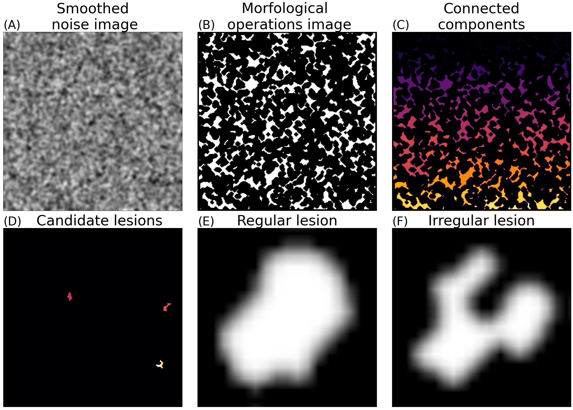
Artificial lesions are created from a 256256 pixel noise image, to which a Gaussian filter with a radius of 2 pixels is applied. The Otsu method [26] is used to binarise the smoothed image. After the application of the morphological operations erosion and opening, a second erosion is applied to create more irregular shapes (see supplemental material section C). Since these shapes occur less frequently than regular shapes, these determine the number of different noise images necessary to create a given number of lesions.
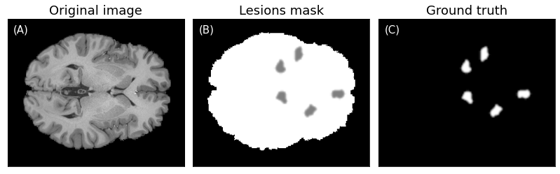
From the images obtained after the application of the morphological operations, the connected components (contiguous groups of non-zero intensity pixels fully surrounded by zero intensity pixels) are identified, which serve as lesion candidates. Further, lesions are selected based on the compactness of their shape. Here, it is sufficient to consider the isoperimetric inequality on a plane , where is the area of a particular lesion shape and its perimeter. The compactness is obtained by comparing the shape of the lesion candidate to a circle with the same perimeter. The larger the compactness, the rounder the shape. Here, regular lesions are required to have a compactness above and irregular lesions have a compactness below . After selecting the lesions, they are padded with a 2-pixel margin, and a Gaussian filter with a radius of pixels is applied to smooth the lesion boundaries. Examples of obtained lesions are displayed in Figure 1.
Three to five lesions of the same type (regular or irregular) are composed in one image in random locations within the brain, without overlapping and pixel-wise multiplied with the background MRI (see Figure 2). For the lesions we consider the intensity values , where correspond to pixels representing lesions. The parameter is a constant that controls the SNR. Higher values lead to whiter lesions and higher SNR, leading to easier classification and explanation tasks. In this study, we set . Note also, that this setup may lead to the emergence of so-called suppressor variables. These would be pixels of the background outside any lesion, which could still provide a model with information on how to remove background content from lesion areas in order to improve the model’s predictions. Suppressor variables have been shown to be often misinterpreted for important class-dependent features by XAI methods [19, 41].
In parallel to the generation of the actual synthetic MR images, the same lesions are added to a black image to create ground-truth masks. Examples of these created images can be seen in Figure 2 (C).
Out of the subjects in the HCP dataset, 60% were used to create the training dataset, 20% to create the validation dataset, and another 20% to create the holdout dataset, corresponding to , , and slices, respectively.
2.2 Pre-training
We apply the XAI methods to the VGG-16 [32] architecture, included in the Torchvision package, version 0.12.0+cu102. Two models are pre-trained using two different corpora, and serve as starting points for our study. The first model is pre-trained using the ImageNet dataset [11] (out-of-domain pre-training). The weights used are included in the same version of Torchvision. The second model is pre-trained using MRI slices extracted from the HCP as described before but without artificial lesions (within-domain pre-training). Here, the task is to classify slices according to whether they were acquired from female or male subjects. To train the latter model, slices are used, 46% of which belong to male subjects and 54% to female subjects. These slices are arranged into batches of 32 data points. The model is trained using stochastic gradient decent (SGD) with a learning rate (LR) of 0.02 and momentum of 0.5. The learning rate is reduced by 10% every 5 epochs. Cross-entropy is used as the loss function.
2.3 Fine-tuning
After pre-training, the models are fine-tuned layer-wise on the lesion-classification problem, with images chosen from the holdout dataset, which we split into train/validation/test again (see supplementary material section D). Each degree of fine-tuning includes the convolutional layers between two consecutive max-pooling layers. Thus, the five degrees of fine-tuning are: 1conv (fine-tuning up to the first max-pooling layer), 2conv (fine-tuning up to the second max-pooling layer), and so on, up to all (fine-tuning of all VGG-16 layers). Weights in layers that are not to be fine-tuned are frozen. SGD and Cross-entropy loss with the same parameters as used for the pre-training are employed in this phase. However, several different LRs are used.
2.4 XAI methods
We apply XAI methods from the Captum library (version 0.5.0). These methods have been proposed to provide ‘explanations’ of the models’ output in the form of a heat map , assigning an ‘importance’ score to each input feature of an example. We use the default settings from Captum for all XAI methods. Wherever a baseline – a reference point to begin the computation of the explanation – is needed, an all-zeros image is used. This is done for Integrated Gradients, DeepLift, and GradientSHAP. The absolute value of the obtained importance score or heat map constitutes the basis for our visualisations and quantitative explanation analyses. For visualisation purposes, we further transformed the intensity of the importance scores by , where is the natural logarithm and . The XAI methods used were Integrated Gradients [35], Gradient SHAP [24], Layer-wise Relevance Propagation (LRP) [4], DeepLIFT [31], Saliency [33], Deconvolution [42] and Guided Backpropagation [34].
2.5 Explanation performance
Our definition of quantitative explanation performance is the precision to which the generated importance or heat maps resemble the ground-truth, i.e. the location of the lesions (cf. Figure 2). It would be expected that the best explanation would only highlight the pixels of the ground-truth, since those are the ones that are relevant to the classification task at hand. We determine the explanation performance by finding the most intense pixels of the heat map , where is equal to the number of pixels in the ground-truth of each image. Then we calculate the number of these pixels that were in the ground-truth (true positives). The precision is obtained by calculating the ratio between the true positives and all positives (the number of pixels in the ground-truth).
2.6 Baselines
The performance of each explanation is then compared to several baseline methods, which act as ‘null models’ for explanation performance. These baselines are models that are initialised randomly and not trained (random model) and two edge detection methods, the Laplace and Sobel filters.
3 Experiments
Showcasing the proposed dataset’s utility, we fine-tune two VGG-16 models that have been previously pre-trained with the two corpora (ImageNet and MRI), to five different degrees. For each degree of fine-tuning, we fine-tuned 15 models with different seeds. Then we select the three best-performing models, where performance is measured on test data in terms of accuracy. We further analyse the model explanation performance of common XAI methods with respect to the ground-truth explanations in the form of lesion maps provided by our dataset. A reference to the Python code to reproduce our experiments is provided in the supplemental material section B.
4 Results
The best-performing models had an accuracy above 90% except the least fine-tuned ones (1conv). All models, except the least fine-tuned ones (1conv), reached accuracies above 90%. The models pre-trained with ImageNet achieved higher accuracy than the ones pre-trained with MR images.
4.1 Qualitative analysis of explanations
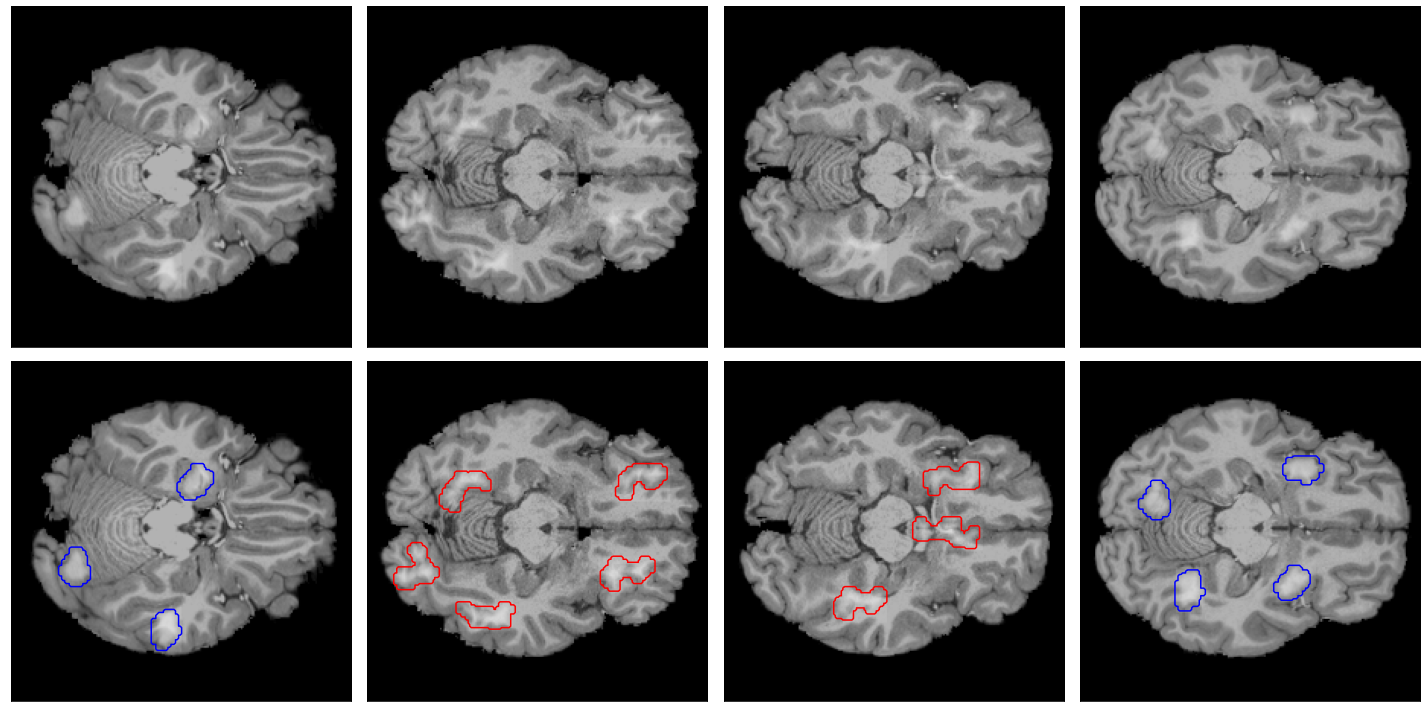
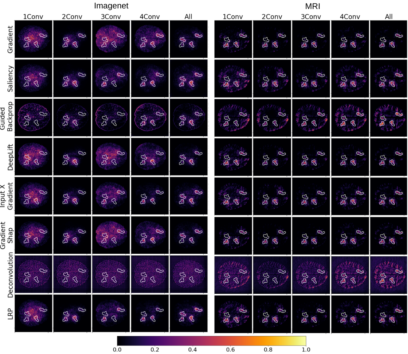
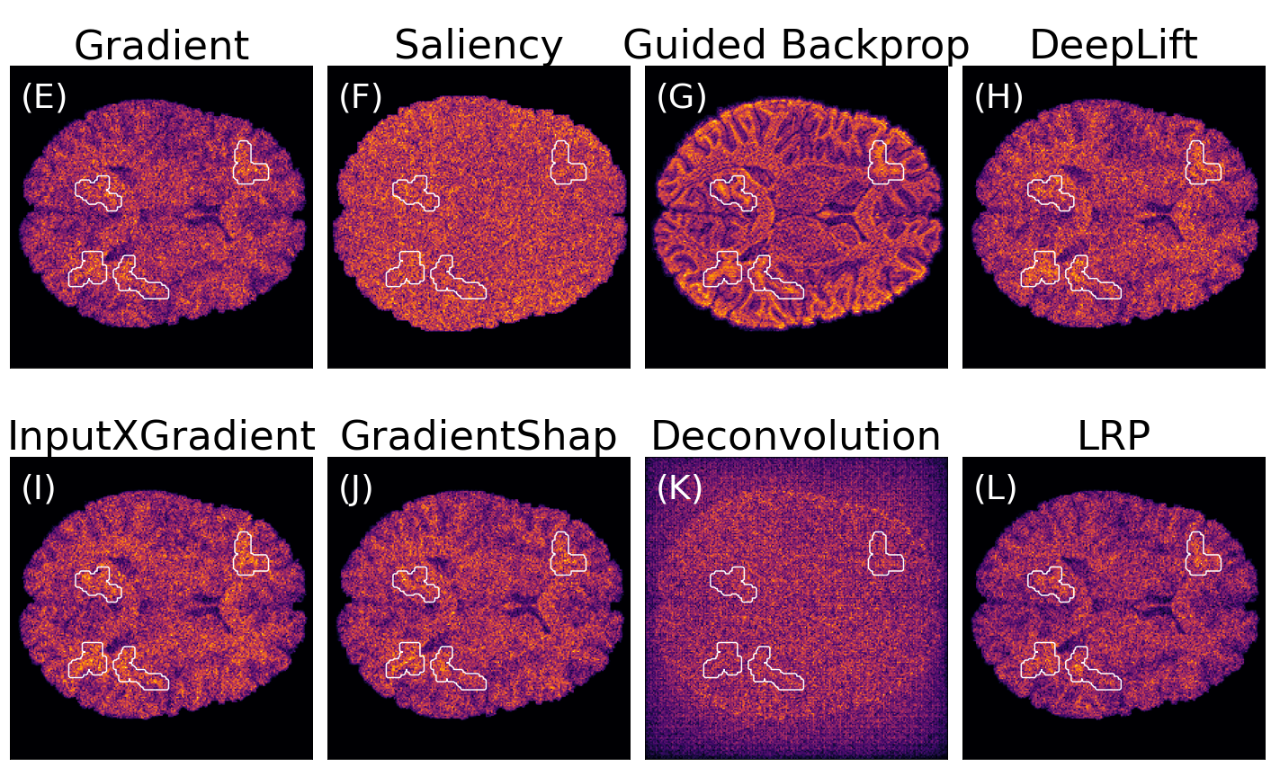
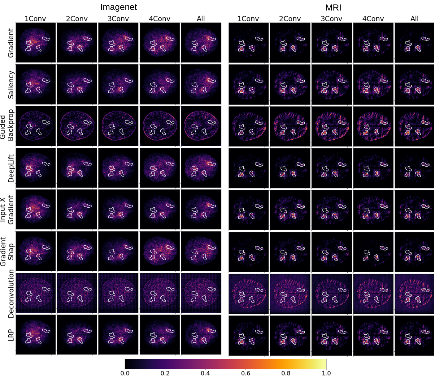
Figure 3 displays importance heat maps for a test sample with four irregular lesions. These explanations are obtained by eight XAI methods for five degrees of fine-tuning. Plots are divided into two sections reflecting the two corpora used for pre-training (ImageNet and MRI female vs. male). The white contours in each heat map represent the ground-truth of the explanation. A good explanation should give high attribution to regions inside the white contour and low everywhere else. In this respect, most of the explanations appear to perform well, identifying most of the lesions, especially for high degrees of fine-tuning. However, the explanations generally do not highlight all of the lesions in the ground-truth. This image also shows that, for some XAI methods, the explanation may deteriorate for an intermediate degree of fine-tuning, and then improve again. This can be seen especially in the results of the model pre-trained with ImageNet data. Heat maps of the untrained baseline model are shown in the section F of the supplement.
When comparing the ‘explanations’ obtained from models pre-trained on ImageNet data with the ones from models pre-trained on MRI data, the latter seems to contain less contamination from the structural features of the MRI background, especially for Deconvolution and Guided Backpropagation. We can further argue that some models seem to do a better job identifying the lesions than others. Particularly noisy explanations are obtained with Deconvolution, especially for models pre-trained with ImageNet data. In this case, pixels with higher importance attribution seem to form a regular grid, roughly covering the shape of the brain of the underlying MRI slice. For models pre-trained on the MRI corpus, Deconvolution is able to place higher importance within the lesions for higher degrees of fine-tuning.
4.2 Quantitative analysis of explanation performance
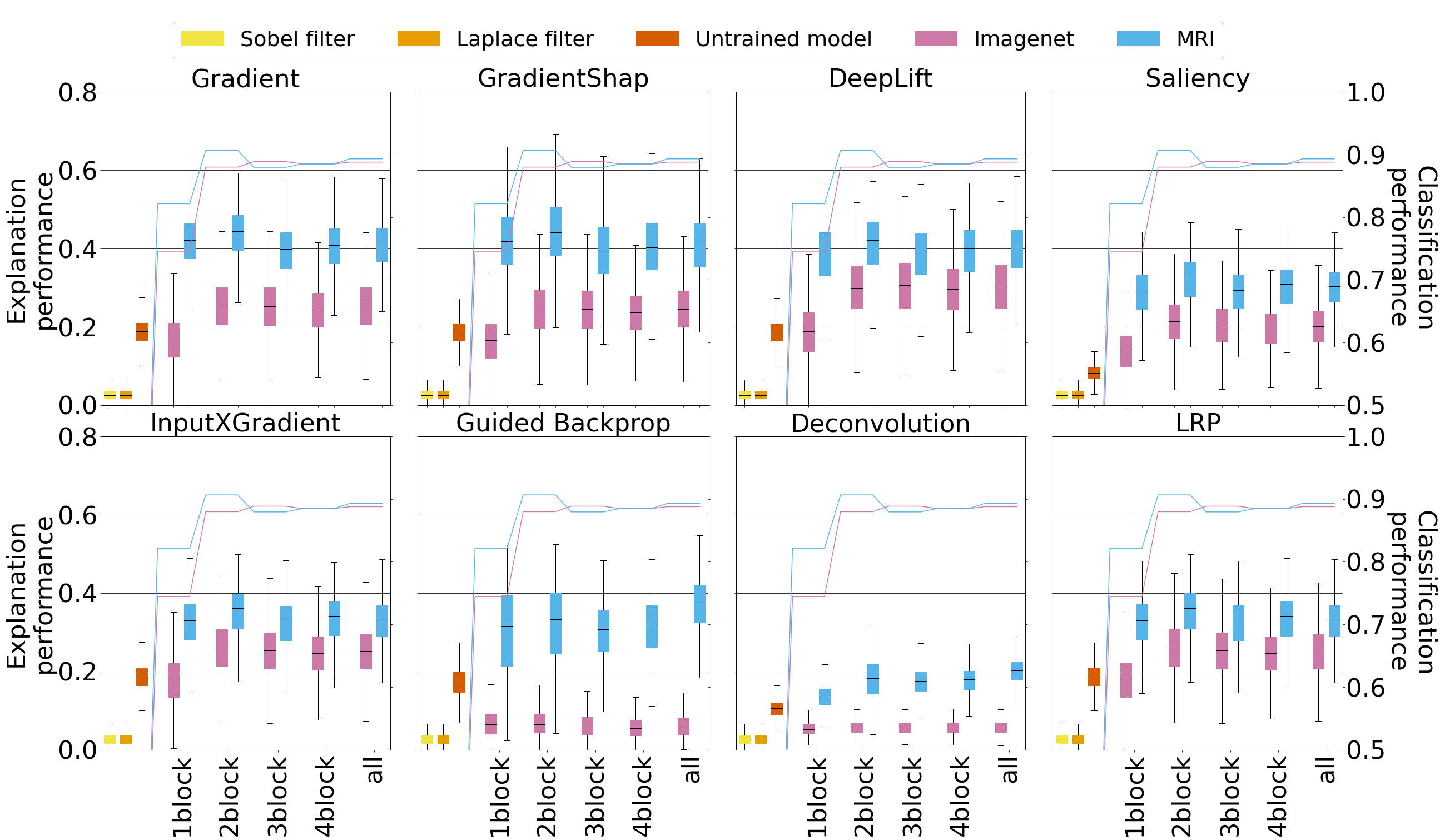
Figure 4 shows quantitative explanation performance. Here, each boxplot was derived from the intersection of test images that were correctly classified by all models (). The results obtained for the edge filter baseline as well as the random baseline model are derived from the same images. Note that the edge detection filters only depend on the given image and are independent of models and XAI methods. Thus, identical results are presented for edge filters in each subfigure. The lines in the background correspond to the average classification performance (test accuracy) of the five models for each degree of fine-tuning. The random baseline model is only one and has a test accuracy of . Interestingly, models pre-trained with ImageNet data consistently achieved higher classification performance than models pre-trained with MR images. The classification performance of the models pre-trained with MR images peaks at an intermediate degree of fine-tuning (3conv), while the models pre-trained with ImageNet improve with higher fine-tuning degrees.
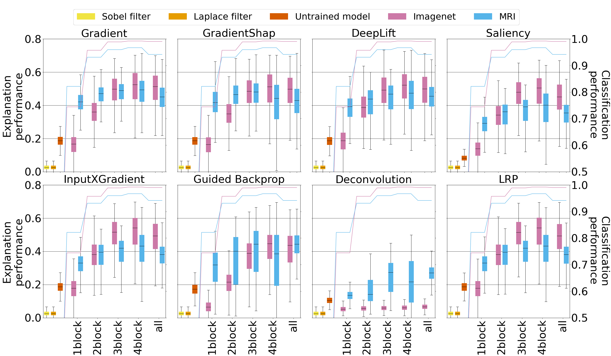
In some settings, ImageNet pre-training leads to considerably worse explanation performance. This is the case for specific methods such as Deconvolution and, to some extent, Guided Backpropagation. Moreover ImageNet pre-training leads to worse explanations across all XAI methods for lower degrees of fine-tuning (1conv and 2conv), where large parts of the models are prohibited to depart from the internal representations learned on the ImageNet data.
As a function of the amount of fine-tuning, explanation performance generally increases with higher degrees of fine-tuning. However, depending on the XAI method used, and the corpus used for pre-training, this trend plateaus or even slightly reverses at a high degree of fine-tuning (4conv).
Importantly, explanation performance appears to strongly correlate with the classification performance of the underlying model. As classification accuracy could represent a potential confound to our analysis, we repeated our quantitative analysis of explanation performance based on five models with similar classification performance per pre-training corpus and degree of fine-tuning. Here, it is apparent that, when controlling for classification performance, models pre-trained on MRI data consistently outperform equally well-predicting models that were pre-trained on ImageNet data in terms of explanation performance. These results are presented in supplementary in section G.
5 Discussion
The field of XAI has produced a plethora of methods whose goal it is to ‘explain’ predictions performed by deep learning and other complex models, including CNNs. However, quantitative evaluations of these methods based on ground-truth data are scarce. Even if these methods are based on seemingly intuitive principles, XAI can only serve its purpose if it is itself properly validated, which is so far not often done. The present study was designed to create a benchmark within which explanation quality can be objectively quantified. To this end, we designed a well-defined ground-truth dataset for model explanations, where we modelled artificial data to resemble the important clinical use case of structural MR image classification for the diagnosis of brain lesions. With this benchmark dataset, we propose a framework to evaluate the influence of pre-training on explanation performance.
We observed a correlation between classification accuracy and explanation performance, which could be expected since a more accurate model is likely to more successfully focus on relevant input features. Networks trained on ImageNet data may have learned representations for objects occurring only outside the domain of brain images (e.g., cats and dogs). The existence of such representations in the network seems to negatively affect XAI methods, whose importance maps are in parts derived by propagating network activations backwards through the network. Consistent with this remark is the observation that for lower degrees of fine-tuning (1conv and 2conv), the explanation quality of models pre-trained with ImageNet data is worse compared to models pre-trained with MR images. These findings challenge the popular view that the low-level information captured by the first layers of a CNN can be shared across domains.
Our quantitative analysis suggests a large dispersion of explanation performance for all XAI methods, which may be unexpected given the controlled setting in which these methods have been applied here. Individual explanations can range from very good to very poor even for high overall classification accuracy, indicating a high risk of misinterpretation for a considerable fraction of inputs.
Limitations
Note, our analysis of XAI methods is limited to one DNN architecture, VGG-16, mainly showcasing the utility of our devised ground-truth dataset for model explanations. Furthermore, the lesion generation process resembles the idea of white matter hyperintensities where we aim to approximate specific neurodegenerative disorders from a ‘model perspective’, where a natural prediction task would be ‘healthy’ vs. ‘lesioned brain’. But it would be difficult to define a ground-truth for the class ‘healthy’. Hence, we chose to create a classification problem based on two different shapes of lesions: round vs elongated. Admittedly, this distinction has no immediate physiological basis and serves purely the purpose of this benchmark, i.e., we can solve a classification task well enough by using a model architecture considered popular in this field. In this work, we are leveraging the HCP data as background for our prediction task. Since we recently learned that HCP will not permit us to publish derivative work ourselves, we plan to replace HCP MR images with equivalent ones from the IXI dataset111https://brain-development.org/ixi-dataset, made available under the Creative Common license. While we are unable to implement the change now, we plan to make the complete dataset available under a similar licence by the time of the conference. We expect neither substantial qualitative nor quantitative changes in the results and discussions provided in this work, given the equivalence of the two datasets.
We argue that the quantitative validation of the correctness of XAI methods is still a greatly under-investigated topic given how popular some of the methods have become. Major efforts both on the theoretical and empirical side are needed to create a framework within which evidence for the correctness of such methods can be provided. As a first step towards such a goal, meaningful definitions of what actually constitutes a correct explanation need to be devised. While in our study, ground-truth explanations were defined through a data generation process, other definitions, depending on the intended use of the XAI, are conceivable. The existence of such definitions would then pave the way for a theoretical analysis of XAI methods as well as for use-case-dependent empirical validations.
6 Conclusion
In this work we created a versatile synthetic image dataset that allows us to quantitatively study the classification and explanation performances of CNN and similar complex ML methods in a highly controlled yet realistic setting, resembling a clinical diagnosis/anomaly detection task based on medical imaging data. Concretely, we overlaid structural brain MRI data with synthetic lesions representing clinically relevant white matter hyperintensities. We propose this dataset, to evaluate the explanations obtained from pre-trained models. Our study is set apart from the majority of work on XAI in that it uses a well-defined ground-truth for explanations, which allows us to quantitatively evaluate the ‘explanation’ performance of several XAI methods.
Our study revealed a strong correlation between the classification performance of the model and the explanation performance of the XAI methods. Despite this correlation, models fine-tuned to a greater extent were shown to lead to better explanations. Controlling for classification performance, models pre-trained on MRI data lead to better explanations for every XAI method. The explanation performance of models pre-trained on within-domain images seem to have more stable explanation performance for a bigger range of classification accuracies. On the other hand, the explanation performance of models pre-trained with more general images quickly degrades with lower classification performance.
The quantitative analysis of the explanations also shows a concerning variability of explanation performance values, suggesting that, when these methods are used to explain an individual prediction, a large uncertainty is associated with the correctness of the resulting importance map. This is a critical issue when using XAI methods to ‘explain’ predictions in high-stake fields such as medicine.
References
- Agarwal et al. [2022] C. Agarwal, E. Saxena, S. Krishna, M. Pawelczyk, N. Johnson, I. Puri, M. Zitnik, and H. Lakkaraju. Openxai: Towards a transparent evaluation of model explanations. arXiv preprint arXiv:2206.11104, 2022.
- Ardalan and Subbian [2022] Z. Ardalan and V. Subbian. Transfer learning approaches for neuroimaging analysis: A scoping review. Frontiers in Artificial Intelligence, 5, 2022. ISSN 2624-8212. doi: 10.3389/frai.2022.780405.
- Arras et al. [2022] L. Arras, A. Osman, and W. Samek. Clevr-xai: A benchmark dataset for the ground truth evaluation of neural network explanations. Information Fusion, 81:14–40, 2022. ISSN 1566-2535.
- Bach et al. [2015a] S. Bach, A. Binder, G. Montavon, F. Klauschen, K.-R. Müller, and W. Samek. On pixel-wise explanations for non-linear classifier decisions by layer-wise relevance propagation. PLOS ONE, 10(7):1–46, 07 2015a. doi: 10.1371/journal.pone.0130140.
- Bach et al. [2015b] S. Bach, A. Binder, G. Montavon, F. Klauschen, K.-R. Müller, and W. Samek. On pixel-wise explanations for non-linear classifier decisions by layer-wise relevance propagation. PLOS ONE, 10(7):1–46, 07 2015b.
- Cheng and Malhi [2017] P. M. Cheng and H. S. Malhi. Transfer learning with convolutional neural networks for classification of abdominal ultrasound images. J Digit Imaging, 30(2):234–243, Apr. 2017.
- Cherti and Jitsev [2021] M. Cherti and J. Jitsev. Effect of Pre-Training Scale on Intra- and Inter-Domain Full and Few-Shot Transfer Learning for Natural and Medical X-Ray Chest Images. pages 1–6. Medical Imaging Meets NeurIPS (MedNeurIPS), Sydney / online (Australia), 6 Dec 2021 - 14 Dec 2021, 2021.
- Dar et al. [2020] S. U. H. Dar, M. Özbey, A. B. Çatlı, and T. Çukur. A transfer-learning approach for accelerated MRI using deep neural networks. Magnetic Resonance in Medicine, 84(2):663–685, 2020. doi: 10.1002/mrm.28148.
- Das and Rad [2020] A. Das and P. Rad. Opportunities and challenges in explainable artificial intelligence (XAI): A survey, 2020.
- Deng et al. [2009a] J. Deng, W. Dong, R. Socher, L.-J. Li, K. Li, and L. Fei-Fei. Imagenet: A large-scale hierarchical image database. In 2009 IEEE Conference on Computer Vision and Pattern Recognition, pages 248–255, 2009a.
- Deng et al. [2009b] J. Deng, W. Dong, R. Socher, L.-J. Li, K. Li, and L. Fei-Fei. Imagenet: A large-scale hierarchical image database. In 2009 IEEE conference on computer vision and pattern recognition, pages 248–255. Ieee, 2009b.
- d’Arbeloff et al. [2019] T. d’Arbeloff, M. L. Elliott, A. R. Knodt, T. R. Melzer, R. Keenan, D. Ireland, S. Ramrakha, R. Poulton, T. Anderson, A. Caspi, T. E. Moffitt, and A. R. Hariri. White matter hyperintensities are common in midlife and already associated with cognitive decline. Brain Communications, 1(1), 12 2019. ISSN 2632-1297. doi: 10.1093/braincomms/fcz041.
- Elam et al. [2021] J. S. Elam, M. F. Glasser, M. P. Harms, S. N. Sotiropoulos, J. L. Andersson, G. C. Burgess, S. W. Curtiss, R. Oostenveld, L. J. Larson-Prior, J.-M. Schoffelen, M. R. Hodge, E. A. Cler, D. M. Marcus, D. M. Barch, E. Yacoub, S. M. Smith, K. Ugurbil, and D. C. Van Essen. The human connectome project: A retrospective. NeuroImage, 244:118543, 2021.
- European Commission [2018] European Commission. 2018 Reform of EU Data Protection Rules, 2018. URL {https://ec.europa.eu/commission/sites/beta-political/files/data-protection-factsheet-changes_en.pdf}.
- Fischl [2012] B. Fischl. FreeSurfer. NeuroImage, 62(2):774–781, 2012. ISSN 1053-8119. doi: 10.1016/j.neuroimage.2012.01.021.
- Gebru et al. [2021] T. Gebru, J. Morgenstern, B. Vecchione, J. W. Vaughan, H. Wallach, H. D. Iii, and K. Crawford. Datasheets for datasets. Communications of the ACM, 64(12):86–92, 2021.
- Gevaert et al. [2022] A. Gevaert, A.-J. Rousseau, T. Becker, D. Valkenborg, T. De Bie, and Y. Saeys. Evaluating Feature Attribution Methods in the Image Domain. arXiv e-prints, art. arXiv:2202.12270, 2022.
- Glasser et al. [2013] M. F. Glasser, S. N. Sotiropoulos, J. A. Wilson, T. S. Coalson, B. Fischl, J. L. Andersson, J. Xu, S. Jbabdi, M. Webster, J. R. Polimeni, D. C. Van Essen, and M. Jenkinson. The minimal preprocessing pipelines for the human connectome project. NeuroImage, 80:105–124, 2013. ISSN 1053-8119. doi: 10.1016/j.neuroimage.2013.04.127.
- Haufe et al. [2014] S. Haufe, F. Meinecke, K. Görgen, S. Dähne, J.-D. Haynes, B. Blankertz, and F. Bießmann. On the interpretation of weight vectors of linear models in multivariate neuroimaging. NeuroImage, 87:96–110, 2014.
- Hofmann et al. [2022] S. M. Hofmann, F. Beyer, S. Lapuschkin, O. Goltermann, M. Loeffler, K.-R. Müller, A. Villringer, W. Samek, and A. V. Witte. Towards the interpretability of deep learning models for multi-modal neuroimaging: Finding structural changes of the ageing brain. NeuroImage, 261:119504, 2022.
- Jenkinson et al. [2002] M. Jenkinson, P. Bannister, M. Brady, and S. Smith. Improved optimization for the robust and accurate linear registration and motion correction of brain images. NeuroImage, 17(2):825–841, 2002. ISSN 1053-8119. doi: 10.1006/nimg.2002.1132.
- Jenkinson et al. [2012] M. Jenkinson, C. F. Beckmann, T. E. Behrens, M. W. Woolrich, and S. M. Smith. FSL. NeuroImage, 62(2):782–790, 2012. ISSN 1053-8119. doi: 10.1016/j.neuroimage.2011.09.015.
- Krizhevsky et al. [2012] A. Krizhevsky, I. Sutskever, and G. E. Hinton. ImageNet Classification with Deep Convolutional Neural Networks. In F. Pereira, C. J. C. Burges, L. Bottou, and K. Q. Weinberger, editors, Advances in Neural Information Processing Systems 25, pages 1097–1105. Curran Associates, Inc., 2012.
- Lundberg and Lee [2017] S. Lundberg and S.-I. Lee. A unified approach to interpreting model predictions, 2017.
- Milchenko and Marcus [2013] M. Milchenko and D. Marcus. Obscuring surface anatomy in volumetric imaging data. Neuroinformatics, 11(1):65–75, Jan 2013. ISSN 1559-0089. doi: 10.1007/s12021-012-9160-3.
- Otsu [1979] N. Otsu. A threshold selection method from gray-level histograms. IEEE Transactions on Systems, Man, and Cybernetics, 9(1):62–66, 1979. doi: 10.1109/TSMC.1979.4310076.
- Pan and Yang [2010] S. J. Pan and Q. Yang. A survey on transfer learning. IEEE Transactions on Knowledge and Data Engineering, 22(10):1345–1359, 2010. doi: 10.1109/TKDE.2009.191.
- Pineau et al. [2021] J. Pineau, P. Vincent-Lamarre, K. Sinha, V. Larivière, A. Beygelzimer, F. d’Alché Buc, E. Fox, and H. Larochelle. Improving reproducibility in machine learning research (a report from the neurips 2019 reproducibility program). The Journal of Machine Learning Research, 22(1):7459–7478, 2021.
- Schmidt et al. [2012] P. Schmidt, C. Gaser, M. Arsic, D. Buck, A. Förschler, A. Berthele, M. Hoshi, R. Ilg, V. J. Schmid, C. Zimmer, et al. An automated tool for detection of flair-hyperintense white-matter lesions in multiple sclerosis. Neuroimage, 59(4):3774–3783, 2012.
- Shirokikh et al. [2020] B. Shirokikh, I. Zakazov, A. Chernyavskiy, I. Fedulova, and M. Belyaev. First U-Net layers contain more domain specific information than the last ones. In S. Albarqouni, S. Bakas, K. Kamnitsas, M. J. Cardoso, B. Landman, W. Li, F. Milletari, N. Rieke, H. Roth, D. Xu, and Z. Xu, editors, Domain Adaptation and Representation Transfer, and Distributed and Collaborative Learning, pages 117–126, Cham, 2020. Springer International Publishing. ISBN 978-3-030-60548-3.
- Shrikumar et al. [2017] A. Shrikumar, P. Greenside, and A. Kundaje. Learning important features through propagating activation differences. 2017. doi: 10.48550/ARXIV.1704.02685.
- Simonyan and Zisserman [2014] K. Simonyan and A. Zisserman. Very deep convolutional networks for large-scale image recognition. arXiv, 2014. doi: 10.48550/ARXIV.1409.1556.
- Simonyan et al. [2013] K. Simonyan, A. Vedaldi, and A. Zisserman. Deep inside convolutional networks: Visualising image classification models and saliency maps, 2013.
- Springenberg et al. [2015] J. Springenberg, A. Dosovitskiy, T. Brox, and M. Riedmiller. Striving for simplicity: The all convolutional net. In ICLR (workshop track), 2015.
- Sundararajan et al. [2017] M. Sundararajan, A. Taly, and Q. Yan. Axiomatic attribution for deep networks, 2017.
- Tjoa and Guan [2020] E. Tjoa and C. Guan. Quantifying Explainability of Saliency Methods in Deep Neural Networks. 2020.
- Topol [2019] E. J. Topol. High-performance medicine: the convergence of human and artificial intelligence. Nature Medicine, 25(1):44–56, Jan 2019. ISSN 1546-170X. doi: 10.1038/s41591-018-0300-7.
- Valverde et al. [2021] J. M. Valverde, V. Imani, A. Abdollahzadeh, R. De Feo, M. Prakash, R. Ciszek, and J. Tohka. Transfer learning in magnetic resonance brain imaging: A systematic review. Journal of Imaging, 7(4), 2021. ISSN 2313-433X. doi: 10.3390/jimaging7040066.
- Van Essen et al. [2013] D. C. Van Essen, S. M. Smith, D. M. Barch, T. E. Behrens, E. Yacoub, and K. Ugurbil. The WU-Minn human connectome project: An overview. NeuroImage, 80:62–79, 2013. ISSN 1053-8119. doi: 10.1016/j.neuroimage.2013.05.041.
- Wharton et al. [2015] S. B. Wharton, J. E. Simpson, C. Brayne, and P. G. Ince. Age-associated white matter lesions: The MRC cognitive function and ageing study. Brain Pathology, 25(1):35–43, 2015. doi: 10.1111/bpa.12219.
- Wilming et al. [2022] R. Wilming, C. Budding, K.-R. Müller, and S. Haufe. Scrutinizing XAI using linear ground-truth data with suppressor variables. Machine Learning, 2022.
- Zeiler and Fergus [2014] M. D. Zeiler and R. Fergus. Visualizing and understanding convolutional networks. In D. Fleet, T. Pajdla, B. Schiele, and T. Tuytelaars, editors, Computer Vision – ECCV 2014, pages 818–833, Cham, 2014. Springer International Publishing. ISBN 978-3-319-10590-1.
- Zhou et al. [2022] Y. Zhou, S. Booth, M. T. Ribeiro, and J. Shah. Do feature attribution methods correctly attribute features? In Proceedings of the AAAI Conference on Artificial Intelligence, volume 36, pages 9623–9633, 2022.
- Zucco et al. [2018] C. Zucco, H. Liang, G. D. Fatta, and M. Cannataro. Explainable sentiment analysis with applications in medicine. In 2018 IEEE International Conference on Bioinformatics and Biomedicine (BIBM), pages 1740–1747, 2018. doi: 10.1109/BIBM.2018.8621359.
Checklist
-
1.
For all authors…
-
(a)
Do the main claims made in the abstract and introduction accurately reflect the paper’s contributions and scope? [Yes]
-
(b)
Did you describe the limitations of your work? [Yes]
-
(c)
Did you discuss any potential negative societal impacts of your work? [Yes] see supplementary material section "Societal Impact"
-
(d)
Have you read the ethics review guidelines and ensured that your paper conforms to them? [Yes]
-
(a)
-
2.
If you are including theoretical results…
-
(a)
Did you state the full set of assumptions of all theoretical results? [N/A]
-
(b)
Did you include complete proofs of all theoretical results? [N/A]
-
(a)
-
3.
If you ran experiments (e.g. for benchmarks)…
-
(a)
Did you include the code, data, and instructions needed to reproduce the main experimental results (either in the supplemental material or as a URL)? [Yes] see supplemental material section "Code and Data Access"
-
(b)
Did you specify all the training details (e.g., data splits, hyperparameters, how they were chosen)? [Yes]
-
(c)
Did you report error bars (e.g., with respect to the random seed after running experiments multiple times)? [Yes]
-
(d)
Did you include the total amount of compute and the type of resources used (e.g., type of GPUs, internal cluster, or cloud provider)? [Yes]
-
(a)
-
4.
If you are using existing assets (e.g., code, data, models) or curating/releasing new assets…
-
(a)
If your work uses existing assets, did you cite the creators? [Yes]
-
(b)
Did you mention the license of the assets? [Yes]
-
(c)
Did you include any new assets either in the supplemental material or as a URL? [Yes]
-
(d)
Did you discuss whether and how consent was obtained from people whose data you’re using/curating? [Yes] see Datasheet
-
(e)
Did you discuss whether the data you are using/curating contains personally identifiable information or offensive content? [Yes] see Datasheet
-
(a)
-
5.
If you used crowdsourcing or conducted research with human subjects…
-
(a)
Did you include the full text of instructions given to participants and screenshots, if applicable? [N/A]
-
(b)
Did you describe any potential participant risks, with links to Institutional Review Board (IRB) approvals, if applicable? [N/A]
-
(c)
Did you include the estimated hourly wage paid to participants and the total amount spent on participant compensation? [N/A]
-
(a)
Appendix
Appendix A Human Connectome Project and IXI
Data were provided in part by the Human Connectome Project (HCP), WU-Minn Consortium (Principal Investigators: David Van Essen and Kamil Ugurbil; 1U54MH091657) funded by the 16 NIH Institutes and Centers that support the NIH Blueprint for Neuroscience Research; and by the McDonnell Center for Systems Neuroscience at Washington University. For more information, see the datasheet in section L.
As described in the discussion of the main text, we are aiming to replace the HCP data with the IXI222https://brain-development.org/ixi-dataset data, which comes with a Creative Commons license enabling us to fully publish our dataset under the same license.
Appendix B Code and Data Access
The code generating the lesion maps and performing the model training as well as running the explanation methods is available on Github: https://github.com/Marta54/Pretrain_XAI_gt . Please, find the generated lesion data under this link: The lesions are generated using the function create_lesion() from the Finetuning_on_2500_images.ipynb notebook.
Appendix C Steps to create lesions.
Figure 5 displays the different steps, from the noise image to the final lesion needed to create the lesions to be added to the MRI background. These steps are thoroughly described in section 2.1 of the main body of this paper.
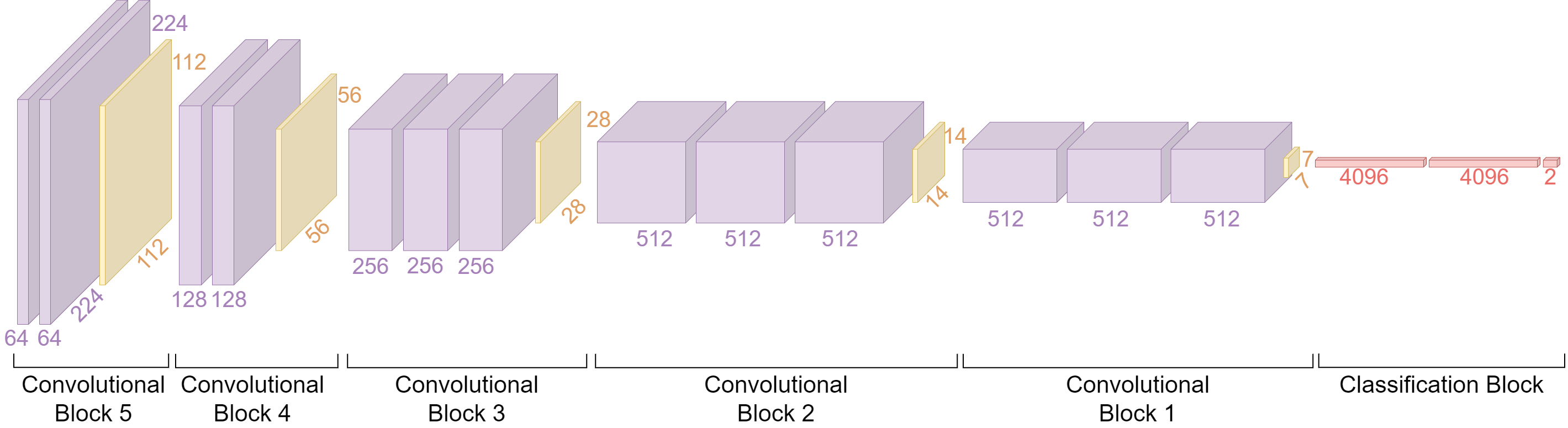
Appendix D VGG-16 architecture
Figure 6 shows the different layers that build VGG-16 architecture. The purple layers represent convolutional layers, the yellow layers represent max-pooling layers, and the red layers represent fully-connected layers. In this architecture, max-pooling layers separate the NN into blocks of convolutional layers. These are the blocks used to identify five different degrees of fine-tuning.
To fine-tune the pre-trained model we used the holdout and validation datasets from the HCP. The data used to fine-tune the model consists of 2500 slices from the holdout dataset. This was done because the training dataset from the HCP had been already used to pre-train the model, which could create dependencies if the same data was used as the background of the fine-tuning dataset. Another 2500 slices from the same holdout dataset, were used to obtain the quantitative explanation performance. Lastly, 2500 slices from the validation dataset were used to validate the fine-tuning.
Appendix E Model training
To train and fine-tune the models, we used an internal cluster equipped with GPUs of the type NVIDIA GeForce GTX 1080 Ti.
Appendix F Baselines of XAI methods
Figure 7 displays the heat maps obtained by applying the XAI methods to a model randomly initialised and untrained. Here we can see that some methods (Gradient, DeepLift, GradientShap, InputXGradient, Guided Backpropagation and LRP) seem to give a higher attribution in the pixels inside the ground-truth than to the rest of the pixels. For those methods, some lighter regions of the brain, such as the grey matter, also have higher attribution than the rest of the brain. Thus, we can suppose that the lesions are highlighted in these methods because their pixels have higher intensity in the input image, making them more salient than other brain regions. Saliency and Deconvolution have a more homogeneous attribution distribution and do not highlight the lesions.
Appendix G Models fine-tuned with similar performance
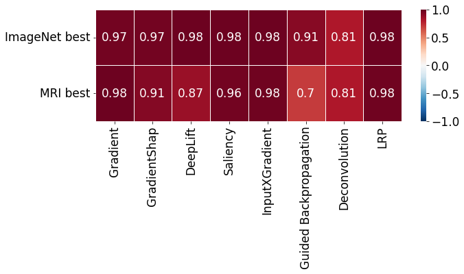
Figure 8 shows Pearson correlations between the average explanation accuracy of individual XAI methods and the test classification accuracy achieved by the underlying model for every combination of data used for pre-training and XAI methods. For almost all combinations, very strong positive correlations 0.9 can be observed, representing a potential confound for the analysis of explanation performance as a function of the degree of model fine-tuning. Therefore, we control for unequal classification accuracy by selecting five models per fine-tuning degree that achieve similar test accuracy, close to 90%. The classification performance of these models is presented in Table 1. The models selected with this criterion for the lowest degree of fine-tuning (1conv) are unchanged, as these models do not reach the specified performance. The classification performance of the selected models for larger degrees of fine-tuning is between 88% and 89%.
| 1conv | 2conv | 3conv | 4conv | all | ||
|---|---|---|---|---|---|---|
| LR | 0.020 | 0.008 | 0.008 | 0.008 | 0.004 | |
| 75.00% | 89.10% | 89.70% | 89.00% | 89.40% | ||
| ImageNet | Test Acc | 74.90% | 88.10% | 89.60% | 89.10% | 89.40% |
| 74.80% | 88.80% | 88.90% | 88.20% | 89.00% | ||
| mean | 74.90% | 88.67% | 89.40% | 88.77% | 89.27% | |
| LR | 0.038 | 0.030 | 0.015 | 0.030 | 0.010 | |
| 82.80% | 90.50% | 86.70% | 88.20% | 88.20% | ||
| MRI | Test Acc | 79.50% | 89.60% | 89.20% | 87.40% | 90.50% |
| 79.60% | 89.20% | 87.60% | 88.80% | 89.60% | ||
| mean | 80.63% | 89.77% | 87.83% | 88.13% | 89.43% |
Figure 9 is analogous to Figure 3 but is based on models that achieved comparable classification accuracy across fine-tuning degrees. Compared to Figure 3, importance maps obtained for models that were pre-trained on ImageNet data appear to be degraded, while corresponding maps obtained for models that were pre-trained on MR images still closely resemble those obtained for best performing models as depicted in Figure 3.
Figure 10 shows corresponding quantitative results for models that achieved comparable performance across fine-tuning degrees. The attained explanation performance of models that were pre-trained with MR images is similar to the explanation performance obtained with the best performing models as depicted in Figure 4. The same is not true for models pre-trained with ImageNet data. Even though these models still achieve high classification accuracies of almost 90%, explanations derived from the resulting models seem to be much worse than for the best performing models (which achieve accuracies close to 100%). Importantly, for comparable classification accuracy, models pre-trained on ImageNet data were also consistently achieved lower explanation performance than models pre-trained on MR images. Overall, explanations obtained from models pre-trained with images from a similar domain may have a similar quality throughout a bigger range of classification performance values compared to explanations obtained from models pre-trained with images from different domains. In other words, this would indicate that using within-domain images to pre-train models can be beneficial with respect to the interpretability of a model even if the resulting models achieves lower classification performance.
Appendix H Societal Impact
Our work mainly contributes to the evaluation of XAI methods, to avoid potential negative consequences of using such methods in high-stake decision environments, which we see as outweighing potential negative societal impact by a large margin. On the other hand, we propose one specific and narrow definition of feature importance and to that extent ‘define’ how XAI methods ‘should’ work. It is conceivable that this could lead to potential rejections of future ideas or approaches that might be able to generate superior explanations apart from the concept employed in this work.
Appendix I Concerns of former reviewers
Former reviewers were mainly concerned about the lack of employing a variety of machine learning models for comparing explanation results. Here we stress, that, rather than conducting an exhaustive study of the behaviour of popular XAI methods in relation to specific model architectures, with our work, we aim to predominantly contribute to the evaluation of XAI methods by providing a controlled ground-truth dataset, with known explanations, class-related features, enabling future research to benchmark new XAI methods. Also, the dataset itself was criticised by former reviewers as not resembling a real-world medical problem, and it was suggested that we use annotated data with real lesions. We emphasize that expert annotations do not constitute a stable ground-truth, and that full knowledge about the underlying ground-truth is needed to validate methods, a purpose that is only served be synthetically crafted data. In the medical domain, ML methods are often used with the expectation that they will uncover statistical relations that are either unknown or too complex (e.g. involving non-linear interactions of features) for human experts to discern. When experts annotate data, they may inadvertently overlook these features, potentially leading to false-positive detections if an XAI method indeed succeeds in highlighting them. Conversely, human experts may provide annotations that are simply incorrect. They can be influenced by pseudo-correlations in the data resulting from limited sample size in prior studies, or mistakenly base their judgement on confounders or even suppressors. In such instances, a correctly functioning XAI method may be mistakenly accused of delivering false-negative detections. Note in this context that clinical doctrines are highly fluctuating as new evidence is constantly being produced. For example, the assumed causal role of beta-amyloid and tau protein plaques in the brain for various types of dementia is currently being challenged. To address these challenges and strive towards real-world validity, experiments involving annotated real data are valuable and complementary next steps. However, they cannot entirely replace ground-truth experiments involving synthetic or manipulated real data due to their intrinsic biases. And generating realistic artificial and controllable image data for the MRI domain is, in itself, a very hard problem. Here, we simulate lesions that resemble so-called white-matter hyperintensities in MR images, which have been linked to ageing-related cognitive decline. At the same time, we acknowledge that our classification problem (round vs. elongated lesions) is not overly realistic. However, we provide a classification scenario where the background, real brain slice images, provides features that are partially leveraged by ML models, which put XAI methods in the position to differentiate between class-related features, artificial lesions, and realistic brain-related features. Where we think that this distinction constitutes a realistic environment for XAI methods. In this light, our dataset can be seen as a first instance of contributing to the performance quantification of explanations produced by XAI methods for the MRI domain.
Appendix J IXI Dataset
As part of the project “IXI – Information eXtraction from Images (EPSRC GR/S21533/02)”333https://brain-development.org/ixi-dataset/, 600 MR images from normal, healthy subjects were collected. The data was made available under the Creative Commons CC BY-SA 3.0 license.
Appendix K The ML Paper Reproducibility Checklist (as per [28], v2.0)
-
1.
For all models and algorithms presented, check if you include:
-
(a)
A clear description of the mathematical setting, algorithm, and/or model. [Yes]
-
(b)
A clear explanation of any assumptions. [Yes]
-
(c)
An analysis of the complexity (time, space, sample size) of any algorithm [Yes]
-
(a)
-
2.
For any theoretical claim, check if you include:
-
(a)
A clear statement of the claim. [N/A]
-
(b)
A complete proof of the claim. [N/A]
-
(a)
-
3.
For all datasets used, check if you include:
-
(a)
The relevant statistics, such as number of examples. [Yes]
-
(b)
The details of train / validation / test splits. [Yes]
-
(c)
An explanation of any data that were excluded, and all pre-processing step [Yes]
-
(d)
A link to a downloadable version of the dataset or simulation environment [Yes]
-
(e)
For new data collected, a complete description of the data collection process, such as instructions to annotators and methods for quality control [Yes]
-
(a)
-
4.
For all shared code related to this work, check if you include:
-
(a)
Specification of dependencies. [Yes]
-
(b)
Training code. [Yes]
-
(c)
Evaluation code. [Yes]
-
(d)
(Pre-)trained model(s). [Yes]
-
(e)
README file includes table of results accompanied by precise command to run to produce those results [Yes]
-
(a)
-
5.
For all reported experimental results, check if you include:
-
(a)
The range of hyper-parameters considered, method to select the best hyper-parameter configuration, and specification of all hyper-parameters used to generate results. [Yes]
-
(b)
The exact number of training and evaluation runs [Yes]
-
(c)
A clear definition of the specific measure or statistics used to report results. [Yes]
-
(d)
A description of results with central tendency (e.g. mean) and variation (e.g. error bars). [Yes]
-
(e)
The average runtime for each result, or estimated energy cost. [Yes]
-
(f)
A description of the computing infrastructure used. [Yes]
-
(a)
Appendix L Datasheet (template by [16])
Motivation
For what purpose was the dataset created? Was there a specific task in mind? Was there a specific gap that needed to be filled? Please provide a description.
With the rise of deep neural networks (DNNs) and their deployment in high-stake decision environments, many researchers and developers ask for techniques that shed light on the inner workings of such complex models, as they are commonly perceived as opaque ‘black-box’ models. Thus, XAI methods were developed to approach this problem. However, the lack of clarity on what formal problem the field of XAI is supposed to solve led to a branch of research to quantitatively validate such methods. Along this line of research, we propose a dataset where class-relevant features are known by construction and can serve as ground-truth explanations.
A common practice of applying ML models for the medical domain, here MRI, where labelled data are scarce, because of the cumbersome and expensive acquisition process, is, to deploy transfer learning techniques. The main purpose of the provided dataset is therefore to provide a validation framework, for novel XAI approaches aiming to explain decision made by pre-trained ML models that are fine-tuned to solve a specific MRI classification task.
Who created this dataset (e.g., which team, research group) and on behalf of which entity (e.g., company, institution, organization)?
This dataset has been constructed by the research group "Quality AI Labs" at the Technische Universität Berlin444https://www.tu.berlin/uniml. Furthermore, the ‘base’ dataset, the background images, was provided by the Human Connectome Project.
Who funded the creation of the dataset? If there is an associated grant, please provide the name of the grantor and the grant name and number.
Data were provided in part by the Human Connectome Project, WU-Minn Consortium (Principal Investigators: David Van Essen and Kamil Ugurbil; 1U54MH091657) funded by the 16 NIH Institutes and Centers that support the NIH Blueprint for Neuroscience Research; and by the McDonnell Center for Systems Neuroscience at Washington University.
This result is part of a project that has received funding from the European Research Council (ERC) under the European Union’s Horizon 2020 research and innovation programme (Grant agreement No. 758985), the German Federal Ministry for Economy and Climate Action (BMWK) in the frame of the QI-Digital Initiative, and the Heidenhain Foundation.
Composition
What do the instances that comprise the dataset represent (e.g., documents, photos, people, countries)? Are there multiple types of instances (e.g., movies, users, and ratings; people and interactions between them; nodes and edges)? Please provide a description.
This dataset only contains brain images with artificial lesions. Ground-truth explanations come in the form of lesion maps represented as images as well.
How many instances are there in total (of each type, if appropriate)?
Our dataset consists of a training, validation and holdout dataset that encompasses 2500 images each. For the underlying HCP data, we chose 601 subjects for training, 206 for validation, and 201 for holdout. From these subjects, we generated 24924 slices for the training dataset, 8539 slices for the validation dataset, and 8319 slices for the holdout dataset. Where the holdout set and 2500 images from the validation set combined represent our provided lesion dataset. The training dataset consists of 24924 slices and is used for model pre-training and takes , the validation dataset and the holdout set .
Does the dataset contain all possible instances or is it a sample (not necessarily random) of instances from a larger set? If the dataset is a sample, then what is the larger set? Is the sample representative of the larger set (e.g., geographic coverage)? If so, please describe how this representativeness was validated/verified. If it is not representative of the larger set, please describe why not (e.g., to cover a more diverse range of instances, because instances were withheld or unavailable).
For the creation of the dataset, we leveraged all subjects contained in the HCP data.
What data does each instance consist of? “Raw” data (e.g., unprocessed text or images) or features? In either case, please provide a description.
Each instance consists of a list [image,gender,age] where the image is a grayscale MRI slice, gender is a binary variable with for male and for female, and age is a binary variable as well, and takes the value for the subjects age and otherwise.
Is there a label or target associated with each instance? If so, please provide a description.
We assign labels according to the shape of the artificial lesions incorporated into the brain images. For images comprising round lesions we assign the label , and for images comprising irregular lesions we assign the label .
Is any information missing from individual instances? If so, please provide a description, explaining why this information is missing (e.g., because it was unavailable). This does not include intentionally removed information, but might include, e.g., redacted text.
No.
Are relationships between individual instances made explicit (e.g., users’ movie ratings, social network links)? If so, please describe how these relationships are made explicit.
The Open Access HCP dataset does not contain any relational information.
Are there recommended data splits (e.g., training, development/validation, testing)? If so, please provide a description of these splits, explaining the rationale behind them.
We already provide a standard data split: training/validation and holdout (testing) set.
Are there any errors, sources of noise, or redundancies in the dataset? If so, please provide a description.
The HCP dataset consists of real-world MRI slices that are naturally suffering from recording artefacts and potential pre-processing perturbations.
Is the dataset self-contained, or does it link to or otherwise rely on external resources (e.g., websites, tweets, other datasets)? If it links to or relies on external resources, a) are there guarantees that they will exist, and remain constant, over time; b) are there official archival versions of the complete dataset (i.e., including the external resources as they existed at the time the dataset was created); c) are there any restrictions (e.g., licenses, fees) associated with any of the external resources that might apply to a future user? Please provide descriptions of all external resources and any restrictions associated with them, as well as links or other access points, as appropriate.
Newer versions of this dataset, which are not planned so far, will rely on the HCP, or possibly on the IXI datasets, as well. Apart from that, our dataset is self-contained.
Does the dataset contain data that might be considered confidential (e.g., data that is protected by legal privilege or by doctor-patient confidentiality, data that includes the content of individuals non-public communications)? If so, please provide a description.
Our dataset contains brain slices of individuals, though names and other meta-data that can identify individuals are not contained, also the MRI records are de-faced and considered de-identified under HIPAA [13].
Does the dataset contain data that, if viewed directly, might be offensive, insulting, threatening, or might otherwise cause anxiety? If so, please describe why.
No.
Does the dataset relate to people? If not, you may skip the remaining questions in this section.
Yes.
Does the dataset identify any subpopulations (e.g., by age, gender)? If so, please describe how these subpopulations are identified and provide a description of their respective distributions within the dataset.
The provided training dataset consists of slices of male brain images, the validation dataset consists of slices of male brain images, and the holdout dataset consists of slices of male brain images.
Is it possible to identify individuals (i.e., one or more natural persons), either directly or indirectly (i.e., in combination with other data) from the dataset? If so, please describe how.
Even though the dataset only consists of brain image slices and binary sex and age variables, it is possible to identify individuals.
Does the dataset contain data that might be considered sensitive in any way (e.g., data that reveals racial or ethnic origins, sexual orientations, religious beliefs, political opinions or union memberships, or locations; financial or health data; biometric or genetic data; forms of government identification, such as social security numbers; criminal history)? If so, please provide a description.
No.
Collection Process
How was the data associated with each instance acquired? Was the data directly observable (e.g., raw text, movie ratings), reported by subjects (e.g., survey responses), or indirectly inferred/derived from other data (e.g., part-of-speech tags, model-based guesses for age or language)? If data was reported by subjects or indirectly inferred/derived from other data, was the data validated/verified? If so, please describe how.
The brain slices or images, were extracted from MRI recordings acquired via MRI devices by the HCP project (for more details see [39]). Otherwise, the lesions were artificially generated (see section 2.1 of the main text).
What mechanisms or procedures were used to collect the data (e.g., hardware apparatus or sensor, manual human curation, software program, software API)? How were these mechanisms or procedures validated?
We created lesions algorithmically. For the details of the recording mechanisms of the MRI recordings, consult the corresponding publication of the HCP project [39].
If the dataset is a sample from a larger set, what was the sampling strategy (e.g., deterministic, probabilistic with specific sampling probabilities)?
The brain slice images were randomly sampled from a larger dataset. The corresponding seeds are made available via our Github repository: https://github.com/Marta54/Pretrain_XAI_gt.
Who was involved in the data collection process (e.g., students, crowdworkers, contractors) and how were they compensated (e.g., how much were crowdworkers paid)?
No data were collected from our lab members, but for the HCP project, it is not apparent who was involved in the data collection process (see [39]).
Over what timeframe was the data collected? Does this timeframe match the creation timeframe of the data associated with the instances (e.g., recent crawl of old news articles)? If not, please describe the timeframe in which the data associated with the instances was created.
A timeline for the HCP project is provided by Elam et al. [13].
Were any ethical review processes conducted (e.g., by an institutional review board)? If so, please provide a description of these review processes, including the outcomes, as well as a link or other access point to any supporting documentation.
Yes, see Van Essen et al. [39], Elam et al. [13]. However, here we only use de-identified data with respect to HIPAA.
Does the dataset relate to people? If not, you may skip the remaining questions in this section.
Yes.
Did you collect the data from the individuals in question directly, or obtain it via third parties or other sources (e.g., websites)?
The HCP project [39] is a third-party project that provides access to high-quality brain imaging data, which we based our dataset on.
Were the individuals in question notified about the data collection? If so, please describe (or show with screenshots or other information) how notice was provided, and provide a link or other access point to, or otherwise reproduce, the exact language of the notification itself.
Participants explicitly expressed consent to participate in the HCP project [39].
Did the individuals in question consent to the collection and use of their data? If so, please describe (or show with screenshots or other information) how consent was requested and provided, and provide a link or other access point to, or otherwise reproduce, the exact language to which the individuals consented.
For the HCP data, the informed consent document explicitly states that the data of the participants will be shared publicly over the internet [13].
If consent was obtained, were the consenting individuals provided with a mechanism to revoke their consent in the future or for certain uses? If so, please provide a description, as well as a link or other access point to the mechanism (if appropriate).
Individuals provided informed consent with the knowledge that their data will be distributed via the internet. As the data use terms [39] allows for the re-distribution of derivative work under the same license, even if a participant withdraws their informed consent, deleting their data completely is potentially infeasible.
Has an analysis of the potential impact of the dataset and its use on data subjects (e.g., a data protection impact analysis) been conducted? If so, please provide a description of this analysis, including the outcomes, as well as a link or other access point to any supporting documentation.
For the HCP data, privacy concerns were discussed leading to two tiers of data access: "Open Access Data" and "Restricted Access Data" [13]. We use the Open Access dataset.
Preprocessing/cleaning/labeling
Was any preprocessing/cleaning/labeling of the data done (e.g., discretization or bucketing, tokenization, part-of-speech tagging, SIFT feature extraction, removal of instances, processing of missing values)? If so, please provide a description. If not, you may skip the remainder of the questions in this section.
Yes. From the initial HCP data, we selected only slices with less than 55% black pixels. From these, their intensity was changed so that every slice had a similar average pixel intensity. These slices were also reshaped from pixels to . The HCP images used were also previously pre-processed with FreeSurfer 5.1 software and registered to MNI152 space using FSL’s linear FLIRT tool, followed by FNIRT algorithm as described in [39]. The HCP data was also defaced using the technique described in [25].
Was the “raw” data saved in addition to the preprocessed/cleaned/labeled data (e.g., to support unanticipated future uses)? If so, please provide a link or other access point to the “raw” data.
We saved the image slices selected from the HCP dataset that we used. These images are available on our provided Dropbox repository and are contained in the folder named Pre-training dataset.
The raw data of our dataset consists of the slices, gender and age corresponding to those slices and the slices were used both to pre-train the model and to serve as a background to our synthetic lesions. Note that the slices used to pre-train a model to the task of classifying female and male slices were not the same slices used to fine-tune the model, as we only used the holdout set and parts of the validation set.
Is the software used to preprocess/clean/label the instances available? If so, please provide a link or other access point.
Yes. The pre-processing of our dataset can be found in https://github.com/Marta54/Pretrain_XAI_gt, while the pre-process made to the HCP data can be followed from the HCP paper [39].
Uses
Has the dataset been used for any tasks already? If so, please provide a description.
Our dataset has not been used for other tasks yet. The HCP dataset is a widely used research dataset [13].
Is there a repository that links to any or all papers or systems that use the dataset? If so, please provide a link or other access point.
An aggregated overview of published papers using the HCP dataset can be found in Elam et al. [13]. The HCP website itself provides a list of selected publications using the HCP dataset: https://www.humanconnectome.org/study/hcp-young-adult/publications
What (other) tasks could the dataset be used for?
The data we provide is dedicated to analyzing XAI methods applied to pre-trained models that are fine-tuned on our dataset. Technically, one could employ this dataset to perform benchmarks for model fine-tuning on the MRI domain.
Is there anything about the composition of the dataset or the way it was collected and preprocessed/cleaned/labeled that might impact future uses? For example, is there anything that a future user might need to know to avoid uses that could result in unfair treatment of individuals or groups (e.g., stereotyping, quality of service issues) or other undesirable harms (e.g., financial harms, legal risks) If so, please provide a description. Is there anything a future user could do to mitigate these undesirable harms?
For our provided pre-training dataset we were aiming to balance the sampled brain slides according to the subjects’ sex. For reasoning of the composition of the HCP dataset we refer to Van Essen et al. [39].
Are there tasks for which the dataset should not be used? If so, please provide a description.
Yes, according to the data access terms of the HCP project, it is prohibited to try to establish the identity of the included human subjects (e.g. see [39]).
Distribution
Will the dataset be distributed to third parties outside of the entity (e.g., company, institution, organization) on behalf of which the dataset was created? If so, please provide a description.
Yes. We aim to make our dataset publically available under a Creative Commons license. Note, currently we aim to replace the HPC dataset by the publically accessible IXI dataset.
How will the dataset will be distributed (e.g., tarball on website, API, GitHub) Does the dataset have a digital object identifier (DOI)?
We plan to host a general benchmark suite for XAI methods to evaluate the quality of produced explanations. In the realm of that benchmark suite, we aim to offer our MRI dataset as well, which will be hosted at the Physikalisch-Technische Bundesanstalt in Germany.
When will the dataset be distributed?
Currently, the MRI dataset is only available for the reviewers but we plan to provide a publically accessible dataset, preferably hosted via the Physikalisch-Technische Bundesanstalt in Germany, made available by publication of this manuscript.
Will the dataset be distributed under a copyright or other intellectual property (IP) license, and/or under applicable terms of use (ToU)? If so, please describe this license and/or ToU, and provide a link or other access point to, or otherwise reproduce, any relevant licensing terms or ToU, as well as any fees associated with these restrictions.
We would like to publish our dataset under a Creative Commons license.
Have any third parties imposed IP-based or other restrictions on the data associated with the instances? If so, please describe these restrictions, and provide a link or other access point to, or otherwise reproduce, any relevant licensing terms, as well as any fees associated with these restrictions.
The HCP dataset requires the agreement of the license provided by the HCP project555https://www.humanconnectome.org/study/hcp-young-adult/document/wu-minn-hcp-consortium-open-access-data-use-terms .
Do any export controls or other regulatory restrictions apply to the dataset or to individual instances? If so, please describe these restrictions, and provide a link or other access point to, or otherwise reproduce, any supporting documentation.
The Open Access HCP dataset is de-identified and the project’s data access terms apply.
Maintenance
Who will be supporting/hosting/maintaining the dataset?
The dataset is supported by the authors and by the QAI Labs research group. Currently, the dataset is temporarily hosted on Dropbox for the review process. It is planned to host the dataset on servers of the German governance institute the “Physikalisch-Technische Bundesanstalt”, to ensure long-time availability. If reviewers have concrete concerns about this hosting strategy, the usage of the “Open Science Framework” (OSF666osf.io) can be an alternative hosting service.
How can the owner/curator/manager of the dataset be contacted (e.g., email address)?
The authors of this dataset can be reached at the e-mail address: haufe@tu-berlin.de.
Is there an erratum? If so, please provide a link or other access point.
If errors are found an erratum will be added to the website containing all meta-information about this dataset.
Will the dataset be updated (e.g., to correct labeling errors, add new instances, delete instances)? If so, please describe how often, by whom, and how updates will be communicated to users (e.g., mailing list, GitHub)?
As we plan the dataset as part of an XAI benchmark suite hosted at the Physikalisch-Technische Bundesanstalt in Germany, updates and error corrections will be part of the maintenance of this benchmark platform, i.e. a changelog can be provided via the corresponding website.
If the dataset relates to people, are there applicable limits on the retention of the data associated with the instances (e.g., were individuals in question told that their data would be retained for a fixed period of time and then deleted)? If so, please describe these limits and explain how they will be enforced.
Participants of the HCP project had to sign an informed consent form, which explicitly states that their data will be made public via the Internet, thus its access is not constrained by any limits other than the data use terms777https://www.humanconnectome.org/study/hcp-young-adult/document/wu-minn-hcp-consortium-open-access-data-use-terms.
Will older versions of the dataset continue to be supported/hosted/maintained? If so, please describe how. If not, please describe how its obsolescence will be communicated to users.
Older versions of this dataset could be hosted via the website of the aforementioned XAI benchmark.
If others want to extend/augment/build on/contribute to the dataset, is there a mechanism for them to do so? If so, please provide a description. Will these contributions be validated/verified? If so, please describe how. If not, why not? Is there a process for communicating/distributing these contributions to other users? If so, please provide a description.
As mentioned above, we aim to publish this dataset under a Creative Commons license, which yields an opportunity for other researchers to freely access this dataset and create derivative work.