The Multimode Character of Quantum States Released from a Superconducting Cavity

Abstract

Quantum state transfer by propagating wave packets of electromagnetic radiation requires tunable couplings between the sending and receiving quantum systems and the propagation channel or waveguide. The highest fidelity of state transfer in experimental demonstrations so far has been in superconducting circuits. Here, the tunability always comes together with nonlinear interactions, arising from the same Josephson junctions that enable the tunability. The resulting non-linear dynamics correlates the photon number and spatio-temporal degrees of freedom and leads to a multi-mode output state, for any multi-photon state. In this work, we study as a generic example the release of complex quantum states from a superconducting resonator, employing a flux tunable coupler to engineer and control the release process. We quantify the multi-mode character of the output state and discuss how to optimize the fidelity of a quantum state transfer process with this in mind.

I Introduction

The exchange of quantum states between distant locations is an important ingredient in secure communication networks and in scalable architectures for quantum computing kimble2008quantum ; wehner2018quantum . Quantum bits encoded in the higher dimensional oscillator modes of superconducting cavities have been demonstrated to withstand photon losses and permit elementary error correction vlastakis2013deterministically ; leghtas2015confining ; ofek2016extending ; campagne2020quantum ; puri2020bias ; ni2023beating . It would be desirable to use such multiphoton quantum states also for quantum communication purposes grimsmo2020quantum ; PhysRevA.106.042614 .

While a linear mapping between a single oscillator mode and the continuum of propagating field modes, in principle, transfers the quantum state of the former to a traveling single-mode pulse, the temporal control of the release process is not trivial. In superconducting circuits, tunable couplers based on Josephson junctions are employed to control the evolution and release process in different architectures, such as fixed-frequency transmons, flux tunable transmons, or tunable transmission line resonators houck2007generating ; pierre2014storage ; PhysRevX.4.041010 ; PhysRevA.93.063823 ; PhysRevApplied.8.054015 ; pfaff2017controlled ; axline2018demand ; cozzolino2019high ; burkhart2021error ; yang2023deterministic . While the non-linearity of the Josephson junction enables tunable coupling, it also adds effective self-Kerr and cross-Kerr terms to the oscillator Hamiltonian. These non-linear terms may entangle the spatio-temporal release with the photon number contents of the pulse, and thus the emission becomes multi-mode in character and it may not function properly in a quantum network.

In this article, we present a general analysis that takes the multi-mode character of the emission process fully into account. We employ a master equation approach that readily incorporates both the coherent coupling to the output field and decay and decoherence channels, and we use the quantum regression theorem to assess the mode decomposition of the emitted radiation.

For the more quantitative discussion, we consider superconducting circuits. With low loss rates and strong coupling, these are promising platforms to efficiently prepare and emit quantum states into propagating modes krantz2019quantum ; blais2021circuit . Different studies and experiments have been done with a low number of photons yin2013catch ; pechal2014microwave . In this paper, we theoretically analyze an experimentally relevant superconducting circuit architecture for which we can control the out-coupling strength and compute the accompanying non-linear couplings. The propagation transfer and the recapture of the field by downstream circuit components can then be analyzed by the method presented in kiilerich2019input .

The article is structured as follows: In Sec. II, we provide the formalism determining the characteristics of the output field of the quantum system. In Sec. III, we describe the superconducting emitter and tunable out-coupler in detail, and in Sec. IV we provide numerical results and study the quantitative effects of the nonlinearity on the multi-mode character of different bosonic quantum states released from the circuit. Finally, we summarize the paper in Sec. VI.

II Multimode Theory

Figure 1: Time-dependent spectra of the output field from a non-linear (a) and a linear (b) resonator. Panel (a) shows the radiation from a non-linear resonator with constant frequency $\omega_{0}$, outcoupling rate $1/\kappa=1\,\mu s$, and Kerr coefficient $\chi/2\pi=.47$ MHz prepared in an initial Fock state $\ket{n}=\ket{5}$. The insert in panel (a) shows that the emitted radiation occupies several eigenmodes. In panels (b) we assume a vanishing Kerr coefficient $\chi=0$ and a time-dependent oscillator frequency $\omega(t)=\omega_{0}+$max$(0,2\chi(n\exp(-\kappa t)-1))$. As shown in the inset of panel (b), the output field is a single-mode Fock state with $n=5$.

In this section, we consider a single nonlinear resonator as a toy model for a non-linear emitter with the Hamiltonian

$$H_{S}(t)=\omega(t)a^{\dagger}a+\chi(t)a^{\dagger 2}a^{2},$$ (1)

having time-dependent frequency $\omega(t)$ and self-Kerr coefficient $\chi(t)$, using angular frequency units of energy ($\hbar=1$). If we assume the emitter is coupled to a waveguide with constant strength $\sqrt{\kappa}$, the evolution of the reduced density matrix $\varrho(t)$ of the resonator is described by the Lindblad master equation with a single Lindblad operator $\sqrt{\kappa}$, describing the dissipation to the waveguide,

$$\frac{\partial\varrho(t)}{\partial t}=-i[H_{S}(t),\varrho(t)]+\kappa\Bigg{(}a\varrho(t)a^{\dagger}-\frac{1}{2}[a^{\dagger}a,\varrho(t)]\Bigg{)}.$$ (2)

To find the mode decomposition of the emitted field one can utilize its first-order autocorrelation function

$$\mathcal{G}^{(1)}(t_{1},t_{2})=\kappa\langle a^{\dagger}(t_{2})a(t_{1})\rangle=\sum_{i}n_{i}v^{*}_{i}(t_{1})v_{i}(t_{2}),$$ (3)

which can be expressed in terms of the orthonormal output modes $v_{i}(t)$, with the mean photon number $n_{i}$. The autocorrelation function $\mathcal{G}^{(1)}(t_{1},t_{2})$ can be calculated using the quantum regression theorem breuer2002theory ; gardiner2004quantum

$$\mathcal{G}^{(1)}(t_{1},t_{2})=\kappa\mathrm{Tr}\Bigg{[}a^{\dagger}\mathcal{L}(t_{2},t_{1})[a\mathcal{L}(t_{1},0)\varrho_{s}(0)]\Bigg{]},$$ (4)

where $\mathcal{L}(t^{\prime},t)$ represents the linear time evolution map of the master equation (2) from time $t$ to $t^{\prime}$. The time-dependent spectrum related to the autocorrelation function in Eq. (4) is found by the Fourier transform

$$\mathcal{I}(\omega,t)=\int_{-\infty}^{+\infty}\mathrm{d}s\,\,\,\,\mathcal{G}^{(1)}\bigg{(}t+\frac{s}{2},t-\frac{s}{2}\bigg{)}\,\,e^{-i\omega s},$$ (5)

which provides information about the time-dependent frequency content of the output field.

Output field spectra for a nonlinear resonator and a linear resonator are shown in Fig. 1, where in both cases the resonator is initialized in the Fock state $\ket{\psi}=\ket{5}$. For the parameters in the figure caption, the time-dependent spectrums show the emission of a wide range of frequencies for both linear and non-linear resonators. The spectrum in Fig. 1 (a), shows a visible gap between the frequency pertaining to each emitted photon, proportional to the amount of the Kerr nonlinearity $2\chi$. The insert shows that multiple output field modes are populated in the field emitted by the nonlinear resonator.

For comparison, in Fig. 1(b), we assume a linear resonator, $\chi=0$, with a time-dependent frequency $\omega(t)$ chosen to give a similar frequency range of the emitted field as in (a). The insert in panel (b) shows that the output field in this case only occupies a single (chirped) mode. In the next section, we model a realistic quantum emitter implemented in superconducting circuits and we assess how the non-linear elements used for tuning the emission process affect the mode character and purity of the emitted quantum state.

III Physical Model

Several approaches have been used to map a stationary resonator mode to a propagating pulse mode. To optimally control the release of a quantum state, we consider the storage system (cavity), initiated in the desired quantum state $|\psi\rangle$, described by the creation and annihilation operators $a^{\dagger},a$ and frequency $\omega_{a}$. The storage cavity is dispersively coupled to a flux-tunable transmon tinkham2004introduction ; PhysRevA.76.042319 ; blais2021circuit ; rasmussen2021superconducting described by the operators $c^{\dagger},c$ and frequency $\omega_{c}$, through the coupling strength $g_{ac}\ll(\omega_{c}-\omega_{a})$. In addition to the storage cavity, the coupler is also dispersively coupled to a leakage cavity, described by frequency $\omega_{b}$ and operators $b^{\dagger},b$, with the coupling $g_{bc}\ll(\omega_{b}-\omega_{c})$; see Fig. 2.

Figure 2: Schematic of the emitter. The non-linear coupler interacts with both the storage and the leakage cavity. By driving the coupler at the frequency $\omega^{a}_{01}-\omega^{b}_{01}$, it implements a frequency conversion and resonant transfer of quanta between the storage and leakage cavity, as governed by a beam splitter interaction $H_{bs}(t)$ between the two cavities at frequencies $\omega^{a}_{01}$ and $\omega^{b}_{01}$. Due to the nonlinearity of the coupler, the beam splitter interaction is accompanied by self-Kerr and cross-Kerr non-linear interactions; see Eq. (III), which leads to an output field populating several mode´s $v_{1}(t),v_{2}(t),v_{3}(t),...$ .

The entire system is described by the effective Hamiltonian

$$H_{S}(t)= \omega_{a}a^{\dagger}a+\omega_{b}b^{\dagger}b+\omega_{c}c^{\dagger}c$$

$$+2E_{J}\bigg{[}\cos(\frac{\varphi_{\mathrm{ext}}(t)}{2})-\cos(\frac{\varphi_{\mathrm{dc}}}{2})\bigg{]}\frac{\varphi^{2}_{c}}{2}$$

$$-2E_{J}\cos(\frac{\varphi_{\mathrm{ext}}(t)}{2})\frac{\varphi^{4}_{c}}{4!},$$ (6)

where $\varphi_{c}$ and $E_{J}$ correspond to the reduced flux operator of the transmon and the energy of the junction, respectively. The AC flux drive on the coupler is $\varphi_{\mathrm{ext}}(t)=\varphi_{\mathrm{dc}}+F(t)\sin(\omega_{d}t)$ which is described by the time-dependent amplitude $F(t)\equiv\delta\tanh{(t/t_{0})}\ll 1$ and frequency $\omega_{d}$, where $\delta$ and $t_{0}$ correspond to the amplitude and rate of turning on the drive, respectively. For more details on the derivation of the Hamiltonian (III) see Appendix A.

In the dispersive regime, the reduced flux of the coupler is found as the superposition of all dressed modes nigg2012black ; marcos2013superconducting

$$\varphi_{c}= \frac{2\pi}{\phi_{0}}\phi_{c},$$

$$\phi_{c}= \frac{\lambda_{a}(a+a^{\dagger})+\lambda_{b}(b+b^{\dagger})+\lambda_{c}(c+c^{\dagger})}{\sqrt{2}}\equiv\frac{A+A^{\dagger}}{\sqrt{2}},$$ (7)

where $\phi_{c}$ is the flux of the coupler and the coefficients $\lambda_{a,b,c}$ are described in Eq. (A.2). Using the Taylor expansion (A.1), we insert Eq. (III) in the Hamiltonian (III), thus the second line of Eq. (III) is obtained as

$$H^{l}(t)=\frac{-2E_{J}\pi^{2}}{\phi_{0}^{2}}\Bigg{[} \frac{\sin(\frac{\varphi_{\mathrm{dc}}}{2})F(t)\sin(\omega_{d}t)}{2}$$

$$+\frac{\cos(\frac{\varphi_{\mathrm{dc}}}{2})}{8}F(t)^{2}\sin(\omega_{d}t)^{2}\Bigg{]}(2A^{\dagger}A+\bar{\lambda}),$$ (8)

where $\bar{\lambda}=[A,A^{\dagger}]$. The third line of Eq. (III) (fourth order of the flux operator), provides the nonlinear interactions as follows

$$H_{nl}\approx \frac{-\pi^{4}E_{J}\cos(\frac{\varphi_{\mathrm{ext}}(t)}{2})}{3\phi_{0}^{4}}\Bigg{[}12\bar{\lambda}A^{\dagger}A+6A^{\dagger}A^{\dagger}AA\Bigg{]},$$ (9)

where we just keep the terms conserving the energy.

We assume that the coupler is initiated in the ground state and mediates the resonant frequency conversion without itself being excited. This permits the elimination of its quantum degrees of freedom at all times. If we consider $\omega_{d}=\omega_{b}-\omega_{a}$ and utilize the rotating wave approximation and transform to the rotating frame interaction picture with respect to $\omega_{a}a^{\dagger}a+\omega_{b}b^{\dagger}b+\omega_{c}c^{\dagger}c$, the Hamiltonian is obtained as

$$H_{S}(t)= S_{a}(t)a^{\dagger}a+S_{b}(t)b^{\dagger}b+\chi_{a}a^{2\dagger}a^{2}+\chi_{b}b^{2\dagger}b^{2}$$

$$+\chi_{ab}a^{\dagger}ab^{\dagger}b-ig_{\mathrm{swap}}(t)(b^{\dagger}a-a^{\dagger}b),$$ (10)

where the parameters are as follows

$$\chi_{a(b)}= \frac{-2\pi^{4}E_{J}\cos(\frac{\varphi_{\mathrm{dc}}}{2})}{\phi_{0}^{4}}\lambda_{a(b)}^{4},$$

$$\chi_{ab}= \frac{-8\pi^{4}E_{J}\cos(\frac{\varphi_{\mathrm{dc}}}{2})}{\phi_{0}^{4}}\lambda_{a}^{2}\lambda_{b}^{2},$$

$$g_{\mathrm{swap}}(t)= (\frac{\pi^{2}}{\phi_{0}^{2}}-\frac{\bar{\lambda}\pi^{4}}{\phi_{0}^{4}})E_{J}\sin(\frac{\varphi_{dc}}{2})\lambda_{a}\lambda_{b}F(t),$$

$$S_{a(b)}(t)= (\frac{\bar{\lambda}\pi^{4}}{\phi_{0}^{4}}-\frac{\pi^{2}}{\phi_{0}^{2}})\frac{E_{J}\cos(\frac{\varphi_{\mathrm{dc}}}{2})\lambda_{a(b)}^{2}}{4}F(t)^{2},$$ (11)

and $S_{a(b)}(t)$ are the Stark shifts induced by the flux drive. The dressed mode coefficients $\lambda_{a(b)}$ in Eq. (III,III) are proportional to the ratio $\lambda_{a(b)}\propto g_{a(b),c}/\Delta_{a(b),c}$, where $g_{a(b),c}$ and $\Delta_{a(b),c}$ correspond to the coupling strength and detuning between the coupler and the storage (leakage) cavity. The coupler is coupled to the storage (leakage) cavities through the coupling capacitance $C_{ac}(C_{bc})$ where by changing the capacitance strengths, different values of the conversion rates $g_{\mathrm{swap}}$ and also nonlinear terms $\chi_{ab},\chi_{a(b)}$ will be obtained; see Fig. 3. As shown in Fig. 3, the reduction (increase) of the non-linearities $\chi_{a(b)}\propto\lambda_{a(b)}^{4}$ yields a similar effect on the swap rate $g_{\mathrm{swap}}(t)\propto\lambda_{a}\lambda_{b}$, as mentioned $\lambda_{a(b)}\propto g_{a(b),c}\propto C_{a(b)c}$. It is worth noting that while a stronger amplitude of the drive $F(t)$, accelerates the transfer and release process, in this regime the Hamiltonian of the system acquires higher-order nonlinear interactions.

The leakage cavity decays to the waveguide with a constant decay rate $\kappa$. The analysis of the emitted radiation is equivalent to the one presented for the toy model in Sec. II, with the master equation,

$$\frac{\partial\varrho(t)}{\partial t}=-i[H_{S}(t),\varrho(t)]+\kappa\Bigg{(}b\varrho(t)b^{\dagger}-\frac{1}{2}[b^{\dagger}b,\varrho(t)]\Bigg{)},$$ (12)

where $H_{S}(t)$ is given in Eq. (III), and the Lindblad operator $\sqrt{\kappa}b$ describes the dissipation of the leakage cavity to the waveguide. As for the toy model in Eq. (4), the mode decomposition of the first-order correlation function of the field operator $b$, determines the most populated orthonormal output modes.

Figure 3: The change of the nonlinear parameters $\chi_{a},\chi_{ab}$, swap rate $g$, detuning from resonant interaction $\chi_{ab}-2\chi_{a}$, and Purcell rate $4g^{2}/\kappa$ as functions of the value of the coupling capacitance $C_{ac}$, where $1/\kappa=0.2\,\mu s$. The vertical black dashed line corresponds to the parameters used to simulate the lower panels in Fig. 4 and Fig. 5.

Figure 4: The characteristics of the output field for different initial quantum states such as a FS $\ket{n}$, a TCCS (13), and a FCCS (14). The upper panels show (a) the relative occupation of the most populated mode, (c) the state fidelity of the state occupying that mode with respect to the optimal target state, see Eq. (17), and (e) the value of the cat state amplitude $\tilde{\alpha}$ that has the maximum fidelity with the state occupying the most populated mode.The results are shown for the initial FS $\ket{n=3}$ and FCCS and TCCS with amplitude parameter $\alpha=\sqrt{3}$. They are calculated as a function of the non-linear coupling strengths $\chi_{ab}$ and $\chi_{a}$ indicated along the lower and upper axes, which in turn correspond to a varying capacitance between the storage cavity and the coupler in the physical system (see Fig. 3). The self-Kerr $\chi_{b}$ is not specified as the leakage cavity is mostly occupied by the vacuum and the occasional one-photon state. In the lower panels, we assume non-linear interaction parameters $\chi_{ab}/2\pi=$-0.11\text{\,}\mathrm{M}\mathrm{H}\mathrm{z}$$, $\chi_{a}/2\pi=$-0.017\text{\,}\mathrm{M}\mathrm{H}\mathrm{z}$$, and $\chi_{b}/2\pi=$-0.04\text{\,}\mathrm{M}\mathrm{H}\mathrm{z}$$, and we show the same quantities as in the upper panels but for different values of the initial mean photon number $\langle a^{\dagger}a\rangle(t=0)$; see Sec. V for details.

As we saw in Sec. II, non-linear terms in the Hamiltonian cause the output field to populate several temporal field modes of the waveguide. Since the self Kerr and cross Kerr terms $(\chi_{a}a^{2\dagger}a^{2},\chi_{b}b^{2\dagger}b^{2}$ and $\chi_{ab}a^{\dagger}b^{\dagger}ab)$ are inevitable consequences of the tunable coupling in our system, the output field will indeed populate many temporal modes, as will be seen in the next section.

In the limit where $\kappa$ is much larger than the other couplings in the master equation, it is possible to adiabatically eliminate the leakage cavity and obtain an effective Markovian master equation for the storage cavity mode with a Purcell damping rate $\simeq 4g_{\mathrm{swap}}^{2}/\kappa$; green dots in Fig 3. While we do not rely on the quantitative validity of this effective treatment in our numerical studies, we will refer to the value of the Purcell rate in the analysis of the results.

Here, we also note that due to the presence of other dissipation channels, the release process cannot be made arbitrarily slow. Hence, in the experiment, there will be a trade-off between the loss to many less populated modes in the rapid-release regime and to other dissipation channels in the slow-release regime.

IV Release of Fock states and cat states

As illustrated in Sec. II, a linear resonator emits any initial quantum state into a single spatiotemporal mode determined by the time-dependent outcoupling strength. However, the temporal shape of the output field from a nonlinear emitter is correlated with the photon number contents. As discussed in the preceding section, the strength of the coherent swap coupling between the cavities, the effective Purcell decay rate of the storage cavity, and the non-linearity are correlated and vary with the physical parameters of the circuit. In this section, we characterize the output field from the resonator using the variation of the parameters corresponding to the coupling capacitance strength between the storage cavity and the coupler which are shown in 3.

In Fig. 4, we investigate the output field of the emitter for different quantum states such as a Fock state (FS) $\ket{\psi}=\ket{n}$, a two-component cat state (TCCS)

$$\ket{\psi}\propto\ket{\alpha}+\ket{-\alpha}\propto\sum_{n=0}^{\infty}\frac{\alpha^{2n}}{\sqrt{(2n)!}}\ket{2n},$$ (13)

which is a promising candidate for correcting dephasing errors PhysRevA.59.2631 ; PhysRevLett.100.030503 , and a four-component cat state (FCCS)

$$\ket{\psi}\propto\ket{\alpha}+\ket{-\alpha}+\ket{i\alpha}+\ket{-i\alpha}\propto\sum_{n=0}^{\infty}\frac{\alpha^{4n}}{\sqrt{(4n)!}}\ket{4n},$$ (14)

which can be used for quantum storage and communication in the presence of photon loss PhysRevLett.111.120501 ; mirrahimi2014dynamically .

Fig. 4 (a) shows the relative population of the most populated mode $n_{1}/n_{out}$ as a function of the Kerr nonlinearities. The ratio $n_{1}/n_{\mathrm{out}}$ reveals the multimode character of the output field released from a three-photon FS and TCCS and FCCS, composed of coherent states with amplitude $\alpha^{2}=3$. As one expects, the output field becomes more multimode with higher values of nonlinearity and with higher photon numbers. We observe that the FS and the FCCS yield a higher single-mode content than the TCCS with the same photon number. This difference arises partly because the FS and FCCS populate a single, dominant Fock state component, while the TCCS populates both $\ket{n=2}$ and $\ket{n=4}$ components, which are dephased by the Kerr effect and couple to different frequency components of the output field. Panel 4 (b) shows $n_{1}/n_{\mathrm{out}}$ as a function of the initial mean photon number of the storage cavity for the same states using fixed nonlinear parameters, corresponding to the dashed vertical line in Fig. 3. As expected, with a higher number of photons, the resonator non-linearity leads to an output field occupying more modes.

In Fig.4, panel (a), the output field is almost single mode, $n_{1}/n_{\mathrm{out}}\simeq 1$, until $\chi_{ab}/2\pi$ exceeds the value $-0.23$ MHz or equivalently the value $C_{ac}\simeq 4.5$fF in Fig 3. This can be ascribed to the release of photons being meditated by the process, $\ket{n,0}_{a,b}\xrightarrow{\text{swap}}\ket{n-1,1}_{a,b}\xrightarrow[]{\kappa}\ket{n-1,0}_{a,b}$. The energy difference between the states $\ket{n,0}_{a,b},\ket{n-1,1}_{a,b}$ is $\Delta E_{n}=(n-1)(2\chi_{a}-\chi_{ab})$ where a small additional shift is omitted, see Eq. (III). If $\chi_{ab}\simeq 2\chi_{a}$, the transfer is resonant and faster which results in a more single-mode character. According to Fig. 3, the energy difference has a smooth behavior until $C_{ac}\simeq 4.5$fF and hereafter, the transition states rapidly become non-resonant and the slow release in combination with the nonlinearity causes the increasing multimode character, witnessed by the reduction of the population $n_{1}/n_{\mathrm{out}}$ and similar reductions in the other quantifiers of the output field.

V Characterizing the most populated mode

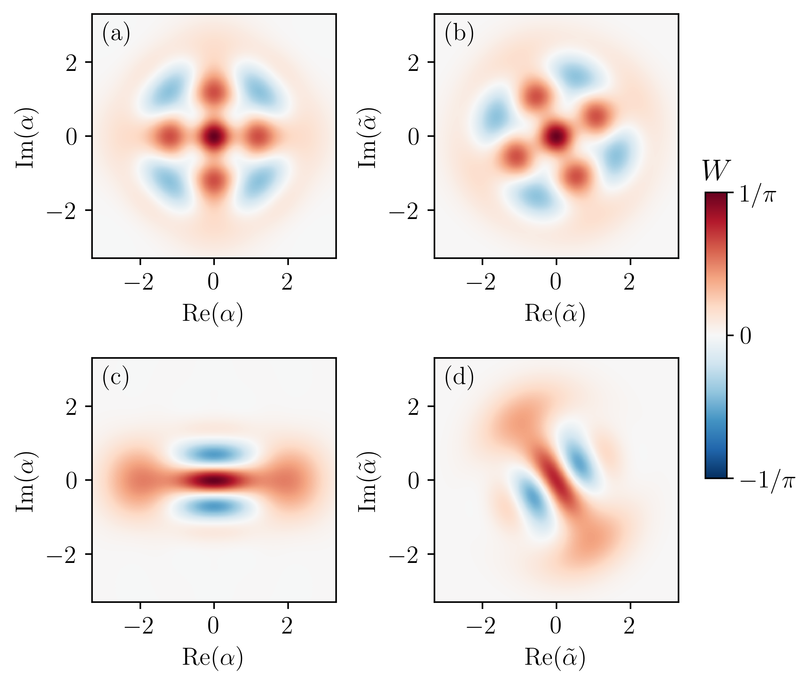
Figure 5: Wigner function of the initial FCCS (a) and the state of the most populated mode of emission (b), the initial TCCS (c) and the corresponding highest fidelity single mode output state (d). The amplitude of the initial cat states is $|\alpha^{2}|=2$ and the nonlinear interactions are $\chi_{ab}/2\pi=-$0.11\text{\,}\mathrm{M}\mathrm{H}\mathrm{z}$,\chi_{a}/2\pi=-$0.017\text{\,}\mathrm{M}\mathrm{H}\mathrm{z}$$, and $\chi_{b}/2\pi=$-0.04\text{\,}\mathrm{M}\mathrm{H}\mathrm{z}$$; the same as panels 4 (b,d,f) . The amplitude of the single mode output cat state for panel (b) is $|\tilde{\alpha}|^{2}=1.96$ with a corresponding fidelity $\mathcal{F}_{\mathrm{4cat}}=.97$. Panel (d) shows the emitted single mode TCCS obtained with the optimal drive rate $t_{0}$ for the flux drive $F(t)=\delta\tanh(t/t_{0})$. This state has a lower amplitude $|\tilde{\alpha}|^{2}=1.66$ and the fidelity $\mathcal{F}_{\mathrm{2cat}}=.85$; See Sec. V.1 for more explanation.

In this section, we address the quantum state contents of the most occupied mode $v_{1}$. This is done by the formalism introduced in kiilerich2019input , which, for the theoretical calculation assumes a downstream ideal linear cavity with mode operators $d,d^{\dagger}$, coupled to the system by the interaction Hamiltonian

$$H_{b,v_{1}}(t)=\frac{i\sqrt{\kappa}}{2}[g_{v_{1}}(t)d^{\dagger}b-g^{*}_{v_{1}}(t)b^{\dagger}d].$$ (15)

The time-dependent coupling between the cavity and waveguide

$$g_{v}(t)=-\frac{v_{1}^{*}(t)}{\sqrt{\int_{0}^{t}\mathrm{d}t^{\prime}|v_{1}(t^{\prime})|^{2}}},$$ (16)

ensures that the cavity captures the contents of the temporal mode $v_{1}(t)$. The dynamics of the cascaded system is described by the Lindblad master equation with total Hamiltonian $H_{T}=H_{S}(t)+H_{b,v_{1}}(t)$ and a single Lindblad operator describes dissipation to the waveguide, $L_{0}(t)=\sqrt{\kappa}b+g_{v_{1}}^{*}(t)d$, representing the interference between the emitted field of the leakage cavity and the ideal downstream cavity. This form of the master equation ensures the cascaded nature of the propagation of the fields, carmichael1993quantum ; gardiner1993driving .

In the three oscillator description (a,b,d), the ideal state transformation is $\ket{\psi,0,0}_{a,b,d}\rightarrow\ket{0,0,\psi}_{a,b,d}$. While the $a$ and $b$ oscillators may, indeed, be emptied with certainty, cavity $d$, will, in general, be occupied by a mixed state $\varrho_{d}$, as it is correlated with other modes of the output field.

Because the output field is not a single mode, the number of photons in the most populated output mode $v_{1}$ is less than the initial number of photons in the storage cavity. As shown in Figs. 5 (b,d), the output state in that mode may still be a cat-like state $\ket{\tilde{\psi}}$, however, with a modified amplitude $\tilde{\alpha}$. We thus vary the parameter $\tilde{\alpha}$ in order to maximize the fidelity

$$\mathcal{F}=\bra{\tilde{\psi}}\varrho_{\mathrm{d}}(T)\ket{\tilde{\psi}},$$ (17)

over TCCS and FCCS cat states $\ket{\tilde{\psi}}$ where $T$ is a time well after the emission of the temporal mode $v_{1}(t)$. For the Fock state fidelities, we calculate the population of the same Fock state $\ket{\tilde{\psi}}=\ket{\psi}$ as the initial state of the storage cavity.

Panel 4 (c) shows the fidelity $\mathcal{F}$ of the quantum state occupying the most populated mode $v_{1}$ as a function of the Kerr nonlinearities. For all three initial states, the fidelity is higher in the low Kerr regime, however, the fidelity of TCCS is affected more than the other quantum states which we ascribe to the TCCS occupying more Fock components. In panel 4 (c), in addition to the rapid reduction of the fidelity, a revival of the fidelity of the TCCS is observed in the higher nonlinear regime. This can be explained by considering the different phases $\theta_{2}$ and $\theta_{4}$ induced by the self Kerr and cross-Kerr coefficients $\chi_{a},\chi_{ab}$ on the Fock components $\ket{2}$ and $\ket{4}$, respectively. For a certain amount of the nonlinearities, the phases can be related by $\theta_{4}\approx\theta_{2}+2\pi k$, recovering fidelity of the TCCS; see Fig. 8 in appendix C for visualizations of the Wigner functions corresponding to Fig. 4 (c).

Panels 4 (e) and (f) show the size of the cat states $\tilde{\alpha}$ of the mode $v_{1}$ as a function of the nonlinearities and the initial photon number, respectively. In Fig. 4 (e), for both cat states, the amplitude $\tilde{\alpha}$ decreases with increasing the nonlinearity as the less number of photons populates the most populated mode; see panel 4 (a). Panel 4 (d) shows the fidelity of the FS, TCCS, and FCCS as the function of the initial mean photon number where the higher photon numbers, as expected, yield more reduction in the fidelity.

In the low photon number regime, $n<2$, the loss of photons to other modes is noticeable, Fig. 4 (b), but is not dominating over the reduction of the fidelity coming from the Kerr rotation. In the recent experiment axline2018demand , transferring TCCS and FCCS between a sender and a receiver, the dynamics is determined by a similar Hamiltonian as Eq. (III). In the supplementary material of axline2018demand , the fidelity reduction due to an effective Kerr rotation combined with photon loss is discussed. Our formalism gives a very similar picture, where we can quantify the cavity dephasing due to the population of multiple output modes. We find a one percent reduction of the population of the most populated output mode, which agrees with the analysis in axline2018demand .

V.1 Catching the optimal cat states

As discussed in the previous section, the Kerr rotations affect the FCCS less, as only two Fock components $\ket{0},\ket{4}$ are essentially populated and the effect can to a large extent be described by an effective phase acquired by $\ket{4}$. One realization of the initial and the released FCCS is shown in Fig. 5, panels (a) and (b), respectively. The initial amplitude is $|\alpha^{2}|=2$ and the emitted single-mode state has the highest fidelity with a FCCS with amplitude $|\tilde{\alpha}^{2}|=1.96$; the same as panel 4 (f) and with the fidelity of $\mathcal{F}_{\mathrm{4cat}}=.97$ which is shown in 4 (d).

In contrast to FCCS, the TCCS has three main Fock components $\ket{0},\ket{2}$ and $\ket{4}$, thus involving two different effective phases, which in general can not be modeled by a single rotation of the Wigner function. To improve the fidelity for a specific set of nonlinear parameters, we optimize the flux drive on the coupler to minimize the effect of the nonlinear rotations and find an approximate TCCS with relation $\theta_{4}\approx\theta_{2}+2\pi k$ and amplitude $\tilde{\alpha}<\alpha$. Panel (c) shows an initial TCCS with $|\alpha|^{2}=2$, and panel (d) shows the state released in the most occupied mode using the optimal drive rate $t_{0}=7.3$\text{\,}\mu\mathrm{s}$$, which is almost 5 times slower than the one employed for Fig. 4 and Fig. 5 (a,b). The amplitude of the reabsorbed TCCS is $|\tilde{\alpha}|^{2}=1.66$ with fidelity $\mathcal{F}_{\mathrm{2cat}}=.85$ up to the arbitrary linear rotation illustrated in Fig. 5 (d).

VI Summary

We studied the characteristics of the quantum state released from a realistic nonlinear emitter. To optimally release the desired quantum states into a propagating mode, we utilized a flux-tunable coupler to transfer the quantum state from the storage cavity to the waveguide. We have shown that due to the nonlinear interactions in the emitter, the output field obtains a multimode character, where the shape of the modes and their photon population become correlated. We investigated the output field for Fock states and two- and four-component cat states. We also studied the adjustment of the flux drive to emit an optimal cat state into the most populated mode. Our results showed that in the low photon number regime, the fidelity reduction due to the nonlinear interactions is clearly noticeable (on the percent level), but it is not the dominant contribution to the experimentally observed reduction in fidelity, seen in recent experiments pfaff2017controlled ; axline2018demand .

Our calculation and simulation results illustrate a trade-off between the speed of emission and the effective nonlinearities of the emitter. This may suggest that using more elaborate couplers with more tunability, e.g a SNAIL-based coupler frattini20173 , may improve the fidelity of the beam-splitter gate $\propto H_{bs}(t)$ chapman2022high . However, according to our formalism, in aiming for high-fidelity state transfer of multiphoton states, the multimode aspects of the transmitted field are unavoidable and need to be taken into account.

Lastly, it is worth to note that, to actually catch a single mode using a linear receiver, it is enough to use the time-inversed drive compared to the one used in a linear transmitter cirac1997quantum . A realistic non-linear emitter, however, generates a multi-mode output field, and we would need a non-linear receiver to optimally reabsorb the output field. The concept of time reversal can be used as a guiding principle, but how to find such a receiver in practice is still an open question.

Appendix A Lagrangian of the quantum circuit of the Emitter

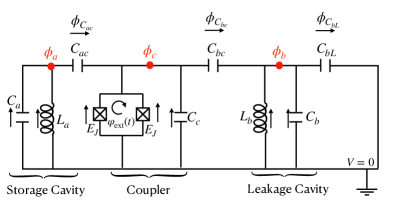
Figure 6: Quantum circuit of the emitter. The coupler is derived to properly transfer a quantum state from storage to the leakage cavity. Both cavities are shown by lumped elements which capacitively are coupled to a symmetry flux tunable transmon.

The quantum circuit of Fig. 2 is shown in detail in Fig. 6. We consider the two cavities as lumped elements including capacitances $C_{a(b)}$ in parallel with the inductances $L_{a(b)}$. The coupler is described by the total capacitance $C_{c}$, junction energy $E_{j}$, and the AC flux drive $\varphi_{\mathrm{ext}}(t)$. The coupler capacitively is coupled to the storage and leakage cavity through the capacitance $C_{ac},C_{bc}$, respectively. The capacitance $C_{bL}$ is the coupling between the leakage cavity and the transmission line which gives rise to a minor frequency shift of the leakage cavity. The red dots show the flux of each system with which the Lagrangian and the Hamiltonian of the system can be evaluated.

To properly drive the effective Hamiltonian we first evaluate the lagrangian of the quantum circuit $\mathcal{L}=\mathcal{T}-\mathcal{V}$ where $\mathcal{T}$ and $\mathcal{V}$ correspond to the kinetic and potential energy, respectively.

According to Fig. 6, the kinetic energy is evaluated as

$$\mathcal{T}=\frac{1}{2}\Bigg{[} C_{a}\dot{\phi}_{a}^{2}+C_{ac}\dot{\phi}_{C_{ac}}^{2}+C_{c}\dot{\phi}_{c}^{2}$$

$$+C_{bc}\dot{\phi}_{C_{bc}}^{2}+C_{b}\dot{\phi}_{b}^{2}+C_{bL}\dot{\phi}_{C_{bL}}^{2}\Bigg{]}$$ (18)

and the potential is

$$\mathcal{V}=\frac{1}{2}\Bigg{[}\frac{\phi_{a}^{2}}{L_{a}}+\frac{\phi_{b}^{2}}{L_{b}}\Bigg{]}-2E_{J}\cos(\frac{\pi\phi_{\mathrm{ext}}(t)}{\phi_{0}})\cos(\frac{2\pi\phi_{c}}{\phi_{0}}),$$ (19)

where the detail of the derivation of the coupler potential is provided in the appendix B. Using Kirchoff’s voltage laws

$$\dot{\phi}_{C_{ac}}=\dot{\phi}_{c}-\dot{\phi}_{a}\,,\,\,\,\,\dot{\phi}_{C_{bc}}=\dot{\phi}_{b}-\dot{\phi}_{c}\,,\,\,\,\,\dot{\phi}_{C_{bL}}=-\dot{\phi}_{b},$$ (20)

and the conjugate relation

$$Q_{i}=\frac{\partial\mathcal{L}}{\partial\dot{\phi_{i}}},i=a,c,b$$ (21)

the kinetic energy in the charge basis $[Q_{a},Q_{c},Q_{b}]$ is obtained as

$$\mathcal{T}=\frac{1}{2}\vec{Q}\mathcal{C}\vec{Q}^{T}$$ (22)

where

$$\mathcal{C}\approx\begin{bmatrix}\frac{1}{\mathbf{C_{a}}}&\,\,\,\,\frac{C_{ac}}{\mathbf{C_{a}}\mathbf{C_{c}}}&0\\ \\ \frac{C_{ac}}{\mathbf{C_{a}}\mathbf{C_{c}}}&\frac{1}{\mathbf{C_{c}}}&\frac{C_{bc}}{\mathbf{C_{b}}\mathbf{C_{c}}}\\ \\ 0&\frac{C_{bc}}{\mathbf{C_{b}}\mathbf{C_{c}}}&\frac{1}{\mathbf{C_{b}}}\end{bmatrix}.$$ (23)

In the capacity matrix, $\mathbf{C_{a}}=C_{a}+C_{ac},\mathbf{C_{c}}=C_{c}+C_{bc}+C_{ac},\mathbf{C_{b}}=C_{b}+C_{bc}+C_{bL}$. According to the capacitance matrix, the coupling strength between the coupler and the storage ( leakage ) cavity depends on $g_{ac}\propto\frac{C_{ac}}{\mathbf{C_{a}}\mathbf{C_{c}}},g_{bc}\propto\frac{C_{bc}}{\mathbf{C_{b}}\mathbf{C_{c}}}$, respectively, where we assume the coupling is weak $C_{ac},C_{bc}\ll C_{a},C_{b},C_{c}$.

A.1 Linear and nonlinear potential of the coupler

From Eq. (19), the potential energy of the coupler includes the contribution of the nonlinear flux operators and the external drive as

$$U_{\mathrm{coupler}}= -2E_{J}\cos(\frac{\pi\phi_{\mathrm{ext}}}{\phi_{0}})\cos(\frac{2\pi\phi_{c}}{\phi_{0}})$$

$$= -2E_{J}\cos(\frac{\varphi_{\mathrm{ext}}(t)}{2})\cos(\varphi_{c}),$$ (24)

where the reduced flux is considered as $\varphi_{c}=\frac{2\pi\phi_{c}}{\phi_{0}}$ and $\varphi_{\mathrm{ext}}(t)=\varphi_{\mathrm{dc}}+F(t)\sin(\omega_{d}t).$ Using the Taylor expansion

$$\cos(\varphi_{c})= 1-\frac{\varphi_{c}^{2}}{2}+\frac{\varphi_{c}^{4}}{4!}+\mathcal{O}(\varphi_{c}^{6}),$$ (25)

the potential energy of the transmon can be decomposed into a linear $U_{C}^{l}$ and nonlinear $U_{C}^{nl}$ terms as (the constant terms are dropped)

$$U_{\mathrm{coupler}}= \,U_{C}^{l}+U_{C}^{nl},$$

$$U_{C}^{l}= -2E_{J}\cos(\frac{\varphi_{\mathrm{ext}}(t)}{2})[1-\frac{\varphi_{c}^{2}}{2}],$$

$$U_{C}^{nl}= -2E_{J}\cos(\frac{\varphi_{\mathrm{ext}}(t)}{2})[\frac{\varphi_{c}^{4}}{4!}].$$ (26)

By expanding the flux drive term

$$\cos(\frac{\varphi_{\mathrm{ext}}(t)}{2})= \cos(\frac{\varphi_{\mathrm{dc}}}{2})-\frac{\sin(\frac{\varphi_{\mathrm{dc}}}{2})F(t)\sin(\omega_{d}t)}{2}$$

$$-\frac{\cos(\frac{\varphi_{\mathrm{dc}}}{2})}{8}F(t)^{2}\sin(\omega_{d}t)^{2}+\mathcal{O}(F(t)^{3}),$$ (27)

the quadratic part of the potential, second line of (A.1), can be decomposed into time-independent and time-dependent terms as

$$U_{C}^{l}=\, E_{J}\Bigg{[}\cos(\frac{\varphi_{\mathrm{dc}}}{2})\Bigg{]}\varphi_{c}^{2}$$

$$-E_{J}\Bigg{[}\frac{\sin(\frac{\varphi_{\mathrm{dc}}}{2})F(t)\sin(\omega_{d}t)}{2}$$

$$\,\,\,\,\,\,\,\,\,\,\,\,\,\,\,\,\,+\frac{\cos(\frac{\varphi_{\mathrm{dc}}}{2})}{8}F(t)^{2}\sin(\omega_{d}t)^{2}\Bigg{]}\varphi_{c}^{2}.$$ (28)

Consequently one can easily find the time-independent potential matrix $\mathcal{V^{\prime}}$ in basis $\phi=(\phi_{a},\phi_{c},\phi_{b})$

$$\mathcal{V^{\prime}}=\begin{bmatrix}\frac{1}{L_{A}}&0&0\\ \\ 0&\frac{8\pi^{2}E_{J}(\cos(\frac{\varphi_{\mathrm{dc}}}{2}))}{\phi_{0}^{2}}&0\\ \\ 0&0&\frac{1}{L_{B}}\end{bmatrix},$$ (29)

which makes the potential energy $\mathcal{V}=\frac{1}{2}\vec{\phi}\mathcal{V^{\prime}}\vec{\phi}^{T}$. Using the linear potential $\mathcal{V}$ and the Kinetic energy $\mathcal{T}$, the dressed mode of the circuit can be evaluated. In the dressed mode, the time-dependent and nonlinear terms of the potential of the coupler provide the value of the effective nonlinear interaction on the cavities and the optimal swap operator between the cavities, which are discussed in the next section.

A.2 Dressed modes and the effective Hamiltonian

To calculate the dressed mode of the circuit Fig. 6, one can define the linear and time-independent Hamiltonian as

$$H^{l}=\frac{1}{2}\vec{Q}\mathcal{C}\vec{Q}^{T}+\frac{1}{2}\vec{\phi}\mathcal{V^{\prime}}\vec{\phi}^{T}$$ (30)

where $\mathcal{C},\mathcal{V^{\prime}}$ are evaluated in Eqs. (23,29), respectively. The equation of motion for the Heisenberg operator is given by

$$\partial^{2}_{t}\vec{Q}^{T} =-\mathcal{V^{\prime}C}\vec{Q}^{T}$$

$$\partial^{2}_{t}\vec{\phi}^{T} =-\mathcal{CV^{\prime}}\vec{\phi}^{T},$$ (31)

and can be solved by making the ansatz

$$\vec{Q}^{T} =i\sum_{n}\sqrt{\frac{\hbar\omega_{n}}{2}}\frac{1}{\sqrt{\mathcal{C}}}\vec{\zeta}^{T}_{n}(a_{n}^{\dagger}e^{i\omega_{n}t}-a_{n}e^{-i\omega_{n}t})$$

$$\vec{\phi}^{T} =\sum_{n}\sqrt{\frac{\hbar}{2\omega_{n}}}\sqrt{\mathcal{C}}\vec{\zeta}^{T}_{n}(a_{n}^{\dagger}e^{i\omega_{n}t}+a_{n}e^{-i\omega_{n}t}).$$ (32)

The frequency of the modes $\omega_{n}$ and its corresponding orthogonal mode-functions $\vec{\zeta}_{n}$ follow from the eigenvalue equation

$$(\sqrt{\mathcal{C}}\mathcal{V^{\prime}}\sqrt{\mathcal{C}}-\omega_{n}^{2}\mathpzc{I})\vec{\zeta}^{T}_{n}=0,$$ (33)

where yields the uncoupled Hamiltonian

$$H^{l}/h=\sum_{n=1}^{3}\omega_{n}a_{n}^{\dagger}a_{n}.$$ (34)

The phase operator of the coupler $\phi_{c}$, in the new basis $a_{i}$, can be expressed as

$$\phi_{c}= \sum_{n=1}^{3}\frac{\lambda_{n}}{\sqrt{2}}(\hat{a}^{\dagger}_{n}+\hat{a}_{n})=\sum_{n=1}^{3}\frac{A_{n}+A^{\dagger}_{n}}{\sqrt{2}}$$

$$\longrightarrow\lambda_{n}=\sqrt{\frac{\hbar}{\omega_{n}}}\vec{e}_{c}\sqrt{\mathcal{C}}\vec{\zeta}_{n}^{T},$$ (35)

where indices $i=1,2,3$ correspond to $a,c,b$, respectively and we introduce new parameters representation

$$\lambda_{a} \equiv\lambda_{1}\,\,,\,\,\lambda_{c}\equiv\lambda_{2}\,\,,\,\,\lambda_{b}\equiv\lambda_{3}$$

$$a =a_{1},c=a_{2},b=a_{3},$$

$$\omega_{a} =\omega_{1},\omega_{c}=\omega_{2},\omega_{b}=\omega_{3}.$$ (36)

Considering a compact form of the flux of the tunable coupler nigg2012black ; marcos2013superconducting

$$\phi_{c}=\frac{1}{\sqrt{2}}(A_{a}+A_{a}^{\dagger}+A_{b}+A_{b}^{\dagger}+A_{c}+A_{c}^{\dagger})=\frac{A+A^{\dagger}}{\sqrt{2}}$$ (37)

and defining $\bar{\lambda}=[A,A^{\dagger}]=|\lambda_{a}|^{2}+|\lambda_{b}|^{2}+|\lambda_{c}|^{2}$, the time-dependent parts of Eq. (28) is obtained as

$$H^{l}(t)=\frac{-2E_{J}\pi^{2}}{\phi_{0}^{2}}\Bigg{[} \frac{\sin(\frac{\varphi_{\mathrm{dc}}}{2})F(t)\sin(\omega_{d}t)}{2}$$

$$+\frac{\cos(\frac{\varphi_{\mathrm{dc}}}{2})}{8}F(t)^{2}\sin(\omega_{d}t)^{2}\Bigg{]}(2A^{\dagger}A+\bar{\lambda}),$$ (38)

where provides the swap operator and the stark shifts. In addition, the fourth order of the flux operator, $U_{C}^{nl}$ in Eq. (A.1), provides selfKerr, crossKerr interaction, and also Stark shifts which in the dressed mode of Eq. (37) is obtained

$$U_{C}^{nl}=H_{nl}\approx \frac{-\pi^{4}E_{J}\cos(\frac{\varphi_{\mathrm{ext}}(t)}{2})}{3\phi_{0}^{4}}(A+A^{\dagger})^{4}$$

$$H_{nl}\approx \frac{-\pi^{4}E_{J}\cos(\frac{\varphi_{\mathrm{ext}}(t)}{2})}{3\phi_{0}^{4}}\Bigg{[}12\bar{\lambda}A^{\dagger}A+6A^{\dagger}A^{\dagger}AA\Bigg{]}.$$ (39)

If we consider the drive frequency $\omega_{d}=\omega_{b}-\omega_{a}$, the total Hamiltonian $H=$ 34+A.2+39, in the rotating frame $\omega_{a}a^{\dagger}a+\omega_{b}b^{\dagger}b+\omega_{c}c^{\dagger}c$ is obtained

$$H= -ig_{\mathrm{swap}}(t)[b^{\dagger}a-a^{\dagger}b]$$

$$+g_{Stark}(t)[\lambda_{a}^{2}a^{\dagger}a+\lambda_{b}^{2}b^{\dagger}b+\lambda_{c}^{2}c^{\dagger}c]$$

$$+g_{\mathrm{selfkerr}}[\lambda_{a}^{4}a^{2\dagger}a^{2}+\lambda_{b}^{4}b^{2\dagger}b^{2}+\lambda_{c}^{4}c^{2\dagger}c^{2}]$$

$$+g_{\mathrm{crosskerr}}[\lambda_{a}^{2}\lambda_{b}^{2}b^{\dagger}ba^{\dagger}a+\lambda_{a}^{2}\lambda_{c}^{2}c^{\dagger}ca^{\dagger}a+\lambda_{c}^{2}\lambda_{b}^{2}b^{\dagger}bc^{\dagger}c],$$ (40)

where the coefficients are evaluated as

$$g_{\mathrm{swap}}(t) =(\frac{\pi^{2}}{\phi_{0}^{2}}-\frac{\bar{\lambda}\pi^{4}}{\phi_{0}^{4}})E_{J}\lambda_{a}\lambda_{b}\sin(\frac{\varphi_{\mathrm{dc}}}{2})F(t),$$ (41)

$$g_{\mathrm{Stark}}(t) =(\frac{\bar{\lambda}\pi^{4}}{\phi_{0}^{4}}-\frac{\pi^{2}}{\phi_{0}^{2}})\frac{E_{J}\cos(\frac{\varphi_{\mathrm{dc}}}{2})}{4}F(t)^{2},$$ (42)

$$g_{\mathrm{selfkerr}} =\frac{-2\pi^{4}E_{J}\cos(\frac{\varphi_{\mathrm{dc}}}{2})}{\phi_{0}^{4}},$$ (43)

$$g_{\mathrm{crosskerr}} =\frac{-8\pi^{4}E_{J}\cos(\frac{\varphi_{\mathrm{dc}}}{2})}{\phi_{0}^{4}}.$$ (44)

It is worth noting that because the coupler is initialized in the ground state, the Hamiltonian (A.2), decouples the coupler from both cavities which means the terms $(c^{\dagger}ca^{\dagger}a,c^{\dagger}cb^{\dagger}b,c^{\dagger 2}c^{2})$ vanish at all times. Comparing Eqs. (III,A.2-44), the following parameters are introduced

$$\chi_{a(b)}= \frac{-2\pi^{4}E_{J}\cos(\frac{\varphi_{\mathrm{dc}}}{2})}{\phi_{0}^{4}}\lambda_{a(b)}^{4},$$

$$\chi_{ab}= \frac{-8\pi^{4}E_{J}\cos(\frac{\varphi_{\mathrm{dc}}}{2})}{\phi_{0}^{4}}\lambda_{a}^{2}\lambda_{b}^{2},$$

$$S_{a(b)}(t)= g_{\mathrm{Stark}}(t)\lambda_{a(b)}^{2}.$$ (45)

Appendix B Calculation of the potential of the coupler

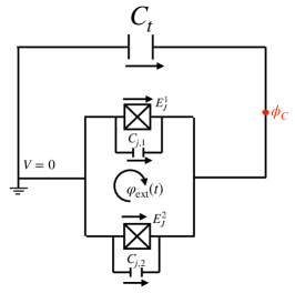
Figure 7: Schematic of a flux-tunable coupler. Two Josephson junction $E_{J}^{1},E_{J}^{1}$ are in parallel with two parasitic (small) capacitance $C_{j,1},C_{j,2}$ and shunted by a large capacitance $C_{t}$ rasmussen2021superconducting . The flux drive in the small loop is $\varphi_{\mathrm{ext}}(t)$ and the bigger loop is described by the flux operator $\phi_{C}$.

In general, we can consider each junction coupled in parallel with parasitic capacitance ($C_{j,1},C_{j,2}$), and the total system is shunted by a large capacitance $C_{t}$; see Fig. 8. The Kinetic and potential energy of this simple circuit is

$$\mathcal{T} =\frac{1}{2}\Bigg{[}C_{t}\dot{\phi}_{C}^{2}+C_{j,1}\dot{\phi}_{{j,1}}^{2}+C_{j,2}\dot{\phi}_{{j,2}}^{2}\Bigg{]}$$

$$\mathcal{V} =-E_{j,1}\cos(\frac{2\pi\phi_{j,1}}{\phi_{0}})-E_{j,2}\cos(\frac{2\pi\phi_{j,2}}{\phi_{0}})$$ (46)

According to the number of nodes in the circuit, it can be described by one degree of freedom which we consider $\phi_{C}$. Using the Kirchhoff voltage low, the small loop of junctions obeys the following equation

$$\phi_{j,1}-\phi_{j,2}=\phi_{\mathrm{ext}}.$$ (47)

In the following, we introduce the independent parameter $\phi_{C}$ as the function of the two fluxes across the junctions

$$m_{1}\phi_{j,1}+m_{2}\phi_{j,2}=\phi_{C}$$ (48)

Using Eq. (47,48) the fluxes are obtained as

$$\phi_{j,1} =\frac{\phi_{C}+m_{2}\phi_{\mathrm{ext}}}{m_{1}+m_{2}}$$

$$\phi_{j,2} =\frac{\phi_{C}-m_{1}\phi_{\mathrm{ext}}}{m_{1}+m_{2}},$$ (49)

where subsequently, the kinetic part of Eq. (B) can be rewritten as

$$\mathcal{T}=\frac{1}{2}\Bigg{[} [\frac{C_{j,1}+C_{j,2}}{(m_{1}+m_{2})^{2}}+C_{t}]\dot{\phi}_{C}^{2}$$

$$+\frac{2(m_{2}C_{j,1}-m_{1}C_{j,2})}{(m_{1}+m_{2})^{2}}\dot{\phi}_{C}\dot{\phi}_{\mathrm{ext}}+\mathcal{O}(\dot{\phi}_{\mathrm{ext}})^{2}\Bigg{]}.$$ (50)

We do not take the second order of the flux fluctuation into account, as we assume the flux drive is slow in time. To remove the effect of the flux drive fluctuation $\dot{\phi}_{\mathrm{ext}}$, one can utilize the following two conditions

$$m_{1}+m_{2} =1$$

$$m_{2}C_{j,1}-m_{1}C_{j,2} =0,$$ (51)

where leads to

$$m_{1} =\frac{C_{j,1}}{C_{j,1}+C_{j,2}}$$

$$m_{2} =\frac{C_{j,2}}{C_{j,1}+C_{j,2}}.$$

Hence $\mathcal{T},\mathcal{V}$ are obtained as

$$\mathcal{T} =\frac{C_{j,1}+C_{j,2}+C_{t}}{2}\dot{\phi}_{C}^{2}$$

$$\mathcal{V} =-E_{J,1}\cos(\frac{2\pi[\phi_{C}+m_{2}\phi_{\mathrm{ext}}]}{\phi_{0}})-E_{J,2}\cos(\frac{2\pi[\phi_{C}-m_{1}\phi_{\mathrm{ext}}]}{\phi_{0}}).$$ (52)

If we consider symmetry junction with $E_{J,1}=E_{J,2}=E_{J}$ and $C_{j,1}=C_{j,2}$, consequently $m_{1}=m_{2}=1/2$ and the potential energy can be simplified as

$$\mathcal{V}=-2E_{j}\cos(\frac{2\pi\phi_{C}}{\phi_{0}})\cos(\frac{\pi\phi_{\mathrm{ext}}}{\phi_{0}}),$$ (53)

which is equivalent to Eq. (19). Introducing $C_{c}\equiv C_{j,1}+C_{j,2}+C_{t}$, the same kinetic energy as in Equation (A) is obtained.

Appendix C Wigner Function of Fig. 4 (c)

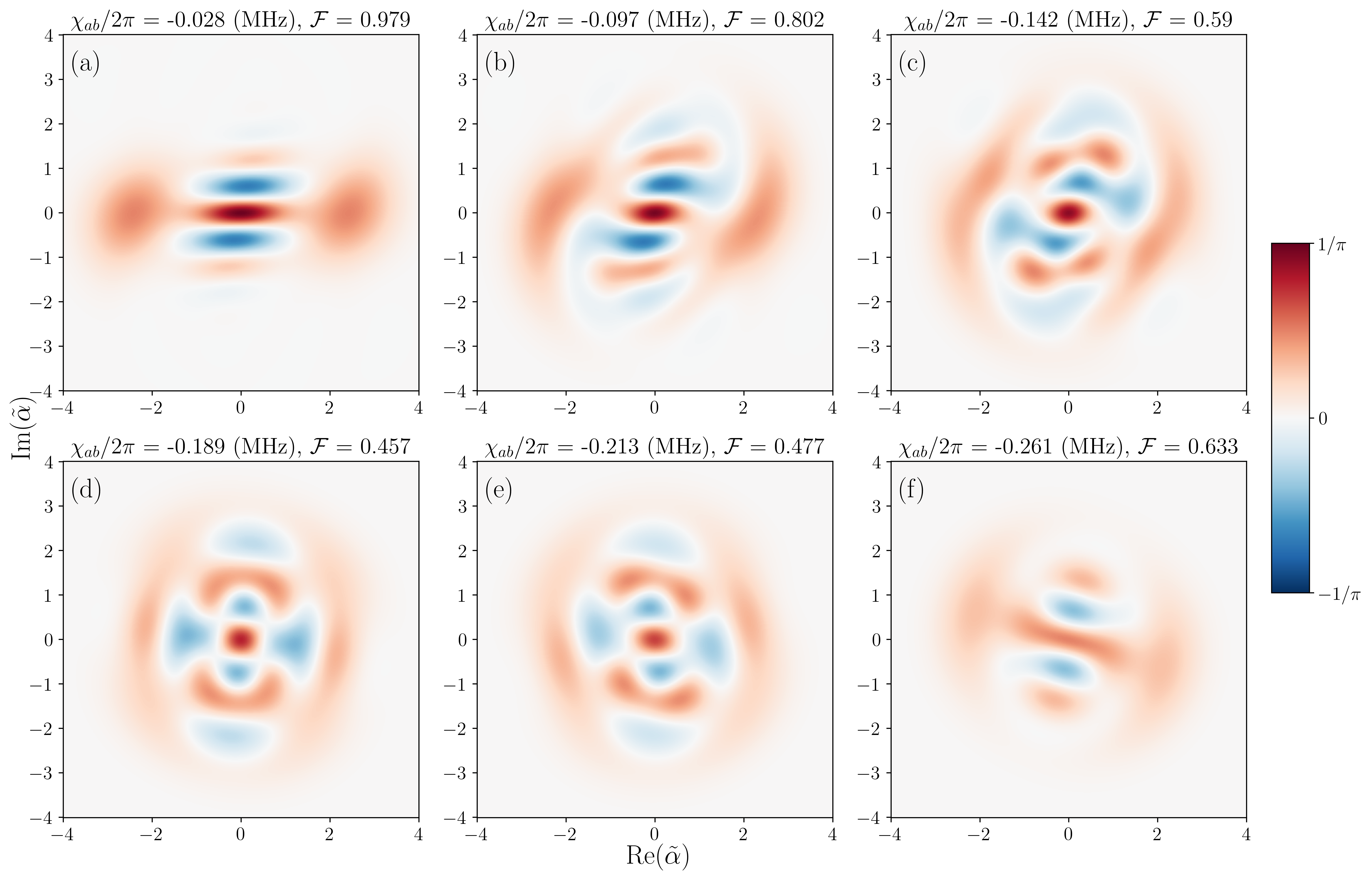
Figure 8: Different realizations of the Wigner functions of the single output mode TCCS in Fig. 4 (c).

References

• [1] H Jeff Kimble. The quantum internet. Nature, 453(7198):1023–1030, 2008.
• [2] Stephanie Wehner, David Elkouss, and Ronald Hanson. Quantum internet: A vision for the road ahead. Science, 362(6412):eaam9288, 2018.
• [3] Brian Vlastakis, Gerhard Kirchmair, Zaki Leghtas, Simon E Nigg, Luigi Frunzio, Steven M Girvin, Mazyar Mirrahimi, Michel H Devoret, and Robert J Schoelkopf. Deterministically encoding quantum information using 100-photon schrödinger cat states. Science, 342(6158):607–610, 2013.
• [4] Zaki Leghtas, Steven Touzard, Ioan M Pop, Angela Kou, Brian Vlastakis, Andrei Petrenko, Katrina M Sliwa, Anirudh Narla, Shyam Shankar, Michael J Hatridge, et al. Confining the state of light to a quantum manifold by engineered two-photon loss. Science, 347(6224):853–857, 2015.
• [5] Nissim Ofek, Andrei Petrenko, Reinier Heeres, Philip Reinhold, Zaki Leghtas, Brian Vlastakis, Yehan Liu, Luigi Frunzio, SM Girvin, Liang Jiang, et al. Extending the lifetime of a quantum bit with error correction in superconducting circuits. Nature, 536(7617):441–445, 2016.
• [6] Philippe Campagne-Ibarcq, Alec Eickbusch, Steven Touzard, Evan Zalys-Geller, Nicholas E Frattini, Volodymyr V Sivak, Philip Reinhold, Shruti Puri, Shyam Shankar, Robert J Schoelkopf, et al. Quantum error correction of a qubit encoded in grid states of an oscillator. Nature, 584(7821):368–372, 2020.
• [7] Shruti Puri, Lucas St-Jean, Jonathan A Gross, Alexander Grimm, Nicholas E Frattini, Pavithran S Iyer, Anirudh Krishna, Steven Touzard, Liang Jiang, Alexandre Blais, et al. Bias-preserving gates with stabilized cat qubits. Science advances, 6(34):eaay5901, 2020.
• [8] Zhongchu Ni, Sai Li, Xiaowei Deng, Yanyan Cai, Libo Zhang, Weiting Wang, Zhen-Biao Yang, Haifeng Yu, Fei Yan, Song Liu, et al. Beating the break-even point with a discrete-variable-encoded logical qubit. Nature, pages 1–5, 2023.
• [9] Arne L Grimsmo, Joshua Combes, and Ben Q Baragiola. Quantum computing with rotation-symmetric bosonic codes. Physical Review X, 10(1):011058, 2020.
• [10] Daiqin Su, Ish Dhand, and Timothy C. Ralph. Universal quantum computation with optical four-component cat qubits. Phys. Rev. A, 106:042614, Oct 2022.
• [11] Andrew Addison Houck, DI Schuster, JM Gambetta, JA Schreier, BR Johnson, JM Chow, L Frunzio, J Majer, MH Devoret, SM Girvin, et al. Generating single microwave photons in a circuit. Nature, 449(7160):328–331, 2007.
• [12] Mathieu Pierre, Ida-Maria Svensson, Sankar Raman Sathyamoorthy, Göran Johansson, and Per Delsing. Storage and on-demand release of microwaves using superconducting resonators with tunable coupling. Applied Physics Letters, 104(23):232604, 2014.
• [13] M. Pechal, L. Huthmacher, C. Eichler, S. Zeytinoğlu, A. A. Abdumalikov, S. Berger, A. Wallraff, and S. Filipp. Microwave-controlled generation of shaped single photons in circuit quantum electrodynamics. Phys. Rev. X, 4:041010, Oct 2014.
• [14] Sankar Raman Sathyamoorthy, Andreas Bengtsson, Steven Bens, Michaël Simoen, Per Delsing, and Göran Johansson. Simple, robust, and on-demand generation of single and correlated photons. Phys. Rev. A, 93:063823, Jun 2016.
• [15] P. Forn-Díaz, C. W. Warren, C. W. S. Chang, A. M. Vadiraj, and C. M. Wilson. On-demand microwave generator of shaped single photons. Phys. Rev. Appl., 8:054015, Nov 2017.
• [16] Wolfgang Pfaff, Christopher J Axline, Luke D Burkhart, Uri Vool, Philip Reinhold, Luigi Frunzio, Liang Jiang, Michel H Devoret, and Robert J Schoelkopf. Controlled release of multiphoton quantum states from a microwave cavity memory. Nature Physics, 13(9):882–887, 2017.
• [17] Christopher J Axline, Luke D Burkhart, Wolfgang Pfaff, Mengzhen Zhang, Kevin Chou, Philippe Campagne-Ibarcq, Philip Reinhold, Luigi Frunzio, SM Girvin, Liang Jiang, et al. On-demand quantum state transfer and entanglement between remote microwave cavity memories. Nature Physics, 14(7):705–710, 2018.
• [18] Daniele Cozzolino, Beatrice Da Lio, Davide Bacco, and Leif Katsuo Oxenløwe. High-dimensional quantum communication: benefits, progress, and future challenges. Advanced Quantum Technologies, 2(12):1900038, 2019.
• [19] Luke D Burkhart, James D Teoh, Yaxing Zhang, Christopher J Axline, Luigi Frunzio, MH Devoret, Liang Jiang, SM Girvin, and RJ Schoelkopf. Error-detected state transfer and entanglement in a superconducting quantum network. PRX Quantum, 2(3):030321, 2021.
• [20] Jiaying Yang, Axel Eriksson, Mohammed Ali Aamir, Ingrid Strandberg, Claudia Castillo Moreno, Daniel Perez Lozano, Per Persson, and Simone Gasparinetti. Deterministic generation of shaped single microwave photons using a parametrically driven coupler. arXiv preprint arXiv:2303.02899, 2023.
• [21] Philip Krantz, Morten Kjaergaard, Fei Yan, Terry P Orlando, Simon Gustavsson, and William D Oliver. A quantum engineer’s guide to superconducting qubits. Applied physics reviews, 6(2):021318, 2019.
• [22] Alexandre Blais, Arne L Grimsmo, Steven M Girvin, and Andreas Wallraff. Circuit quantum electrodynamics. Reviews of Modern Physics, 93(2):025005, 2021.
• [23] Yi Yin, Yu Chen, Daniel Sank, PJJ O’Malley, TC White, R Barends, J Kelly, Erik Lucero, Matteo Mariantoni, A Megrant, et al. Catch and release of microwave photon states. Physical review letters, 110(10):107001, 2013.
• [24] Marek Pechal, Lukas Huthmacher, Christopher Eichler, Sina Zeytinoğlu, AA Abdumalikov Jr, Simon Berger, Andreas Wallraff, and Stefan Filipp. Microwave-controlled generation of shaped single photons in circuit quantum electrodynamics. Physical Review X, 4(4):041010, 2014.
• [25] Alexander Holm Kiilerich and Klaus Mølmer. Input-output theory with quantum pulses. Physical review letters, 123(12):123604, 2019.
• [26] Heinz-Peter Breuer, Francesco Petruccione, et al. The theory of open quantum systems. Oxford University Press on Demand, 2002.
• [27] Crispin Gardiner and Peter Zoller. Quantum noise: a handbook of Markovian and non-Markovian quantum stochastic methods with applications to quantum optics. Springer Science & Business Media, 2004.
• [28] Michael Tinkham. Introduction to superconductivity. Courier Corporation, 2004.
• [29] Jens Koch, Terri M. Yu, Jay Gambetta, A. A. Houck, D. I. Schuster, J. Majer, Alexandre Blais, M. H. Devoret, S. M. Girvin, and R. J. Schoelkopf. Charge-insensitive qubit design derived from the cooper pair box. Phys. Rev. A, 76:042319, Oct 2007.
• [30] SE Rasmussen, KS Christensen, SP Pedersen, LB Kristensen, T Bækkegaard, NJS Loft, and NT Zinner. Superconducting circuit companion—an introduction with worked examples. PRX Quantum, 2(4):040204, 2021.
• [31] Simon E Nigg, Hanhee Paik, Brian Vlastakis, Gerhard Kirchmair, Shyam Shankar, Luigi Frunzio, MH Devoret, RJ Schoelkopf, and SM Girvin. Black-box superconducting circuit quantization. Physical Review Letters, 108(24):240502, 2012.
• [32] David Marcos, Peter Rabl, Enrique Rico, and Peter Zoller. Superconducting circuits for quantum simulation of dynamical gauge fields. Physical review letters, 111(11):110504, 2013.
• [33] P. T. Cochrane, G. J. Milburn, and W. J. Munro. Macroscopically distinct quantum-superposition states as a bosonic code for amplitude damping. Phys. Rev. A, 59:2631–2634, Apr 1999.
• [34] A. P. Lund, T. C. Ralph, and H. L. Haselgrove. Fault-tolerant linear optical quantum computing with small-amplitude coherent states. Phys. Rev. Lett., 100:030503, Jan 2008.
• [35] Zaki Leghtas, Gerhard Kirchmair, Brian Vlastakis, Robert J. Schoelkopf, Michel H. Devoret, and Mazyar Mirrahimi. Hardware-efficient autonomous quantum memory protection. Phys. Rev. Lett., 111:120501, Sep 2013.
• [36] Mazyar Mirrahimi, Zaki Leghtas, Victor V Albert, Steven Touzard, Robert J Schoelkopf, Liang Jiang, and Michel H Devoret. Dynamically protected cat-qubits: a new paradigm for universal quantum computation. New Journal of Physics, 16(4):045014, 2014.
• [37] Howard J Carmichael. Quantum trajectory theory for cascaded open systems. Physical review letters, 70(15):2273, 1993.
• [38] CW Gardiner. Driving a quantum system with the output field from another driven quantum system. Physical review letters, 70(15):2269, 1993.
• [39] NE Frattini, U Vool, S Shankar, A Narla, KM Sliwa, and MH Devoret. 3-wave mixing josephson dipole element. Applied Physics Letters, 110(22):222603, 2017.
• [40] Benjamin J Chapman, Stijn J de Graaf, Sophia H Xue, Yaxing Zhang, James Teoh, Jacob C Curtis, Takahiro Tsunoda, Alec Eickbusch, Alexander P Read, Akshay Koottandavida, et al. A high on-off ratio beamsplitter interaction for gates on bosonically encoded qubits. arXiv preprint arXiv:2212.11929, 2022.
• [41] Juan Ignacio Cirac, Peter Zoller, H Jeff Kimble, and Hideo Mabuchi. Quantum state transfer and entanglement distribution among distant nodes in a quantum network. Physical Review Letters, 78(16):3221, 1997.