Testing of on-cloud Gaussian Boson Sampler “Borealis” via graph theory

Abstract

Quantum photonic processors are emerging as promising platforms to prove preliminary evidence of quantum computational advantage towards the realization of universal quantum computers. In the context of non-universal noisy intermediate quantum devices, photonic-based sampling machines solving the Gaussian Boson Sampling problem currently play a central role in the experimental demonstration of a quantum computational advantage. In particular, the recently developed photonic machine Borealis, a large-scale instance of a programmable Gaussian Boson Sampling device encoded in the temporal modes of single photons, is available online for external users. In this work, we test the performances of Borealis as a sampling machine and its possible use cases in graph theory. We focused on the validation problem of the sampling process in the presence of experimental noise, such as photon losses, that could undermine the hardness of simulating the experiment. To this end, we used a recent protocol that exploits the connection between Guassian Boson Sampling and graphs perfect match counting. Such an approach to validation also provides connections with the open question on the effective advantage in using noisy Gaussian Boson Sampling devices for graphs similarity and isomorphism problems.

I Introduction

Quantum devices and quantum algorithms promise substantial advantages in many computational tasks. Such applications include as notable examples quantum computing, simulation, communication, and sensing. In recent years, an ever-increasing number of advancements is being made in this field, with the first experiments [1, 2, 3, 4, 5, 6] tackling the quantum advantage regime, namely the scenario where quantum devices are capable of outperforming classical computers in specific tasks. These results have thus opened the way for the development and application of noisy intermediate-scale quantum (NISQ) processors [7] for quantum-enhanced information processing.

An example of a non-universal quantum processor is the Gaussian Boson Sampling (GBS) scheme. It is a variant of the original proposal of Boson Sampling (BS), which is a classically-hard computational problem that can be tackled through the use of dedicated quantum photonic devices. More precisely, GBS is the problem of generating samples from the photon-counting output distribution of indistinguishable Gaussian states of light after the evolution through a multi-mode random linear optical interferometer [8, 9, 10, 11, 12]. This problem is intractable for a classical computer when the input states are indistinguishable sources of single-mode squeezed states. Then, a dedicated quantum photonic device can tackle such a task more efficiently, thus corresponding to a quantum computational advantage for a problem instance of sufficient size. The GBS problem has thus drawn attention in the photonic community due to the practical chance to achieve the quantum advantage regime with the technology available today. The latest GBS instances have reached the condition where the quantum device has solved the task faster than current state-of-the-art classical strategies in several experiments [2, 4, 6], including the Borealis machine by the company Xanadu [5]. Further interest in the GBS scheme is motivated by the connection between the sampling process and the problem of counting perfect matchings of arbitrary graphs. In fact, an important property of GBS is that it is possible to encode an adjacency matrix of a graph in the device by proper tuning of the interferometer parameters and the squeezing values. Thus, the collected samples could be used to learn several properties of the graph, and be employed to solve some relevant problems in the field such as finding the dense subgraphs and max-clique, simulating vibronic spectra, and graph similarity [13]. Recently, GBS-based algorithms to solve such well-known problems in graph theory have been formulated [14, 15, 16]. First tests on quantum devices have been then performed on small-scale integrated photonics devices [17] and on larger dimensions in bulk optics through time- [18, 19] and path-encoded interferometers [20].

In recent years large efforts have been devoted to developing more efficient classical algorithms capable of simulating the sampling process [21, 22, 23, 24, 25, 26, 27, 28, 29, 30], with the motivation of investigating the classical simulatability threshold of GBS devices. In this context, further studies had individuated sources of experimental noise that could undermine the hardness of the problem and allow for classical simulations [31], such as photon losses [32, 33, 34, 35, 36, 37] and photon distinguishability [38, 39, 40, 41]. Thus, the benchmarking of a GBS experiment can be performed by following a validation approach, i.e. a test that discerns when samples are drawn from classical simulatable models. The methods vary from Bayesian tests [42, 3, 43], statistical properties of two-point correlation functions [44, 45, 46] or long order ones [3], properties of marginal probabilities [40, 47, 48], to a very recent method based on the feature vectors components of the graph encoded in the device [49].

In this work, we focus on testing the performance of the Gaussian Boson Sampler Borealis [5], which recently claimed quantum advantages and has been made available on the cloud on Xanadu Cloud [50] and on Amazon Braket [51]. Some properties of the device have been recently investigated in Ref. [52] by remote users. The authors measured the quadrature coherence scale to find genuine signatures of the features of single-mode bosonic systems in the phase space representation. Here, we applied a validation approach to assess the device operation. In particular, we used the method based on graphs feature vectors [49] to exclude that Borealis samples collected in a real experiment subjected to noise can be compatible with some relevant classically-simulatable modes, that is, thermal, coherent, squashed or distinguishable particles samplers. First, in Section II we will provide background information on Gaussian Boson Sampling. Then, in Section III we will review the main features of the structure of Borealis. After that, in Section IV we will explain the process for interfacing with Borealis, while finally in Section V we will analyze the collected data and perform the validation of Borealis against the aforementioned alternative models.

II Background on Gaussian Boson Sampling

GBS is a linear-optics scheme to generate samples drawn from the photon-counting distribution generated by Gaussian light sources at the outputs of a multi-mode interferometer [10, 11, 12]. Such a sampling task is hard to simulate for certain classes of Gaussian states such as indistinguishable sources of single-mode squeezed vacuum (SMSV) states. The hardness is preserved in noisy experimental conditions as long as the levels of losses and photon distinguishability are limited.

Consider $m$ independent sources of Gaussian states $\rho_{i}$ without displacement such that the input is $\rho=\bigotimes_{i=1}^{m}\rho_{i}$ with a $2m\times 2m$ covariance matrix $\sigma$. The probability distribution of detecting $n$ photons in the configuration $\vec{n}=(n_{1},n_{2},...,n_{m})$, where $n_{i}$ is the number of photon in the output $i$ and $\sum_{i=1}^{m}n_{i}=n$, is

$$P(\vec{n})=|\sigma_{Q}|^{-1/2}\frac{\text{Haf}(A_{\vec{n}})}{\prod_{i=1}^{m}n_{i}!}$$ (1)

The quantity $\sigma_{Q}$ corresponds to $\sigma+I_{2m}$, being $I_{2m}$ the $2m\times 2m$ identity matrix, and Haf to the hafnian operation of the $2n\times 2n$ sub-matrix $A_{\vec{n}}$. Such a sub-matrix ($A_{\vec{n}}$) is individuated by taking $n_{i}$ times the $i$th row and the $i+m$-th column of $A$, and the hafnian is the operation that counts the number of perfect-matching in a graph represented by a symmetric adjacency matrix. The whole $2m\times 2m$ matrix $A$ has the following structure

$$A=\left(\begin{array}[]{cc}B&C\\ C^{T}&B^{*}\end{array}\right)$$ (2)

where $B$ is an $m\times m$ symmetric matrix and $C$ an $m\times m$ hermitian one. Both blocks depend on the transformation $U$ implemented by the interferometer and on the input Gaussian state. For example, the matrix representing $m$ indistinguishable SMSV states with squeezing parameters $s_{i}$ in a lossless experiment has $C=0$ and $B=U\text{diag}(\tanh{s_{1}},\dots,\tanh{s_{m}})U^{T}$. In this case, the adjacency matrix of a graph can be encoded in $B$ by tuning $U$ and $s_{i}$ values. For this reason, GBS with SMSV states had attracted lots of attention not only for proving a quantum advantage in the sampling task but also for applications on graphs, such as the problems of finding densest sub-graphs, the max-clique [14, 18] and graphs similarity [15, 16, 17]. The opposite scenario is a thermal sampler in which there is no coherence among the possible number of emitted photons that result in $A$ matrix with $C\neq 0$ only.

Many approaches have been proposed to validate GBS experiments in the quantum advantage regime [42, 44, 45, 46, 49]. The goal of a validation algorithm is to exclude that the samples are drawn from classical simulatable distributions such as the outputs of thermal, coherent, squashed and distinguishable Gaussian samplers. In this work, we apply a recent method introduced in Ref. [49] that makes use of graphs feature vectors estimated from GBS samples. The components of such vectors are called orbits, which result from a coarse-graining of the output configurations. More precisely, the method consists in the classification of different samplers in the space spanned by the three feature vector components identified by the probability of the orbits $O_{1}=[1,1,1,1,...]$, $O_{2}=[2,1,1,1,...]$ and $O_{3}=[2,2,1,1,...]$ for a given number $n$ of detected photons. The three orbits collect respectively the output states in which the number of photons in the modes is 0 or 1, in which only one detector measures two photons, and in which two modes host two photons. Plotting the feature vectors in the space $\{O_{1},O_{2},O_{3}\}$ allows us to distinguish between various types of classical samplers.

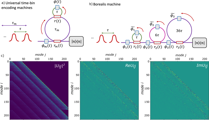
Figure 1: Time-bin encoding machines and Borealis structure. a) Example of universal time-bin interferometers. In such an encoding the optical modes are discrete time bins. The unitary operation over the modes is performed by two concatenated fiber loops. The shortest loop covers the time separation between two consecutive time bins, while the longest one covers the whole time duration of the number of modes. The same squeezing source is excited at each pulse, and photon counting measurements are performed at the end of the evolution. b) Structure of Borealis [53, 5]. The interferometer comprises three consecutive loops of increasing length. c) Example of a unitary matrix $U_{ij}$ performed by Borealis that shows the limited connectivity among the modes due to the loops structure.

III Structure of Borealis as a time-bin GBS

Borealis is based on time-domain multiplexing (TDM) [54, 5]. A single squeezed-light source emits batches of $m$ time-ordered squeezed-light pulses that interfere with one another with the help of optical delay loops, programmable beamsplitters (BSgate), and phase shifters (Rgate). The loops arrangement reported in Fig. 1a is an example of a universal time-bin interferometer able to encode any operation over the modes (see also Refs. [55, 56]). The transformation is controlled by time modulations of the splitting ratios of two BSgates [$r_{m}(t)$ and $r(t)$] and of the two phases of the Rgates [$\phi_{m}(t)$ and $\phi(t)$]. The two loops are concatenated and cover the time separation $\tau$ between consecutive bins and the whole time duration of the $m$ modes, $\tau_{m}=m\tau$, respectively. This architecture has been recently employed to realize a programmable and universal interferometer encoded in the time-bin for GBS applications [19].

The loops structure of Borealis does not follow the universal layout. Fig. 1b shows the time-bin interferometer that comprises 3 consecutive loops with 3 tunable BSgates $r_{1,2,3}(t)$ and likewise tunable Rgates $\phi_{1,2,3}(t)$. The tunable phase-shifters are limited to the range $[-\frac{\pi}{2},\frac{\pi}{2}]$. There are further 3 static phases $\tilde{\phi}_{1,2,3}$ that cannot be controlled by the user and represent the optical phases of each loop. The time separation between the bins is $\tau=167$ ns. Then, the time that covers the evolution of the 216 logical modes plus the 43 ancillary modes of the device is 43.5 $\mu$s and thus coincides with the time needed to obtain one sample from the device. The length of the 3 loops covers a time delay equal to $\tau$, $6\tau$ and $36\tau$ respectively. The squeezer has 4 settings for the squeezing parameter, “low”, “medium”, “high” and 0. The squeezing must be set to one of the allowed values and it cannot be modulated over the temporal modes. The setup ends with the single photons detection stage. The time bins are translated into 16 different spatial modes by a time-to-space demultiplexer system. Single photons are then detected by 16 photon-number-resolving detectors [5].

The design of Borealis has been chosen to be a compromise between the need for a programmable device and the requirement to achieve the quantum advantage regime. The architecture presents enough connectivity to have randomness in the transformation and to cover high-dimensional spaces with minimized losses and optical resources [12]. For connectivity, we mean the number of modes with which each of the modes interacts directly. In Borealis, for example, the loop structure allows each mode to be connected with at most 6 time bins. Thus, the 3-loop connectivity of Borealis puts some restrictions on the matrices that can be represented, as we can see in Fig. 1c. The transfer matrix is limited to being 0 on the upper half of the diagonal. The moduli of the matrix elements decrease when descending from the diagonal. They increase only every 6 and 36 modes, but are still smaller than the values at 6 or 36 modes above. Other restrictions derive from the ranges of tunability of the Rgates that do not allow the encoding of meaningful graphs adjacency matrices inside the device.

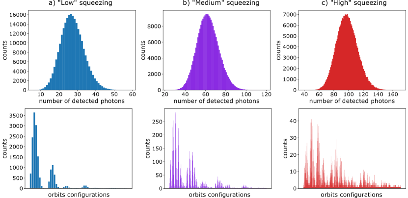
Figure 2: Detected photons and orbits probability distributions. On the top row, the distributions of the number of detected photons for the three levels of squeezing, a) “low”, b) “medium”, c) “high”. On the bottom, the distributions of the orbit configurations for the number of detected photons associated to the highest probability, namely $n=$26 for “low” squeezing, $n=$62 for “medium”, and $n=$97 for “high” squeezing. The x-axis represents the various orbits configuration ordered as follows, first $[1,1,1,\dots]$, then $[2,1,1,\dots]$, $[2,2,1,\dots]$, etc. The y-axis represents the number of samples for that orbit configuration. The size of each sample was 250000 shots.

IV Interfacing with Borealis

Borealis was accessed through Amazon Braket [51], and the parameters sent were the squeezing values, the parameters of the 3 beamsplitters and the parameters of the 3 phase shifters for each time mode, as well as the number of shots (i.e. the number of samples). The parameters sent are for 259 time modes, even though the number of outputs that we show is 216. This is because the first 43 modes are used to fill the loops, and thus the output for those first 43 modes is basically background noise. The device thus has 216 “logical” modes, while it has 259 “physical” modes.

When interfacing with Borealis one also downloads the device certificate, which describes the current calibration of the device. It contains information such as the loop phases, the squeezing values for the various settings, and the various efficiencies. The certificate distinguishes between 3 types of efficiencies:

• common efficiency, which corresponds to the balanced losses of the device independent from the implemented circuit.

• loop efficiencies, which correspond to the losses of each loop (3 values, one for each loop).

• relative channel efficiencies, which correspond to the relative efficiencies of the detectors (16 values, one for each detector).

The amount of the losses changed on a daily basis. The average number of photons in the output from Borealis was usually around $\sim$75% less than that of a lossless simulation with the same parameters.

The information included in the device certificate is necessary to perform numerical simulations with alternative models such as thermal samplers, which are used for comparison to assess the operation of Borealis. One aspect to be taken into account regarding the device certificate is that it is measured once a day, right before the 2-hour period in which Borealis is available. Thus, it could be less representative of the state of Borealis in those runs far away from the calibration. Indeed, the values of these efficiencies seem to oscillate over time, as we will show in Section V. After some discussion with Xanadu’s team, it turned out that these oscillations in the common efficiency are mainly due to variations in temperature. The scale of these variations in efficiency varies on a daily basis, with some days being more stable than others.

Another aspect to be taken into account regarding the device certificate is that simulations based on the included parameters, in particular with respect to noise, do not always accurately reproduce some features of the machine output. For instance, in some cases we found that the difference in the average number of detected photons per shot between the simulations performed according to the certificate parameters and the measured samples was small. This indicated that the loss estimation in the device certificate was accurate. In other cases, the mismatch between simulation and experiment was significantly higher, around 1.5-2 photon difference on an average number of photons of $\sim 26$, a value not compatible with statistical fluctuations. In these trials, the device certificate did not represent the physical device with sufficient accuracy within the statistical errors of the apparatus. This issue started to be more evident after one maintenance period that was made near the end of January 2023. Such discrepancy is relevant when trying to compare the experimental samples with simulations of classical samplers in the validation stage of the device, as it is no longer possible to have a truly accurate simulation for those days.

V Borealis data acquisition and validation

We will now analyze the results of our runs on Borealis, and compare them with some simulations. All of the code to interface with Borealis, perform the simulations, and analyze the data was written in Python 3 [57], and was based mainly on the libraries Strawberry Fields [58] and The Walrus [59].

In Fig. 2 we report the distribution of the number of detected photons at the Borealis outputs for the three squeezing levels larger than zero. Our goal is to apply the orbits method to validate our data against classically simulatable models such as thermal, coherent, squashed and distinguishable SMSV input states. The method of comparing the orbits is effective even in the quantum advantage regime as long as the number of modes $m$ is considerably larger than the number of detected photons [49]. The reason is that in such a condition the probability distribution of the various orbits configuration is peaked on a few orbits. This is evident in Fig. 2 in which the experimental orbits distributions for the three squeezing levels are reported. For this reason, all the runs shown in this section were made with the squeezing parameter set to “low”, which satisfies the condition $m\gg n$.

To check the stability of the results over time, we ran sampling experiments with the same settings of the circuit for two weeks. We executed two runs of 250000 shots each day from Monday to Friday for these two weeks. The parameters we used are the following: all beamsplitters are set to a transmissivity of $50\%$, and all phase shifters are set to $0$. We notice that the observed changes in the average number of detected photons in the outputs during the days impacts significantly the probability of orbits $\{O_{1},O_{2},O_{3}\}$. This variation is likely mostly due to changes in the common efficiency between days, as mentioned in the previous section. The plot of the three orbits probability for the 2 weeks is shown in Fig. 3, while in Table 1 we report the average number of photons per each run of the day during the two weeks.

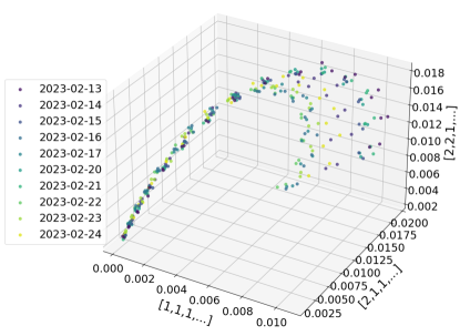
Figure 3: Stability check of Borealis total efficiency over days. Orbits distribution for the 2 weeks of runs with the same circuit settings. The variations in the different days are due to changes in the total efficiency of the apparatus, which is mostly dominated by the variations in common efficiency. The points correspond to the three orbits’ probability for detected photons in the range between 18 and 32 photons. More precisely, each point on the plot is associated with a specific detected photon number. The points at the bottom left corner correspond to 32 photons, while the points on the right are the orbits for 18 post-selected photons.

Day	13/02	14/02	15/02	16/02	17/02
Run 1	23.86	24.98	24.20	25.77	26.03
Run 2	23.61	24.64	24.21	26.01	25.81
Day	20/02	21/02	22/02	23/02	24/02
Run 1	24.15	23.85	25.98	25.45	25.21
Run 2	24.16	23.99	26.05	25.43	24.70

Table 1: Variation in the number of detected photons over days. Average number of photons in each run of the 2 weeks acquisitions performed by setting the same matrix. The relative standard deviation caused by the limited number of shots (250000) is $\sim$ 0.04% , which leads to a standard deviation in the mean photon number of around 0.01 photons. We thus observe that the mean number of photons in Borealis varies on each run performed in different days, and in some days this can even vary from a run to the next one, resulting in the orbits for the two runs of that day being further apart than the expectations.

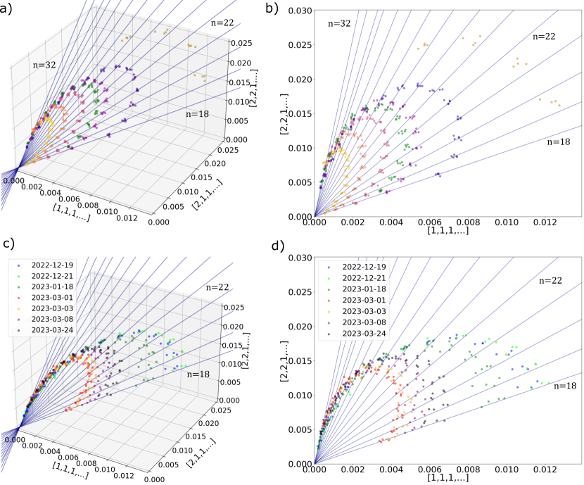
Figure 4: Role of losses in the orbits estimation. a-b) Orbits for the thermal sampler simulations. All points, except the green and dark gold ones, represent orbits where only the common efficiency has been changed. The lower the efficiency, the larger the radius of the orbits. The green points represent the case where one of the detectors was turned off, thus producing an unbalanced loss. The dark gold points are from the lossless indistinguishable SMSV states simulation. The details on the parameters used for the simulations can be found in Appendix A The lines are obtained by making a linear fit on all points with the same number of detected photons, excluding the points of the orbit with unbalanced losses and the SMSV simulation. Each line represents a different number of photons. We highlighted the number of corresponding photons for some of the lines in the figure. The effect of balanced losses is to move points along the lines. The unbalanced ones move the points away from the lines, but keep them on the same hyperplane. However, such an effect is evident only in the case of a strong amount of unbalancement. The lossless SMSV states points are not on those lines, but still on the same hyperplane. We report the projection of the orbits in the plane in b). c-d) Experimental orbits from the runs on Borealis. The lines are the same as the panel above calculated from the simulation with thermal states.

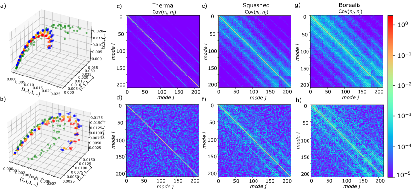
Figure 5: Validation of Borealis samples. a-b) Comparison of the orbits of Borealis (red), thermal states simulation (blue), squashed states simulation (orange) and coherent states simulation (green). The coherent, squashed, and thermal states simulations used the same parameters and device certificate of the Borealis runs. All the points were calculated on a sample size of 250000 shots with squeezing set to “low”. a) Borealis data collected in different days with different $U$ transformations. Such runs display a similar average number of detected photons and device certificates. b) Borealis data collected on the same day with different unitary transformations. In that day, the fluctuation in the average number of detected photons between runs on Borealis was compatible with statistical fluctuations, and the deviations of the average number of detected photons predicted by the simulations according to the certificate with those measured on the device were small. c-h) Comparison of the covariances of lossy thermal states, lossy squashed states, and Borealis for a given transformation $U$ of the device. The same circuit parameters were used for the simulations and the measurements with Borealis. The same device certificate was used for all the simulations. c) Covariance of the simulated thermal sampler with losses. d) Covariance of the thermal sampler with losses calculated from 250000 samples, to reproduce the additional noise due to a limited number of samples. e) Simulated covariance of a squashed light sampler with the losses of the Borealis circuit. f) Covariance of squashed light sampler from a finite sample of 250000 shots. g) Simulated covariance of an SMSV GBS with losses. h) Covariance of Borealis samples.

We now discuss the validation of the samples collected from Borealis. Based on the results reported in Ref.[49], we expect that indistinguishable SMSV GBS and indistinguishable thermal samples display orbits on the same hyperplane in the space spanned by $\{O_{1},O_{2},O_{3}\}$. Furthermore, in the lossless case thermal and squeezed light GBS have a similar spread of points in the orbits, while coherent has a spread of points that is much larger. The presence of photon distinguishability results in a change of such a hyperplane for both squeezed, thermal and coherent light. The effect of the photon losses is to change the GBS orbits towards the thermal sampler [49]. In fact, both balanced (the common efficiency in Borealis) and unbalanced (loop and relative detector efficiencies) losses lead to changes in the orbits but always on the same hyperplane. In Fig. 4a and b, we show in more detail such behaviors. The simulation considers thermal light inputs evolving through the transformation performed by the Borealis circuit with different levels of common efficiencies. We set the parameters of the circuit as follows: the transmittance of BSgates was set randomly between 0.4 and 0.6, while the phase shifters were set to random values in their full range $[-\frac{\pi}{2},\frac{\pi}{2}]$. The points that correspond to the same number of detected photons move along lines. More precisely, the orbits somehow expand when the common efficiency decreases, and shrink when the efficiency increases. Unbalanced losses, on the other hand, tend to alter the orbits, moving the points away from those lines, but still keeping the orbit on that same hyperplane. We also made an approximate simulation of the orbits of an ideal GBS, as can be seen in Fig. 4a-b. From this simulation we observe that those orbits reside on the same hyperplane of the thermal ones, as expected. However, they do not align with the lines of the thermal sampler.

In Fig. 4c-d, we compare runs taken in around 3 months, from the end of December 2022 to March 2023, with a break in January for maintenance. The circuit settings were the same that we employed for the numerical simulations with thermal light. The changes in the orbits are compatible with changes in the common efficiency observed during the time of data collection. The other interesting behavior is that the orbits seem to follow closely the lines from the thermal simulations. However, they do to not match exactly those lines. Thus, according to this tests Borealis appears to behave as a lossy GBS with squeezed states, which suggests that the orbits may be intermediate between a GBS with indistinguishable thermal light and a lossless squeezed light GBS. Furthermore, the orbits still lay on the same hyperplane of the thermal, as for the case of a lossy GBS with indistinguishable emitters. This allows us to exclude that the samples derive from a distinguishable particle sampler. Since we have shown that changes in losses do not change the hyperplane of the thermal simulation, from our analysis we can restrict the hypothesis to a scenario where Borealis is either a thermal with losses, a coherent with losses, a squashed with losses, or an SMSV GBS with losses. We will now proceed to show that it is not a coherent light sampler, and then we will show that it is closer to an SMSV GBS than a thermal or a squashed one.

In Fig. 5a we compare data from runs of 250000 samples from Borealis on different days but with the same average number of detected photons (red points), with simulated samples from coherent (green), squashed (orange) and thermal light (red). In panel b we consider runs performed on the same day in which the device certificate was providing an accurate estimate of the noise in the experiment due to photon losses. The orbits of coherent light are distant from Borealis data in both cases, and have a significantly bigger spread than the orbits of Borealis and of the thermal simulations. As a side note, we can also see that the orbits of the coherent sampler are distinct from those of a thermal sampler. In fact, even the mean photon number is different between the simulations of coherent and thermal samplers, indicating that losses affect the two class of states differently, given their different photon statistic. On the other hand, both Borealis and the thermal sampler seem to be affected in a very similar way by the losses, at least in terms of the mean photon number. Now, we are left only with the task of showing whether Borealis is closer to a thermal sampler, a squashed sampler, or an SMSV GBS with losses.

Squashed states are the closest classical model to the lossy SMSV sampler. Samples drawn from the probability distribution of squashed states are obtained using classical mixtures of coherent states [43, 60], similarly to the thermal sampler [61]. As we can see in Fig. 5a-b, the orbits of Borealis and of the thermal and squashed simulations are similar. This means that in this case, the orbits alone are not enough to ascertain whether Borealis is more likely to be a GBS with SMSV input states, a squashed sampler, or a thermal sampler. To further distinguish between these three cases, we look also at their respective sample covariance $\mathrm{Cov}(n_{i},n_{j})$. These quantities form the matrix of the two-point correlators in the output modes $i,j$, with matrix elements $C_{ij}$ defined as $C_{ij}=\mathrm{Cov}(n_{i},n_{j})=\langle n_{i}n_{j}\rangle-\langle n_{i}\rangle\langle n_{j}\rangle$. These quantities are informative to help in discerning the nature of the sampler as shown in the theoretical works [44, 45] and in previous experiments [46, 2, 3, 4, 6, 5]. Fig. 5c-h reports the simulated covariance matrices and the one calculated from a finite sample of 250000 shots. From this analysis, the behavior of Borealis is closer to the one of a SMSV GBS with losses, rather than a lossy thermal sampler or a lossy squashed sampler. This final observation allows us to conclude that, among the hypotheses tested in the above analysis, Borealis is likely to be performing a genuine SMSV GBS with losses. For completeness, in Appendix B we also analyzed the data from Ref. [5] with low squeezing levels.

VI Conclusions

In this work, we have tested the Gaussian Boson Sampler Borealis. We report on its working principles and on its performance as a sampling machine of indistinguishable SMSV states. To do this, we first compared the feature vector components of the graph encoded in the device inspired by Ref. [49], namely the orbits of Borealis, with those of the lossy thermal sampler and of a lossless SMSV GBS. This method is effective even in the quantum advantage regime as long as the number of detected photons is much smaller than the number of the modes. In such a condition, satisfied in Borealis only for the “low” level of the squeezing parameters, we investigated the effects of photon losses in the orbits estimation. In particular, the main source of noise in Borealis resulted to be the amount of balanced losses. Their effect is to move the orbits on the same hyperplane individuated by the data of indistinguishable thermal, squeezed, and coherent light emitters. This allowed us to exclude with high confidence the presence of significant photon distinguishability in the device. The distribution on such a hyperplane of Borealis data shows significant differences also with the points generated by coherent light. The orbits of the simulated thermal and squashed light are still close to the Borealis data instead. The small deviations observed could be compatible with the discrepancy between the device certificate employed to set the parameters of the simulations and the actual experimental conditions. As a further benchmarking of the device, we evaluated the two-mode correlation functions [44, 45] summarized in the covariance matrix of samples. This last analysis showed a significant deviation from a lossy thermal sampler and a less pronounced, although still present, deviation from the squashed sampler, and thus shows that, among the class of hypotheses tested by the employed approach, Borealis is likely to behave as a lossy SMSV GBS.

On one hand, our analysis showed the effectiveness of the orbits method in noisy conditions and, in particular, its power in highlighting the effect of the various contribution of photon losses in GBS experiments. On the other hand, the observation that the orbits generated by data collected from Borealis and by thermal and squashed samplers underline possible limitations in the use of the device for graphs-related problems. More precisely, our results showed that the collected feature vector components can be approximated by a classical simulation with thermal light, and by using squashed light the simulation can be even closer to the ones obtained from Borealis. Other recent works are opening questions regarding the advantage of the use of a noisy GBS device against simulation with classical simulatable models for the problem of graph max-clique and densest subgraphs [62, 63]. Due to the reduced connectivity of the circuits and to the limited range of the phase shifters achievable via the Borealis device, we were not able to find a way to encode a meaningful graph in the device, namely an adjacency matrix with a submatrix of significant size that is completely non-negative (or non-positive), to test the machine in this context. Furthermore, the structure of the device does not permit to encode graphs belonging to different classes of isomorphism, thus preventing the use of the graphs feature vectors, associated to the measured orbits, for graphs similarity and isomorphism applications. Future perspectives of our analysis regard a systematic study of noisy GBS devices such as Borealis for these graphs-related problems.

Appendix A Simulation parameters and Borealis device certificate

Here we report a couple of the device certificates for Borealis. To be more precise, we report the device certificate for the 4th of April 2023, the day on which the measures for Figure 5b were taken, and the device certificate for the 12th of January 2023, which is the base certificate for the thermal simulations of 4a.

The device certificate shows the ‘loop_phases’ that refers to the 3 static phases $\tilde{\phi}_{1,2,3}$ that cannot be controlled by the user and represent the optical phases of each loop. Then we have the ‘squeezing_parameters_mean’ which represents the squeezing values for the various presets. For most of our runs we employed the squeezer setting “low”. The ‘common_efficiency’, ‘loop_efficiencies’, and ‘relative_channel_efficiencies’ are the 3 types of efficiencies that we discuss in Section IV.

We use these parameters in the device certificate for the simulations. In the case of thermal, squashed, and coherent states simulations we generate the states so that in a lossless simulation the average number of photons is the same as that of the lossless simulation of the squeezed states. These values can be obtained directly from the squeezing value $s$. In the case of thermal and squashed states the mean photon-number population of the mode can be calculated as $\sinh^{2}(s)$ of the squeezing value, while for the coherent states, the displacement is calculated as $\sinh(s)$ of the squeezing value.

For the points of the thermal simulation in Figure 4a, where we varied only the common efficiency, we started from the device certificate of the 12th of January, and we set the common efficiency to the values 0.350, 0.375, 0.400, 0.425 and 0.450, with the larger orbits corresponding to lower efficiencies. The green orbit, for which the detector number 5 was turned off to cause a significant unbalanced loss, was simulated with a common efficiency of 0.400. For the lossless indistinguishable SMSV states simulation we set the squeezing so that the average number of photons detected was 26.

This is the device certificate for the 4th of April, used for Figure 5b:

⬇

{’finished_at’: ’2023-04-04

T13:51:32.915878+00:00’,

’target’: ’borealis’,

’loop_phases’: [1.281, 0.671, 0.472],

’schmidt_number’: 1.135,

’common_efficiency’: 0.361,

’loop_efficiencies’: [0.875, 0.888, 0.717],

’squeezing_parameters_mean’: {’low’: 0.704,

’high’: 1.178, ’medium’: 0.998},

’relative_channel_efficiencies’: [0.925,

0.927, 0.915, 1.0, 0.965, 0.913,

0.888, 0.968, 0.951, 0.946, 0.961,

0.998, 0.952, 0.967, 0.946, 0.899]}

This is the device certificate for the 12th of January, used for Figure 4a):

⬇

{’finished_at’: ’2023-01-12

T14:51:32.887242+00:00’,

’target’: ’borealis’,

’loop_phases’: [-0.797, 0.086, -2.689],

’schmidt_number’: 1.144,

’common_efficiency’: 0.392,

’loop_efficiencies’: [0.88, 0.836, 0.734],

’squeezing_parameters_mean’: {’low’: 0.669,

’high’: 1.149, ’medium’: 0.978},

’relative_channel_efficiencies’: [0.925,

0.937, 0.914, 0.997, 0.978, 0.919,

0.901, 0.971, 0.954, 0.956, 0.969,

1.0, 0.942, 0.964, 0.96, 0.907]}

Appendix B Data from Borealis quantum advantage experiment

In this section, we applied the method to data from Ref. [5]. In Fig. 6 we report in red the experimental orbits for the lowest squeezing value. The simulated thermal (blue) and squashed (orange) samples were generated according to the circuit parameters of that time.

In particular, the various efficiencies and squeezing value are the following:

⬇

{’loop_phases’: [0.67, 3.239, 3.516],

’common_efficiency’: 0.475,

’loop_efficiencies’: [0.915, 0.895, 0.855],

’squeezing_parameters_mean’: {’low’: 0.533}

’relative_channel_efficiencies’: [0.978,

0.943, 0.958, 0.808, 0.924, 0.998,

0.893, 0.893, 0.985, 1.0, 0.888,

0.936, 0.973, 0.921, 0.883, 0.951]}

while the beam-splitter splitting ratios and phase shifters values were set at random in the ranges [0.4, 0.6] and $[-\frac{\pi}{2},\frac{\pi}{2}]$ respectively. It is worth noting that both the squeezing values and losses are smaller than the latest run with Borealis shown in this work. The orbits of the three models seem to be slightly more separated in this experimental data, in accordance with the expectation of a GBS device with reduced losses.

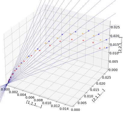
Figure 6: Orbits of the data from the quantum advantage experiment with Borealis. In red Borealis data, in blue and orange the simulated data from the thermal and squashed sampler respectively. The size of the sample was $\sim 10^{6}$. The points correspond to the number of detected photons from 18 (from the right) to 32 (to the left). The Borealis data are those of Fig. 3a of Ref. [5]. The lines are those we obtained from the thermal simulations in Figure 4

References

- Arute et al. [2019] F. Arute, K. Arya, R. Babbush, D. Bacon, J. C. Bardin, R. Barends, R. Biswas, S. Boixo, F. G. S. L. Brandao, D. A. Buell, and et al., Quantum supremacy using a programmable superconducting processor, Nature 574, 505–510 (2019).
- Zhong et al. [2020] H.-S. Zhong, H. Wang, Y.-H. Deng, M.-C. Chen, L.-C. Peng, Y.-H. Luo, J. Qin, D. Wu, X. Ding, Y. Hu, P. Hu, X.-Y. Yang, W.-J. Zhang, H. Li, Y. Li, X. Jiang, L. Gan, G. Yang, L. You, Z. Wang, L. Li, N.-L. Liu, C.-Y. Lu, and J.-W. Pan, Quantum computational advantage using photons, Science 370, 1460 (2020).
- Wu et al. [2021] Y. Wu, W.-S. Bao, S. Cao, F. Chen, M.-C. Chen, X. Chen, T.-H. Chung, H. Deng, Y. Du, D. Fan, M. Gong, C. Guo, C. Guo, S. Guo, L. Han, L. Hong, H.-L. Huang, Y.-H. Huo, L. Li, N. Li, S. Li, Y. Li, F. Liang, C. Lin, J. Lin, H. Qian, D. Qiao, H. Rong, H. Su, L. Sun, L. Wang, S. Wang, D. Wu, Y. Xu, K. Yan, W. Yang, Y. Yang, Y. Ye, J. Yin, C. Ying, J. Yu, C. Zha, C. Zhang, H. Zhang, K. Zhang, Y. Zhang, H. Zhao, Y. Zhao, L. Zhou, Q. Zhu, C.-Y. Lu, C.-Z. Peng, X. Zhu, and J.-W. Pan, Strong quantum computational advantage using a superconducting quantum processor, Phys. Rev. Lett. 127, 180501 (2021).
- Zhong et al. [2021] H.-S. Zhong, Y.-H. Deng, J. Qin, H. Wang, M.-C. Chen, L.-C. Peng, Y.-H. Luo, D. Wu, S.-Q. Gong, H. Su, Y. Hu, P. Hu, X.-Y. Yang, W.-J. Zhang, H. Li, Y. Li, X. Jiang, L. Gan, G. Yang, L. You, Z. Wang, L. Li, N.-L. Liu, J. J. Renema, C.-Y. Lu, and J.-W. Pan, Phase-programmable gaussian boson sampling using stimulated squeezed light, Phys. Rev. Lett. 127, 180502 (2021).
- Madsen et al. [2022] L. S. Madsen, F. Laudenbach, M. Falamarzi.Askarani, F. Rortais, T. Vincent, J. F. F. Bulmer, F. M. Miatto, L. Neuhaus, L. G. Helt, M. J. Collins, A. E. Lita, T. Gerrits, S. W. Nam, V. D. Vaidya, M. Menotti, I. Dhand, Z. Vernon, N. Quesada, and J. Lavoie, Quantum computational advantage with a programmable photonic processor, Nature 606, 75 (2022).
- Deng et al. [2023a] Y.-H. Deng, Y.-C. Gu, H.-L. Liu, S.-Q. Gong, H. Su, Z.-J. Zhang, H.-Y. Tang, M.-H. Jia, J.-M. Xu, M.-C. Chen, H.-S. Zhong, J. Qin, H. Wang, L.-C. Peng, J. Yan, Y. Hu, J. Huang, H. Li, Y. Li, Y. Chen, X. Jiang, L. Gan, G. Yang, L. You, L. Li, N.-L. Liu, J. J. Renema, C.-Y. Lu, and J.-W. Pan, Gaussian boson sampling with pseudo-photon-number resolving detectors and quantum computational advantage (2023a), arXiv:2304.12240 [quant-ph] .
- Preskill [2018] J. Preskill, Quantum computing in the nisq era and beyond, Quantum 2, 79 (2018).
- Aaronson and Arkhipov [2011] S. Aaronson and A. Arkhipov, The computational complexity of linear optics, in Proceedings of the forty-third annual ACM symposium on Theory of computing (ACM, 2011).
- Brod et al. [2019] D. J. Brod, E. F. Galvão, A. Crespi, R. Osellame, N. Spagnolo, and F. Sciarrino, Photonic implementation of boson sampling: a review, Advanced Photonics 1, 034001 (2019).
- Lund et al. [2014] A. Lund, A. Laing, S. Rahimi-Keshari, T. Rudolph, J. O’Brien, and T. Ralph, Boson sampling from a gaussian state, Physical Review Letters 113, 100502 (2014).
- Hamilton et al. [2017] C. S. Hamilton, R. Kruse, L. Sansoni, S. Barkhofen, C. Silberhorn, and I. Jex, Gaussian boson sampling, Physical Review Letters 119, 170501 (2017).
- Deshpande et al. [2022] A. Deshpande, A. Mehta, T. Vincent, N. Quesada, M. Hinsche, M. Ioannou, L. Madsen, J. Lavoie, H. Qi, J. Eisert, D. Hangleiter, B. Fefferman, and I. Dhand, Quantum computational advantage via high-dimensional gaussian boson sampling, Science Advances 8, eabi7894 (2022).
- Bromley et al. [2020] T. R. Bromley, J. M. Arrazola, S. Jahangiri, J. Izaac, N. Quesada, A. D. Gran, M. Schuld, J. Swinarton, Z. Zabaneh, and N. Killoran, Applications of near-term photonic quantum computers: software and algorithms, Quantum Science and Technology 5, 034010 (2020).
- Arrazola and Bromley [2018] J. M. Arrazola and T. R. Bromley, Using gaussian boson sampling to find dense subgraphs, Physical Review Letters 121, 030503 (2018).
- Schuld et al. [2020] M. Schuld, K. Brádler, R. Israel, D. Su, and B. Gupt, Measuring the similarity of graphs with a gaussian boson sampler, Physical Review A 101, 032314 (2020).
- Brádler et al. [2021] K. Brádler, S. Friedland, J. Izaac, N. Killoran, and D. Su, Graph isomorphism and gaussian boson sampling, Special Matrices 9, 166 (2021).
- Arrazola et al. [2021] J. M. Arrazola, V. Bergholm, K. Brádler, T. R. Bromley, M. J. Collins, I. Dhand, A. Fumagalli, T. Gerrits, A. Goussev, L. G. Helt, J. Hundal, T. Isacsson, R. B. Israel, J. Izaac, S. Jahangiri, R. Janik, N. Killoran, S. P. Kumar, J. Lavoie, A. E. Lita, D. H. Mahler, M. Menotti, B. Morrison, S. W. Nam, L. Neuhaus, H. Y. Qi, N. Quesada, A. Repingon, K. K. Sabapathy, M. Schuld, D. Su, J. Swinarton, A. Száva, K. Tan, P. Tan, V. D. Vaidya, Z. Vernon, Z. Zabaneh, and Y. Zhang, Quantum circuits with many photons on a programmable nanophotonic chip, Nature 591, 54 (2021).
- Sempere-Llagostera et al. [2022] S. Sempere-Llagostera, R. B. Patel, I. A. Walmsley, and W. S. Kolthammer, Experimentally finding dense subgraphs using a time-bin encoded gaussian boson sampling device, Phys. Rev. X 12, 031045 (2022).
- Yu et al. [2023] S. Yu, Z.-P. Zhong, Y. Fang, R. B. Patel, Q.-P. Li, W. Liu, Z. Li, L. Xu, S. Sagona-Stophel, E. Mer, S. E. Thomas, Y. Meng, Z.-P. Li, Y.-Z. Yang, Z.-A. Wang, N.-J. Guo, W.-H. Zhang, G. K. Tranmer, Y. Dong, Y.-T. Wang, J.-S. Tang, C.-F. Li, I. A. Walmsley, and G.-C. Guo, A universal programmable gaussian boson sampler for drug discovery (2023), arXiv:2210.14877 [quant-ph] .
- Deng et al. [2023b] Y.-H. Deng, S.-Q. Gong, Y.-C. Gu, Z.-J. Zhang, H.-L. Liu, H. Su, H.-Y. Tang, J.-M. Xu, M.-H. Jia, M.-C. Chen, H.-S. Zhong, H. Wang, J. Yan, Y. Hu, J. Huang, W.-J. Zhang, H. Li, X. Jiang, L. You, Z. Wang, L. Li, N.-L. Liu, C.-Y. Lu, and J.-W. Pan, Solving graph problems using gaussian boson sampling, Phys. Rev. Lett. 130, 190601 (2023b).
- Clifford and Clifford [2017] P. Clifford and R. Clifford, The classical complexity of boson sampling (2017), arXiv:1706.01260 [cs.DS] .
- Neville et al. [2017] A. Neville, C. Sparrow, R. Clifford, E. Johnston, P. M. Birchall, A. Montanaro, and A. Laing, Classical boson sampling algorithms with superior performance to near-term experiments, Nature Physics 13, 1153 (2017).
- Quesada and Arrazola [2020] N. Quesada and J. M. Arrazola, Exact simulation of gaussian boson sampling in polynomial space and exponential time, Phys. Rev. Research 2, 023005 (2020).
- Quesada et al. [2022] N. Quesada, R. S. Chadwick, B. A. Bell, J. M. Arrazola, T. Vincent, H. Qi, and R. GarcíaPatrón, Quadratic speed-up for simulating gaussian boson sampling, PRX Quantum 3, 010306 (2022).
- Oh et al. [2022] C. Oh, Y. Lim, B. Fefferman, and L. Jiang, Classical simulation of boson sampling based on graph structure (2022), arXiv:2110.01564 [quant-ph] .
- Bulmer et al. [2022] J. F. F. Bulmer, B. A. Bell, R. S. Chadwick, A. E. Jones, D. Moise, A. Rigazzi, J. Thorbecke, U.-U. Haus, T. V. Vaerenbergh, R. B. Patel, I. A. Walmsley, and A. Laing, The boundary for quantum advantage in gaussian boson sampling, Science Advances 8, eabl9236 (2022).
- Drummond et al. [2022] P. D. Drummond, B. Opanchuk, A. Dellios, and M. D. Reid, Simulating complex networks in phase space: Gaussian boson sampling, Phys. Rev. A 105, 012427 (2022).
- Popova and Rubtsov [2021] A. S. Popova and A. N. Rubtsov, Cracking the quantum advantage threshold for gaussian boson sampling (2021), arXiv:2106.01445 [quant-ph] .
- Cilluffo et al. [2023] D. Cilluffo, N. Lorenzoni, and M. B. Plenio, Simulating gaussian boson sampling with tensor networks in the heisenberg picture (2023), arXiv:2305.11215 [quant-ph] .
- Oh et al. [2023a] C. Oh, M. Liu, Y. Alexeev, B. Fefferman, and L. Jiang, Tensor network algorithm for simulating experimental gaussian boson sampling (2023a), arXiv:2306.03709 [quant-ph] .
- Rahimi-Keshari et al. [2016] S. Rahimi-Keshari, T. C. Ralph, and C. M. Caves, Sufficient conditions for efficient classical simulation of quantum optics, Phys. Rev. X 6, 021039 (2016).
- Oszmaniec and Brod [2018] M. Oszmaniec and D. J. Brod, Classical simulation of photonic linear optics with lost particles, New Journal of Physics 20, 092002 (2018).
- García-Patrón et al. [2019] R. García-Patrón, J. J. Renema, and V. Shchesnovich, Simulating boson sampling in lossy architectures, Quantum 3, 169 (2019).
- Brod and Oszmaniec [2020] D. J. Brod and M. Oszmaniec, Classical simulation of linear optics subject to nonuniform losses, Quantum 4, 267 (2020).
- Qi et al. [2020] H. Qi, D. J. Brod, N. Quesada, and R. García-Patrón, Regimes of classical simulability for noisy gaussian boson sampling, Phys. Rev. Lett. 124, 100502 (2020).
- Oh et al. [2021] C. Oh, K. Noh, B. Fefferman, and L. Jiang, Classical simulation of lossy boson sampling using matrix product operators, Phys. Rev. A 104, 022407 (2021).
- Liu et al. [2023] M. Liu, C. Oh, J. Liu, L. Jiang, and Y. Alexeev, Complexity of gaussian boson sampling with tensor networks (2023), arXiv:2301.12814 [quant-ph] .
- Renema et al. [2018] J. J. Renema, A. Menssen, W. R. Clements, G. Triginer, W. S. Kolthammer, and I. A. Walmsley, Efficient classical algorithm for boson sampling with partially distinguishable photons, Phys. Rev. Lett. 120, 220502 (2018).
- Moylett et al. [2019] A. E. Moylett, R. García-Patrón, J. J. Renema, and P. S. Turner, Classically simulating near-term partially-distinguishable and lossy boson sampling, Quantum Science and Technology 5, 015001 (2019).
- Renema [2020a] J. J. Renema, Simulability of partially distinguishable superposition and gaussian boson sampling, Phys. Rev. A 101, 063840 (2020a).
- Shi and Byrnes [2022] J. Shi and T. Byrnes, Effect of partial distinguishability on quantum supremacy in gaussian boson sampling, npj Quantum Information 8, 54 (2022).
- Spagnolo et al. [2014] N. Spagnolo, C. Vitelli, M. Bentivegna, D. J. Brod, A. Crespi, F. Flamini, S. Giacomini, G. Milani, R. Ramponi, P. Mataloni, R. Osellame, E. F. Galvão, and F. Sciarrino, Experimental validation of photonic boson sampling, Nature Photonics 8, 615 (2014).
- Martínez-Cifuentes et al. [2022] J. Martínez-Cifuentes, K. M. Fonseca-Romero, and N. Quesada, Classical models are a better explanation of the jiuzhang 1.0 gaussian boson sampler than its targeted squeezed light model (2022), arXiv:2207.10058 [quant-ph] .
- Walschaers et al. [2016] M. Walschaers, J. Kuipers, J.-D. Urbina, K. Mayer, M. C. Tichy, K. Richter, and A. Buchleitner, Statistical benchmark for BosonSampling, New Journal of Physics 18, 032001 (2016).
- Phillips et al. [2019] D. S. Phillips, M. Walschaers, J. J. Renema, I. A. Walmsley, N. Treps, and J. Sperling, Benchmarking of gaussian boson sampling using two-point correlators, Phys. Rev. A 99, 023836 (2019).
- Giordani et al. [2018] T. Giordani, F. Flamini, M. Pompili, N. Viggianiello, N. Spagnolo, A. Crespi, R. Osellame, N. Wiebe, M. Walschaers, A. Buchleitner, and F. Sciarrino, Experimental statistical signature of many-body quantum interference, Nature Photonics 12, 173 (2018).
- Renema [2020b] J. J. Renema, Marginal probabilities in boson samplers with arbitrary input states (2020b), arXiv:2012.14917 [quant-ph] .
- Villalonga et al. [2021] B. Villalonga, M. Y. Niu, L. Li, H. Neven, J. C. Platt, V. N. Smelyanskiy, and S. Boixo, Efficient approximation of experimental gaussian boson sampling (2021), arXiv:2109.11525 [quant-ph] .
- Giordani et al. [2022] T. Giordani, V. Mannucci, N. Spagnolo, M. Fumero, A. Rampini, E. Rodolà, and F. Sciarrino, Certification of gaussian boson sampling via graphs feature vectors and kernels, Quantum Science and Technology 8, 015005 (2022).
- Xanadu [2023] Xanadu, Xanadu Cloud (2023).
- Amazon Web Services [2020] Amazon Web Services, Amazon Braket (2020).
- Goldberg et al. [2023] A. Z. Goldberg, G. S. Thekkadath, and K. Heshami, Measuring the quadrature coherence scale on a cloud quantum computer, Phys. Rev. A 107, 042610 (2023).
- [53] Operating borealis — advanced, https://strawberryfields.ai/photonics/demos/tutorial_borealis_advanced.html, accessed: 2023-04-17.
- Takeda and Furusawa [2019] S. Takeda and A. Furusawa, Toward large-scale fault-tolerant universal photonic quantum computing, APL Photonics 4, 060902 (2019).
- Motes et al. [2014] K. R. Motes, A. Gilchrist, J. P. Dowling, and P. P. Rohde, Scalable boson sampling with time-bin encoding using a loop-based architecture, Phys. Rev. Lett. 113, 120501 (2014).
- He et al. [2017] Y. He, X. Ding, Z.-E. Su, H.-L. Huang, J. Qin, C. Wang, S. Unsleber, C. Chen, H. Wang, Y.-M. He, X.-L. Wang, W.-J. Zhang, S.-J. Chen, C. Schneider, M. Kamp, L.-X. You, Z. Wang, S. Höfling, C.-Y. Lu, and J.-W. Pan, Time-bin-encoded boson sampling with a single-photon device, Phys. Rev. Lett. 118, 190501 (2017).
- Van Rossum and Drake [2009] G. Van Rossum and F. L. Drake, Python 3 Reference Manual (CreateSpace, Scotts Valley, CA, 2009).
- Killoran et al. [2019] N. Killoran, J. Izaac, N. Quesada, V. Bergholm, M. Amy, and C. Weedbrook, Strawberry Fields: A software platform for photonic quantum computing, Quantum 3, 129 (2019).
- Gupt et al. [2019] B. Gupt, J. Izaac, and N. Quesada, The walrus: a library for the calculation of hafnians, hermite polynomials and gaussian boson sampling, Journal of Open Source Software 4, 1705 (2019).
- Jahangiri et al. [2020] S. Jahangiri, J. M. Arrazola, N. Quesada, and N. Killoran, Point processes with gaussian boson sampling, Phys. Rev. E 101, 022134 (2020).
- Rahimi-Keshari et al. [2015] S. Rahimi-Keshari, A. P. Lund, and T. C. Ralph, What can quantum optics say about computational complexity theory?, Phys. Rev. Lett. 114, 060501 (2015).
- Oh et al. [2023b] C. Oh, B. Fefferman, L. Jiang, and N. Quesada, Quantum-inspired classical algorithm for graph problems by gaussian boson sampling (2023b), arXiv:2302.00536 [quant-ph] .
- Solomons et al. [2023] N. R. Solomons, O. F. Thomas, and D. P. S. McCutcheon, Gaussian-boson-sampling-enhanced dense subgraph finding shows limited advantage over efficient classical algorithms (2023), arXiv:2301.13217 [quant-ph] .