Modile as a conservative tail risk measurer: the solution of an optimisation problem with 0-1 loss function

Abstract

Quantiles and expectiles, which are two important concepts and tools in tail risk measurements, can be regarded as an extension of median and mean, respectively. Both of these tail risk measurers can actually be embedded in a common framework of $L_{p}$ optimization with the absolute loss function ($p=1$) and quadratic loss function ($p=2$), respectively. When 0-1 loss function is frequently used in statistics, machine learning and decision theory, this paper introduces an 0-1 loss function based $L_{0}$ optimisation problem for tail risk measure and names its solution as modile, which can be regarded as an extension of mode. Mode, as another measure of central tendency, is more robust than expectiles with outliers and easy to compute than quantiles. However, mode based extension for tail risk measure is new. This paper shows that the proposed modiles are not only more conservative than quantiles and expectiles for skewed and heavy-tailed distributions, but also providing or including the unique interpretation of these measures. Further, the modiles can be regarded as a type of generalized quantiles and doubly truncated tail measure whcih have recently attracted a lot of attention in the literature. The asymptotic properties of the corresponding sample-based estimators of modiles are provided, which, together with numerical analysis results, show that the proposed modiles are promising for tail measurement.

1 Introduction

Quantile (Koenker and Bassett, 1978) and expectile (Newey and Powell, 1987) have been attracted considerable attention in the literature with wide application in statistics, economics, finance and risk management, see Breckling and Chambers (1988), Waltrup et al. (2015), Ehm et al. (2016), Daouia et al. (2018), Daouia et al. (2019), Madrid Padilla and Chatterjee (2022), Dimitriadis and Halbleib (2022), Dimitriadis et al. (2022) and among others.

For $\tau\in(0,1)$, the $\tau$th quantile $q_{\tau}$ of a random variable $Y$ can be regarded as a skew modification of median as it minimises an asymmetric absolute loss function:

$$\begin{split}q_{\tau}=\arg\min_{\theta\in\mathbb{R}}\text{E}\left\{\left|\tau-I(Y\leq\theta)\right|\cdot|Y-\theta|\right\}.\end{split}$$ (1.1)

This is, $q_{\tau}$ is the solution of a $L_{1}$ optimisation problem. When $\tau=1/2$, the quantile of $Y$ reduces to its mean.

The $\tau$th expectile $\xi_{\tau}$ of a random variable $Y$ can be regarded as a skew modification of mean as it minimises an asymmetric quadratic loss function:

$$\xi_{\tau}=\arg\min_{\theta\in\mathbb{R}}\text{E}\left\{|\tau-I(Y\leq\theta)|\cdot(Y-\theta)^{2}\right\}.$$ (1.2)

This is, $\xi_{\tau}$ is the solution of a $L_{2}$ optimisation problem. When $\tau=1/2$, the expectile of $Y$ reduces to its mean. Note that $q_{\tau}$ equivalently ((Newey and Powell, 1987)) satisfies

$$\frac{P(Y\geq q_{\tau})}{P(Y<q_{\tau})}=\frac{1-F_{Y}(q_{\tau})}{F_{Y}(q_{\tau})}=\frac{1-\tau}{\tau},$$ (1.3)

and $\xi_{\tau}$ equivalently satisfies

$$\frac{\int_{\xi_{\tau}}^{+\infty}(y-\xi_{\tau})\,dF_{Y}(y)}{\int_{-\infty}^{\xi_{\tau}}(\xi_{\tau}-y)\,dF_{Y}(y)}=\frac{E(Y-\xi_{\tau})_{+}}{E(Y-\xi_{\tau})_{-}}=\frac{1-\tau}{\tau},$$ (1.4)

where $F_{Y}(\cdot)$ is the cumulative distribution function (cdf) of a random variable $Y$. Here $(1-\tau)/{\tau}$ is the targeted probability ratio and the expectile level ratio or targeted gain-loss ratio for (1.3) and (1.4), respectively.

Mode (Parzen, 1962), as another most important characteristic of a random variable, usually represents the value where probability density is the biggest for a continuous random variable, and the most probable value for a discrete random variable but links to tail risk measure rarely. However, based on an optimisation problem with an 0-1 loss function, this paper introduces a new tail risk measurement, which can be an extension of mode and include the unique interpretation of both quantiles and expectiles.

The remainder of this paper is organized as follows. In Section 2, the definition of modile is proposed. Section 3 shows that modiles are more conservative than the popular quantiles and expectiles for skewed and heavy-tailed distributions. The estimation algorithm and asymptotic property of modiles are developed in Section 4. Both simulation examples and the application of modiles on real data are given in Section 5. Some technical proofs are provided in the Appendix.

2 The Modile and its basic properties

Note that the mode $\nu$ of a random variable $Y$ could be defined in terms of the $L_{0}$ optimisation problem $\nu=\arg\min_{\theta\in\mathbb{R}}\text{E}\left\{L(Y,\theta)\right\}$ with the 0-1 loss unction $L(Y,\theta)=I(|Y-\theta|>\delta)$. Where $\delta>0$ is a constant. See (Lee, 1989, 1993) and among others.

Also note that the defined mode above often requires the density function $f_{Y}(y)$ of $Y$ is strictly unimodal. To relax the restriction and include non-monotone density, asymmetric density and even multi-modual, we may consider an alternative 0-1 loss function with a lower limit $-h_{1}$ and upper limit $h_{2}$ and then formulate the $L_{0}$ optimisation problem as

$$\nu=\arg\min_{\nu\in\mathbb{R}}\text{E}\{I(-h_{1}\leq Y-\theta\leq h_{2})\}.$$

In fact, this 0-1 loss function should define $\nu$ as the mode of the random variable $Y$ (Ho et al., 2017). When $h_{1}=h_{2}$ and $\tau=0.5$, modile (2.1) is equal to mode (Lee, 1989).

Then, along the same line of defining quantiles and expectiles as the optimal predictors under an asymmetric absolute loss function and asymmetric least squares loss function respectively, we define the modile as an asymmetric 0-1 loss function based $L_{0}$ optimisation as:

$$\begin{split}\nu_{\tau}=\arg\max_{\theta\in\mathbb{R}}\text{E}\left\{|\tau-I(Y\leq\theta)|\cdot I(-h_{1}\leq Y-\theta\leq h_{2})\right\}\end{split}$$ (2.1)

or

$$\begin{split}\nu_{\tau}=\arg\min_{\theta\in\mathbb{R}}\text{E}\left[|\tau-I(Y\leq\theta)|\cdot\left\{I(Y-\theta<-h_{1})+I(Y-\theta>h_{2})\right\}\right],\end{split}$$ (2.2)

for two fixed positive number $h_{1}$ and $h_{2}$. That is, $\nu_{\tau}$ is defined as the $\tau$th modile of a random variable $Y$ for any $0<\tau<1$. Based on the equations (2.1) or (2.2), we have

$$\begin{split}\text{E}\left\{\rho_{\tau}(Y-\nu_{\tau},h_{1},h_{2})\right\}=&\tau\,P(Y>\nu_{\tau}+h_{2})+(1-\tau)\,P(Y<\nu_{\tau}-h_{1})\\ =&\tau-\tau\,F_{Y}(\nu_{\tau}+h_{2})+(1-\tau)\,F_{Y}(\nu_{\tau}-h_{1}),\end{split}$$

where

$$\rho_{\tau}(u,h_{1},h_{2})=|\tau-I(u<0)|\cdot\left\{I(u<-h_{1})+I(u>h_{2})\right\}=\begin{cases}\tau,&\text{if }u>h_{2}\\ 1-\tau,&\text{if }u<-h_{1}\\ 0,&\text{otherwise. }\end{cases}$$

So, we have

$$\begin{split}\frac{d\,E\rho_{\tau}(Y-\nu_{\tau},h_{1},h_{2})}{d\,\nu_{\tau}}=-\tau\,f_{Y}(\nu_{\tau}+h_{2})+(1-\tau)\,f_{Y}(\nu_{\tau}-h_{1})=0,\end{split}$$ (2.3)

where $f_{Y}(\cdot)$ is the probability density function (pdf) of a random variable $Y$. We obtain

$$\frac{f_{Y}(\nu_{\tau}+h_{2})}{f_{Y}(\nu_{\tau}-h_{1})}=\frac{1-\tau}{\tau}.$$ (2.4)

Here $f_{Y}(\nu_{\tau}+h_{2})$ and $f_{Y}(\nu_{\tau}-h_{1})$ can be interpreted as the most likely gain and most likely loss of $Y$, respectively.

In the following, in some special cases of $f_{Y}(\cdot)$, let’s specify the modile $\nu_{\tau}$ via (2.4).

(1) If $Y\sim Normal(\mu,\sigma^{2})$, we have $\nu_{\tau}=\mu+\frac{h_{1}-h_{2}}{2}-\frac{\sigma^{2}}{h_{1}+h_{2}}\ln\left(\frac{1-\tau}{\tau}\right)$. Let $h_{1}=h_{2}$, then $\nu_{\tau}=\mu$ ($\mu$ is the mode) under $\tau=0.5$.

(2) If $Y\sim Laplace(\mu,\lambda)$, $\nu_{\tau}=\mu+(h_{1}-h_{2})/2-\frac{\lambda}{2}\ln\left(\frac{1-\tau}{\tau}\right)$ for $\min\{h_{1},h_{2}\}\geq|\nu_{\tau}-\mu|$. If $h_{1}=h_{2}$, $\nu_{\tau}=\mu$ ($\mu$ is the mode) under $\tau=0.5$.

(3) If $Y\sim Gamma(\alpha,\beta)$, its density function is $f(x)=\frac{\beta^{\alpha}}{\Gamma(\alpha)}x^{\alpha-1}e^{-\beta x}$ with $x\geq 0,\alpha>0,\beta>0$. We have $\nu_{\tau}=(Ah_{1}+h_{2})/(A-1)$, where $A=\frac{1-\tau}{\tau}\exp\{\frac{\beta}{\alpha-1}(h_{1}+h_{2})\}$. When $h_{1}$ and $h_{2}$ satisfy $h_{1}+h_{2}=B\ln\left(\frac{B+h_{2}}{B-h_{1}}\right),$ where $B=(\alpha-1)/\beta$ is the mode, then $\nu_{\tau}=B$ under $\tau=0.5$.

(4) If $f_{Y}(x)=12(b-a)^{3}\cdot(x-\frac{a+b}{2})^{2}\cdot I(a\leq x\leq b)$, the mode is $a$ and $b$, we have $\nu_{\tau}=\left\{{\frac{a+b}{2}-h_{2}+(\frac{a+b}{2}+h_{1})A}\right\}/(1+A),$ where $A=\pm\sqrt{\frac{1-\tau}{\tau}}$. When $\tau=0.5$, $\nu_{\tau}=(a+b-h_{2}+h_{1})/2=a$ (or $b$) under $h_{1}=a$, $h_{2}=b$ (or $h_{1}=b$, $h_{2}=a$).

In the above examples, the modile $\nu_{\tau}$ has a close-form expression under some density functions. Moreover, mode is a special case of modile for symmetrically distributed loss particularly when $h_{1}=h_{2}$. In the following example, we set $h_{1}=a+|b-c|$ and $h_{2}=a+|b+c|$, where $a,b,c$ are standard deviation, mean and skewness of data, respectively. The numberical results of the quantiles, expectiles and modiles for Normal distribution, Laplace distribution and Gamma distribution are shown in Table 1 and Figures 1-3.

Table 1: The modile, quantile and expectile under different errors and $\tau$s.

$\bm{Y}$		Normal(0,1)			Laplace(1,2)			Gamma(8,7)
$\tau$	modile	quantile	expectile	modile	quantile	expectile	modile	quantile	expectile
0.1	-1.099	-1.282	-0.861	-1.197	-2.219	-1.404	0.855	0.665	0.833
0.2	-0.693	-0.842	-0.549	-0.386	-0.833	-0.452	0.875	0.797	0.938
0.3	-0.424	-0.524	-0.337	0.153	-0.022	0.135	0.901	0.902	1.014
0.4	-0.203	-0.253	-0.162	0.595	0.554	0.592	0.936	0.999	1.080
0.5	0.000	0.000	0.000	1.000	1.000	1.000	0.987	1.096	1.143
0.6	0.203	0.253	0.162	1.405	1.446	1.408	1.066	1.199	1.209
0.7	0.424	0.524	0.337	1.847	2.022	1.865	1.206	1.316	1.283
0.8	0.693	0.842	0.549	2.386	2.833	2.452	1.525	1.462	1.377
0.9	1.099	1.282	0.861	3.197	4.219	3.404	2.972	1.682	1.523

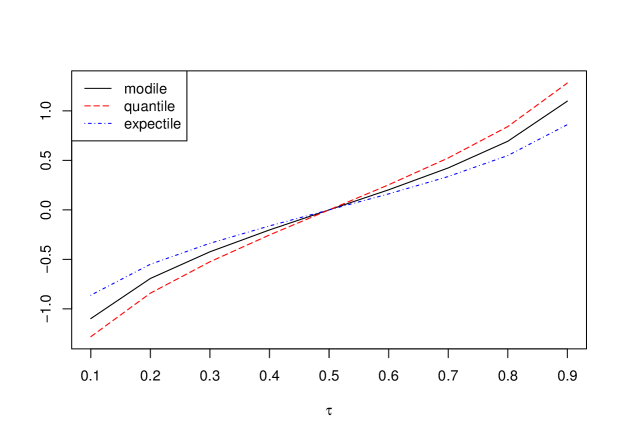
Figure 1: The modile, quantile and expectile for $\bm{Y}\sim$Normal(0,1).

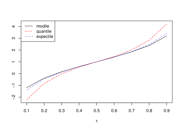
Figure 2: The modile, quantile and expectile for $\bm{Y}\sim$Laplace(1,2).

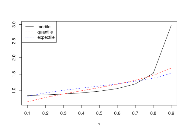
Figure 3: The modile, quantile and expectile for $\bm{Y}\sim$Gamma(8,7).

Theorem 1. Let $\delta=h_{1}=h_{2}\equiv\delta$, for any $x\in(0,\delta)$, the $\nu_{\tau}$ satisfies that

$$\frac{f_{Y}(\nu_{\tau}+x)}{f_{Y}(\nu_{\tau}-x)}=\frac{1-\tau}{\tau}.$$ (2.5)

Then for any $\delta$, the following equation holds:

$$\begin{split}\frac{P(\nu_{\tau}\leq Y\leq\nu_{\tau}+\delta)}{P(\nu_{\tau}-\delta\leq Y\leq\nu_{\tau})}=\frac{1-\tau}{\tau},\end{split}$$ (2.6)

and

$$\frac{E\{(Y-\nu_{\tau})\,I(\nu_{\tau}\leq Y\leq\nu_{\tau}+\delta)\}}{E\{(\nu_{\tau}-Y)\,I(\nu_{\tau}-\delta\leq Y\leq\nu_{\tau})\}}=\frac{1-\tau}{\tau}.$$ (2.7)

When $\delta\rightarrow\infty$, we have

$$\frac{P(Y\geq\nu_{\tau})}{P(Y\leq\nu_{\tau})}=\frac{1-\tau}{\tau},$$ (2.8)

and

$$\frac{E\{(Y-\nu_{\tau})\,I(Y\geq\nu_{\tau})\}}{E\{(\nu_{\tau}-Y)\,I(Y\leq\nu_{\tau})\}}=\frac{1-\tau}{\tau}.$$ (2.9)

Theorem 1 shows that modile of $Y$ are determined by its tail range (interval) probabilities. The left side of the equation (2.6) can be interpreted as the probability ratio of the ranges of gain and loss, and the right side $(1-\tau)/{\tau}$ is the targeted most-likely gain-loss range ratio. (2.8) shows that quantiles are the special cases of modile. Furthermore, we have the expectations of the tail range of $Y$ in (2.6), and the expectiles of $Y$ are also the special cases of modile as when $\delta\rightarrow\infty$ in (2.8).

Remark 1: For any $\tau\in(0,1)$, the following density function $f_{Y}(\cdot)$ satisfies the condition (2.5),

$$f_{Y}(x)=\begin{cases}~{}2(1-\tau)f(x),&\text{if }x\geq\nu\\ \ 2\tau f(x),&\text{if }x<\nu,\end{cases}$$

where $f(\cdot)$ is a symmetric density function and $\nu$ is the mode of $f(\cdot)$. $f_{Y}(\cdot)$ is a function of $\tau$ because we make $\nu_{\tau}=\nu$.

For example, $f(\cdot)$ is the density function of standard Normal distribution, then $\nu=\nu_{\tau}=0$. We have

$$f_{Y}(x)=\begin{cases}\frac{2(1-\tau)}{\sqrt{2\pi}}\exp(-x^{2}/2),&\text{if }x\geq 0\\ \ \frac{2\tau}{\sqrt{2\pi}}\exp(-x^{2}/2),&\text{if }x<0,\end{cases}$$

satisfies the condition (2.4), and $\nu_{\tau}=q_{\tau}=\xi_{\tau}$.

Remark 2: Note that we may re-write modiles as the minimizer of

$$\nu_{\tau}=\arg\min_{\theta\in\mathbb{R}}\left[\tau\text{E}\{\Phi_{1}((Y-\theta)^{+})\}+(1-\tau)\text{E}\{\Phi_{2}((Y-\theta)^{-})\}\right],$$

with convex loss function $\Phi_{1}(u)=I[u\leq Y\leq u+h_{2}]$ and $\Phi_{2}(u)=-I[u-h_{1}\leq Y\leq u]$, which is a type of Generalized quantiles defined in (Bellini et al., 2014) but without a need to satisfy the first-order condition of (Bellini et al., 2014). The convex of $\Phi_{i}(\cdot)$ ($i=1,2$) is due to the fact that the associated sets are convex.

Equations (2.6)-(2.7) show that the proposes modiles may also propose a type of doubly truncated tail probability, while the doubly truncated tail conditional expectation $\text{E}(X|x_{p}<X<x_{q})$ has recently attracted much attention in the literature ((Roozegar et al., 2020; Shushi and Yao, 2020)), where $x_{p}$ is the p-th quantile, and $0\leq p<q\leq 1.$

3 Conservative risk measure for skewed and heavy-tailed distributions

For most studies in risk management, it has been found that Pareto distribution, which is a skewed and heavy-tailed distribution, describe quite well of the tail structure of actuarial and financial data. Here we consider a Pareto distribution with shape parameter $\alpha\in(0,+\infty)$, which is a continuous distribution on $(1,+\infty)$ with distribution function $F$ given by $F(y)=1-y^{-\alpha}.$ The probability density function $f(y)$ is given by

$$f(y)=\alpha y^{-\alpha-1}.$$ (3.1)

From the equation (3.1), the $\tau$-th modile $\nu_{\tau}$ is

$$\nu_{\tau}=\frac{h_{1}+Ah_{2}}{1-A},$$ (3.2)

where $A=(1/\tau-1)^{\alpha+1}$.

It is easy to know that the quantile function of Pareto distribution is $q_{\tau}=(1-\tau)^{-1/\alpha}$. From the the result of Theorem 11 in Bellini et al. (2014), the expectile function of Pareto distribution is $\xi_{\tau}\approx\{(1-\tau)(\alpha-1)\}^{-1/\alpha}$ under $\alpha>1$ and $\tau\to 1$. Note that $\nu_{\tau}$ in (3.2), when $\tau\to 1$, we have $\nu_{\tau}=h_{1}<+\infty$, which is smaller than $q_{\tau}$ and $\xi_{\tau}$. Therefore, modile is a more conservative risk measure than the quantile and expectile.

Generally, for the Pareto-like with tail index $\alpha$ distribution

$$F(y)=1-L(y)y^{-\alpha}$$

for some function $L$ which is slowly varying at infinity. We consider the $\tau$th quantiles $q_{\tau}$ conditional on the modile-range $[\nu_{\tau}-h_{1},\,\,\nu_{\tau}+h_{2}]$:

$$\tau = P[Y<q_{\tau}|\nu_{\tau}-h_{1}\leq Y\leq\nu_{\tau}+h_{2}]$$

$$= \frac{(\nu_{\tau}-h_{1})^{-\alpha}-q_{\tau}^{-\alpha}}{(\nu_{\tau}-h_{1})^{-\alpha}-(\nu_{\tau}+h_{2})^{-\alpha}},$$

we have

$$q_{\tau}^{-\alpha}=\tau(\nu_{\tau}+h_{2})^{-\alpha}+(1-\tau)\,(\nu_{\tau}-h_{1})^{-\alpha}.$$

Clearly, for any $\alpha\in(0,+\infty)$, when $\tau\rightarrow 1$, $q_{\tau}=\nu_{\tau}+h_{2}>\nu_{\tau}$, and when $\tau\rightarrow 0$, $q_{\tau}=\nu_{\tau}-h_{1}<\nu_{\tau}$, so modiles are more generally conservative tail risk measures than quantiles.

Similar conclusion is true for expectiles. In fact, consider the $\tau$th expectiles $\xi_{\tau}$ conditional on the modile-range $[\nu_{\tau}-h_{1},\,\,\nu_{\tau}+h_{2}]$: from

$$\frac{E(Y-\xi_{\tau})_{+}}{E(Y-\xi_{\tau})_{-}}=\frac{\int_{\nu_{\tau}}^{\xi_{\tau}+h_{2}}(x-\xi_{\tau})\,dF(x)}{\int_{\nu_{\tau}-h_{1}}^{\xi_{\tau}}(\xi_{\tau}-x)\,dF(x)}=\frac{1-\tau}{\tau},$$

and

$$\int_{\nu_{\tau}-h_{1}}^{\xi_{\tau}}(\xi_{\tau}-x)\,dF(x) = \alpha\left\{\frac{\xi_{\tau}^{1-\alpha}-(\nu_{\tau}-h_{1})^{1-\alpha}}{1-\alpha}+\xi_{\tau}\cdot\frac{\xi_{\tau}^{-\alpha}-(\nu_{\tau}-h_{1})^{-\alpha}}{\alpha}\right\},$$

$$\int_{\nu_{\tau}}^{\xi_{\tau}+h_{2}}(x-\xi_{\tau})\,dF(x) = \alpha\left\{\frac{(\xi_{\tau}+h_{2})^{1-\alpha}-\xi_{\tau}^{1-\alpha}}{1-\alpha}+\xi_{\tau}\cdot\frac{(\xi_{\tau}+h_{2})^{-\alpha}-\xi_{\tau}^{-\alpha}}{\alpha}\right\},$$

under the Pareto-like heavy-tailed distribution, we have when $\tau\rightarrow 1$,

$$\alpha(\nu_{\tau}+h_{2})^{1-\alpha}+(1-\alpha)\xi(\nu_{\tau}+h_{2})^{-\alpha}=\xi_{\tau}^{1-\alpha},$$

which holds and only holds when $\xi_{\tau}=\nu_{\tau}+h_{2}$. Along the same derivation, we can show that when $\tau\rightarrow 0$, $\xi_{\tau}=\nu_{\tau}-h_{1}$.

4 Algorithm and asymptotic property of the estimation of modiles

Given a random sample $Y_{1},\ldots,Y_{n}$ from $Y$, the estimator of $\hat{\nu}_{\tau}$ of $\hat{\nu}_{\tau}$ $\hat{\nu}_{\tau}$ can be obtained by the minimisation of the empirical $L_{0}$ optimisation problem of the equation (2.2) under the 0-1 loss fcuntion as

$$\hat{\nu}_{\tau}=\arg\min_{\theta\in\mathbb{R}}\left\{\tau-\frac{\tau}{n}\sum^{n}_{i=1}I(Y_{i}\leq\theta+h_{2})+\frac{1-\tau}{n}\sum^{n}_{i=1}I(Y_{i}\leq\theta-h_{1})\right\}.$$ (4.1)

We can use the multitask algorithm (Qin et al., 2020) to find the numerical solutions of $\hat{\nu}_{\tau}$ easily. See the R code attached.

When the sample size $n$ tends to infty, the asymptotic distribution of $\hat{\nu}_{\tau}$ is given by Theorem 2.

Theorem 2. Assume that the density function of $Y$ is continuous differentiable, then we have

$$n^{1/3}(\hat{\nu}_{\tau}-\nu_{\tau})\xrightarrow{d}\left[\frac{4\tau f_{Y}(\nu_{\tau}+h_{2})}{\left\{\tau f^{\prime}_{Y}(\nu_{\tau}+h_{2})-(1-\tau)f^{\prime}_{Y}(\nu_{\tau}-h_{1})\right\}^{2}}\right]^{1/3}\hat{z},$$

where $\xrightarrow{d}$ stands for convergence in the distribution, $\hat{z}=\arg\max_{z\in\mathbb{R}}\{Z(z)-z^{2}\}$, and $Z(z)$ is a two-sided Wiener-Lévy process through the origin with mean 0 and variance one per unit $z$.

Note that the asymptotic distribution of $\hat{\nu}_{\tau}$ is the same as the estimation of the mode in Chernoff (1964) under $\tau=0.5$ and $h_{1}=h_{2}$.

5 Numerical studies

In this section, we first use Monte Carlo simulation studies to assess the finite sample performance of the proposed procedures and then demonstrate the application of the proposed methods with a real data analysis. All programs are written in R code.

5.1 Simulation example

In this section, we study the performance of the estimation of modile (E-modile) proposed in (4.1). We generate the sample size $n=10^{5}$ data of $Y$ from the following two distributions: Normal(0,1) and Laplace(1,2). The simulation results of sample E-modiles and absolute error (AE=$|\text{modile}-\text{E-modile}|$) based on $\tau=0.1,\ldots,0.9$ are shown in Table 2, which are based on 500 simulation replications. We can see from both Table 2 that the E-modile is very chose to modile in Table 1, thus the estimation method is valid.

Table 2: The means and standard deviations (in parentheses) of E-modile under different errors and $\tau$s for simulation example.

$\bm{Y}$	Normal(0,1)		Laplace(1,2)
$\tau$	E-modile	AE	E-modile	AE
0.1	-1.097 (0.034)	0.027 (0.020)	-1.197 (0.078)	0.064 (0.045)
0.2	-0.694 (0.026)	0.021 (0.016)	-0.384 (0.07)	0.055 (0.044)
0.3	-0.423 (0.024)	0.019 (0.015)	0.156 (0.068)	0.055 (0.040)
0.4	-0.202 (0.023)	0.019 (0.014)	0.591 (0.068)	0.055 (0.040)
0.5	-0.001 (0.022)	0.018 (0.013)	0.994 (0.070)	0.056 (0.041)
0.6	0.201 (0.022)	0.017 (0.013)	1.400 (0.068)	0.055 (0.040)
0.7	0.424 (0.024)	0.019 (0.014)	1.844 (0.072)	0.057 (0.043)
0.8	0.693 (0.026)	0.021 (0.015)	2.383 (0.069)	0.057 (0.039)
0.9	1.097 (0.033)	0.026 (0.019)	3.197 (0.078)	0.063 (0.047)

5.2 Real data example

To illustrate the practical usefulness of application of our proposed methods, a daily data of S&P500 index between January 4, 2010 and March 15, 2023 with 3321 observations in total. The data is downloaded from the website of Yahoo Finance (https://hk.finance.yahoo.com). The daily returns are computed as 100 times the difference of the log of the prices, that is, $Y_{t}=100\ln(p_{t}/p_{t-1})$, where $p_{t}$ is the daily price. Table 3 collects the summary statistics of $\{Y_{t}\}$, where the sample skewness 0.724 indicates possible asymmetries in the volatility, and the sample kurtosis 13.070 implies heavy tail of $\{Y_{t}\}$. Figure 4 also gives the time series plot for S&P500.

The sample modiles, quantiles and expectiles based on $\tau=0.1,\ldots,0.9$ are shown in Table 4 and Figure 5. The results show that modiles are the largest under small $\tau$ and smallest under large $\tau$ than quantiles and expectiles. This means that modile is more conservative than quantiles and expectiles.

Table 3: Summary statistics for S&P500 returns.

Mean	Median	std.Dev.	Skewness	Kurtosis	Min	Max
-0.037	-0.063	1.124	0.724	13.070	-8.97	12.765

Table 4: The sample modile, quantile and expectile under different errors and $\tau$s for real data example.

$\tau$	modile	quantile	expectile
0.1	-0.762	-1.177	-0.899
0.2	-0.562	-0.720	-0.561
0.3	-0.150	-0.439	-0.352
0.4	-0.063	-0.226	-0.187
0.5	0.105	0.063	-0.037
0.6	0.151	0.087	0.114
0.7	0.333	0.273	0.289
0.8	0.358	0.576	0.523
0.9	0.791	1.138	0.925

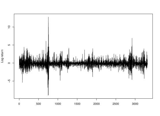
Figure 4: The time series plot of the daily return series between January 4, 2010 and March 15, 2023 .

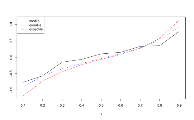
Figure 5: The modile, quantile and expectile for real data example.

6 Disussion

Modiles, as a new tail rik measure, have been introduced in this paper, which have their merits, giving existing it quantiles and expectiles tail risk measures. Like quantiles, modiles have a good interpretation and also include the unique interpretation of expectiles. Unlike quantiles, multivariate modiles should be well-defined along the same line as that of univariate case. They are worth further investigation in more details. The applications and their deep link to current double-truncated risk measures deserve to be studied further.

Appendix A Proof of main results

Proof of Theorem 1. From the condition ${f_{Y}(\nu_{\tau}+x)}/{f_{Y}(\nu_{\tau}-x)}=(1-\tau)/{\tau}$ for any $x\in(0,\delta)$, we have

$$\begin{split}P(\nu_{\tau}\leq Y\leq\nu_{\tau}+\delta)=&\int_{\nu_{\tau}}^{\nu_{\tau}+\delta}f_{Y}(t)\,dt=\int_{0}^{\delta}f_{Y}(\nu_{\tau}+t)\,dt\\ =&\frac{1-\tau}{\tau}\int_{0}^{\delta}f_{Y}(\nu_{\tau}-t)\,dt=\frac{1-\tau}{\tau}\int_{\nu_{\tau}-\delta}^{\nu_{\tau}}f_{Y}(t)\,dt\\ =&\frac{1-\tau}{\tau}P(\nu_{\tau}-\delta\leq Y\leq\nu_{\tau}),\end{split}$$

and

$$\begin{split}&E\{(Y-\nu_{\tau})\,I(\nu_{\tau}\leq Y\leq\nu_{\tau}+\delta)\}\\ =&\int_{\nu_{\tau}}^{\nu_{\tau}+\delta}(t-\nu_{\tau})f_{Y}(t)\,dt=\int_{0}^{\delta}tf_{Y}(\nu_{\tau}+t)\,dt\\ =&\frac{1-\tau}{\tau}\int_{0}^{\delta}tf_{Y}(\nu_{\tau}-t)\,dt=\frac{1-\tau}{\tau}\int_{\nu_{\tau}-\delta}^{\nu_{\tau}}(\nu_{\tau}-t)f_{Y}(t)\,dt\\ =&\frac{1-\tau}{\tau}E\{(\nu_{\tau}-Y)\,I(\nu_{\tau}-\delta\leq Y\leq\nu_{\tau})\}.\end{split}$$

Proof of Theorem 2. Note that (4.1), $\hat{\nu}_{\tau}$ can be rewritten as

$$\begin{split}\hat{\nu}_{\tau}=&\arg\max_{\theta\in\mathbb{R}}\left\{\tau\hat{F}_{n}(\theta+h_{2})-(1-\tau)\hat{F}_{n}(\theta-h_{1})\right\}\\ =&\arg\max_{\theta\in\mathbb{R}}Z_{n}(\theta),\end{split}$$ (A.1)

where $\hat{F}_{n}(t)=n^{-1}\sum_{i=1}^{n}I(Y_{i}\leq t)$ and $Z_{n}(\theta)=\tau\{\hat{F}_{n}(\theta+h_{2})-\hat{F}_{n}(\nu_{\tau}+h_{2})\}-(1-\tau)\{\hat{F}_{n}(\theta-h_{1})-\hat{F}_{n}(\nu_{\tau}-h_{1})\}.$ We decompose $Z_{n}(\theta)$ into

$$\begin{split}Z_{n}(\theta)=\mu+n^{-1/2}H_{n},\end{split}$$ (A.2)

where $\mu=\tau\left\{F_{Y}(\theta+h_{2})-F_{Y}(\nu_{\tau}+h_{2})\right\}-(1-\tau)\left\{F_{Y}(\theta-h_{1})-F_{Y}(\nu_{\tau}-h_{1})\right\}$ and

$$\begin{split}n^{-1/2}H_{n}=&\tau\left[\left\{\hat{F}_{n}(\theta+h_{2})-F_{Y}(\theta+h_{2})\right\}-\left\{\hat{F}_{n}(\nu_{\tau}+h_{2})-F_{Y}(\nu_{\tau}+h_{2})\right\}\right]\\ &-(1-\tau)\left[\left\{\hat{F}_{n}(\theta-h_{1})-F_{Y}(\theta-h_{1})\right\}-\left\{\hat{F}_{n}(\nu_{\tau}-h_{1})-F_{Y}(\nu_{\tau}-h_{1})\right\}\right].\end{split}$$

Here $\mu$ is the actual deviation, while $n^{-1/2}H_{n}$ represents the random deviation. We can approximate $\mu$ by a second order Taylor expansion:

$$\begin{split}\mu=&\left\{\tau f_{Y}(\nu_{\tau}+h_{2})-(1-\tau)f_{Y}(\nu_{\tau}-h_{1})\right\}(\theta-\nu_{\tau})\\ &+\frac{1}{2}\left\{\tau f^{\prime}_{Y}(\nu_{\tau}+h_{2})-(1-\tau)f^{\prime}_{Y}(\nu_{\tau}-h_{1})\right\}(\theta-\nu_{\tau})^{2}\{1+o(1)\}\\ =&\frac{1}{2}\left\{\tau f^{\prime}_{Y}(\nu_{\tau}+h_{2})-(1-\tau)f^{\prime}_{Y}(\nu_{\tau}-h_{1})\right\}(\theta-\nu_{\tau})^{2}\{1+o(1)\},\end{split}$$ (A.3)

where we use that $\tau f_{Y}(\nu_{\tau}+h_{2})-(1-\tau)f_{Y}(\nu_{\tau}-h_{1})=0$ by equation (2.3).

Now we consider $n^{-1/2}H_{n}$. $n^{-1/2}H_{n}$ can be rewritten in two ways, depending on whether $\theta>\nu_{\tau}$ or $\theta\leq\nu_{\tau}$. If $\theta>\nu_{\tau}$,

$$\begin{split}n^{-1/2}H_{n}=&\frac{\tau}{n}\sum_{i=1}^{n}I(\nu_{\tau}+h_{2}\leq Y_{i}\leq\theta+h_{2})-\frac{1-\tau}{n}\sum_{i=1}^{n}I(\nu_{\tau}-h_{1}\leq Y_{i}\leq\theta-h_{1})-\mu,\end{split}$$

and if $\theta\leq\nu_{\tau}$,

$$\begin{split}n^{-1/2}H_{n}=&-\frac{\tau}{n}\sum_{i=1}^{n}I(\theta+h_{2}\leq Y_{i}\leq\nu_{\tau}+h_{2})+\frac{1-\tau}{n}\sum_{i=1}^{n}I(\theta-h_{1}\leq Y_{i}\leq\nu_{\tau}-h_{1})-\mu.\end{split}$$

We assume $\theta>\nu_{\tau}$ and $\theta\approx\nu_{\tau}$ form now on. Situation $\theta\leq\nu_{\tau}$ has a similar result. The expected value of $n^{-1/2}H_{n}$ is 0 and its variance is

$$\begin{split}Var(n^{-1/2}H_{n})=&Var\left\{\frac{\tau}{n}\sum_{i=1}^{n}I(\nu_{\tau}+h_{2}\leq Y_{i}\leq\theta+h_{2})-\frac{1-\tau}{n}\sum_{i=1}^{n}I(\nu_{\tau}-h_{1}\leq Y_{i}\leq\theta-h_{1})\right\}\\ =&\frac{\tau^{2}}{n}P(\nu_{\tau}+h_{2}\leq Y\leq\theta+h_{2})+\frac{(1-\tau)^{2}}{n}P(\nu_{\tau}-h_{1}\leq Y\leq\theta-h_{1})\\ =&\left\{\frac{\tau^{2}}{n}f_{Y}(\nu_{\tau}+h_{2})+\frac{(1-\tau)^{2}}{n}f_{Y}(\nu_{\tau}-h_{1})\right\}(\theta-\nu_{\tau})\{1+o(1)\}\\ =&\frac{\tau}{n}f_{Y}(\nu_{\tau}+h_{2})(\theta-\nu_{\tau})\{1+o(1)\},\end{split}$$ (A.4)

where the last equation is according to (2.3). From (A.1)-(A.4), set $t=\theta-\nu_{\tau}$, we find that

$$\begin{split}\hat{\nu}_{\tau}-\nu_{\tau}=\arg\max_{t\in\mathbb{R}}\left[n^{-1/2}\sqrt{\tau f_{Y}(\nu_{\tau}+h_{2})}W(t)-\frac{1}{2}\left\{\tau Af^{\prime}_{Y}(\nu_{\tau}+h_{2})-(1-\tau)f^{\prime}_{Y}(\nu_{\tau}-h_{1})\right\}t^{2}\right],\end{split}$$ (A.5)

where $W(t)$ is a standard two-sided Brownian motion starting in 0. For any $c>0$, $c^{-1}W(c^{2}t)=W(t)$. Therefore, from (A.5), we have

$$aW(ct)-c^{2}t^{2}=a(a/b)^{1/3}\{W(t/c)-(t/c)^{2}\},$$

where $a=n^{-1/2}\sqrt{\tau f_{Y}(\nu_{\tau}+\delta)}$, $b=1/2\left\{\tau f^{\prime}_{Y}(\nu_{\tau}+\delta)-(1-\tau)f^{\prime}_{Y}(\nu_{\tau}-\delta)\right\}$, $\delta=h_{1}=h_{2}$ and $c=(a/b)^{2/3}$. Therefore, $(\hat{\nu}_{\tau,\delta}-\nu_{\tau})/c$ is the limiting distribution of $\hat{z}$. Then, we can proof the Theorem 2.

Appendix B R code for the numerical minimisation solution of $\nu_{\tau}$

ΨΨtau = 0.5
ΨΨy = rnorm(100)
ΨΨa=sd(y)
ΨΨb=mean(y)
ΨΨc=mean(((y-mean(y))/sd(y))^3)
ΨΨh1=a+abs(b-c)
ΨΨh2=a+abs(b+c)
ΨΨ
ΨΨz = rbind(cbind(y+h1,1-tau),cbind(y-h2,-tau))
ΨΨzs = z[order(z[,1]),]
ΨΨzi = zs[which.min(cumsum(zs[,2]))+(0:1),1]
ΨΨ# The objective function is constant in this interval and is minimized mean(zi)
ΨΨ# Take the mid-point of the interval as the solution
Ψ

References

- Bellini et al. (2014) Bellini, F., Klar, B., Müller, A., Gianin, E.R., 2014. Generalized quantiles as risk measures. Insurance: Mathematics and Economics 54, 41–48.
- Breckling and Chambers (1988) Breckling, J., Chambers, R., 1988. M-quantiles. Biometrika 75, 761–771.
- Chernoff (1964) Chernoff, H., 1964. Estimation of the mode. Annals of Statistical Mathematics 16, 31–41.
- Daouia et al. (2019) Daouia, A., Gijbels, I., Stupfler, G., 2019. Extremiles: A new perspective on asymmetric least squares. Journal of the American Statistical Association 114, 1366–1381. doi:10.1080/01621459.2018.1498348.
- Daouia et al. (2018) Daouia, A., Girard, S., Stupfler, G., 2018. Estimation of tail risk based on extreme expectiles. Journal of the Royal Statistical Society Series B (Statistical Methodology) 80, 263–292. doi:10.1111/rssb.12254.
- Dimitriadis et al. (2022) Dimitriadis, T., Fissler, T., Ziegel, J., 2022. Characterizing m-estimators. arXiv preprint arXiv:2208.08108 .
- Dimitriadis and Halbleib (2022) Dimitriadis, T., Halbleib, R., 2022. Realized quantiles. Journal of Business & Economic Statistics 40, 1346–1361.
- Ehm et al. (2016) Ehm, W., Gneiting, T., Jordan, A., Kruger, F., 2016. Of quantiles and expectiles: consistent scoring functions, choquet representations and forecast rankings. Journal of the Royal Statistical Society Series B (Statistical Methodology) 78, 505–562. doi:10.1111/rssb.12154.
- Ho et al. (2017) Ho, C.s., Damien, P., Walker, S., 2017. Bayesian mode regression using mixtures of triangular densities. Journal of Econometrics 197, 273–283. doi:10.1016/j.jeconom.2016.11.006.
- Koenker and Bassett (1978) Koenker, R., Bassett, G., 1978. Regression quantile. Econometrica 46, 33–50. doi:10.2307/1913643.
- Lee (1989) Lee, M.j., 1989. Mode regression. Journal of Econometrics 42, 337–349. doi:10.1016/0304-4076(89)90057-2.
- Lee (1993) Lee, M.j., 1993. Quadratic mode regression. Journal of Econometrics 57, 1–19. doi:10.1016/0304-4076(93)90056-B.
- Madrid Padilla and Chatterjee (2022) Madrid Padilla, O.H., Chatterjee, S., 2022. Risk bounds for quantile trend filtering. Biometrika 109, 751–768.
- Newey and Powell (1987) Newey, W.K., Powell, J.L., 1987. Asymmetric least squares estimation and testing. Econometrica 55, 819–847.
- Parzen (1962) Parzen, E., 1962. On estimation of probability density function and mode. Annals of Mathematical Statistics 33, 1065–1076. doi:10.1214/aoms/1177704472.
- Qin et al. (2020) Qin, Z., Cheng, Y., Zhao, Z., Chen, Z., Metzler, D., Qin, J., 2020. Multitask mixture of sequential experts for user activity streams, in: Proceedings of the 26th ACM SIGKDD International Conference on Knowledge Discovery & Data Mining, pp. 3083–3091.
- Roozegar et al. (2020) Roozegar, R., Balakrishnan, N., Jamalizadeh, A., 2020. On moments of doubly truncated multivariate normal mean–variance mixture distributions with application to multivariate tail conditional expectation. Journal of Multivariate Analysis 177, 104586.
- Shushi and Yao (2020) Shushi, T., Yao, J., 2020. Multivariate risk measures based on conditional expectation and systemic risk for exponential dispersion models. Insurance: Mathematics and Economics 93, 178–186.
- Waltrup et al. (2015) Waltrup, L.S., Sobotka, F., Kneib, T., Kauermann, G., 2015. Expectile and quantile regression—david and goliath? Statistical Modelling 15, 433–456.