ViTEraser: Harnessing the Power of Vision Transformers for Scene Text Removal with SegMIM Pretraining

Abstract

Scene text removal (STR) aims at replacing text strokes in natural scenes with visually coherent backgrounds. Recent STR approaches rely on iterative refinements or explicit text masks, resulting in higher complexity and sensitivity to the accuracy of text localization. Moreover, most existing STR methods utilize convolutional neural networks (CNNs) for feature representation while the potential of vision Transformers (ViTs) remains largely unexplored. In this paper, we propose a simple-yet-effective ViT-based text eraser, dubbed ViTEraser. Following a concise encoder-decoder framework, different types of ViTs can be easily integrated into ViTEraser to enhance the long-range dependencies and global reasoning. Specifically, the encoder hierarchically maps the input image into the hidden space through ViT blocks and patch embedding layers, while the decoder gradually upsamples the hidden features to the text-erased image with ViT blocks and patch splitting layers. As ViTEraser implicitly integrates text localization and inpainting, we propose a novel end-to-end pretraining method, termed SegMIM, which focuses the encoder and decoder on the text box segmentation and masked image modeling tasks, respectively. To verify the effectiveness of the proposed methods, we comprehensively explore the architecture, pretraining, and scalability of the ViT-based encoder-decoder for STR, which provides deep insights into the application of ViT to STR. Experimental results demonstrate that ViTEraser with SegMIM achieves state-of-the-art performance on STR by a substantial margin. Furthermore, the extended experiment on tampered scene text detection demonstrates the generality of ViTEraser to other tasks. We believe this paper can inspire more research on ViT-based STR approaches. Code will be available at https://github.com/shannanyinxiang/ViTEraser.

I Introduction

Scene text removal (STR) aims to realistically erase the text strokes in the wild by replacing them with visually plausible background, which has been widely applied to privacy protection [1, 2], image editing [3, 4, 5], and image retrieval [6]. Existing STR approaches can be divided into one-stage and two-stage methods. Intuitively, the STR task can be decomposed into text localization and background inpainting sub-tasks. The one-stage methods [2, 7, 8] implicitly integrate these two sub-tasks into a single network without the guidance of explicit text masks. This type of approach usually adopts a U-shaped [9] encoder-decoder with a conditional generative adversarial network (cGAN) [10, 11, 12] training paradigm and a set of refined losses, yielding a fast and lightweight STR model. In contrast, the two-stage methods contain explicit text localizing processes and use the resulting text masks to facilitate background inpainting. The text localizing and background inpainting sub-models could be either end-to-end [13, 14, 15, 16, 17, 18, 19, 20, 21, 22] or separately [23, 24, 25, 26, 27, 28, 29] trained. The explicit text region information prevents unexpected artifacts on non-text regions and forces the model to focus on text regions, thus significantly improving performance, controllability, and interpretability over one-stage approaches.

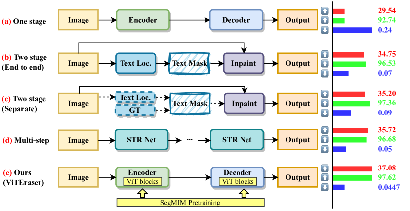
Figure 1: Comparison of ViTEraser with existing STR paradigms. Our method revisits the conventional single-step one-stage framework and improves it with ViTs for feature modeling and the proposed SegMIM pre-training. Without bells and whistles, ViTEraser achieves state-of-the-art performance on SCUT-EnsText [30]. The PSNR (red), MSSIM (green), and MSE (blue, %) metrics of representative methods [7],[21],[28],[18] of categories (a)-(d) are presented on the right. The full comparison can be found in Tab. IV. The dashed arrows indicate cutting off the gradient flow. (Loc. : Localize; GT: Ground Truth.)

Despite the great success achieved by previous methods, there are still two critical issues that remain to be solved. (1) The prominent two-stage methods achieve state-of-the-art performance but suffer from complex system design with two sub-models. The sequential text localizing and background inpainting pipeline introduces additional parameters, decreases the inference speed, and, more importantly, breaks the integrity of the entire model. The error of text localization can be easily propagated to the background inpainting, especially for the methods [23, 24, 25, 26, 27, 28, 29] that require pre-supplied text detectors [31, 32, 33]. (2) Recent advanced methods, regardless of one-stage-based [30, 8] or two-stage-based [13, 14, 18, 19, 21, 20], tend to devise a multi-step text erasing paradigm, e.g., coarse-to-fine or even progressive style, which undermines efficiency compared with single-step text erasing. Furthermore, it is difficult to properly balance each erasing step for these approaches. For instance, a lightweight refining network after a heavy coarse-erasing network [30] may cause remnants of text traces. Moreover, progressive approaches using identical weight-sharing networks [14] require the same network architecture and parameters to generalize to different degrees of text salience across multiple iterations.

To this end, we revisit the one-stage paradigm and propose a novel simple-yet-effective ViT-based method for STR, termed as ViTEraser. Fig. 1 compares our method with existing STR approaches. The ViTEraser follows the conventional one-stage framework [7] which comprises a single-step encoder-decoder network and is free of text mask input or text localizing sub-models, yielding a concise and elegant pipeline. This type of one-stage method perfectly gets rid of the drawbacks of the two-stage and multi-step approaches mentioned above, but has been discarded in recent advances because of the unexpected artifacts on non-text regions and inexhaustive erasure on text regions caused by the implicit integration of text localization and background inpainting into a single network. However, we argue that these limitations are actually due to the insufficient capacity of CNN-based architecture that is widely adopted in previous STR models. Recently, vision Transformers (ViT) [34, 35] have achieved incredible success on diverse computer vision tasks [36, 37, 38, 39, 40, 41]. However, the application of ViT to STR has rarely been investigated. Liu et al. [28] proposed local-global content modeling (LGCM) which utilizes Transformer to capture long-range dependency among pixels; however, the main structure of the network is still convolutional. Nevertheless, the ViT is perfect for STR since global information is indispensable for determining text locations and background textures, especially for large texts that existing STR systems still struggle with. Furthermore, plenty of studies [42, 43] have demonstrated that a multi-task Transformer surpasses a combination of sub-modules since the Transformer inherently encourages the interaction and complementarity of sub-tasks.

Therefore, for the first time in the STR field, the proposed ViTEraser thoroughly utilizes ViTs for feature representation in both the encoder and decoder. Specifically, the encoder hierarchically maps the input image into the hidden space through ViT blocks and patch embedding layers, while the decoder gradually upsamples the hidden features to the text-erased image with ViT blocks and patch splitting layers. Thanks to the high generality of the overall framework, different types of ViT blocks (e.g., Swin Transformer (v2) [44, 45], PVT [46, 47]) can be effortlessly integrated into ViTEraser, yielding a continuously developing STR method along with the progress of ViT.

Despite the powerful ViT-based structure, the implicit integration of text localizing and background inpainting still significantly challenges the model capacity of ViTEraser, requiring both high-level text perception and fine-grained pixel infilling abilities. However, the insufficient scale of existing STR datasets [30] limits the full learning of these abilities and makes the large-capacity ViT-based model prone to overfitting. To solve similar issues, pretraining plays a crucial role in a variety of fields including scene text recognition [48], document understanding [49, 50], and natural language processing [51], but is quite under-explored in the STR realm. Du et al. [18] pretrained the model by minimizing the discrepancy between generated text masks of differently augmented samples. However, since a pre-supplied stroke module has already provided the text location, such pretraining only enhances the background recovering abilities. With the rapid development of large-scale text detection datasets [52, 53, 54, 55, 56, 57, 58, 59, 60, 61, 62, 63] and commercial optical character recognition (OCR) APIs, numerous real-world images with text bounding boxes are easily available. Therefore, it is practical and meaningful to fully utilize existing large-scale text detection data for the pretraining of STR models. To this end, we propose a novel pretraining method for STR, termed SegMIM. Concretely, by assigning two pretraining tasks of text box segmentation and mask image modeling (MIM) [64, 65] to the output features of the encoder and decoder, respectively, the performance of text removal can be effectively enhanced. Furthermore, the high mask ratio (0.6) of MIM enables the model to learn the global relationship between both texts and backgrounds.

Extensive experiments are conducted on two popular STR benchmarks including SCUT-EnsText [30] and SCUT-Syn [7]. We comprehensively explore the architecture, pretraining, and scalability of the ViT-based encoder-decoder for STR. The experimental results demonstrate the effectiveness of ViTEraser with and without the SegMIM pretraining, outperforming previous methods by a significant margin. We also extend the ViTEraser to the tampered scene text detection (TSTD) task. The state-of-the-art performance on the Tampered-IC13 [66] dataset verifies the strong generality of ViTEraser.

In summary, the contributions of this paper are as follows.

1. We propose a novel ViT-based one-stage method for STR, termed as ViTEraser. The ViTEraser adopts a concise single-step encoder-decoder paradigm, effectively integrating ViTs for feature representation in both the encoder and decoder.

2. We propose SegMIM, a new pretraining scheme for STR. With SegMIM, ViTEraser acquires enhanced global reasoning capabilities, enabling it to effectively distinguish and generate text and background regions.

3. We conduct a comprehensive investigation into the architecture, pretraining, and scalability of the ViT-based encoder-decoder for STR, which provides deep insights into the application of the Transformer to this field.

4. The experiments demonstrate that ViTEraser achieves state-of-the-art performance on STR, and its potential for extension to other domains is also highlighted.

II Related Work

II-A Scene Text Removal

Scene text removal (STR) aims at realistically erasing the texts in natural scenes. Previous studies categorized existing STR approaches into one-stage and two-stage paradigms, following a simple criterion that the latter relies on external detectors while the former does not. Consequently, some methods, which contain text localizing sub-models to produce explicit text masks as subsequent inputs but end-to-end train these sub-models with other components, are classified into one-stage categories. However, these methods are not truly one-stage because their performance is still limited by the text localizing accuracy, which is also the most important drawback of the two-stage methods. Therefore, we re-identify this type of approach as the end-to-end two-stage method and traditional two-stage approaches as the separate two-stage method.

One-stage methods follow a concise image-to-image translation pipeline, implicitly integrating text localizing and background inpainting procedures into a single network. Nakamura et al. [2] pioneered in erasing texts at the image-patch level using a convolution-to-deconvolution encoder-decoder structure with skip connections. However, patch-level text erasing causes discontinuities during post-composition and can not handle large texts. Inspired by Pix2Pix [12], Zhang et al. [7] employed an end-to-end cGAN-based [10] network for image-level STR with a local-aware discriminator and a set of refined losses, yield significant improvement on STR quality. Liu et al. [30] improved EnsNet [7] with a two-step network, termed EraseNet, for coarse-to-refine text erasure. From a data perspective, Jiang et al. [8] proposed a controllable synthesis module based on EraseNet.

Two-stage methods decompose STR into text localizing and background inpainting sub-models. The text localizing sub-models produce explicit text masks which are fed into subsequent modules to facilitate text erasure. The two-stage methods can be further divided into separate and end-to-end categories. The separate two-stage methods depend on separately trained text detectors or ground truth (GT) to obtain text masks. Tursun et al. [24] proposed MTRNet that takes GT text masks as input for stable training and selective erasure. Similarly, Lee et al. [29] improved STR performance with GT text masks using gated attention and region-of-interest generation. Assuming text detection results have already been provided, there exist methods [23, 26] that directly performed text erasing on cropped text-line images. Differently, Liu et al. [28] adopted a PAN [33] for text detection and explored local-global clues for accurate background recovery. To eliminate the need for paired images, several studies [25, 27] separately trained localizing and inpainting models and then concatenated them. In contrast to separate two-stage methods, end-to-end two-stage methods end-to-end optimize the text localizing sub-models with other components. Keserwani et al. [16] sequentially performed text segmentation and text concealment. Following a coarse-to-refine paradigm, MTRNet++ [13] and SAEN [21] predicted coarse results and text stroke maps in parallel at the first stage and feed both predictions into the refinement stage. Inspired by progressive approaches [31], recent methods [14, 20, 19, 18] investigated multi-step text erasing with text segmentation modules. On the contrary, Hou et al. [17] expanded the width of the network in a multi-branch fashion. Operating at the feature level, FETNet [22] designed a feature erasing and transferring mechanism with the guidance of predicted text segmentation maps.

Our study re-explores the one-stage paradigm and demonstrates that such a simple framework that has nearly been discarded can achieve a clear state-of-the-art performance with proper ViT-based architecture and pretraining.

II-B Vision Transformer

The Transformer [34] was first proposed for natural language processing [51] but rapidly swept the computer vision field [36]. Limited by the $O(n^{2})$ computational complexity w.r.t. the sequence length, early ViTs [35, 67] first tokenized images with large window sizes and then kept the feature size throughout all the Transformer layers. Recently, the research on ViTs has focused on producing CNN-style [68, 69] hierarchical feature maps with various scales, such as PVT [46, 47], HVT [70], Swin Transformer [44, 45], and PiT [71], enabling fine granularity and dense predictions. Nowadays, ViTs have played an important role in many vision and cross-modal tasks, such as object detection [72], semantic segmentation [73], and document understanding [49, 50].

Despite the great success of ViTs, nearly all the existing STR approaches are CNN-based. In this paper, the proposed ViTEraser is the first STR method to thoroughly exploit ViTs for feature representation in both the encoder and decoder. Most importantly, we comprehensively explore the architecture, pretraining, and scalability of the ViT-based encoder-decoder for STR.

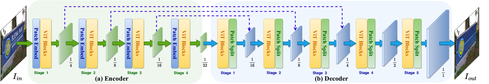
Figure 2: Overall architecture of ViTEraser. The ViTEraser follows the one-stage paradigm but is thoroughly equipped with ViTs for enhanced long-range context modeling, yielding a simple-yet-effective STR approach that is free of progressive refinements and text localizing sub-models. Specifically, (a) the encoder hierarchically maps the input image into the hidden space through ViT blocks and patch embedding layers, while (b) the decoder gradually upsamples the hidden features to the text-erased image with ViT blocks and patch splitting layers. The lateral connections (dashed arrows) shortcut the propagation of the image details from the encoder to the decoder. Furthermore, various ViTs can be easily inserted into ViTEraser, exhibiting high generality and flexibility.

III ViTEraser

III-A Overview

The overall framework of the proposed ViTEraser is shown in Fig. 2. ViTEraser revisits the conventional single-step one-stage paradigm, getting rid of the complicated iterative refinement and the susceptibility to text localizing accuracy. To compete with developed progressive and two-stage methods, the ViTEraser pioneers in thoroughly employing ViTs instead of CNN to extract features for STR in both the encoder and decoder, yielding a simple-yet-effective approach that significantly outperforms previous arts. Concretely, the encoder hierarchically maps the input image into the hidden space through successive ViT blocks and patch embedding layers, while the decoder gradually upsamples the hidden features to the text-erased image with successive ViT blocks and patch splitting layers. The ViT blocks throughout the encoder-decoder provide sufficient global context information, enabling the implicit integration of text localization and background inpainting into a single network within a single forward pass. Following previous approaches [2, 7, 30], lateral connections are devised between the encoder and decoder to preserve the details of the input image. Moreover, different types of ViTs can be effortlessly integrated into the ViTEraser, exhibiting high generality and flexibility.

During training, the ViTEraser is end-to-end optimized using a GAN-based scheme, incorporating a local-global discriminator [7, 30] and a set of refined losses (Sec. III-E).

III-B Encoder

As shown in Fig. 2(a), the encoder of ViTEraser consists of a sequence of four stages. Through these four stages, the encoder perceives an input image $I_{in}\in\mathbb{R}^{H\times W\times 3}$ with text strokes to remove and hierarchically produces four feature maps $\{f_{i}^{enc}\}_{i=1}^{4}$ with strides of $\{2^{i+1}\}_{i=1}^{4}$ w.r.t the input image and channels of $\{C_{i}^{enc}\}_{i=1}^{4}$, respectively. Specifically, the i-th stage first downsamples the spatial size using a patch embedding layer to reduce the subsequent computing cost and then globally captures the correlation between tokens through a stack of $N^{enc}_{i}$ ViT blocks (Sec. III-D).

III-B1 Patch Embedding Layer

A variety of studies [46, 44, 45, 47] have demonstrated the effectiveness of the patch embedding layer and its overlapping variants inserted into ViTs for spatial downsampling. Given an input feature map $f_{in}\in\mathbb{R}^{h\times w\times c_{in}}$, a patch embedding layer with a downsampling ratio of $d$ and an output channel of $c_{out}$ first flattens each $d\times d$ patch, yielding a $\frac{h}{d}\times\frac{w}{d}\times(d^{2}\times c_{in})$ feature map. Then a $1\times 1$ convolution layer is applied to transform this intermediate feature map into the output $f_{out}\in\mathbb{R}^{\frac{h}{d}\times\frac{w}{d}\times c_{out}}$. Note that the patch merging layer [44, 45] can be regarded as a special case of the patch embedding layer where the downsampling ratio is 2 and the out channel $c_{out}$ is equal to $2c_{in}$. As for the implementation of the encoder of ViTEraser, the input image is first tokenized using a $4\times 4$ window, i.e., the downsampling ratio of the 1st patch embedding layer is set to 4 while the others are 2, so as to suit the cutting-edge pyramid-like ViTs. Besides, the output channel of the i-th patch embedding layer is set to $C_{i}^{enc}$.

III-C Decoder

The pipeline of the decoder of ViTEraser is illustrated in Fig. 2(b), which is the concatenation of five stages. Taking the feature $f_{4}^{enc}\in\mathbb{R}^{\frac{H}{32}\times\frac{W}{32}\times C^{enc}_{4}}$ produced by the final stage of the encoder, the decoder hierarchically produces five feature maps $\{f_{i}^{dec}\in\mathbb{R}^{\frac{H}{2^{5-i}}\times\frac{W}{2^{5-i}}\times C_{i}^{dec}}\}_{i=1}^{5}$. Additionally, the features $\{f_{i}^{enc}\}_{i=1}^{3}$ of the encoder are laterally connected to the features $\{f_{4-i}^{dec}\}_{i=1}^{3}$ of the decoder, respectively, bringing detailed textures and contents of the input image. On top of the feature $f_{5}^{dec}\in\mathbb{R}^{H\times W\times C_{5}^{dec}}$ from the 5th stage, the text-erased image $I_{out}\in\mathbb{R}^{H\times W\times 3}$ is predicted through a $3\times 3$ convolution layer.

Concretely, in each stage of the decoder, the features are first processed with $N^{dec}_{i}$ ViT blocks (Sec. III-D) and then upsampled by 2 via a patch splitting layer. Empirically, the first four stages of the decoder are symmetric to the encoder, i.e., $\{N_{i}^{dec}\}_{i=1}^{4}$ and $\{C_{i}^{dec}\}_{i=1}^{3}$ is equal to $\{N_{5-i}^{enc}\}_{i=1}^{4}$ and $\{C_{4-i}^{enc}\}_{i=1}^{3}$, respectively.

III-C1 Patch Splitting Layer

To upsample the spatial size of feature maps, the patch splitting layer is designed as the inverse operation of the patched embedding layer described in Sec. III-B1. Fed with an input feature map $f_{in}\in\mathbb{R}^{h\times w\times c_{in}}$, the patch splitting layer first decomposes each $c_{in}$-dimensional token into a $2\times 2$ patch with $\frac{c_{in}}{4}$ dimension, expanding the input feature map to a shape of $2h\times 2w\times\frac{c_{in}}{4}$. After that, a $1\times 1$ convolution layer is adopted to transform the feature dimension, producing the output feature map $f_{out}\in\mathbb{R}^{2h\times 2w\times c_{out}}$ where $c_{out}$ of the i-th patch splitting layer is equal to $C_{i}^{dec}$.

III-C2 Lateral Connection

The architecture of lateral connections is inspired by EraseNet [30], which consists of non-linear, expanding, and shrinking transformations. For instance, if the feature $f_{1}\in\mathbb{R}^{h\times w\times c}$ is laterally connected to the feature $f_{2}$ of the same shape, the $f_{1}$ sequentially goes through one $1\times 1$ convolution with $c$ channels for non-linear transformation, two $3\times 3$ convolutions with $2c$ channels for expanding, and one convolution with $c$ channels for shrinking. Finally, the resulting feature is element-wise added to the feature $f_{2}$.

III-D ViT Blocks

The ViT block first models long-range dependencies using multi-head self-attention (MSA) and then applies a feed-forward network (FFN) to each position, finally producing an output feature map of the same shape as the input. Recent studies on ViTs mainly explore alleviating the high computational cost caused by the global self-attention on numerous tokens from the 2-dimensional image-like input. Although various ViT blocks can be effortlessly inserted into the framework of ViTEraser, in this paper, we focus on three types of ViT blocks, including (1) The block from Pyramid Vision Transformer [46] that replaces MSA with spatial-reduction attention (SRA), (2) Swin Transformer block [44] that utilizes shifted-window-based self-attention, and (3) Swin Transformer v2 block [45] that improves the performance on high-resolution inputs and training stability over the vanilla version.

III-E Training

During training, the ViTEraser is end-to-end optimized using a weighted sum of losses including text-aware multi-scale reconstruction loss, perceptual loss, style loss, segmentation loss, and adversarial loss.

Before introducing training details, we denote one training sample as $\{I_{in},I_{gt},M_{gt}\}$, where $I_{in}\in\mathbb{R}^{H\times W\times 3}$ is the input image with texts to remove, $I_{gt}\in\mathbb{R}^{H\times W\times 3}$ is the paired ground-truth (GT) image with all texts erased, and $M_{gt}\in\mathbb{R}^{H\times W\times 1}$ is the GT binary text mask at the bounding-box level (0 for backgrounds and 1 for text regions).

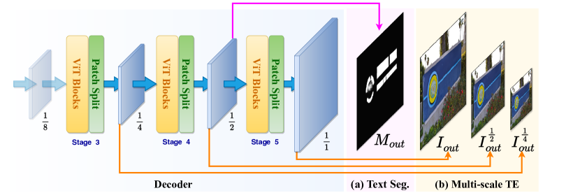
Figure 3: Auxiliary outputs of ViTEraser during training, including (a) text box segmentation map and (b) multi-scale text erasing results. (TE: text erasing)

III-E1 Auxiliary Output during Training

To effectively optimize the ViTEraser, auxiliary outputs are produced during only training, including a text box segmentation map $M_{out}$ and multi-scale text erasing results $\{I^{\frac{1}{2}}_{out},I^{\frac{1}{4}}_{out}\}$.

As depicted in Fig. 3(a), $M_{out}$ is predicted based on the feature map $f_{4}^{dec}\in\mathbb{R}^{\frac{H}{2}\times\frac{W}{2}\times C^{dec}_{4}}$ from the 4-th stage of the decoder. The $f_{4}^{dec}$ first goes through a $3\times 3$ deconvolution layer with spectral normalization [74] and a stride of 2, enlarging it to a shape of $H\times W\times 64$. Subsequently, the text box segmentation map $M_{out}\in\mathbb{R}^{H\times W\times 1}$ is produced via a $3\times 3$ convolution layer and a sigmoid activation. The value of $M_{out}$ is within the range of $(0,1)$, indicating the confidence that the corresponding pixel is located in text regions.

Except for the $I_{out}\in\mathbb{R}^{H\times W\times 3}$ (Sec. III-C), the multi-scale text erasing results $I^{\frac{1}{2}}_{out}\in\mathbb{R}^{\frac{H}{2}\times\frac{W}{2}\times 3}$ and $I^{\frac{1}{4}}_{out}\in\mathbb{R}^{\frac{H}{4}\times\frac{W}{4}\times 3}$ are predicted based on feature maps $f_{4}^{dec}\in\mathbb{R}^{\frac{H}{2}\times\frac{W}{2}\times C_{4}^{dec}}$ and $f_{3}^{dec}\in\mathbb{R}^{\frac{H}{4}\times\frac{W}{4}\times C_{3}^{dec}}$ from the 4th and 3rd stages of the decoder, respectively, each through a $3\times 3$ convolution layer.

III-E2 Text-Aware Multi-Scale Reconstruction Loss

The L1 loss is employed to measure the discrepancy between the predicted and GT text-erased images. To weigh the reconstruction of text and non-text regions, the GT text box masks are utilized to endow the loss with text-aware ability. Moreover, the reconstruction supervision is applied to the features at different levels of the decoder, so as to improve the multi-scale visual perception of the model. Denoting the multi-scale outputs $\{I_{out}^{\frac{1}{4}},I_{out}^{\frac{1}{2}},I_{out}\}$ as $\mathbb{I}_{out}$, the text-aware multi-scale reconstruction loss $\mathcal{L}_{msr}$ is formulated as

$$\mathcal{L}_{msr}= \sum\nolimits_{i=1}^{3}\lambda_{i}||(\mathbb{I}_{out(i)}-\mathbb{I}_{gt(i)})\odot\mathbb{M}_{gt(i)}||_{1}$$

$$+\beta_{i}||(\mathbb{I}_{out(i)}-\mathbb{I}_{gt(i)})\odot(1-\mathbb{M}_{gt(i)})||_{1},$$ (1)

where $\mathbb{I}_{gt(i)}$ and $\mathbb{M}_{gt(i)}$ denote the resized $I_{gt}$ and $M_{gt}$ corresponding to $\mathbb{I}_{out(i)}$, respectively. Besides, $\lambda$ and $\beta$ are empirically set to $\{5,6,10\}$ and $\{0.8,1,2\}$, respectively.

III-E3 Perceptual Loss

The perceptual loss [75] penalizes the differences between images from high-level perceptual and semantic perspectives. A VGG-16 [68] network $\Phi$ pretrained on ImageNet [76] is employed and $\Phi_{i}(x)$ represent the feature map of the i-th pooling layer with an input $x$. Mathematically, the perceptual loss $\mathcal{L}_{per}$ is calculated as

$$I_{out}^{*}= I_{out}\odot M_{gt}+I_{in}\odot(1-M_{gt}),$$ (2)

$$\mathcal{L}_{per}= \sum\nolimits_{i=1}^{3}||\Phi_{i}(I_{out})-\Phi_{i}(I_{gt})||_{1}$$

$$+\sum\nolimits_{i=1}^{3}||\Phi_{i}(I_{out}^{*})-\Phi_{i}(I_{gt})||_{1}\ .$$ (3)

III-E4 Style Loss

The style loss [77] constrains the style difference between images, which adopts a Gram matrix for high-level feature correlations. Using the same VGG-16-based $\Phi_{i}(\cdot)$ as the perceptual loss, the style loss $\mathcal{L}_{sty}$ is defined as

$$\mathcal{L}_{sty}= \sum\nolimits_{i=1}^{3}||Gram(\Phi_{i}(I_{out}))-Gram(\Phi_{i}(I_{gt}))||_{1}$$

$$+||Gram(\Phi_{i}(I_{out}^{*}))-Gram(\Phi_{i}(I_{gt}))||_{1},$$ (4)

where $I_{out}^{*}$ is computed as Eq. (2) and $Gram(\cdot)$ function calculates the Gram matrix of the given activation map.

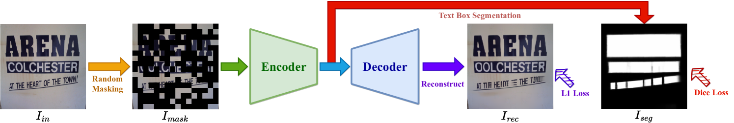
Figure 4: Pipeline of the proposed SegMIM pretraining. Given a randomly masked image, the text box segmentation and masked image modeling tasks are accomplished on top of the encoder and decoder, respectively. After end-to-end pretrained with large-scale scene text detection datasets, the network comprehensively learns the discriminative and generative features of texts and backgrounds, as well as a strong global reasoning capacity.

III-E5 Segmentation Loss

The ViTEraser end-to-end produces text-erased images from the scene text image inputs, without the guidance of any forms of text locations. However, the perception of text locations is critical to the text removal. Therefore, a segmentation loss $\mathcal{L}_{seg}$ is employed during training, with which the model learns to implicitly perceive text locations during inference. Specifically, $\mathcal{L}_{seg}$ is the dice loss between the predicted ($M_{out}$) and GT ($M_{gt}$) text box masks:

$$\mathcal{L}_{seg}=1-\frac{2\sum_{i,j}M_{out(i,j)}\times M_{gt(i,j)}}{\sum_{i,j}(M_{out(i,j)})^{2}+\sum_{i,j}(M_{gt(i,j)})^{2}}.$$ (5)

III-E6 Adversarial Loss

Adversarial training has been demonstrated effective for generating visually plausible content [7, 30, 28, 18, 22]. Inspired by EraseNet [30], a global-local discriminator $D$ is devised in our model training. The network $D$ takes a real/fake text-erased image and a binary mask as input and generates a value within $(-1,1)$ (1 for real, -1 for fake). To achieve this, the final feature map of $D$ is first activated with a sigmoid function, then rescaled to the range of $(-1,1)$, and finally averaged. Given the discriminator $D$, the adversarial losses can be defined as

$$\mathcal{L}_{adv}^{D}= max(0,1-D(I_{in},M_{gt}))$$

$$+max(0,1+D(I_{out},M_{gt})),$$ (6)

$$\mathcal{L}_{adv}^{G}= -D(I_{out},M_{gt}),$$ (7)

where $\mathcal{L}_{adv}^{D}$ and $\mathcal{L}_{adv}^{G}$ are used to optimize the discriminator $D$ and the generator (i.e., ViTEraser), respectively.

III-E7 Total Loss

The total loss $\mathcal{L}$ for ViTEraser is the weighted sum of the above losses, which is given by

$$\mathcal{L}=\alpha_{msr}\mathcal{L}_{msr}+\alpha_{per}\mathcal{L}_{per}+\alpha_{sty}\mathcal{L}_{sty}+\alpha_{seg}\mathcal{L}_{seg}+\alpha_{adv}\mathcal{L}_{adv}^{G},$$ (8)

where the weights $\alpha_{msr}$, $\alpha_{per}$, $\alpha_{sty}$, $\alpha_{seg}$, and $\alpha_{adv}$ are empirically set to 1, 0.01, 120, 1, and 0.1, respectively.

IV SegMIM Pre-Training

IV-A Motivation

As described above, the ViTEraser implicitly integrates the text localizing and background inpainting sub-tasks of STR into a single encoder-decoder without specific designs. Unlike two-stage methods that utilize task-specific modules and training objectives, the ViTEraser faces challenges in fully learning to handle both tasks and is susceptible to overfitting when scaled up. This limitation arises from the scarcity of training samples in STR and the high costs associated with annotating them. To this end, we leverage the availability of extensive scene text detection datasets. In doing so, we take advantage of large-scale pretraining techniques that have recently shown significant advancements in the fields of computer vision [48, 49, 50, 64, 65] and natural language processing [51]. Interestingly, the exploration of such pretraining methodologies has been rarely investigated in the previous literature on STR.

As the advancing of the scene text detection realm, there has emerged an increasing number of scene text detection datasets [52, 53, 54, 55, 56, 57, 58, 59], with scales ranging from early hundreds of samples [58] to recent tens of thousands [52]. Furthermore, developed OCR APIs provide a cost-free way of annotating text bounding boxes with high accuracy, which have already been widely applied to pretrain the Transformers for document understanding [49, 50]. Retrospectively, some STR approaches employed separately trained text detectors [25, 27, 28] or assumed that text locations have been pre-supplied [26, 24, 29, 19, 23], where the usage of large-scale text detection datasets has already been inevitable. Therefore, it is meaningful and practical to fully utilize existing large-scale scene text detection datasets for pretraining, which may be a promising direction that can accelerate the progress of STR.

IV-B Overview

Intuitively, the STR tasks can be decomposed into discriminative text localizing and generative background inpainting sub-processes. Furthermore, the model should first perceive the text locations and then fill them with proper backgrounds. Based on this straightforward idea, we propose a new pretraining paradigm for STR, termed SegMIM, which focuses the encoder on text box segmentation and the decoder on masked image modeling (MIM) during the end-to-end pretraining using existing large-scale scene text detection datasets, as shown in Fig. 4. Specifically, the image is first randomly masked in a SimMIM [65] manner before being fed to the network. Then, the text box segmentation and image reconstruction are performed based on the final features of the encoder and decoder, respectively.

Despite its simplicity, the clear advantages and interpretability of the proposed SegMIM are manifold. (1) The model learns the discriminative representation of texts and backgrounds through the text box segmentation task, which is crucial to STR. Retrospectively, Du et al. [18] pretrained the erasing network which includes a frozen pre-supplied stroke module for segmenting text strokes, overlooking the crucial ability to distinguish texts from backgrounds. (2) The model learns the generative features of both texts and backgrounds via masked image modeling. Specifically, the text reconstruction enhances the model perception of the shape and texture of texts, while the background recovery itself is crucial for STR. (3) The global reasoning capacity is significantly improved. With a high mask ratio (0.6), the model must induce the text locations and masked pixels through long-range dependencies, yielding a strong high-level semantic understanding of the scene image.

IV-C Architecture

The network architecture during pretraining inherits the encoder-decoder structure with lateral connections as Fig. 2 but with two extra heads for text box segmentation and image reconstruction, respectively. Given an input image $I_{in}\in\mathbb{R}^{H\times W\times 3}$, a binary mask $M_{mim}\in\mathbb{R}^{H\times W\times 1}$ is randomly generated following SimMIM [65] where 1 indicates masked pixels and 0 unmasked. Then, the masked image $I_{mask}$ combining $I_{in}$ and $M_{mim}$ is fed into the encoder-decoder.

IV-C1 Text Box Segmentation Head

The text box segmentation head corresponds to the red arrow in Fig. 4. Based on the final feature $f_{4}^{enc}\in\mathbb{R}^{\frac{H}{32}\times\frac{W}{32}\times C_{4}^{enc}}$ of the encoder, a $1\times 1$ convolution layer changes its dimension from $C_{4}^{enc}$ to $1024$. Subsequently, after transforming each $1024$-dimension vector to a $32\times 32$ patch and activating using a sigmoid function, a text box segmentation map $I_{seg}\in\mathbb{R}^{H\times W\times 1}$ is obtained.

IV-C2 Image Reconstruction Head

The purple arrow of Fig. 4 indicates the image reconstruction head. Through a $3\times 3$ convolution, a recovered image $I_{rec}\in\mathbb{R}^{H\times W\times 3}$ is predicted using the final feature $f_{5}^{dec}\in\mathbb{R}^{H\times W\times C_{5}^{dec}}$ of the decoder.

IV-D Optimization

The loss for pretraining $\mathcal{L}_{pre}$ is the sum of a text box segmentation loss $\mathcal{L}_{dice}$ and a masked image modeling loss $\mathcal{L}_{mim}$, which are calculated as

$$\mathcal{L}_{pre}= \mathcal{L}_{dice}+\mathcal{L}_{mim},$$ (9)

$$\mathcal{L}_{dice}= 1-\frac{2\sum_{i,j}I_{seg(i,j)}\times S_{gt(i,j)}}{\sum_{i,j}(I_{seg(i,j)})^{2}+\sum_{i,j}(S_{gt(i,j)})^{2}},$$ (10)

$$\mathcal{L}_{mim}= ||\Psi(I_{in},M_{mim})-\Psi(I_{rec},M_{mim})||_{1},$$ (11)

where $S_{gt}$ is the GT text box mask and the function $\Psi$ fetches the image pixels at masked positions.

V Experiments

V-A Datasets

V-A1 Scene Text Removal Datasets

The STR experiments are conducted on two widely used datasets, i.e., SCUT-EnsText [30] and SCUT-Syn [7].

SCUT-EnsText is a large-scale real-world STR dataset containing 2,749 samples for training and 813 samples for testing. The images are selected from diverse scene text benchmarks including ICDAR2013 [58], ICDAR2015 [57], COCO-Text [53], SVT [60], MLT2017 [54], MLT2019 [61], and ArT [59]. The paired text-erased images are carefully annotated by humans with high quality.

SCUT-Syn is a popular synthetic STR dataset. The training and testing sets contain 8,000 and 800 images, respectively. The samples are synthesized using the method proposed by Gupta et al. [78] with the background images from ICDAR2013 [58] and MLT2017 [54].

V-A2 Pretraining Datasets

The scene text detection datasets adopted for pretraining include the training sets of ICDAR2013 [58], ICDAR2015 [57], MLT2017 [54], ArT [59], LSVT [62], and ReCTS [63], as well as the training and validating sets of TextOCR [52]. Note that only fully annotated samples of LSVT are used. After removing the overlapping samples with the test set of SCUT-EnsText [30], there are a total of 98,340 valid samples for pretraining.

V-B Implementation Details

V-B1 Network Architecture

As described in Sec. III-D, we explore three types of ViT blocks, i.e., Pyramid Vision Transformer block (PVT), Swin Transformer block (Swin), and Swin Transformer v2 block (Swinv2), to implement the proposed ViTEraser. Moreover, using each type of ViT block, there are different scales of ViTEraser. Because the encoder adopts a general pipeline of hierarchical ViTs and the first four stages of the decoder are symmetric to the encoder, they can be easily configured following existing ViTs [44, 45, 46] of different scales. Thus, there remains only the last stage of the decoder which can be specified as follows:

• For the last stage of the decoder of PVT-based ViTEraser, the input dimension $C_{4}^{dec}$, output dimension $C_{5}^{dec}$, number of ViT blocks $N_{5}^{dec}$, number of heads of self-attention, the reduction ratio of SRA, and the expansion ratio of FFN are set to 32, 32, 2, 1, 16, and 8, respectively.

• For the last stage of the decoder of Swin(v2)-based ViTEraser, the input dimension $C_{4}^{dec}$, output dimension $C_{5}^{dec}$, number of ViT blocks $N_{5}^{dec}$, and number of heads of self-attention are set to $\frac{C_{3}^{dec}}{2}$, $\frac{C_{3}^{dec}}{4}$, 2, and 2, respectively.

In this way, we can easily obtain four flavors of PVT-based ViTEraser (ViTEraser-PVT-Tiny/Small/Medium/Large), three flavors of Swin-based ViTEraser (ViTEraser-Swin-Tiny/Small/Base), and three flavors of Swinv2-based ViTEraser (ViTEraser-Swinv2-Tiny/Small/Base).

V-B2 Pretraining

The SegMIM pretraining is conducted using the 98,340 samples specified in Sec. V-A2. The input image is resized to $512\times 512$. Following SimMIM [65], random masking is performed on the input image with a ratio of 0.6 and a patch size of 32. Besides, a mask token is added to the encoder to represent the masked patches. Using 4 NVIDIA A6000 GPUs with 48GB memory, the network is pretrained for 100 epochs with learning rates of 0.0001 before the 80th epoch and 0.00001 afterward, a batch size of 64, and an AdamW [79] optimizer. Because the mask token can negatively affect the encoder, the encoder will be finetuned solely with the text box segmentation task after end-to-end pretraining following the training strategy of SimMIM. Different from the pretraining, the finetuning lasts for 20 epochs with an initial learning rate of 0.00125 and a cosine decay learning rate schedule.

V-B3 Training

The training procedure on SCUT-EnsText or SCUT-Syn uses only its corresponding training set. If not specified, the pretrained weight with the classification task on ImageNet-1k [76] is used to initialize the encoder, while the decoder is randomly initialized. The input size of the images is set to $512\times 512$. The network is trained with an AdamW [79] optimizer for 300 epochs using 2 NVIDIA A6000 GPUs with 48GB memory. The learning rate is initialized as 0.0001 and linearly decayed to 0.00001 at the last epoch. The training batch size is set to 16.

V-C Evaluation Metrics

We perform a comprehensive evaluation of the text-erasing performance of ViTEraser using both the image-eval and detection-eval metrics. Specifically, following previous methods [7, 30, 28], the image-eval metrics include peak signal-to-noise ratio (PSNR), multi-scale structural similarity (MSSIM), mean square error (MSE), the average gray-level absolute difference (AGE), the percentage of error pixels (pEPs), the percentage of clustered error pixels (pCEPs), and Fréchet inception distance (FID). The detection-eval metrics involve precision (P), recall (R), and f-measure (F) following the ICDAR2015 [57] protocol, where the pretrained CRAFT [32] is selected as the text detector.

TABLE I: Comparison of different Transformer-based STR architectures. The MSSIM and MSE are presented in percent (%).

Encoder	Decoder	SCUT-EnsText							Params
		PSNR$\uparrow$	MSSIM $\uparrow$	MSE $\downarrow$	AGE$\downarrow$	pEPs$\downarrow$	pCEPs$\downarrow$	FID$\downarrow$
Conv.	DeConv.	35.05	97.20	0.0893	2.14	0.0111	0.0069	13.98	131.45M
Conv. + Trans. Enc.	DeConv.	34.85	97.13	0.1043	2.22	0.0120	0.0076	14.20	133.04M
Conv. + Trans. Enc.	Trans. Dec. + DeConv.	34.89	97.14	0.1007	2.20	0.0118	0.0074	14.12	139.43M
Swinv2-Tiny	DeConv.	36.06	97.40	0.0573	1.88	0.0079	0.0043	12.17	65.83M
Swinv2-Tiny	Trans. Dec. + DeConv.	35.92	97.39	0.0591	1.89	0.0082	0.0046	12.52	71.37M
Swinv2-Tiny	MLP	26.18	81.07	0.3532	7.32	0.0852	0.0157	38.90	28.21M
ViTEraser-Swinv2-Tiny		36.32	97.48	0.0569	1.81	0.0073	0.0040	11.77	65.39M

V-D Experiments on Architecture

Although the Transformer has revolutionized a wide variety of fields in recent years, its application to STR is quite under-explored. In this section, we try to answer the question that which architecture is the best for the integration of the Transformer into STR approaches. To this end, we compare the combinations of different encoders and decoders in Tab. I.

Encoder. (1) Conv. represents a ResNet50 [69]. (2) Conv. + Trans. Enc. indicates the concatenation of a ResNet50 and a Transformer encoder [34]. Following previous studies [42, 72], the Transformer encoder consists of 6 layers with 256 dimensions. (3) Swinv2-Tiny is the tiny version of Swin Transformer v2 [45]. Note that the ResNet50 and Swinv2-Tiny in the above encoders are pretrained with the classification task on ImageNet-1k.

Decoder. (1) DeConv. is a deconvolution-based decoder that is widely adopted in previous STR approaches. The DeConv. decoder hierarchically upsamples a feature map with a size of 16 and a dimension of 2048 to sizes of $\{32,64,128,256,512\}$ and dimensions of $\{1024,512,256,64,64\}$ through five deconvolution layers with spectral normalization [74], respectively. Based on the final feature map, the text-erased image is predicted using a $3\times 3$ convolution. Note that before being input to the DeConv. decoder, the feature map will first go through a $1\times 1$ convolution to transform the dimension to 2048. (2) Trans. Dec. + DeConv. adds a Transformer decoder before the DeConv. decoder to globally attend to the visual features extracted by the encoder. Similar to DETR [72], the Transformer decoder contains 6 layers with a dimension of 256. With 256 learnable queries, the Transformer decoder produces a hidden feature of 256 tokens and 256 channels which is subsequently resized to a shape of $16\times 16\times 256$ and then processed by the DeConv. decoder. (3) MLP follows the decoder of SegFormer [73]. The multi-scale features produced by the encoder are transformed to 256 dimensions, then interpolated to a size of $512\times 512$, and finally fused via a $1\times 1$ convolution. Based on the resulting feature map, the text erasing results are predicted using a $3\times 3$ convolution.

We combine different types of the above encoders and decoders and present their performances on SCUT-EnsText in Tab. I. Except for the architecture with MLP decoder, all models are trained in the same way as ViTEraser, with auxiliary outputs (Sec. III-E1) and multiple losses (Sec. III-E7). Since the MLP decoder does not generate multi-scale features, only one text-erased image can be predicted based on the final decoding feature. Therefore, the text-aware multi-scale reconstruction loss is degraded to a single-scale version.

Based on the results in Tab. I, we obtained the following observations and conclusions. (1) Simply inserting Transformer into fully convolutional networks can not obtain better STR results, comparing 2nd and 3rd rows with the 1st row. The reason may be that the Transformer encoder only performs global attention on the high-level features produced by CNN, omitting fine-grained correlations such as detailed textures. Moreover, the STR requires strict pixel-to-pixel spatial alignment; however, the Transformer decoder breaks such alignment but uses learnable queries to approximate the spatial matching between the input and output. (2) The architecture with pure ViT-based encoder (4th to 6th rows) makes significant progress on STR performance. The window-based Swinv2-Tiny can capture local and global dependencies at both low- and high-level feature spaces, yielding comprehensive and effective feature representations. It is worth noting that the combination of Swinv2-Tiny and DeConv. has already outperformed previous STR methods on SCUT-EnsText (Tab. IV). (3) The ViTEraser, which thoroughly utilizes ViTs for feature representation in both the encoder and decoder, provides the best architecture for applying the Transformer to STR with a substantial performance improvement over other architectures. The Swinv2 blocks at all depths of the decoder enable it to fill the background considering both surrounding pixels and long-distance context.

V-E Experiments on Pretraining

TABLE II: Comparison of different pretraining of ViTEraser-Swinv2-Small. The MSSIM and MSE are presented in percent (%).

Dataset	Encoder	Decoder	SCUT-EnsText
			PSNR$\uparrow$	MSSIM$\uparrow$	MSE$\downarrow$	AGE$\downarrow$	pEPs$\downarrow$	pCEPs$\downarrow$	FID$\downarrow$
×	×	×	33.34	96.70	0.1854	2.52	0.0161	0.0109	18.38
ImageNet-1k	Classification	×	36.55	97.56	0.0497	1.73	0.0072	0.0039	11.46
	SimMIM	×	36.38	97.51	0.0622	1.79	0.0076	0.0042	11.92
	Classification	Classification	36.54	97.55	0.0517	1.73	0.0073	0.0039	11.48
	Classification	SimMIM	36.45	97.55	0.0508	1.75	0.0082	0.0039	11.57
Scene Text Detection Dataset	Text Seg.	×	36.89	97.59	0.0490	1.73	0.0070	0.0038	10.98
	SimMIM	×	36.43	97.49	0.0554	1.77	0.0074	0.0040	11.82
	Text Seg.		36.78	97.57	0.0487	1.75	0.0070	0.0039	10.81
	SimMIM		36.68	97.58	0.0480	1.77	0.0067	0.0036	11.09
	SegMIM		37.08	97.62	0.0447	1.69	0.0064	0.0034	10.16

TABLE III: Comparison of different scales of ViTEraser-PVT/Swin/Swinv2. The MSSIM and MSE are presented in percent (%).

Architecture	Scale	SCUT-EnsText							Params
		PSNR$\uparrow$	MSSIM$\uparrow$	MSE$\downarrow$	AGE$\downarrow$	pEPs$\downarrow$	pCEPs$\downarrow$	FID$\downarrow$
ViTEraser-PVT	Tiny	34.48	96.98	0.1251	2.26	0.0124	0.0080	15.21	37.85M
	Small	35.03	97.15	0.1019	2.13	0.0112	0.0072	14.26	60.36M
	Medium	35.09	97.16	0.1089	2.12	0.0105	0.0066	13.95	99.80M
	Large	34.91	97.08	0.1183	2.17	0.0116	0.0074	14.48	134.13M
ViTEraser-Swin	Tiny	35.95	97.41	0.0647	1.87	0.0080	0.0045	12.38	65.26M
	Small	35.81	97.44	0.0589	2.01	0.0079	0.0044	11.94	107.90M
	Base	36.17	97.47	0.0637	1.80	0.0078	0.0044	12.11	191.66M
ViTEraser-Swinv2	Tiny	36.32	97.48	0.0569	1.81	0.0073	0.0040	11.77	65.39M
	Small	36.55	97.56	0.0497	1.73	0.0072	0.0039	11.46	108.15M
	Base	36.32	97.51	0.0565	1.86	0.0074	0.0041	11.68	191.97M

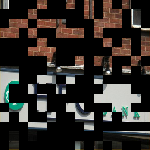
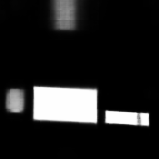
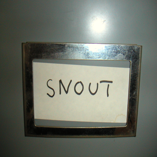
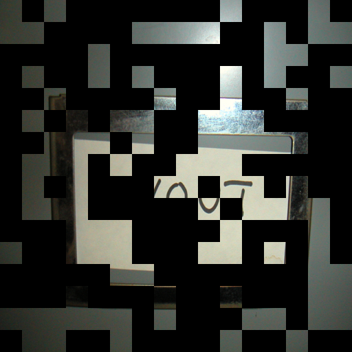
Figure 5: Visualization results of SegMIM-pretrained model. From left to right, the images are (a) original image, (b) masked image, (c) image reconstruction result, (d) predicted text box mask, and (e) GT text box mask. Zoom in for a better view.

It is known that pretraining is vital for Transformer-based approaches to exhibit superior performance. In this section, we comprehensively explore different pretraining schemes for the STR field based on ViTEraser. The experimental results based on ViTEraser-Swinv2-Small are listed in Tab. II.

The analyses of different pretraining strategies are as follows. (1) When the model is trained from scratch without any pretraining, the performance is quite unsatisfactory with only 33.34 dB PSNR and 96.70% MSSIM. (2) It is a common practice to exploit pretrained weights on ImageNet for plenty of computer vision tasks. We validate four ways of using the pretrained weights of Swinv2-Small with the classification or SimMIM [65] task on ImageNet-1k. When only the encoder is pretrained, the classification pretraining task is better than SimMIM. The reason may be that SimMIM focuses on pixel-level image reconstruction but lacks semantic-level learning that helps distinguish texts and backgrounds. Because the first four stages of the decoder are symmetric to the encoder, their parameters can also be initialized using the pretrained Swinv2-Small. However, no matter whether the classification or SimMIM weights are adopted for the decoder, the performance will slightly degrade, indicating that symmetrically transferring the pertrained weights for the encoder to the decoder can not preserve learned capacities. (3) The proposed SegMIM combines the text box segmentation and MIM tasks, yielding a significant improvement over the ImageNet-based pretraining. Moreover, the SegMIM also outperforms single text box segmentation or SimMIM pretraining of the encoder or encoder-decoder. The visualization results on the test set of ICDAR2013 (excluded from the pretraining dataset) of the SegMIM-pretrained model are shown in Fig. 5. Although 60% patches are masked, the model can infer complete text regions and fill the backgrounds and text regions with plausible contents, exhibiting strong global reasoning capacity.

V-F Experiments on Scalability

In Table III, we investigate the scalability of ViTEraser, where the performances of different scales of PVT-, Swin-, and Swinv2-based ViTEraser are presented. It can be seen that as the scale goes up, the performance tends to increase in general. However, for ViTEraser-Swinv2 and ViTEraser-PVT, the performance of the largest scale is inferior to a smaller one. This may be due to the overfitting caused by the dramatically increased parameters and limited training samples. More importantly, a large-scale Transformer-based network urgently requires proper pretraining to stimulate its potential (see Sec. V-G1 for further analyses).

Comparing different architectures, the ViTEraser-Swinv2 surpasses its counterparts with PVT or Swin block. Furthermore, the window-based Swin and Swinv2 blocks perform better than the PVT block. This may be due to that the PVT block increases the granularity as the feature resolution goes up, resulting in fewer details at two ends of the network. However, the ViTEraser-Swin/Swinv2 enjoys the window attention, simultaneously learning fine-grained details and global dependencies. Therefore, the Swinv2 block is employed in ViTEraser by default in the following experiments.

V-G Comparison with State of the Arts

TABLE IV: Comparison with state of the arts on SCUT-EnsText. The MSSIM, MSE, and Detection-Eval metrics are presented in percent (%). The $\dagger$ indicates SegMIM pretraining. The Swinv2 block is used in the ViTEraser. Bold denotes state of the art, while underline indicates the second best.

Method	Image-Eval							Detection-Eval$\downarrow$			Params$\downarrow$	Speed$\uparrow$ (fps)
	PSNR$\uparrow$	MSSIM$\uparrow$	MSE$\downarrow$	AGE$\downarrow$	pEPs$\downarrow$	pCEPs$\downarrow$	FID$\downarrow$	R	P	F
Original	-	-	-	-	-	-	-	69.5	79.4	74.1	-	-
Pix2pix [12]	26.70	88.56	0.37	6.09	0.0480	0.0227	46.88	35.4	69.7	47.0	54.42M	133
STE [2]	25.47	90.14	0.47	6.01	0.0533	0.0296	43.39	5.9	40.9	10.2	-	-
EnsNet [7]	29.54	92.74	0.24	4.16	0.0307	0.0136	32.71	32.8	68.7	44.4	12.40M	199
MTRNet++ [13]	29.63	93.71	0.28	3.51	0.0305	0.0168	35.68	15.1	63.8	24.4	18.67M	53
EraseNet [30]	32.30	95.42	0.15	3.02	0.0160	0.0090	19.27	4.6	53.2	8.5	17.82M	71
PERT [14]	33.25	96.95	0.14	2.18	0.0136	0.0088	-	2.9	52.7	5.4	14.00M	59
Tang et al. [26]	35.34	96.24	0.09	-	-	-	-	3.6	-	-	30.75M	7.8
PEN [18]	35.21	96.32	0.08	2.14	0.0097	0.0037	-	2.6	33.5	4.8	-	-
PEN* [18]	35.72	96.68	0.05	1.95	0.0071	0.0020	-	2.1	26.2	3.9	-	-
PSSTRNet [20]	34.65	96.75	0.14	1.72	0.0135	0.0074	-	5.1	47.7	9.3	4.88M	56
CTRNet [28]	35.20	97.36	0.09	2.20	0.0106	0.0068	13.99	1.4	38.4	2.7	159.81M	5.1
GaRNet$\S$ [29]	35.45	97.14	0.08	1.90	0.0105	0.0062	15.50	1.6	42.0	3.0	33.18M	22
MBE [17]	35.03	97.31	-	2.06	0.0128	0.0088	-	-	-	-	-	-
SAEN [21]	34.75	96.53	0.07	1.98	0.0125	0.0073	-	-	-	-	19.79M	62
FETNet [22]	34.53	97.01	0.13	1.75	0.0137	0.0080	-	5.8	51.3	10.5	8.53M	77
ViTEraser-Tiny	36.32	97.48	0.0569	1.81	0.0073	0.0040	11.77	0.717	32.7	1.403	65.39M	24
ViTEraser-Tiny$\dagger$	36.80	97.55	0.0491	1.79	0.0067	0.0036	10.79	0.430	27.3	0.847	65.39M	24
ViTEraser-Small	36.55	97.56	0.0497	1.73	0.0072	0.0039	11.46	0.778	42.2	1.528	108.15M	17
ViTEraser-Small$\dagger$	37.08	97.62	0.0447	1.69	0.0064	0.0034	10.16	0.430	30.9	0.848	108.15M	17
ViTEraser-Base	36.32	97.51	0.0565	1.86	0.0074	0.0041	11.68	0.635	37.8	1.248	191.97M	15
ViTEraser-Base$\dagger$	37.11	97.61	0.0474	1.70	0.0066	0.0035	10.15	0.389	29.7	0.768	191.97M	15

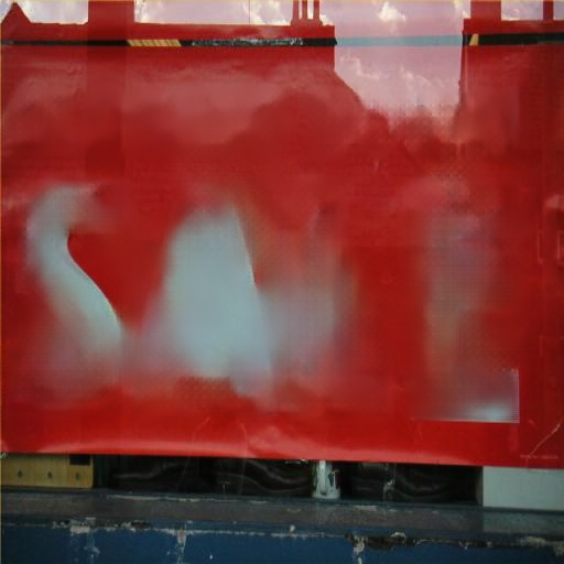
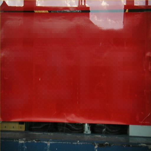
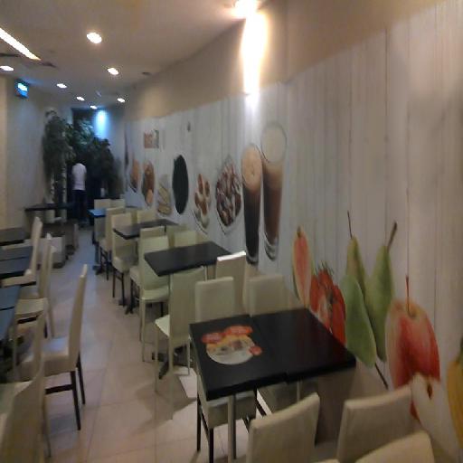
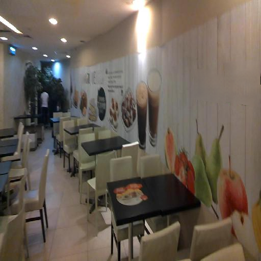
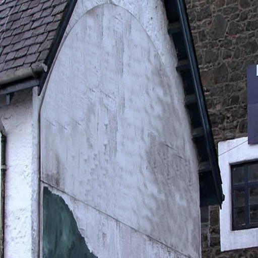
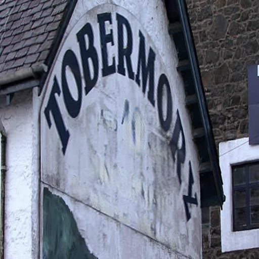
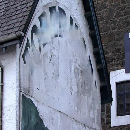
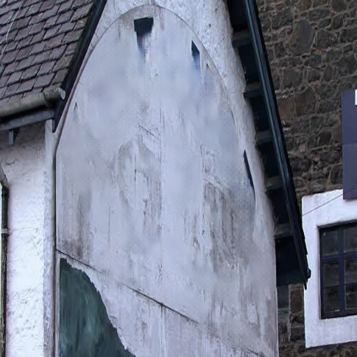
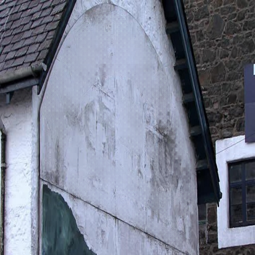
(a) Input

(b) GT

(c) MTRNet++

(d) EraseNet

(e) Tang et al.

(f) GaRNet

(g) CTRNet

(h) ViTEraser

Figure 6: Visualization results of existing methods and ViTEraser on SCUT-EnsText. From (c) to (g), the visualizations are from MTRNet++ [13], EraseNet [30], Tang et al. [26], GaRNet [29], and CTRNet [28]. The ViTEraser-Small (w/ SegMIM) is adopted in (h). Zoom in for a better view.

TABLE V: Comparison with state of the arts on SCUT-Syn. The MSSIM and MSE are presented in percent (%). The $\dagger$ indicates SegMIM pretraining. The Swinv2 block is used in the ViTEraser.

Method	PSNR$\uparrow$	MSSIM$\uparrow$	MSE$\downarrow$	AGE$\downarrow$	pEPs$\downarrow$	pCEPs$\downarrow$
Pix2pix [12]	26.76	91.08	0.27	5.47	0.0473	0.0244
STE [2]	25.40	90.12	0.65	9.49	0.0553	0.0347
EnsNet [7]	37.36	96.44	0.21	1.73	0.0069	0.0020
EraseNet [30]	38.32	97.67	0.02	1.60	0.0048	0.0004
MTRNet++ [13]	34.55	98.45	0.04	-	-	-
Zdenek et al. [25]	37.46	93.64	-	-	-	-
Conrad et al. [27]	32.97	94.90	-	-	-	-
PERT [14]	39.40	97.87	0.02	1.41	0.0045	0.0006
Tang et al. [26]	38.60	97.55	0.02	-	-	-
PEN [18]	39.26	98.03	0.02	1.29	0.0038	0.0004
PEN* [18]	38.87	97.83	0.03	1.38	0.0041	0.0004
PSSTRNet [20]	39.25	98.15	0.02	1.20	0.0043	0.0008
CTRNet [28]	41.28	98.52	0.02	1.33	0.0030	0.0007
MBE [17]	43.85	98.64	-	0.94	0.0013	0.00004
SEAN [21]	38.63	98.27	0.03	1.39	0.0043	0.0004
FETNet [22]	39.14	97.97	0.02	1.26	0.0046	0.0008
ViTEraser-Tiny	42.24	98.42	0.0112	1.23	0.0021	0.000020
ViTEraser-Tiny$\dagger$	42.40	98.44	0.0106	1.17	0.0018	0.000015
ViTEraser-Small	42.45	98.43	0.0109	1.19	0.0020	0.000019
ViTEraser-Small$\dagger$	42.66	98.49	0.0099	1.13	0.0016	0.000012
ViTEraser-Base	42.53	98.45	0.0102	1.19	0.0018	0.000016
ViTEraser-Base$\dagger$	42.97	98.55	0.0092	1.11	0.0015	0.000011

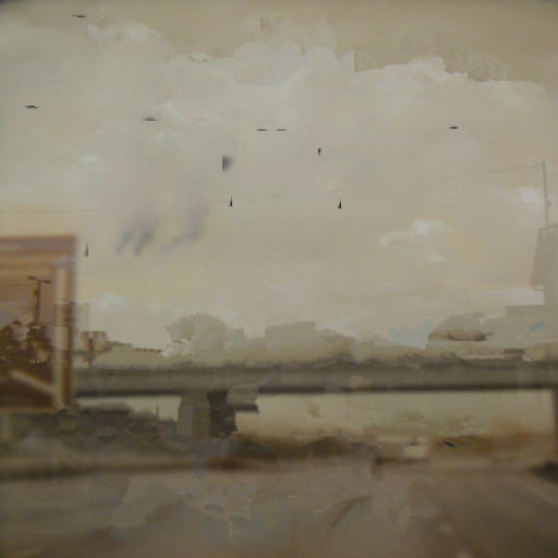
(a) Input

(b) GT

(c) EraseNet

(d) Tang et al.

(e) ViTEraser

Figure 7: Visualization results of previous methods and ViTEraser on SCUT-Syn. The text-erasing results are obtained by (c) EraseNet [30], (d) Tang et al. [26], and (e) ViTEraser-Base (w/ SegMIM). Zoom in for a better view.

V-G1 SCUT-EnsText

In Tab. IV, we comprehensively compare the ViTEraser of different scales with existing approaches on SCUT-EnsText. The image- and detection-eval metrics of Pix2Pix [12], STE [2], and EnsNet [7] are copied from [30] and [28]. The performance of MTRNet++ [13] is based on the reimplementation from GaRNet [29]. For a fair comparison, MTRNet++ uses empty coarse masks, and a pretrained CRAFT [32] is adopted to produce text box masks for GaRNet following Tang et al. [26] instead of using GT text box masks. All inference speeds are tested using an RTX3090 GPU, considering the time consumption of the model forward and post-processing. As for the model size, we calculate the number of minimum required parameters during inference, excluding auxiliary branches during training. Besides, the parameters and time cost of external text detectors are considered for Tang et al. [26], CTRNet [28], and GaRNet [29].

The quantitative results demonstrate the state-of-the-art performance of ViTEraser on real-world STR in terms of all the image-eval and detection-eval metrics. Specifically, in the aspect of image-eval metrics, a substantial improvement can be observed over previous methods, e.g., boosting PSNR from 35.72 dB to 37.11 dB. Notably, the recall and f-measure metrics of detection-eval reach a milestone of lower than 1%, indicating nearly all the texts have been effectively erased. Especially for ViTEraser-Base with SegMIM, remarkably low recall (0.389%) and f-measure (0.768%) have been achieved. Furthermore, compared with the other two scales, ViTEraser-Small is a better trade-off between performance, model size, and inference speed.

Moreover, SegMIM significantly boosts all three scales of ViTEraser, improving PSNRs of ViTEraser-Tiny, Small, and Base by 0.48, 0.53, and 0.79 dB, respectively. Owing to the overfitting caused by the substantially increased parameters, ViTEraser-Base without SegMIM is inferior to the Small counterpart. However, the SegMIM pretraining provides an effective initialization and fundamental STR-related knowledge, thus alleviating the overfitting problem. Consequently, the ViTEraser-Base can achieve better PSNR, FID, and detection-eval metrics compared with ViTErase-Small in the case of using SegMIM pretraining.

The visualization results of ViTEraser and representative previous approaches are shown in Fig. 6. Note that GT text masks are utilized in MTRNet++ [13], Tang et al. [26], GaRNet [29], and CTRNet [28]. Compared with existing methods, ViTEraser can effectively handle extremely large texts (1st row), tiny texts (2nd row), complex scenarios including arbitrarily curved and 3D texts (3rd to 5th rows), and fill in more realistic backgrounds (6th row), exhibiting strong robustness.

V-G2 SCUT-Syn

The quantitative comparison of ViTEraser and existing methods on the synthetic SCUT-Syn dataset is presented in Tab. V. It can be observed that ViTEraser can achieve state-of-the-art performance on SCUT-Syn except for the MBE [17] that ensembles multiple STR networks. Moreover, Fig. 7 shows the qualitative results on SCUT-Syn, demonstrating that ViTEraser can generate more visually plausible text-erased images without remnants of text traces.

TABLE VI: Comparison with existing methods on Tampered-IC13. The mF represents the average f-measure of real and tampered texts. All metrics are given in percent (%).

Method	Tampered Text			Real Text			mF
	R	P	F	R	P	F
S3R [66] + EAST	69.97	70.23	69.94	27.32	50.46	35.45	52.70
ViTEraser + EAST	77.87	79.66	78.76	32.45	65.23	43.34	61.05
S3R [66] + PSENet	79.43	79.92	79.67	41.89	61.56	49.85	64.76
ViTEraser + PSENet	82.38	83.23	82.80	39.70	64.96	49.28	66.04
S3R [66] + ContourNet	91.45	86.68	88.99	54.80	77.88	64.33	76.66
ViTEraser + ContourNet	92.62	85.77	89.06	56.84	75.82	64.97	77.02

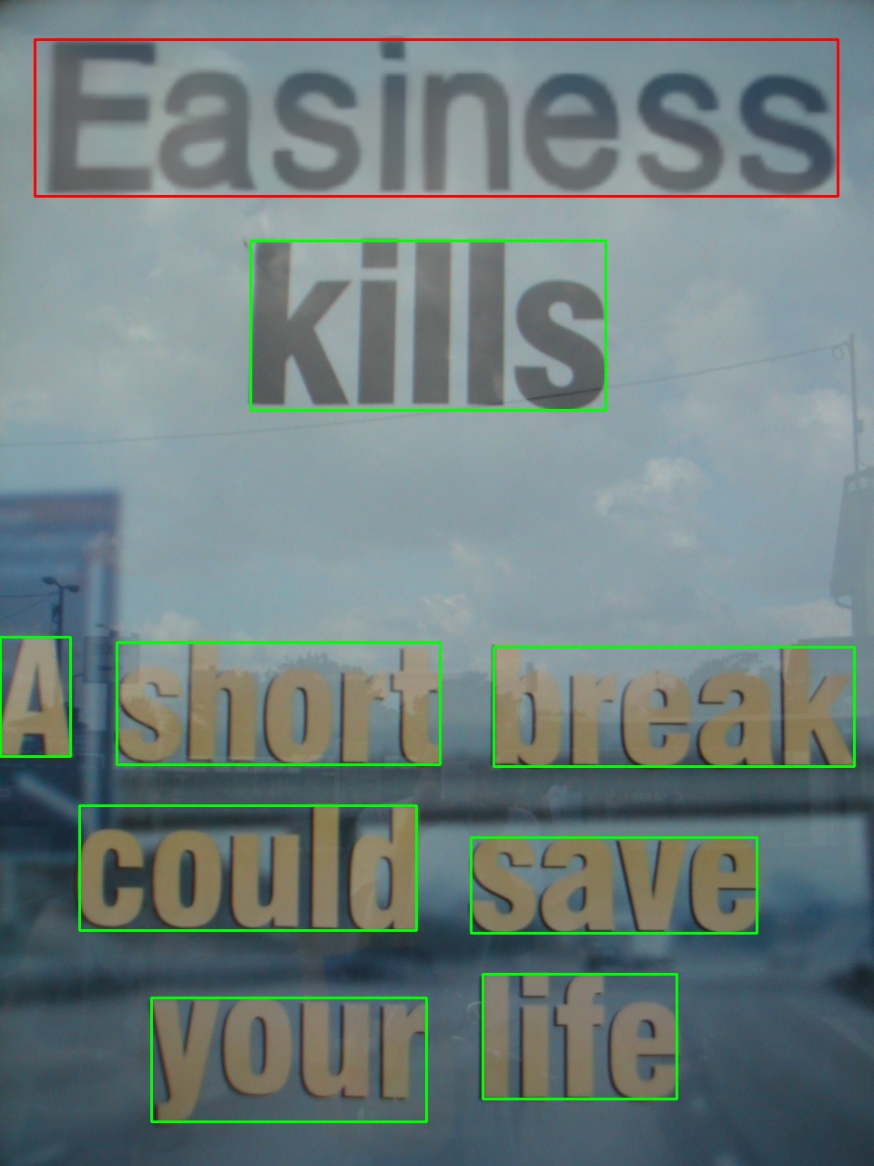
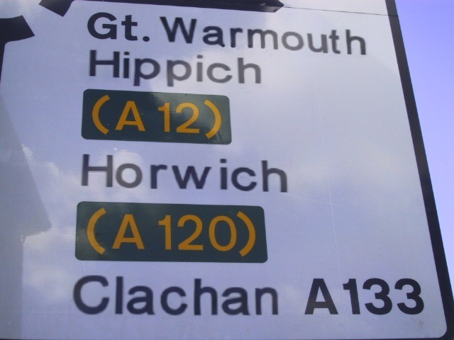
(a) Input

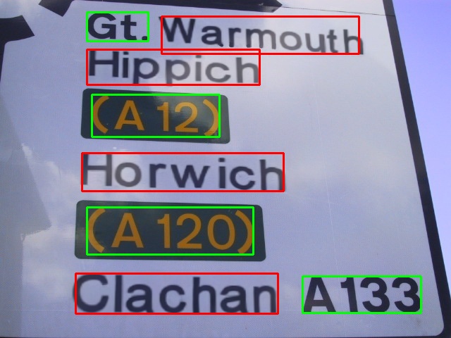
(b) GT

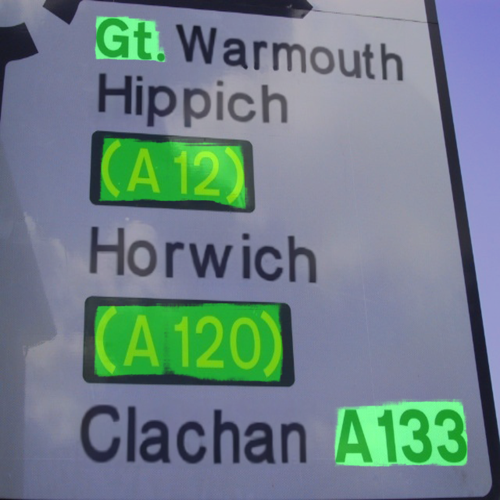
(c) Real

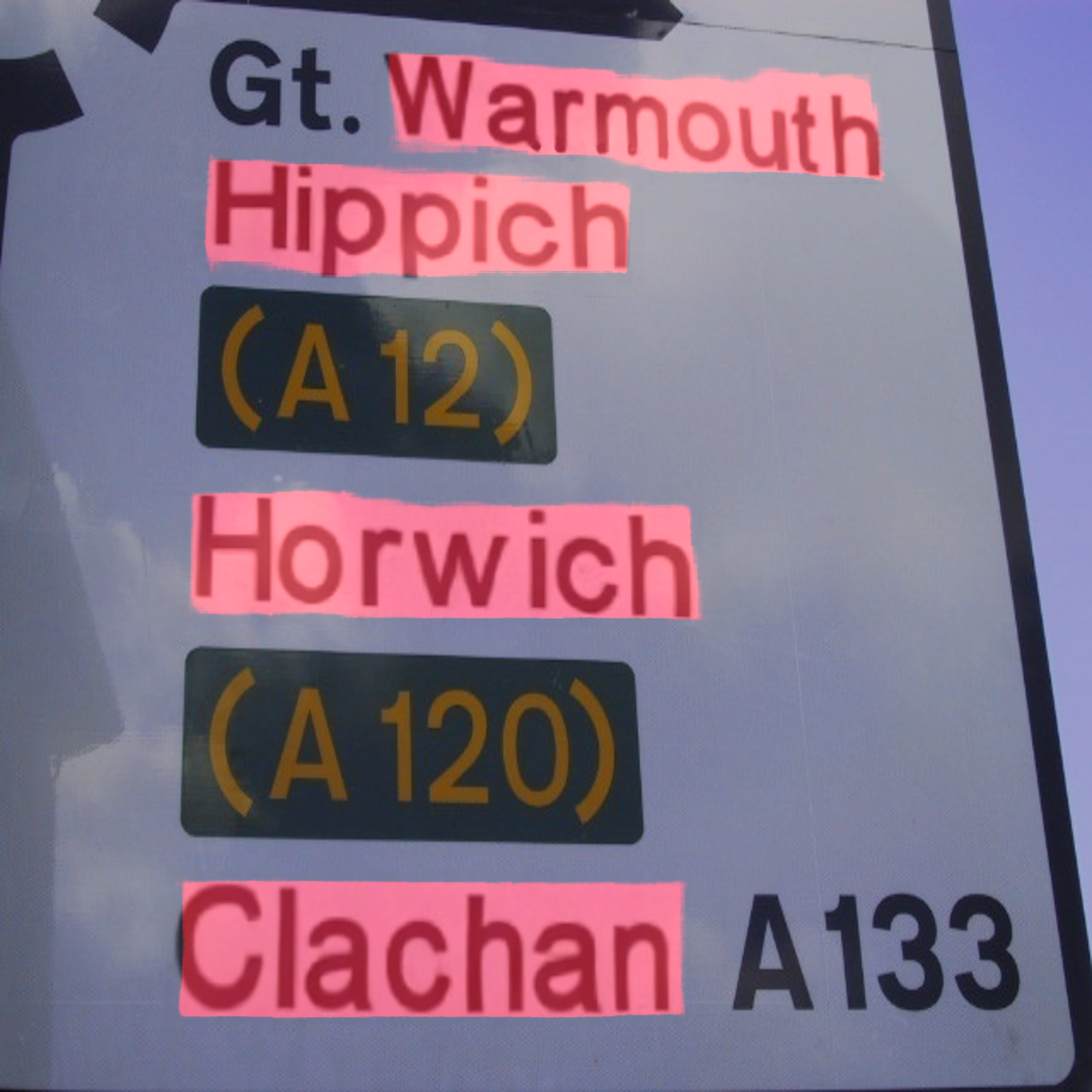
(d) Tampered

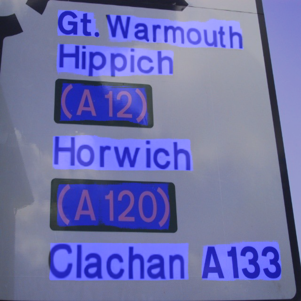
(e) Text

Figure 8: Visualization results on Tampered-IC13. From left to right, the images are the input, ground truth, real-text segmentation, tampered-text segmentation, and text segmentation, respectively. In the ground truth, the green and red boxes represent real and tampered texts, respectively.

V-H Extension

To verify the generalization ability of ViTEraser, we extend it to the tampered scene text detection (TSTD) task [66] that aims to localize both tampered and real texts from natural scenes. The experiments are conducted on the Tampered-IC13 dataset [66] which provides the bounding boxes of real and tampered texts. Using its training set, we train a ViTEraser-Tiny (w/o SegMIM) whose three-channel outputs correspond to the box-level segmentation of real texts, tampered texts, and both of them, respectively. The dice losses on these three segmentation maps are utilized to optimize the network. The visualization results of the test set are shown in Fig. 8, demonstrating ViTEraser can accurately localize tampered and real texts. Furthermore, to calculate the evaluation metrics [66] including recall (R), precision (P), and f-measure (F) of tampered and real texts, we incorporate an EAST [80], PSENet [31], or ContourNet [81] trained with Tampered-IC13 to produce bounding boxes of texts. Specifically, a bounding box will be regarded as tampered if more than 50% pixels within it are classified as tampered by ViTEraser. Similarly, the bounding boxes of real texts can also be determined. The quantitative performance is presented in Tab. VI. It can be seen that ViTEraser can achieve state-of-the-art performance on Tampered-IC13, showing strong generalization potential.

V-I Limitation

Despite the impressive performance achieved by the ViTEraser, its limitations lie in the large model size and relatively slow inference speed. As shown in Tab. IV, the ViTEraser-Tiny, Small, and Base contain 65M, 108M, and 192M parameters, as well as reach inference speeds of 24fps, 17fps, and 15fps, respectively. In comparison, most previous STR models, except for Pix2Pix [12] and CTRNet [28], keep their parameter sizes below 35M. Additionally, while the inference speed of ViTEraser may be adequate in real-world applications and is faster than several approaches including Tang et al. [26] and CTRNet [28], it is slower than many other methods. To address these limitations, future research aims to incorporate existing lightweight and efficient Transformer architectures to overcome the challenges associated with the large model size and slow inference speed in ViTEraser.

VI Conclusion

In this paper, we propose a novel simple-yet-effective one-stage ViT-based approach for STR, termed ViTEraser. ViTEraser employs a concise encoder-decoder paradigm, eliminating the need for explicit text localizing modules, external text detectors, and complex progressive refinement processes. For the first time in the STR field, ViTEraser thoroughly utilizes ViTs in place of CNNs for feature representation in both the encoder and decoder, significantly enhancing the long-range modeling ability. Furthermore, we propose a novel pretraining scheme, called SegMIM, which focuses the encoder and decoder on the text box segmentation and masked image modeling tasks, respectively. By leveraging existing large-scale text detection datasets, the SegMIM endows ViTEraser with discriminative and generative representations of texts and backgrounds as well as enhanced global reasoning capacity. Without bells and whistles, the proposed method substantially outperforms previous STR methods. Furthermore, we comprehensively explore the architecture, pretraining, and scalability of ViT-based encoder-decoder for STR, demonstrating the effectiveness of ViTEraser and SegMIM. It is worth mentioning that the ViTEraser can also demonstrate outstanding performance in tampered scene text detection, exhibiting strong generalization potential. We believe this study can inspire more research on ViT-based STR and contribute to the development of the unified model for pixel-level OCR tasks.

References

- [1] K. Inai, M. Pålsson, V. Frinken, Y. Feng, and S. Uchida, “Selective concealment of characters for privacy protection,” in Proc. Int. Conf. Pattern Recognit. (ICPR), 2014, pp. 333–338.
- [2] T. Nakamura, A. Zhu, K. Yanai, and S. Uchida, “Scene text eraser,” in Proc. Int. Conf. Doc. Anal. Recognit. (ICDAR), 2017, pp. 832–837.
- [3] L. Wu, C. Zhang, J. Liu, J. Han, J. Liu, E. Ding, and X. Bai, “Editing text in the wild,” in Proc. ACM Int. Conf. Multimed. (ACM MM), 2019, pp. 1500–1508.
- [4] Q. Yang, J. Huang, and W. Lin, “SwapText: Image based texts transfer in scenes,” in Proc. IEEE Conf. Comput. Vis. Pattern Recog. (CVPR), 2020, pp. 14 700–14 709.
- [5] P. Roy, S. Bhattacharya, S. Ghosh, and U. Pal, “STEFANN: Scene text editor using font adaptive neural network,” in Proc. IEEE Conf. Comput. Vis. Pattern Recog. (CVPR), 2020, pp. 13 228–13 237.
- [6] O. Tursun, S. Denman, S. Sivapalan, S. Sridharan, C. Fookes, and S. Mau, “Component-based attention for large-scale trademark retrieval,” IEEE Trans. Inf. Forensic Secur., vol. 17, pp. 2350–2363, 2019.
- [7] S. Zhang, Y. Liu, L. Jin, Y. Huang, and S. Lai, “EnsNet: Ensconce text in the wild,” in Proc. AAAI Conf. Artif. Intell. (AAAI), 2019, pp. 801–808.
- [8] G. Jiang, S. Wang, T. Ge, Y. Jiang, Y. Wei, and D. Lian, “Self-supervised text erasing with controllable image synthesis,” in Proc. ACM Int. Conf. Multimed. (ACM MM), 2022, pp. 1973–1983.
- [9] O. Ronneberger, P. Fischer, and T. Brox, “U-Net: Convolutional networks for biomedical image segmentation,” in Proc. Int. Conf. Med. Image Comput. Comput.-Assisted Intervention (MICCAI), 2015, pp. 234–241.
- [10] M. Mirza and S. Osindero, “Conditional generative adversarial nets,” arXiv preprint arXiv:1411.1784, 2014.
- [11] I. J. Goodfellow, J. Pouget-Abadie, M. Mirza, B. Xu, D. Warde-Farley, S. Ozair, A. Courville, and Y. Bengio, “Generative adversarial nets,” in Proc. Adv. Neural Inf. Process. Syst. (NeurIPS), 2014, pp. 2672–2680.
- [12] P. Isola, J.-Y. Zhu, T. Zhou, and A. A. Efros, “Image-to-image translation with conditional adversarial networks,” in Proc. IEEE Conf. Comput. Vis. Pattern Recog. (CVPR), 2017, pp. 1125–1134.
- [13] O. Tursun, S. Denman, R. Zeng, S. Sivapalan, S. Sridharan, and C. Fookes, “MTRNet++: One-stage mask-based scene text eraser,” Comput. Vis. Image Underst., vol. 201, p. 103066, 2020.
- [14] Y. Wang, H. Xie, S. Fang, Y. Qu, and Y. Zhang, “PERT: A progressively region-based network for scene text removal,” arXiv preprint arXiv:2106.13029, 2021.
- [15] J. Cho, S. Yun, D. Han, B. Heo, and J. Y. Choi, “Detecting and removing text in the wild,” IEEE Access, vol. 9, pp. 123 313–123 323, 2021.
- [16] P. Keserwani and P. P. Roy, “Text region conditional generative adversarial network for text concealment in the wild,” IEEE Trans. Circuits Syst. Video Technol., vol. 32, no. 5, pp. 3152–3163, 2021.
- [17] Y. Hou, J. J. Chen, and Z. Wang, “Multi-branch network with ensemble learning for text removal in the wild,” in Proc. Asian Conf. Comput. Vis. (ACCV), 2022, pp. 1333–1349.
- [18] X. Du, Z. Zhou, Y. Zheng, X. Wu, T. Ma, and C. Jin, “Progressive scene text erasing with self-supervision,” Comput. Vis. Image Underst., vol. 233, p. 103712, 2023.
- [19] X. Bian, C. Wang, W. Quan, J. Ye, X. Zhang, and D.-M. Yan, “Scene text removal via cascaded text stroke detection and erasing,” Comput. Vis. Media, vol. 8, pp. 273–287, 2022.
- [20] G. Lyu and A. Zhu, “PSSTRNet: Progressive segmentation-guided scene text removal network,” in Proc. IEEE Int. Conf. Multimedia Expo (ICME), 2022, pp. 1–6.
- [21] X. Du, Z. Zhou, Y. Zheng, T. Ma, X. Wu, and C. Jin, “Modeling stroke mask for end-to-end text erasing,” in Proc. IEEE Winter Conf. Appl. Comput. Vis. (WACV), 2023, pp. 6151–6159.
- [22] G. Lyu, K. Liu, A. Zhu, S. Uchida, and B. K. Iwana, “FETNet: Feature erasing and transferring network for scene text removal,” Pattern Recognit., p. 109531, 2023.
- [23] S. Qin, J. Wei, and R. Manduchi, “Automatic semantic content removal by learning to neglect,” in Proc. Br. Mach. Vis. Conf. (BMVC), 2018, pp. 1–12.
- [24] O. Tursun, R. Zeng, S. Denman, S. Sivapalan, S. Sridharan, and C. Fookes, “MTRNet: A generic scene text eraser,” in Proc. Int. Conf. Doc. Anal. Recognit. (ICDAR), 2019, pp. 39–44.
- [25] J. Zdenek and H. Nakayama, “Erasing scene text with weak supervision,” in Proc. IEEE Winter Conf. Appl. Comput. Vis. (WACV), 2020, pp. 2238–2246.
- [26] Z. Tang, T. Miyazaki, Y. Sugaya, and S. Omachi, “Stroke-based scene text erasing using synthetic data for training,” IEEE Trans. Image Process., vol. 30, pp. 9306–9320, 2021.
- [27] B. Conrad and P.-I. Chen, “Two-stage seamless text erasing on real-world scene images,” in Proc. Int. Conf. Image Process. (ICIP), 2021, pp. 1309–1313.
- [28] C. Liu, L. Jin, Y. Liu, C. Luo, B. Chen, F. Guo, and K. Ding, “Don’t forget me: Accurate background recovery for text removal via modeling local-global context,” in Proc. Eur. Conf. Comput. Vis. (ECCV), 2022, pp. 409–426.
- [29] H. Lee and C. Choi, “The surprisingly straightforward scene text removal method with gated attention and region of interest generation: A comprehensive prominent model analysis,” in Proc. Eur. Conf. Comput. Vis. (ECCV), 2022, pp. 457–472.
- [30] C. Liu, Y. Liu, L. Jin, S. Zhang, C. Luo, and Y. Wang, “EraseNet: End-to-end text removal in the wild,” IEEE Trans. Image Process., vol. 29, pp. 8760–8775, 2020.
- [31] W. Wang, E. Xie, X. Li, W. Hou, T. Lu, G. Yu, and S. Shao, “Shape robust text detection with progressive scale expansion network,” in Proc. IEEE Conf. Comput. Vis. Pattern Recog. (CVPR), 2019, pp. 9336–9345.
- [32] Y. Baek, B. Lee, D. Han, S. Yun, and H. Lee, “Character region awareness for text detection,” in Proc. IEEE Conf. Comput. Vis. Pattern Recog. (CVPR), 2019, pp. 9365–9374.
- [33] W. Wang, E. Xie, X. Song, Y. Zang, W. Wang, T. Lu, G. Yu, and C. Shen, “Efficient and accurate arbitrary-shaped text detection with pixel aggregation network,” in Proc. IEEE Int. Conf. Comput. Vis. (ICCV), 2019, pp. 8440–8449.
- [34] A. Vaswani, N. Shazeer, N. Parmar, J. Uszkoreit, L. Jones, A. N. Gomez, Ł. Kaiser, and I. Polosukhin, “Attention is all you need,” Proc. Adv. Neural Inf. Process. Syst. (NeurIPS), vol. 30, 2017.
- [35] A. Dosovitskiy, L. Beyer, A. Kolesnikov, D. Weissenborn, X. Zhai, T. Unterthiner, M. Dehghani, M. Minderer, G. Heigold, S. Gelly et al., “An image is worth 16x16 words: Transformers for image recognition at scale,” in Proc. Int. Conf. Learn. Represent. (ICLR), 2021, pp. 1–21.
- [36] K. Han, Y. Wang, H. Chen, X. Chen, J. Guo, Z. Liu, Y. Tang, A. Xiao, C. Xu, Y. Xu et al., “A survey on vision Transformer,” IEEE Trans. Pattern Anal. Mach. Intell., vol. 45, no. 1, pp. 87–110, 2022.
- [37] Y. Wang, H. Xie, S. Fang, M. Xing, J. Wang, S. Zhu, and Y. Zhang, “PETR: Rethinking the capability of Transformer-based language model in scene text recognition,” IEEE Trans. Image Process., vol. 31, pp. 5585–5598, 2022.
- [38] Y. Song, Z. He, H. Qian, and X. Du, “Vision Transformers for single image dehazing,” IEEE Trans. Image Process., vol. 32, pp. 1927–1941, 2023.
- [39] X. Liu, Q. Wang, Y. Hu, X. Tang, S. Zhang, S. Bai, and X. Bai, “End-to-end temporal action detection with Transformer,” IEEE Trans. Image Process., vol. 31, pp. 5427–5441, 2022.
- [40] Z. Xue, X. Tan, X. Yu, B. Liu, A. Yu, and P. Zhang, “Deep hierarchical vision Transformer for hyperspectral and lidar data classification,” IEEE Trans. Image Process., vol. 31, pp. 3095–3110, 2022.
- [41] T.-C. Hsu, Y.-S. Liao, and C.-R. Huang, “Video summarization with spatiotemporal vision Transformer,” IEEE Trans. Image Process., vol. 32, pp. 3013–3026, 2023.
- [42] D. Peng, X. Wang, Y. Liu, J. Zhang, M. Huang, S. Lai, J. Li, S. Zhu, D. Lin, C. Shen et al., “SPTS: Single-point text spotting,” in Proc. ACM Int. Conf. Multimed. (ACM MM), 2022, pp. 4272–4281.
- [43] P. Wang, A. Yang, R. Men, J. Lin, S. Bai, Z. Li, J. Ma, C. Zhou, J. Zhou, and H. Yang, “OFA: Unifying architectures, tasks, and modalities through a simple sequence-to-sequence learning framework,” in Proc. Int. Conf. Mach. Learn. (ICML), 2022, pp. 23 318–23 340.
- [44] Z. Liu, Y. Lin, Y. Cao, H. Hu, Y. Wei, Z. Zhang, S. Lin, and B. Guo, “Swin Transformer: Hierarchical vision Transformer using shifted windows,” in Proc. IEEE Int. Conf. Comput. Vis. (ICCV), 2021, pp. 10 012–10 022.
- [45] Z. Liu, H. Hu, Y. Lin, Z. Yao, Z. Xie, Y. Wei, J. Ning, Y. Cao, Z. Zhang, L. Dong et al., “Swin Transformer v2: Scaling up capacity and resolution,” in Proc. IEEE Conf. Comput. Vis. Pattern Recog. (CVPR), 2022, pp. 12 009–12 019.
- [46] W. Wang, E. Xie, X. Li, D.-P. Fan, K. Song, D. Liang, T. Lu, P. Luo, and L. Shao, “Pyramid vision Transformer: A versatile backbone for dense prediction without convolutions,” in Proc. IEEE Int. Conf. Comput. Vis. (ICCV), 2021, pp. 568–578.
- [47] Wang, Wenhai and Xie, Enze and Li, Xiang and Fan, Deng-Ping and Song, Kaitao and Liang, Ding and Lu, Tong and Luo, Ping and Shao, Ling, “PVT v2: Improved baselines with pyramid vision Transformer,” Comput. Vis. Media, vol. 8, no. 3, pp. 415–424, 2022.
- [48] M. Yang, M. Liao, P. Lu, J. Wang, S. Zhu, H. Luo, Q. Tian, and X. Bai, “Reading and writing: Discriminative and generative modeling for self-supervised text recognition,” in Proc. ACM Int. Conf. Multimed. (ACM MM), 2022, pp. 4214–4223.
- [49] Y. Xu, M. Li, L. Cui, S. Huang, F. Wei, and M. Zhou, “LayoutLM: Pre-training of text and layout for document image understanding,” in Proc. ACM SIGKDD Int. Conf. Knowl. Discov. Data Min. (KDD), 2020, pp. 1192–1200.
- [50] J. Wang, L. Jin, and K. Ding, “LiLT: A simple yet effective language-independent layout Transformer for structured document understanding,” in Proc. Annu. Meet. Assoc. Comput Linguist. (ACL), 2022, pp. 7747–7757.
- [51] J. D. M.-W. C. Kenton and L. K. Toutanova, “BERT: Pre-training of deep bidirectional Transformers for language understanding,” in Proc. Conf. N. Am. Chapter Assoc. Comput. Linguistics: Hum. Lang. Technol. (NAACL-HLT), 2019, pp. 4171–4186.
- [52] A. Singh, G. Pang, M. Toh, J. Huang, W. Galuba, and T. Hassner, “TextOCR: Towards large-scale end-to-end reasoning for arbitrary-shaped scene text,” in Proc. IEEE Conf. Comput. Vis. Pattern Recog. (CVPR), 2021, pp. 8802–8812.
- [53] A. Veit, T. Matera, L. Neumann, J. Matas, and S. Belongie, “COCO-Text: Dataset and benchmark for text detection and recognition in natural images,” arXiv preprint arXiv:1601.07140, 2016.
- [54] N. Nayef, F. Yin, I. Bizid, H. Choi, Y. Feng, D. Karatzas, Z. Luo, U. Pal, C. Rigaud, J. Chazalon et al., “ICDAR2017 robust reading challenge on multi-lingual scene text detection and script identification-RRC-MLT,” in Proc. Int. Conf. Doc. Anal. Recognit. (ICDAR), vol. 1, 2017, pp. 1454–1459.
- [55] Y. Liu, L. Jin, S. Zhang, C. Luo, and S. Zhang, “Curved scene text detection via transverse and longitudinal sequence connection,” Pattern Recognit., vol. 90, pp. 337–345, 2019.
- [56] C. K. Ch’ng and C. S. Chan, “Total-Text: A comprehensive dataset for scene text detection and recognition,” in Proc. Int. Conf. Doc. Anal. Recognit. (ICDAR), vol. 1, 2017, pp. 935–942.
- [57] D. Karatzas, L. Gomez-Bigorda, A. Nicolaou, S. Ghosh, A. Bagdanov, M. Iwamura, J. Matas, L. Neumann, V. R. Chandrasekhar, S. Lu et al., “ICDAR 2015 competition on robust reading,” in Proc. Int. Conf. Doc. Anal. Recognit. (ICDAR), 2015, pp. 1156–1160.
- [58] D. Karatzas, F. Shafait, S. Uchida, M. Iwamura, L. G. i Bigorda, S. R. Mestre, J. Mas, D. F. Mota, J. A. Almazan, and L. P. De Las Heras, “ICDAR 2013 robust reading competition,” in Proc. Int. Conf. Doc. Anal. Recognit. (ICDAR), 2013, pp. 1484–1493.
- [59] C. K. Chng, Y. Liu, Y. Sun, C. C. Ng, C. Luo, Z. Ni, C. Fang, S. Zhang, J. Han, E. Ding et al., “ICDAR2019 robust reading challenge on arbitrary-shaped text-RRC-ArT,” in Proc. Int. Conf. Doc. Anal. Recognit. (ICDAR), 2019, pp. 1571–1576.
- [60] K. Wang and S. Belongie, “Word spotting in the wild,” in Proc. Eur. Conf. Comput. Vis. (ECCV), 2010, pp. 591–604.
- [61] N. Nayef, Y. Patel, M. Busta, P. N. Chowdhury, D. Karatzas, W. Khlif, J. Matas, U. Pal, J.-C. Burie, C.-l. Liu et al., “ICDAR2019 robust reading challenge on multi-lingual scene text detection and recognition—RRC-MLT-2019,” in Proc. Int. Conf. Doc. Anal. Recognit. (ICDAR), 2019, pp. 1582–1587.
- [62] Y. Sun, Z. Ni, C.-K. Chng, Y. Liu, C. Luo, C. C. Ng, J. Han, E. Ding, J. Liu, D. Karatzas et al., “ICDAR 2019 competition on large-scale street view text with partial labeling-RRC-LSVT,” in Proc. Int. Conf. Doc. Anal. Recognit. (ICDAR), 2019, pp. 1557–1562.
- [63] R. Zhang, Y. Zhou, Q. Jiang, Q. Song, N. Li, K. Zhou, L. Wang, D. Wang, M. Liao, M. Yang et al., “ICDAR 2019 robust reading challenge on reading Chinese text on signboard,” in Proc. Int. Conf. Doc. Anal. Recognit. (ICDAR), 2019, pp. 1577–1581.
- [64] K. He, X. Chen, S. Xie, Y. Li, P. Dollár, and R. Girshick, “Masked autoencoders are scalable vision learners,” in Proc. IEEE Conf. Comput. Vis. Pattern Recog. (CVPR), 2022, pp. 16 000–16 009.
- [65] Z. Xie, Z. Zhang, Y. Cao, Y. Lin, J. Bao, Z. Yao, Q. Dai, and H. Hu, “SimMIM: A simple framework for masked image modeling,” in Proc. IEEE Conf. Comput. Vis. Pattern Recog. (CVPR), 2022, pp. 9653–9663.
- [66] Y. Wang, H. Xie, M. Xing, J. Wang, S. Zhu, and Y. Zhang, “Detecting tampered scene text in the wild,” in Proc. Eur. Conf. Comput. Vis. (ECCV), 2022, pp. 215–232.
- [67] H. Touvron, M. Cord, M. Douze, F. Massa, A. Sablayrolles, and H. Jégou, “Training data-efficient image transformers & distillation through attention,” in Proc. Int. Conf. Mach. Learn. (ICML), 2021, pp. 10 347–10 357.
- [68] K. Simonyan and A. Zisserman, “Very deep convolutional networks for large-scale image recognition,” in Proc. Int. Conf. Learn. Represent. (ICLR), 2015, pp. 1–14.
- [69] K. He, X. Zhang, S. Ren, and J. Sun, “Deep residual learning for image recognition,” in Proc. IEEE Conf. Comput. Vis. Pattern Recog. (CVPR), 2016, pp. 770–778.
- [70] Z. Pan, B. Zhuang, J. Liu, H. He, and J. Cai, “Scalable vision Transformers with hierarchical pooling,” in Proc. IEEE Int. Conf. Comput. Vis. (ICCV), 2021, pp. 377–386.
- [71] B. Heo, S. Yun, D. Han, S. Chun, J. Choe, and S. J. Oh, “Rethinking spatial dimensions of vision Transformers,” in Proc. IEEE Int. Conf. Comput. Vis. (ICCV), 2021, pp. 11 936–11 945.
- [72] N. Carion, F. Massa, G. Synnaeve, N. Usunier, A. Kirillov, and S. Zagoruyko, “End-to-end object detection with Transformers,” in Proc. Eur. Conf. Comput. Vis. (ECCV), 2020, pp. 213–229.
- [73] E. Xie, W. Wang, Z. Yu, A. Anandkumar, J. M. Alvarez, and P. Luo, “SegFormer: Simple and efficient design for semantic segmentation with Transformers,” in Proc. Adv. Neural Inf. Process. Syst. (NeurIPS), 2021, pp. 12 077–12 090.
- [74] T. Miyato, T. Kataoka, M. Koyama, and Y. Yoshida, “Spectral normalization for generative adversarial networks,” in Proc. Int. Conf. Learn. Represent. (ICLR), 2018, pp. 1–26.
- [75] J. Johnson, A. Alahi, and L. Fei-Fei, “Perceptual losses for real-time style transfer and super-resolution,” in Proc. Eur. Conf. Comput. Vis. (ECCV), 2016, pp. 694–711.
- [76] J. Deng, W. Dong, R. Socher, L.-J. Li, K. Li, and L. Fei-Fei, “ImageNet: A large-scale hierarchical image database,” in Proc. IEEE Conf. Comput. Vis. Pattern Recog. (CVPR), 2009, pp. 248–255.
- [77] L. A. Gatys, A. S. Ecker, and M. Bethge, “Image style transfer using convolutional neural networks,” in Proc. IEEE Conf. Comput. Vis. Pattern Recog. (CVPR), 2016, pp. 2414–2423.
- [78] A. Gupta, A. Vedaldi, and A. Zisserman, “Synthetic data for text localisation in natural images,” in Proc. IEEE Conf. Comput. Vis. Pattern Recog. (CVPR), 2016, pp. 2315–2324.
- [79] I. Loshchilov and F. Hutter, “Decoupled weight decay regularization,” in Proc. Int. Conf. Learn. Represent. (ICLR), 2019, pp. 1–18.
- [80] X. Zhou, C. Yao, H. Wen, Y. Wang, S. Zhou, W. He, and J. Liang, “EAST: An efficient and accurate scene text detector,” in Proc. IEEE Conf. Comput. Vis. Pattern Recog. (CVPR), 2017, pp. 5551–5560.
- [81] Y. Wang, H. Xie, Z.-J. Zha, M. Xing, Z. Fu, and Y. Zhang, “ContourNet: Taking a further step toward accurate arbitrary-shaped scene text detection,” in Proc. IEEE Conf. Comput. Vis. Pattern Recog. (CVPR), 2020, pp. 11 753–11 762.