HSR-Diff: Hyperspectral Image Super-Resolution via Conditional Diffusion Models

Abstract

Despite the proven significance of hyperspectral images (HSIs) in performing various computer vision tasks, its potential is adversely affected by the low-resolution (LR) property in the spatial domain, resulting from multiple physical factors. Inspired by recent advancements in deep generative models, we propose an HSI Super-resolution (SR) approach with Conditional Diffusion Models (HSR-Diff) that merges a high-resolution (HR) multispectral image (MSI) with the corresponding LR-HSI. HSR-Diff generates an HR-HSI via repeated refinement, in which the HR-HSI is initialized with pure Gaussian noise and iteratively refined. At each iteration, the noise is removed with a Conditional Denoising Transformer (CDFormer) that is trained on denoising at different noise levels, conditioned on the hierarchical feature maps of HR-MSI and LR-HSI. In addition, a progressive learning strategy is employed to exploit the global information of full-resolution images. Systematic experiments have been conducted on four public datasets, demonstrating that HSR-Diff outperforms state-of-the-art methods.

1 Introduction

Hyperspectral images (HSI) contain dozens or hundreds of spectral bands, enabling them to provide more faithful knowledge of targeted scenes than conventional imaging modalities. As such, HSIs play an irreplaceable role in various computer vision tasks, including classification [38, 43], segmentation [7], and tracking [36]. Although HSIs contain rich spectral information, contemporary hyperspectral imaging sensors lack high-resolution (HR) in the spatial domain, due to the stringent constraint of typically low signal-to-noise ratios. Their widespread use is significantly hindered by this fact. Restricted by hardware limitations, a practical way to work around this problem is to fuse the low-resolution (LR) HSI with an HR multispectral image (MSI). This requires the implementation of so-called HSI super-resolution (SR), as shown in Figure 1.

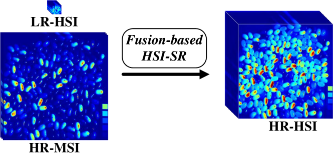
Figure 1: Illustration of HSI super-resolution.

Over the past few decades, a significant amount of research efforts have been devoted to developing HSI-SR approaches, which can be roughly classified into five categories [45]: Extensions of pansharpening [6], Bayesian inference-based [1, 34], matrix factorization-based [3], tensor-based [20], and deep learning (DL)-based. Whilst pansharpening methods [32] have been extended to the field of HSI-SR, such approaches are prone to spectral distortion. Bayesian inference-based approaches rely on the assumption of prior knowledge, thereby having a weak flexibility in dealing with different HSI structures. Matrix factorization-based techniques reshape the 3D HSIs and MSIs into matrices, thus facing the challenge of learning the required relationship between space and spectrum. Although several tensor-based methods have been proposed that can maintain the 3D structure of input images, they consume much more memory and computational power. Furthermore, these traditional approaches work via relying heavily on hand-crafted priors.

Recently, DL-based methods, especially convolutional neural network (CNN)-based approaches, have flooded over into the HSI-SR research community [8, 35, 11, 24, 47, 44, 21]. Rather than resorting to hand-crafted features, DL-based techniques learn prior knowledge automatically from given data. Particularly, Dong et al. proposed the first DL-based method for image SR, with the end-to-end mapping between LR images and HR images learned using a CNN [10]. Subsequently, generative adversarial networks (GANs) were introduced to the field of image SR in an effort to produce high-frequency details [19, 12]. After that, various GAN-based models have been devised, showing state-of-the-art results in the HSI-SR literature [29]. However, such work requires carefully designed regularization and optimization tricks to tame optimization instability and avoid mode collapse.

Inspired by the recent developments in deep generative models, in this paper, we propose an innovative approach that we refer to as HSR-Diff (HSI-SR with conditional diffusion models). It works by learning to transform the original standard normal distribution into the data distribution of HR-HSI through a sequence of refinements. In contrast to GAN-based methods which require inner-loop maximization, HSR-Diff minimizes a well-defined loss function. Although conditional diffusion models are straightforward to define and efficient to train, there has been no demonstration that they are capable of merging LR-HSI and HR-MSI to the best of our knowledge. We show that conditional diffusion models are capable of generating high-quality HR-HSIs, which may best the state-of-the-art results. A key factor of HSR-Diff is its inherent denoising ability thanks to use of deep neural networks. In spite of the effectiveness of CNNs for denoising, they have shown limitation in modelling long-range dependencies. To address the locality problem of convolution operations, a Conditional Denoising Transformer (CDFormer) is herein designed and trained with a denoising objective to remove various levels of noise iteratively. In addition, a progressive learning strategy is utilized to help the CDFormer learn the global statistics of full-resolution HSIs. The main contributions of this work are summarized as follows:

• We propose the novel application of conditional diffusion models in the field of HSI-SR that works by progressively destroying HR-HSI through injecting noise and subsequently learning to reverse this process, in order to perform HR-HSI.

• We introduce a CDFormer that refines a noisy HR-HSI conditioned on the deep feature maps of HR-MSI and LR-HSI, capable of modelling global connectivity with a self-attention mechanism.

• We employ a progressive learning strategy to exploit the global information of full-resolution HSIs, with CDFormer being trained on small image patches in the early epochs with high efficiency and on the global images in the later epochs to acquire global information.

• We present experimental investigations on four public datasets, with quantitative and qualitative results illustrating the superior performance of our approach as compared with state-of-the-art methods.

2 Related Work

2.1 Deep Generative Models

Typical deep generative models include autoregressive models (AR), normalizing flows (NF), variational autoencoders (VAE), GANs, and diffusion models. ARs learn data distribution via log-likelihood. Unfortunately, the low efficiency of sequential pixel generation limits their application to high-resolution images [31, 28]. NFs have the advantage of running at a high sampling speed, but their expressive ability is restricted by the need for invertible parameterized transformations with a tractable Jacobian determinant [25, 9, 17]. VAEs feature fast sampling while underperforming in comparison to GANs and ARs, in terms of image quality [18, 26, 30]. GANs are popular for class conditional image generation, and super-resolution [12]. However, the inner-outer loop optimization often requires tricks to stabilize training [2, 13], and conditional tasks like super-resolution usually demand an auxiliary consistency-based loss to avoid mode collapse [19].

The development of diffusion models has seen a dramatically accelerating pace over the past three years. Whilst diffusion models have shown great potential for a variety of computer vision applications, none of them have yet been devoted to the problem of HSI-SR to the best of our knowledge. In this paper, we extend the utility of diffusion models to the field of HSI-SR.

2.2 Deep Learning-Based HSI-SR

In recent years, data-driven CNN architectures have been shown to outperform traditional approaches for use in the HSI-SR literature. These methods formulate the underlying fusion problem as a highly nonlinear mapping that takes HR-MSIs and LR-HSIs as input to generate an optimal HR-HSI. For example, CMHF-net [35] is an interpretable CNN, the design of which exploits the deep unfolding technique. Zhang et al. [44] proposed to reconstruct HR-HSIs with a two-stage network, while Zhang et al. [46] designed an interpretable spatial-spectral reconstruction network (SSR-NET) based on CNN. Aiming at problems of inflexible structure and information distortion, Jin et al. embedded Bilateral Activation Mechanism into ResNet, resulting in the effective model of BRResNet [16]. Thanks to the inductive bias of CNN, such as locality and weight sharing, these methods can provide good generalization performance and achieve impressive results.

Nevertheless, CNNs have limitations in capturing long-range dependencies and self-similarity priors. To overcome such shortcomings we employ Transformer to learn global statistics of full-resolution images in this work.

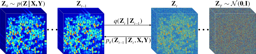
Figure 2: Forward and reverse processes of HSR-Diff, with forward process $q$ generating an HSI sequence (left to right) by gradually adding Gaussian noise, and reverse process $p$ iteratively refining HR-HSI (right to left).

3 Proposed Methodology

3.1 Problem Formulation

Without losing generality, the observation models for the HR-MSI and LR-HSI of interest can be mathematically formulated as

$$\mathbf{X}=\mathbf{R}\mathbf{Z},\mathbf{Y}=\mathbf{Z}\mathbf{D},$$ (1)

where $\mathbf{X}\in\mathbb{R}^{b\times HW}$ denotes the HR-MSI which consists of $b$ spectral bands with a spatial resolution of $HW$ in the spatial domain; $\mathbf{R}\in\mathbb{R}^{b\times B}$ represents the spectral response function of HR-MSI; $\mathbf{Y}\in\mathbb{R}^{B\times hw}$ denotes the LR-HSI; and $\mathbf{Z}\in\mathbb{R}^{B\times HW}$ is the latent HR-HSI. In the above, $b$ and $B$ are the numbers of bands, with $h$ and $H$ being the band height, and $w$ and $W$ the width, where $b\ll B$, $h\ll H$, and $w\ll W$. $\mathbf{D}\in\mathbb{R}^{HW\times hw}$ is the spatial response of the LR-HSI, which can be modelled with blurring and down-sampling operations. The HSI-SR can be interpreted as an inverse problem for merging a practically collected $\mathbf{X}$ and an observed $\mathbf{Y}$ to produce a latent $\mathbf{Z}$. In ths paper, the ideal $\mathbf{Z}$ is restored with HSR-Diff conditioned on spatio-spectral information of $\mathbf{X}$ and $\mathbf{Y}$, the details of which are described below.

3.2 HSI-SR with Conditional Diffusion Models

Given a dataset $\mathcal{D}_{train}=\{\mathbf{X}^{i},\mathbf{Y}^{i},\mathbf{Z}^{i}\}_{i=1}^{N}$ satisfying a certain joint probability distribution $p\left(\mathbf{X},\mathbf{Y},\mathbf{Z}\right)$, many pairs of $\left(\mathbf{X},\mathbf{Y}\right)$ may be consistent with the same $\mathbf{Z}$. Thus, the HR-HSI $\mathbf{Z}$ can be obtained with iterative refinements that provide an approximate to $p\left(\mathbf{Z}|\mathbf{X},\mathbf{Y}\right)$. In this work, we implement the process of iterative refinements with HSR-Diff, where the optimized HR-HSI is presumed to be produced in $T$ refinement steps. In HSR-Diff, the target HR-HSI is initialized with a pure noise $\mathbf{Z}_{T}\sim\mathcal{N}(\mathbf{0},\mathbf{I})$ as shown in Figure 2. The HSI is then refined iteratively according to learned conditional distributions $p_{\theta}\left(\mathbf{Z}_{t-1}|\mathbf{Z}_{t},\mathbf{X},\mathbf{Y}\right)$. In so doing, the image sequence $(\mathbf{Z}_{T-1},\mathbf{Z}_{T-2},\ldots,\mathbf{Z}_{0})$ can be attained and ultimately $\mathbf{Z}_{0}\sim p\left(\mathbf{Z}|\mathbf{X},\mathbf{Y}\right)$.

The HSR-Diff employed makes use of two processes: a forward process that perturbs HSI to noise, and a reverse process converting noise back to HSI. In the forward process, the intermediate images, i.e., $\mathbf{Z}_{T-1}$, $\mathbf{Z}_{T-2}$, $\cdots$, and $\mathbf{Z}_{1}$, are generated according to a Markov chain with fixed transition probability $q\left(\mathbf{Z}_{t}|\mathbf{Z}_{t-1}\right)$. We are interested in reversing the process via iterative refinements, in which the noise is reduced iteratively with a reverse Markov chain conditioned on $\mathbf{X}$ and $\mathbf{Y}$. The reverse chain is learned with the CDFormer $f_{\theta}$. Further details of HSR-Diff’s working are given below.

3.2.1 Forward Process

Inspired by [15], forward process $q$ iteratively adds Gaussian noise to $\mathbf{Z}_{0}$ over $T$ iterations:

$$q\left(\mathbf{Z}_{1:T}\mid\mathbf{Z}_{0}\right) =\prod_{t=1}^{T}q\left(\mathbf{Z}_{t}\mid\mathbf{Z}_{t-1}\right),$$ (2)

$$q\left(\mathbf{Z}_{t}\mid\mathbf{Z}_{t-1}\right) =\mathcal{N}\left(\mathbf{Z}_{t};\sqrt{\alpha_{t}}\mathbf{Z}_{t-1},\left(1-\alpha_{t}\right)\mathbf{I}\right),$$

where $\alpha_{1:T}\in(0,1)$ are scalar hyper-parameters. Note that in the forward process, the distribution of $\mathbf{Z}_{t}$ given $\mathbf{Z}_{0}$ can be directly sampled in closed form. This implies that

$$q\left(\mathbf{Z}_{t}\mid\mathbf{Z}_{0}\right)=\mathcal{N}\left(\mathbf{Z}_{t};\sqrt{\gamma_{t}}\mathbf{Z}_{0},\left(1-\gamma_{t}\right)\mathbf{I}\right)$$ (3)

where $\gamma=\prod_{i=1}^{t}\alpha_{i}$. In addition, the posterior distribution of $\mathbf{Z}_{t-1}$ given $\mathbf{Z}_{0}$ and $\mathbf{Z}_{t}$ can be derived by

$$q\left(\mathbf{Z}_{t-1}\mid\mathbf{Z}_{0},\mathbf{Z}_{t}\right)=\mathcal{N}\left(\mathbf{Z}_{t-1};\boldsymbol{\mu},\sigma^{2}\mathbf{I}\right)$$ (4)

$$\boldsymbol{\mu}=\frac{\sqrt{\gamma_{t-1}}\left(1-\alpha_{t}\right)}{1-\gamma_{t}}\mathbf{Z}_{0}+\frac{\sqrt{\alpha_{t}}\left(1-\gamma_{t-1}\right)}{1-\gamma_{t}}\mathbf{Z}_{t}$$

$$\sigma^{2}=\frac{\left(1-\gamma_{t-1}\right)\left(1-\alpha_{t}\right)}{1-\gamma_{t}}.$$

This posterior is useful in the reverse process.

3.2.2 Reverse Markovian Process

The reverse process inferences $\mathbf{Z}_{0}$ via iterative refinements. It starts from a pure Gaussian noise $\mathbf{Z}_{T}$ and goes in the opposite direction of the forward process:

$$p_{\theta}\left(\mathbf{Z}_{0:T}\mid\mathbf{X},\mathbf{Y}\right) =p\left(\mathbf{Z}_{T}\right)\prod_{t=1}^{T}p_{\theta}\left(\mathbf{Z}_{t-1}\mid\mathbf{Z}_{t},\mathbf{X},\mathbf{Y}\right)$$ (5)

$$p\left(\mathbf{Z}_{T}\right) =\mathcal{N}\left(\mathbf{Z}_{T};\mathbf{0},\mathbf{I}\right)$$

$$p_{\theta}\left(\mathbf{Z}_{t-1}\mid\mathbf{Z}_{t},\mathbf{X},\mathbf{Y}\right) =\mathcal{N}\left(\mathbf{Z}_{t-1};\mu_{\theta}\left(\mathbf{X},\mathbf{Y},\mathbf{Z}_{t},\gamma_{t}\right),\sigma_{t}^{2}\mathbf{I}\right),$$

where the distribution $p_{\theta}\left(\mathbf{Z}_{t-1}\mid\mathbf{Z}_{t},\mathbf{X},\mathbf{Y}\right)$ is parameterized with $\theta$. Note that the CDFormer provides a prediction of $\hat{\mathbf{Z}}_{0}$. Thus, according to (4), each refinement step takes the following form:

$$\mathbf{Z}_{t-1}= \frac{\sqrt{\gamma_{t-1}}\left(1-\alpha_{t}\right)}{1-\gamma_{t}}f_{\theta}\left(\mathbf{X},\mathbf{Y},\mathbf{Z}_{t},\gamma_{t}\right)$$ (6)

$$+\frac{\sqrt{\alpha_{t}}\left(1-\gamma_{t-1}\right)}{1-\gamma_{t}}\mathbf{Z}_{t}+\sqrt{1-\alpha_{t}}\boldsymbol{\epsilon},$$

where $\boldsymbol{\epsilon}\sim\mathcal{N}\left(\mathbf{0},\mathbf{I}\right)$ and $f_{\theta}$ is the CDFormer.

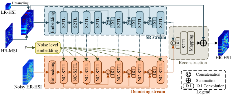
Figure 3: Architecture of Conditional Denoising Transformer.

3.2.3 Noise Schedule

Inspired by the research reported in [5], we sample $\gamma$ with two steps during training. In particular, we first sample a time step $t\sim U\left\{1,T\right\}$ and then randomly select $\gamma\sim U\left(\gamma_{t-1},\gamma_{t}\right)$. As such, $\gamma\sim p\left(\gamma\right)=\sum_{t=1}^{T}\frac{1}{T}U\left(\gamma_{t-1},\gamma_{t}\right)$. Normally, the model with a large $T$ can achieve better results. However, we find (through empirical investigations) that the performance is not very sensitive to the exact values of $T$. Therefore, no hyper-parameter search about $T$ is conducted and we set $T=2000$ for simplicity. As for the inference process, we set the maximum generation iterations to 100, employing a linear noise schedule.

3.3 Conditional Denoising Transformer

The property of non-local self-similarity of HSIs is often exploited in denoising tasks but is usually not well captured by CNN-based models. Due to the effectiveness of Transformer layer in capturing non-local long-range dependencies, the potential of Transformer is explored in conditional denoising of HSI. Unfortunately, the vanilla Transformer focuses only on spatial relationships between pixels while neglecting the spectral dimension. Besides, denoising networks in conditional diffusion models normally concatenate all images together as input, which may hinder the extraction of useful spatio-spectral information in LR-HSIs and HR-MSIs. Hence, the CDFormer adopts a two-stream architecture and is constructed with stacked Spatio-Spectral Transformer Layers (S2TLs).

The architecture of the CDFormer is shown in Figure 3. The SR stream first utilizes a $3\times 3$ convolution to generate low-level feature embeddings $\mathbf{F}_{0}^{SR}$ and then transforms it into deep features $\mathbf{F}_{l}^{SR}$ with a stacked-S2TLs. Instead of adapting $t$ as done in the existing work [5], our method is conditioned on $\gamma$ directly to achieve efficient generation. The denoising stream contains multiple noise-aware conditional S2TLs (NC-S2TLs) that take as input the embedded noise level and the image representation $\mathbf{F}^{SR}$. The Reconstruction module is set to produce a noise-free HR-HSI, by employing residual learning to alleviate the difficulty of HR-HSI generation while mapping the features onto HR-HSI via a $3\times 3$ convolution and addition operation.

3.3.1 Noise Level Embedding

The noise level offers essential information for denoising models. Inspired by the work of [5], we embed noise level within the models with sinusoidal positional encoding. The process of noise level embedding (NLE) can be formulated as follows:

$$NLE_{\gamma,2i} =\sin\left(\gamma/10000^{2i/C}\right)$$ (7)

$$NLE_{\gamma,2i+1} =\cos\left(\gamma/10000^{2i/C}\right),$$

where $C$ is the number of channels of S2TLs; $i\in[1,C/2]$.

3.3.2 Spatio-Spectral Transformer Layers

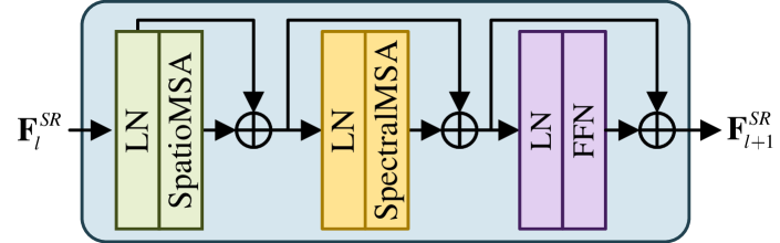
Figure 4: Spatio-Spectral Transformer Layer, where “LN” denotes layer normalization.

Figure 4 illustrates the architecture of one S2TL, which consists of a Spatial Multi-head Self-Attention (SpatioMSA), a Spectral Multi-head Self-Attention (SpectralMSA), and a Feed Forward Network (FFN). SpatioMSA and SpectralMSA learn the interactions of spatial regions and inter-spectra relationships, respectively. To alleviate the computational burden, we adopt the transposed attention [42] in SpectralMSA. SpatioMSA applies the popular window partitioning strategy [22] to reduce the computational complexity. In addition, the gating mechanism [42] is employed in the implementation of FFN.

3.3.3 Noise-Aware Conditional S2TLs

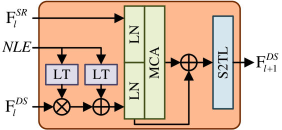
Figure 5: Noise-Aware Conditional Spatio-Spectral Transformer Layer, where “LT” represents linear transform, “LN” denotes layer normalization, and “MCA” is the abbreviation of multi-head cross attention.

To condition the overall model on the hierarchical features of SR stream, we feed $\mathbf{F}_{l}^{SR}$ to the Noise-Aware Conditional S2TLs (NC-S2TLs), each of which is a key building block of the denoising stream. Figure 5 depicts the structure of an NC-S2TL, which takes as input the $NLE$ (a vector), $\mathbf{F}_{l}^{SR}$ and $\mathbf{F}_{l}^{DS}$, where $\mathbf{F}_{l}^{SR}$ and $\mathbf{F}_{l}^{DS}$ have the same spatial resolution. $NLE$ is first transformed and merged with $\mathbf{F}_{l}^{DS}$ with the result subsequently processed with the means of multi-head cross attention (MCA) [4] in order to condition the model on $\mathbf{F}_{l}^{SR}$. As a result, each S2TL learns the spatio-spectral dependencies.

3.4 Progressive Learning

CNN-based restoration models are normally trained on fixed-size image patches. However, training CDFormer on small cropped patches may not appropriately reflect the global image statistics, thereby providing suboptimal performance on full-resolution images when used. To this end, we perform progressive learning where the network is trained on smaller image patches in the early epochs and on gradually larger patches in the later training epochs. The model trained on mixed-size patches via progressive learning shows enhanced performance during testing where images can be of different resolutions (which is a common case in image restoration). The progressive learning strategy behaves in a similar fashion to the curriculum learning process where the network starts with a simpler task and gradually moves to learning a more complex one (where the preservation of fine image structure/textures is required).

To reduce the pressure on the demand of GPU memory, we only train the second half of CDFormer on full-resolution images. The loss function used for such training is defined as follows:

$$\begin{aligned} \mathcal{L}&={\|{\mathbf{X}}-\mathbf{R}{\hat{\mathbf{Z}}_{0}}\|}_{1}+{\|{\mathbf{Y}}-{\hat{\mathbf{Z}}_{0}}\mathbf{D}\|}_{1}+\|\mathbf{Z}_{0}-\hat{\mathbf{Z}}_{0}\|_{1}\\ \hat{\mathbf{Z}}_{0}&=f_{\theta}(\sqrt{\gamma}\mathbf{Z}_{0}+\sqrt{1-\gamma}\boldsymbol{\epsilon},\mathbf{X},\mathbf{Y})\end{aligned},$$ (8)

where $\boldsymbol{\epsilon}\sim\mathcal{N}\left(\mathbf{0},\mathbf{I}\right)$, ($\mathbf{X},\mathbf{Y},\mathbf{Z}$) is sampled from the training set, and the noise schedule about $\gamma$ has been discussed above. The first two terms are designed according to the observation models, while the last one is based on the assumption of Laplace distribution.

4 Experiments

Systematic experiments are herein conducted on four commonly-used public-available HSI-SR datasets to demonstrate the effectiveness of the proposed approach.

4.1 Datasets

Four datasets including CAVE [40], PaviaU [23], Chikusei [41], and HypSen [39] are used in our experiments, with the following details on each.

CAVE:

There are 32 scenes with a spatial size of $512\times 512$ in the CAVE dataset, where we select the first 20 HSIs for training, with the remaining 12 images used for testing. We generate LR-HSIs by Gaussian blur and down-sampling using a factor of 32 as done in [35]. HR-MSIs are acquired by integrating all HR-HSI bands according to the spectral response function of Nikon D700. The original HR-HSIs are treated as ground truth.

PaviaU:

Collected by the University of Pavia, Italy, the original HSI dataset consists of $610\times 340$ pixels in which the top-left $128\times 128$ area is extracted as the test data, with the remaining used for training. Except for water absorption bands, all other 103 bands are chosen for the experiments. Note that the down-sampling factor for the generation of LR-HSIs is four, and the spectral response function is the same as that of the WorldView-3 satellite.

Chikusei:

This dataset consists of 128 bands with a spectral range of 363$nm$ to 1018$nm$ and a spatial resolution of $2517\times 2335$. The original HSI data was taken by an airborne visible and near-infrared imaging sensor over Chikusei, Japan. To alleviate the impact of the back boundary and noise, we crop the center area and remove noise bands. The processed image has a size of $2048\times 2048\times 110$. The top half $1024\times 2048\times 110$ area is selected as the training data, while the rest half is split into eight testing $512\times 512\times 110$ patches. For the production of LR-HSIs and HR-MSIs, this dataset adopts the same processing as with PaviaU.

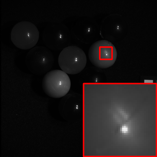
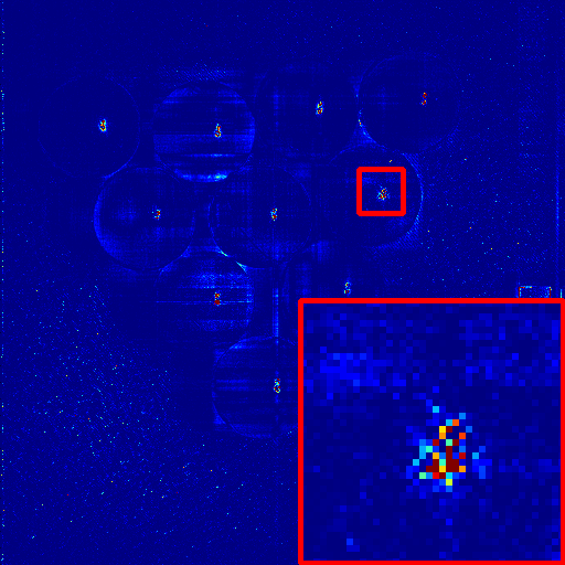
(a) UTV-TD

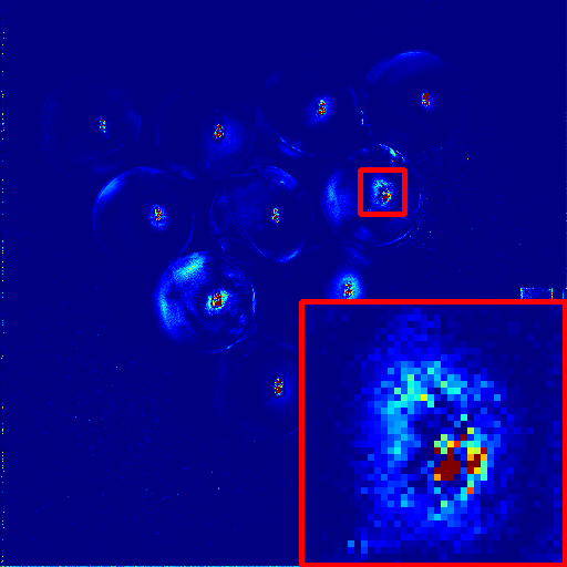
(b) UAL

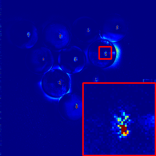
(c) BRResNet

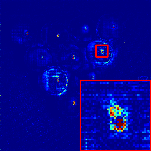
(d) CMHF-Net

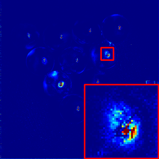
(e) UAL-DMI

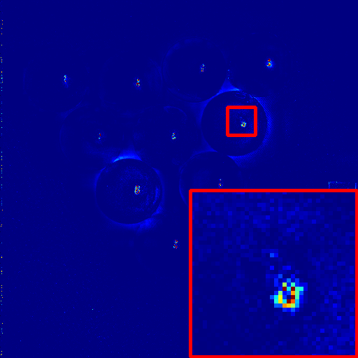
(f) HSR-Diff

(g) Ground truth

Figure 6: Visual quality comparison for fused HSIs of all competing methods on CAVE, where first and second rows show fourth band and corresponding heatmaps (mean squared error), respectively.

(a) UTV-TD

(b) UAL

(c) BRResNet

(d) CMHF-Net

(e) UAL-DMI

(f) HSR-Diff

(g) Ground truth

Figure 7: Visual quality comparison for fused HSIs of all competing methods on PaviaU, where first and second rows show 81st band and corresponding heatmaps (mean squared error), respectively.

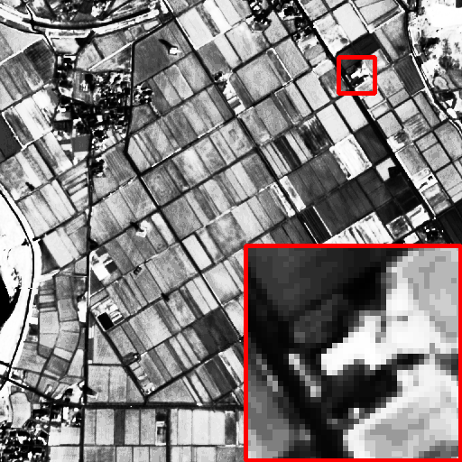
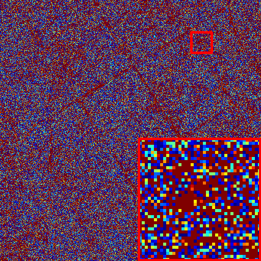
(a) UTV-TD

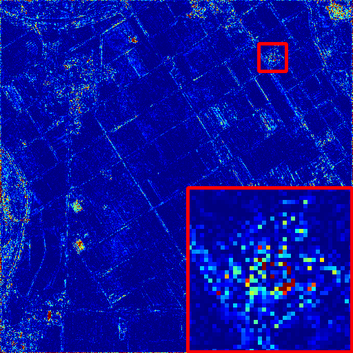
(b) UAL

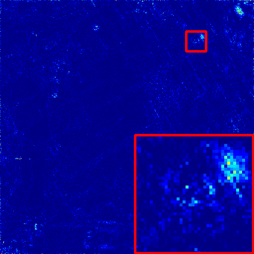
(c) BRResNet

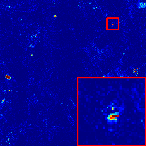
(d) CMHF-Net

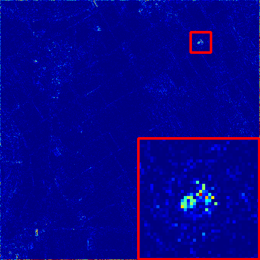
(e) UAL-DMI

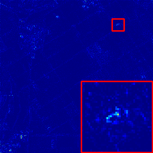
(f) HSR-Diff

(g) Ground truth

Figure 8: Visual quality comparison for fused HSIs of all competing methods on Chikusei, where first and second rows show 67th band and corresponding heatmaps (mean squared error), respectively.

HypSen:

This dataset concerns a real scenario consisting of a 30m-resolution HSI and a 10m-resolution MSI. The Hyperion sensor on the Earth Observing-1 satellite provided the HSI with 242 spectral bands in the spectral range of 400 2500nm, and the MSI with 13 bands was captured by the Sentinel-2A satellite. The blue, green, red, and near-infrared bands of MSI in our experiments are selected due to their high spatial resolution. To eliminate the impact of noise and water absorption, we remove those relevant bands, with 84 bands remaining in the HSI. We crop sub-images of size 250$\times$330 and 750$\times$990 from the Hyperion HSI and Sentinel-2A MSI respectively, in our study, with the pairs of sub-image patches spatially registered.

4.2 Methods Compared and Evaluation Metrics Used

Five state-of-the-art HSI-SR approaches are taken for comparison, including: UTV-TD [37], UAL [44], BRResNet [16], CMHF-Net [35], and UAL-DMI [33]. UTV-TD is a tensor-based technique; UAL, BRResNet, CMHF-Net fall into the category of the DL-based methods; and UAL-DMI can be regarded as an upgraded version of UAL.

Four quantitative quality metrics are employed for performance evaluation, including peak signal-to-noise ratio (PSNR), spectral angle mapper (SAM), erreur relative globale adimensionnelle de synthèse (ERGAS, namely error relative global dimensionless synthesis), and structure similarity (SSIM). The smaller ERGAS and SAM are, the larger PSNR and SSIM are, and the better the fusion result is.

4.3 Implementation Specification

All DL-based methods are trained on the same datasets. For those compared methods, we use the publicly available source codes with default hyper-parameters as given in the corresponding research papers. Our HSR-Diff is implemented on the PyTorch framework. The learnable parameters of the CDFormer are initialized with Kaiming initialization [14] and trained on 2 NVIDIA GeForce GTX 3090s. The number of its channels is set to 256. We utilize the Adam optimizer with $\beta_{1}=0.9$ and $\beta_{2}=0.999$ to optimize the CDFormer. With limited GPU memory, the batch size is set to 4 and 2 for $128^{2}$ and $512^{2}$ images, respectively. It costs 20000 epochs on the CAVE and PaviaU datasets while consuming 5000 epochs on the Chikusei dataset. The learning rate is set as $1\times 10^{-4}$.

4.4 Comparisons with State-of-the-art Methods

In this set of experiments, the evaluations are carried out using the first three datasets listed above without involving the real-world dataset, HypSen (which will be dealt with in the next section).

Qualitative Comparison.

To assess the performance of HSR-Diff qualitatively, we visualize example bands of HSIs in Figures. 6, 7, and 8. It can be seen from these visual results that all compared methods produce satisfactory outcomes. In particular, HSR-Diff generates gives the best result with minor errors since the corresponding MSE (mean squared error) images are much clearer than the others.

Quantitative Comparison.

To further verify the superior performance of the proposed HSR-Diff, quantitative results are presented in Table 1. Note that the performance indices on the CAVE and Chikusei datasets are averaged over all testing samples (12 samples for CAVE and eight samples for Chikusei), respectively. It can be inferred from the results that the proposed HSR-Diff surpasses all competitors with a clear margin on all evaluation metrics.

Dataset	Methods	PSNR $\uparrow$	SSIM $\uparrow$	SAM $\downarrow$	ERGAS $\downarrow$
	UTV-TD	38.66	0.9799	7.98	0.329
	UAL	40.55	0.9933	4.33	0.271
CAVE	BRResNet	41.36	0.9929	4.70	0.250
32$\times$	CMHF-Net	42.54	0.9939	4.69	0.216
	UAL-DMI	42.74	0.9950	3.79	0.213
	HSR-Diff	44.33	0.9951	3.71	0.179
	UTV-TD	44.46	0.9952	1.80	1.236
	UAL	45.42	0.9964	1.54	1.148
PaviaU	BRResNet	45.53	0.9965	1.53	1.111
4$\times$	CMHF-Net	45.77	0.9965	1.50	1.096
	UAL-DMI	45.68	0.9966	1.49	1.113
	HSR-Diff	46.47	0.9977	1.45	1.053
	UTV-TD	48.38	0.9989	0.99	1.303
	UAL	56.18	0.9998	0.49	0.421
Chikusei	BRResNet	56.79	0.9998	0.46	0.366
4$\times$	CMHF-Net	55.99	0.9998	0.50	0.483
	UAL-DMI	56.57	0.9998	0.47	0.387
	HSR-Diff	57.34	0.9999	0.43	0.324

Table 1: Averaged PSNR, SSIM, SAM, and ERGAS of compared methods on CAVE, PaviaU, and Chikusei datasets.

4.5 Ablation Study

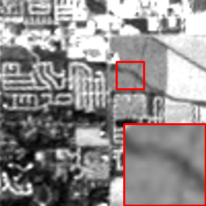
(a) HSI

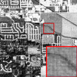
(b) UTV-TD

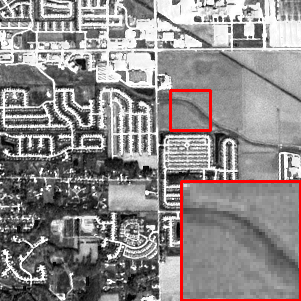
(c) UAL

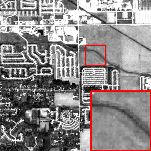
(d) BRResNet

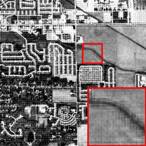
(e) CMHF-Net

(f) UAL-DMI

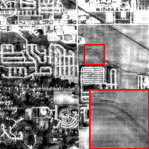
(g) HSR-Diff

Figure 9: Visual fusion results of all competing methods for HypSen.

Effect of conditional diffusion models.

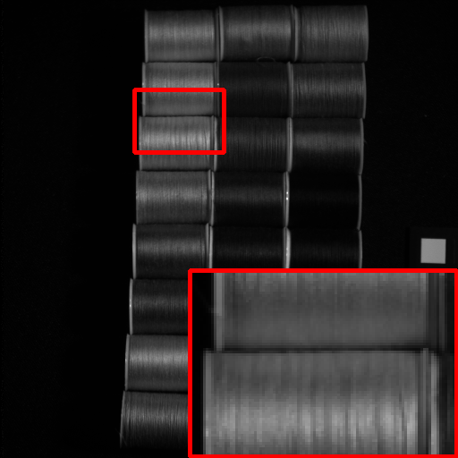
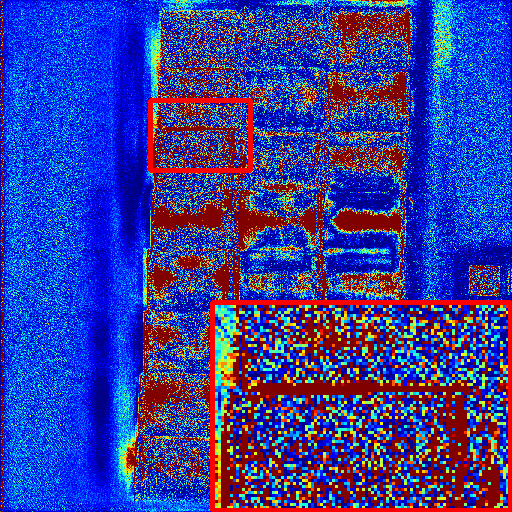
(a) Regression

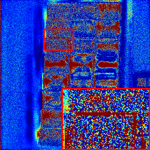
(b) HSR-Diff

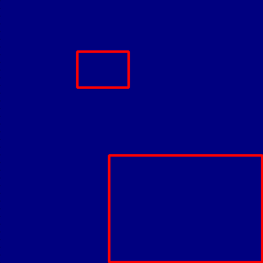
(c) Ground truth

Figure 10: Fusion results (32$\times$) for HSR-Diff and Regression on the thread spools image of CAVE.

Much of the early work on HSI-SR was based on the use of regression models. To compare the effects of the diffusion and regression models, we train regression models containing the CDFormer. Note that the loss function, optimizer, and hyper-parameters are all the same as the conditional diffusion models. Figure 10 presents the fused results and corresponding error maps of utilising HSR-Diff and regression models. As can be seen from the error maps, the HSIs produced by HSR-Diff have less distortion than those by the regression models. This is because HSR-Diff works with a series of iterative refinement steps, facilitating the capture of richer information on data distributions of HR-HSIs.

Effect of CDFormer.

Dataset	Network	PSNR $\uparrow$	SSIM $\uparrow$	SAM $\downarrow$	ERGAS $\downarrow$
CAVE 32$\times$	U-Net	38.84	0.9797	7.32	0.318
	C-w/o-SR	43.74	0.9942	3.94	0.188
	CDFormer	44.33	0.9951	3.71	0.179
PaviaU 4$\times$	U-Net	42.75	0.9962	1.75	1.362
	C-w/o-SR	46.08	0.9976	1.47	1.080
	CDFormer	46.47	0.9977	1.45	1.053
Chikusei 4$\times$	U-Net	47.63	0.9980	1.20	1.794
	C-w/o-SR	56.68	0.9999	0.46	0.425
	CDFormer	57.34	0.9999	0.43	0.324

Table 2: Ablation study on CDFormer.

Recall that CDFormer is conditioned on the hierarchical representations of HR-MSI and LR-HSI via a two-stream architecture. However, alternative outstanding diffusion models [15, 27] that are also excellent for conditional image generation are equipped with CNN-based U-Nets, where degenerated images are concatenated with noisy high-resolution output images. To show the effectiveness of hierarchical representations, we remove the SR stream of CDFormer and name the resulting network “C-w/o-SR”. In addition, we compare CDFormer with a CNN version of CDFormer that replaces all S2TL with convolutional layers and show its results as “CDCNN” in Table 2. The quantitative results show the use of CDFormer performs better than CDCNN, demonstrating the effectiveness of global statistics. Indeed, with the two-stream architecture, CDFormer offers the best results thanks to the use of hierarchical features.

Effect of progressive learning.

Dataset	Methods	PSNR $\uparrow$	SSIM $\uparrow$	SAM $\downarrow$	ERGAS $\downarrow$
CAVE 32$\times$	Fixed	43.17	0.9927	4.99	0.203
	Progressive	44.33	0.9951	3.71	0.179
PaviaU 4$\times$	Fixed	45.06	0.9970	1.63	1.173
	Progressive	46.47	0.9977	1.45	1.053
Chikusei 4$\times$	Fixed	55.92	0.9999	0.50	0.453
	Progressive	57.34	0.9999	0.43	0.324

Table 3: Ablation study on progressive learning.

Progressive learning helps CDFormer to capture long-range dependencies of spatio-spectral information in HR-HSIs. To illustrate the effect of progressive learning, we train the CDFormer with fixed patches ($128^{2}$ for CAVE and Chikusei; $64^{2}$ for PaviaU) with the results shown under the heading of ”Fixed” in Table 3. As can be seen, progressive learning (from $128^{2}$ to $512^{2}$ for CAVE and Chikusei; from $64^{2}$ to $128^{2}$ for PaviaU) provides better results than training with fixed patches.

4.6 Generalization Analysis on Real Dataset

To examine the generalization ability of the implementations following the proposed approach, we test the performance of all competitors on the real-world HypSen dataset [39]. Due to the lack of an ideal HR-HSI to train deep neural networks, we utilize the networks trained on the PaviaU dataset to merge observed LR-HSI and the corresponding HR-MSI. In addition, interpolation is applied to addressing the problem of an inconsistent number of bands between datasets. The fusion results of all compared methods are visualized in Figure 9, from which it can be seen that our method generates rich details, attaining satisfactory quality.

5 Conclusion

In this paper, we have presented the novel HSR-Diff approach that initializes an HR-HSI with pure Gaussian noise and then, iteratively refines it subject to the condition of the LR-HSIs and HR-MSIs of interest. At each step, the noise is removed with CDFormer which exploits the hierarchical representations of HR-MSIs and LR-HSIs rather than the original images. In addition, we employ a progressive learning strategy to maximize the use of the global information of full-resolution images, where CDFormer is trained on small patches in the early epochs with high efficiency while on the global images in the later epochs to obtain the global statistics. Systematic experimental investigations have been conducted, on four public datasets to validate the superior performance of the proposed approach, in comparison with state-of-the-art methods. For future work, we will try to resolve the challenging issue of the relatively low image-generation efficiency of HSR-Diff.

References

- [1] Naveed Akhtar, Faisal Shafait, and Ajmal Mian. Bayesian sparse representation for hyperspectral image super resolution. In Proceedings of the IEEE conference on computer vision and pattern recognition, pages 3631–3640, 2015.
- [2] Martin Arjovsky, Soumith Chintala, and Léon Bottou. Wasserstein generative adversarial networks. In International conference on machine learning, pages 214–223. PMLR, 2017.
- [3] Ricardo Augusto Borsoi, Tales Imbiriba, and José Carlos Moreira Bermudez. Super-resolution for hyperspectral and multispectral image fusion accounting for seasonal spectral variability. IEEE Transactions on Image Processing, 29:116–127, 2019.
- [4] Chun-Fu Richard Chen, Quanfu Fan, and Rameswar Panda. Crossvit: Cross-attention multi-scale vision transformer for image classification. In Proceedings of the IEEE/CVF international conference on computer vision, pages 357–366, 2021.
- [5] Nanxin Chen, Yu Zhang, Heiga Zen, Ron J Weiss, Mohammad Norouzi, and William Chan. Wavegrad: Estimating gradients for waveform generation. In Proceedings of the International Conference on Learning Represent, 2021.
- [6] Zhao Chen, Hanye Pu, Bin Wang, and Geng-Ming Jiang. Fusion of hyperspectral and multispectral images: A novel framework based on generalization of pan-sharpening methods. IEEE Geoscience and Remote Sensing Letters, 11(8):1418–1422, 2014.
- [7] Phuong D Dao, Kiran Mantripragada, Yuhong He, and Faisal Z Qureshi. Improving hyperspectral image segmentation by applying inverse noise weighting and outlier removal for optimal scale selection. ISPRS Journal of Photogrammetry and Remote Sensing, 171:348–366, 2021.
- [8] Renwei Dian, Shutao Li, Anjing Guo, and Leyuan Fang. Deep hyperspectral image sharpening. IEEE transactions on neural networks and learning systems, 29(11):5345–5355, 2018.
- [9] Laurent Dinh, Jascha Sohl-Dickstein, and Samy Bengio. Density estimation using real nvp. arXiv preprint arXiv:1605.08803, 2016.
- [10] Chao Dong, Chen Change Loy, Kaiming He, and Xiaoou Tang. Image super-resolution using deep convolutional networks. IEEE transactions on pattern analysis and machine intelligence, 38(2):295–307, 2015.
- [11] Ying Fu, Tao Zhang, Yinqiang Zheng, Debing Zhang, and Hua Huang. Hyperspectral image super-resolution with optimized rgb guidance. In Proceedings of the IEEE/CVF Conference on Computer Vision and Pattern Recognition, pages 11661–11670, 2019.
- [12] Ian Goodfellow, Jean Pouget-Abadie, Mehdi Mirza, Bing Xu, David Warde-Farley, Sherjil Ozair, Aaron Courville, and Yoshua Bengio. Generative adversarial networks. Communications of the ACM, 63(11):139–144, 2020.
- [13] Ishaan Gulrajani, Faruk Ahmed, Martin Arjovsky, Vincent Dumoulin, and Aaron C Courville. Improved training of wasserstein gans. Advances in neural information processing systems, 30, 2017.
- [14] Kaiming He, Xiangyu Zhang, Shaoqing Ren, and Jian Sun. Delving deep into rectifiers: Surpassing human-level performance on imagenet classification. In Proceedings of the IEEE international conference on computer vision, pages 1026–1034, 2015.
- [15] Jonathan Ho, Ajay Jain, and Pieter Abbeel. Denoising diffusion probabilistic models. Advances in Neural Information Processing Systems, 33:6840–6851, 2020.
- [16] Zi-Rong Jin, Liang-Jian Deng, Tian-Jing Zhang, and Xiao-Xu Jin. Bam: Bilateral activation mechanism for image fusion. In Proceedings of the 29th ACM International Conference on Multimedia, pages 4315–4323, 2021.
- [17] Durk P Kingma and Prafulla Dhariwal. Glow: Generative flow with invertible 1x1 convolutions. Advances in neural information processing systems, 31, 2018.
- [18] Diederik P Kingma and Max Welling. Auto-encoding variational bayes. In Proceedings of the International Conference on Learning Represent, 2013.
- [19] Christian Ledig, Lucas Theis, Ferenc Huszár, Jose Caballero, Andrew Cunningham, Alejandro Acosta, Andrew Aitken, Alykhan Tejani, Johannes Totz, Zehan Wang, et al. Photo-realistic single image super-resolution using a generative adversarial network. In Proceedings of the IEEE conference on computer vision and pattern recognition, pages 4681–4690, 2017.
- [20] Shutao Li, Renwei Dian, Leyuan Fang, and José M Bioucas-Dias. Fusing hyperspectral and multispectral images via coupled sparse tensor factorization. IEEE Transactions on Image Processing, 27(8):4118–4130, 2018.
- [21] Ying Li, Haokui Zhang, and Qiang Shen. Spectral–spatial classification of hyperspectral imagery with 3d convolutional neural network. Remote Sensing, 9(1):67, 2017.
- [22] Ze Liu, Yutong Lin, Yue Cao, Han Hu, Yixuan Wei, Zheng Zhang, Stephen Lin, and Baining Guo. Swin transformer: Hierarchical vision transformer using shifted windows. In Proceedings of the IEEE/CVF International Conference on Computer Vision, pages 10012–10022, 2021.
- [23] Gamba Paolo. Pavia centre and university. https://www.ehu.eus/ccwintco/index.php?titleHypersp ectral_Remote_Sensing_Scenes, 2011.
- [24] Ying Qu, Hairong Qi, and Chiman Kwan. Unsupervised sparse dirichlet-net for hyperspectral image super-resolution. In Proceedings of the IEEE conference on computer vision and pattern recognition, pages 2511–2520, 2018.
- [25] Danilo Rezende and Shakir Mohamed. Variational inference with normalizing flows. In International conference on machine learning, pages 1530–1538. PMLR, 2015.
- [26] Danilo Jimenez Rezende, Shakir Mohamed, and Daan Wierstra. Stochastic backpropagation and approximate inference in deep generative models. In International conference on machine learning, pages 1278–1286. PMLR, 2014.
- [27] Chitwan Saharia, Jonathan Ho, William Chan, Tim Salimans, David J Fleet, and Mohammad Norouzi. Image super-resolution via iterative refinement. IEEE Transactions on Pattern Analysis and Machine Intelligence, 2022.
- [28] Tim Salimans, Andrej Karpathy, Xi Chen, and Diederik P Kingma. Pixelcnn++: Improving the pixelcnn with discretized logistic mixture likelihood and other modifications. In Proceedings of the International Conference on Learning Represent, 2017.
- [29] Yue Shi, Liangxiu Han, Lianghao Han, Sheng Chang, Tongle Hu, and Darren Dancey. A latent encoder coupled generative adversarial network (le-gan) for efficient hyperspectral image super-resolution. IEEE Transactions on Geoscience and Remote Sensing, 60:1–19, 2022.
- [30] Arash Vahdat and Jan Kautz. Nvae: A deep hierarchical variational autoencoder. Advances in Neural Information Processing Systems, 33:19667–19679, 2020.
- [31] Aäron Van Den Oord, Nal Kalchbrenner, and Koray Kavukcuoglu. Pixel recurrent neural networks. In International conference on machine learning, pages 1747–1756. PMLR, 2016.
- [32] Dong Wang, Yunpeng Bai, Chanyue Wu, Ying Li, Changjing Shang, and Qiang Shen. Convolutional lstm-based hierarchical feature fusion for multispectral pan-sharpening. IEEE Transactions on Geoscience and Remote Sensing, 60:1–16, 2022.
- [33] Xiuheng Wang, Jie Chen, and Cédric Richard. Hyperspectral image super-resolution with deep priors and degradation model inversion. In ICASSP 2022-2022 IEEE International Conference on Acoustics, Speech and Signal Processing (ICASSP), pages 2814–2818. IEEE, 2022.
- [34] Qi Wei, José Bioucas-Dias, Nicolas Dobigeon, and Jean-Yves Tourneret. Hyperspectral and multispectral image fusion based on a sparse representation. IEEE Transactions on Geoscience and Remote Sensing, 53(7):3658–3668, 2015.
- [35] Qi Xie, Minghao Zhou, Qian Zhao, Zongben Xu, and Deyu Meng. Mhf-net: An interpretable deep network for multispectral and hyperspectral image fusion. IEEE Transactions on Pattern Analysis and Machine Intelligence, 2022.
- [36] Fengchao Xiong, Jun Zhou, and Yuntao Qian. Material based object tracking in hyperspectral videos. IEEE Transactions on Image Processing, 29:3719–3733, 2020.
- [37] Ting Xu, Ting-Zhu Huang, Liang-Jian Deng, Xi-Le Zhao, and Jie Huang. Hyperspectral image superresolution using unidirectional total variation with tucker decomposition. IEEE Journal of Selected Topics in Applied Earth Observations and Remote Sensing, 13:4381–4398, 2020.
- [38] Xizhe Xue, Haokui Zhang, Bei Fang, Zongwen Bai, and Ying Li. Grafting transformer on automatically designed convolutional neural network for hyperspectral image classification. IEEE Transactions on Geoscience and Remote Sensing, 60:1–16, 2022.
- [39] Jingxiang Yang, Yong-Qiang Zhao, and Jonathan Cheung-Wai Chan. Hyperspectral and multispectral image fusion via deep two-branches convolutional neural network. Remote Sensing, 10(5):800, 2018.
- [40] Fumihito Yasuma, Tomoo Mitsunaga, Daisuke Iso, and Shree K Nayar. Generalized assorted pixel camera: postcapture control of resolution, dynamic range, and spectrum. IEEE transactions on image processing, 19(9):2241–2253, 2010.
- [41] Naoto Yokoya and Akira Iwasaki. Airborne hyperspectral data over chikusei. Space Appl. Lab., Univ. Tokyo, Tokyo, Japan, Tech. Rep. SAL-2016-05-27, 5, 2016.
- [42] Syed Waqas Zamir, Aditya Arora, Salman Khan, Munawar Hayat, Fahad Shahbaz Khan, and Ming-Hsuan Yang. Restormer: Efficient transformer for high-resolution image restoration. In Proceedings of the IEEE/CVF Conference on Computer Vision and Pattern Recognition, pages 5728–5739, 2022.
- [43] Haokui Zhang, Chengrong Gong, Yunpeng Bai, Zongwen Bai, and Ying Li. 3-d-anas: 3-d asymmetric neural architecture search for fast hyperspectral image classification. IEEE Transactions on Geoscience and Remote Sensing, 60:1–19, 2021.
- [44] Lei Zhang, Jiangtao Nie, Wei Wei, Yanning Zhang, Shengcai Liao, and Ling Shao. Unsupervised adaptation learning for hyperspectral imagery super-resolution. In Proceedings of the IEEE/CVF Conference on Computer Vision and Pattern Recognition, pages 3073–3082, 2020.
- [45] Meilin Zhang, Xiongli Sun, Qiqi Zhu, and Guizhou Zheng. A survey of hyperspectral image super-resolution technology. In 2021 IEEE International Geoscience and Remote Sensing Symposium IGARSS, pages 4476–4479. IEEE, 2021.
- [46] Xueting Zhang, Wei Huang, Qi Wang, and Xuelong Li. Ssr-net: Spatial–spectral reconstruction network for hyperspectral and multispectral image fusion. IEEE Transactions on Geoscience and Remote Sensing, 59(7):5953–5965, 2020.
- [47] Ke Zheng, Lianru Gao, Wenzhi Liao, Danfeng Hong, Bing Zhang, Ximin Cui, and Jocelyn Chanussot. Coupled convolutional neural network with adaptive response function learning for unsupervised hyperspectral super resolution. IEEE Transactions on Geoscience and Remote Sensing, 59(3):2487–2502, 2020.