Optimal (degree+1)-Coloring in Congested Clique

Abstract

We consider the distributed complexity of the (degree+1)-list coloring problem, in which each node $u$ of degree $d(u)$ is assigned a palette of $d(u)+1$ colors, and the goal is to find a proper coloring using these color palettes. The (degree+1)-list coloring problem is a natural generalization of the classical $(\Delta+1)$-coloring and $(\Delta+1)$-list coloring problems, both being benchmark problems extensively studied in distributed and parallel computing.

In this paper we settle the complexity of the (degree+1)-list coloring problem in the Congested Clique model by showing that it can be solved deterministically in a constant number of rounds.

1 Introduction

page

Graph coloring problems are among the most extensively studied problems in the area of distributed graph algorithms. In the distributed graph coloring problem, we are given an undirected graph $G=(V,E)$ and the goal is to properly color the nodes of $G$ such that no edge in $E$ is monochromatic. In the distributed setting, the nodes of $G$ correspond to devices that interact by exchanging messages throughout some underlying communication network such that the nodes communicate with each other in synchronous rounds by exchanging messages over the edges in the network. Initially, the nodes do not know anything about $G$ (except possibly for some global parameters, e.g., the number of nodes $n$ or the maximum degree $\Delta$). At the end of computation, each node $v\in V$ should output its color (from a given domain) in the computed coloring. The time or round complexity of a distributed algorithm is the total number of rounds until all nodes terminate.

If adjacent nodes in $G$ can exchange arbitrarily large messages in each communication round (and hence the underlying communication network is equal to the input graph $G$), this distributed model is known as the $\mathsf{LOCAL}$ model [Lin92], and if messages are restricted to $O(\log n)$ bits per edge (limited bandwidth) in each round, the model is known as the $\mathsf{CONGEST}$ model [Pel00]. If we allow all-to-all communication (i.e., the underlying network is a complete graph and thus the communication is independent of the input graph $G$) using messages of size $O(\log n)$ bits then the model is known as the $\mathsf{CongestedClique}$ model [LPPP05].

The most fundamental graph coloring problem in distributed computing (studied already in the seminal paper by Linial [Lin92] that introduced the $\mathsf{LOCAL}$ model) is $(\Delta+1)$-coloring: assuming that the input graph $G$ is of maximum degree $\Delta$, the objective is to properly color nodes of $G$ using $\Delta+1$ colors from $\{1,2,\dots,\Delta+1\}$. The $(\Delta+1)$-coloring problem can be easily solved by a sequential greedy algorithm, but the interaction between local and global aspects of graph coloring create some non-trivial challenges in a distributed setting. The problem has been used as a benchmark to study distributed symmetry breaking in graphs, and it is at the very core of the area of distributed graph algorithms. $(\Delta+1)$-list coloring is a natural generalization of $(\Delta+1)$-coloring: each node has an arbitrary palette of $\Delta+1$ colors, and the goal is to compute a legal coloring in which each node is assigned a color from its own palette. A further generalization is the (degree+1)-list coloring (D1LC) problem, which is the same as the $(\Delta+1)$-list coloring problem except that the size of each node $v$’s palette is $d(v)+1$, which might be much smaller than $\Delta+1$. These three problems always have a legal coloring (easily found sequentially using a greedy approach), and the main challenge in the distributed setting is to find the required coloring in as few rounds as possible.

These three graph coloring problems have been studied extensively in distributed computing, though $(\Delta+1)$-coloring, as the simplest, has attracted most attention. However, one can also argue that (degree+1)-list coloring, as the most versatile, is more algorithmically fundamental than $(\Delta+1)$-coloring. For example, given a partial solution to a $(\Delta+1)$-coloring problem, the remaining coloring problem on the uncolored nodes is an instance of the (degree+1)-list coloring problem. The (degree+1)-list coloring problem is self-reducible: after computing a partial solution to a (degree+1)-list coloring problem, the remaining problem is still a (degree+1)-list coloring problem. It also naturally appears as a subproblem in more constrained coloring problems: for example, it has been used as a subroutine in distributed $\Delta$-coloring algorithms (see, e.g., [FHM23]), in efficient $(\Delta+1)$-coloring and edge-coloring algorithms (see, e.g., [Kuh20]), and in other graph coloring applications (see, e.g. [BE19]).

Following an increasing interest in the distributed computing community for (degree+1)-list coloring, it is natural to formulate a central challenge relating it to $(\Delta+1)$-coloring:

Can we solve the (degree+1)-list coloring problem in asymptotically the same round complexity as the simpler $(\Delta+1)$-coloring problem?

This challenge has been elusive for many years and only in the last year the affirmative answer was given for randomized algorithms in $\mathsf{LOCAL}$ and $\mathsf{CONGEST}$. First, in a recent breakthrough, Halldórsson, Kuhn, Nolin, and Tonoyan [HKNT22] gave a randomized $O(\log^{3}\log n)$-round distributed algorithm for (degree+1)-list coloring in the $\mathsf{LOCAL}$ model, matching the state-of-the-art complexity for the $(\Delta+1)$-coloring problem [CLP20, RG20]. This has been later extended to the $\mathsf{CONGEST}$ model by Halldórsson, Nolin, and Tonoyan [HNT22], who designed a randomized algorithm for (degree+1)-list coloring that runs in $O(\log^{5}\log n)$-round, matching the state-of-the-art complexity for the $(\Delta+1)$-coloring problem in $\mathsf{CONGEST}$ [HKMT21].

The main contribution of our paper is a complete resolution of this challenge in the $\mathsf{CongestedClique}$ model, and in fact, even for deterministic algorithms. We settle the complexity of the (degree+1)-list coloring problem in $\mathsf{CongestedClique}$ by showing that it can be solved deterministically in a constant number of rounds.

Theorem 1.1.

page There is a deterministic $\mathsf{CongestedClique}$ algorithm which finds a (degree+1)-list coloring of any graph in a constant number of rounds.

1.1 Background and Related Works

page

The distributed graph coloring problems have been extensively studied in the last three decades, starting with a seminal paper by Linial [Lin92] that introduced the $\mathsf{LOCAL}$ model and originated the area of local graph algorithms. Since the $(\Delta+1)$-coloring problem can be solved by a simple sequential greedy algorithm, but it is challenging to be solved efficiently in distributed (and parallel) setting, the $(\Delta+1)$-coloring problem became a benchmark problem for distributed computing and a significant amount of research has been devoted to the study of these problems in all main distributed models: $\mathsf{LOCAL}$, $\mathsf{CONGEST}$, and $\mathsf{CongestedClique}$. The monograph [BE13] gives a comprehensive description of many of the earlier results.

It is known from research on parallel algorithms that $(\Delta+1)$-coloring can be computed in $O(\log n)$ rounds by randomized algorithms in the $\mathsf{LOCAL}$ model [ABI86, Lub86]. Linial [Lin92] observed that for smaller values of $\Delta$, one can do better: he showed that it is possible to deterministically color arbitrary graphs of maximum degree $\Delta$ with $O(\Delta^{2})$ colors in $O(\log^{*}n)$ rounds; this can be easily extended to obtain a deterministic $\mathsf{LOCAL}$ algorithm for $(\Delta+1)$-coloring that runs in $O(\Delta^{2}+\log^{*}n)$ rounds, and thus in bounded degree graphs, a $(\Delta+1)$-coloring can be computed in $O(\log^{*}n)$ rounds. These results have since been improved for general values of $\Delta$: the current state-of-the-art for the $(\Delta+1)$-coloring problem in $\mathsf{LOCAL}$ is $O(\log^{3}\log n)$ rounds for randomized algorithms [CLP20, RG20] and $O(\log^{2}\Delta\cdot\log n)$ for deterministic algorithms [GK21]. Furthermore, the fastest algorithms mentioned above can be modified to work also for the more general $(\Delta+1)$-list coloring problem in the $\mathsf{LOCAL}$ model. (In fact, many of those algorithms critically rely on this problem as a subroutine.)

For the $\mathsf{CONGEST}$ model, the parallel algorithms mentioned above [ABI86, Lub86] can be implemented in the $\mathsf{CONGEST}$ model to obtain randomized algorithms for both the $(\Delta+1)$-coloring and $(\Delta+1)$-list coloring problems that run in $O(\log n)$ rounds. Only recently this bound has been improved for all values of $\Delta$: In a seminal paper, Halldórsson et al. [HKMT21] designed a randomized $\mathsf{CONGEST}$ algorithm that solves the $(\Delta+1)$-coloring and $(\Delta+1)$-list coloring problems in $O(\log^{5}\log n)$ rounds. For deterministic computation, the best $\mathsf{LOCAL}$ algorithm [GK21] works directly in $\mathsf{CONGEST}$, running in $O(\log^{2}\Delta\cdot\log n)$ rounds.

As for the lower bounds, one of the first results in distributed computing was a lower bound in $\mathsf{LOCAL}$ of $\Omega(\log^{*}n)$ rounds for computing an $O(1)$-coloring of a graph of maximum degree $\Delta=2$, shown by Linial [Lin92] for deterministic algorithms, and by Naor [Nao91] for randomized ones. Stubbornly, the $\Omega(\log^{*}n)$ rounds is still the best known lower bound for the $(\Delta+1)$-coloring problem in $\mathsf{LOCAL}$ and $\mathsf{CONGEST}$.

We can do better for the $\mathsf{CongestedClique}$ model. After years of gradual improvements, Parter [Par18] exploited the $\mathsf{LOCAL}$ shattering approach from [CLP20] to give the first sublogarithmic-time randomized $(\Delta+1)$-coloring algorithm for $\mathsf{CongestedClique}$, which runs in $O(\log\log\Delta\cdot\log^{*}\Delta)$ rounds. This bound has been later improved Parter and Su [PS18] to $O(\log^{*}\Delta)$ rounds. Finally, Chang et al. [CFG⁺19] settled the randomized complexity of $(\Delta+1)$-coloring (and also for $(\Delta+1)$-list coloring) and obtained a randomized $\mathsf{CongestedClique}$ algorithm that runs in a constant number of rounds. This result has been later simplified and turned into a deterministic constant-round $\mathsf{CongestedClique}$ algorithm by Czumaj et al. [CDP21d].

(degree+1)-list coloring ($\mathsf{D1LC}$).

The $\mathsf{D1LC}$ problem in distributed setting has been studied both on its own, and also as a tool in designing distributed algorithms for other coloring problems, like $(\Delta+1)$-coloring, $(\Delta+1)$-list coloring, and $\Delta$-coloring. The problem is not easier than the $(\Delta+1)$-coloring and the $(\Delta+1)$-list coloring problems, and the difficulty of dealing with vertices having color palettes of significantly different sizes makes the problem more challenging. As the result, until very recently the obtained complexity bounds have been significantly weaker than the bounds for the $(\Delta+1)$-coloring problem, see, e.g., [BKM20, FHK16, Kuh20]. This changed last year, when in a recent breakthrough Halldórsson et al. [HKNT22] gave a randomized $O(\log^{3}\log n)$-round distributed algorithm for $\mathsf{D1LC}$ in the $\mathsf{LOCAL}$ distributed model. Observe that this bound matches the state-of-the-art complexity for the (easier) $(\Delta+1)$-coloring problem [CLP20]. This work has been later extended to the $\mathsf{CONGEST}$ model by Halldórsson et al. [HNT22], who designed a randomized $\mathsf{CONGEST}$ algorithm for $\mathsf{D1LC}$ that runs in $O(\log^{5}\log n)$ rounds. Similarly as for the $\mathsf{LOCAL}$ model, this bound matches the state-of-the-art complexity for the $(\Delta+1)$-coloring problem in $\mathsf{CONGEST}$ [HKMT21].

Specifically for the $\mathsf{CongestedClique}$ model, the only earlier $\mathsf{D1LC}$ result we are aware of is by Bamberger et al. [BKM20], who extended their own $\mathsf{CONGEST}$ algorithm for the problem to obtain a deterministic $\mathsf{D1LC}$ algorithm requiring $O(\log\Delta\log\log\Delta)$ rounds in $\mathsf{CongestedClique}$. However, the randomized state-of-the-art $\mathsf{D1LC}$ bound in the $\mathsf{CongestedClique}$ model follows from the aforementioned $O(\log^{5}\log n)$-round $\mathsf{CONGEST}$ algorithm by Halldórsson et al. [HNT22], which works directly in $\mathsf{CongestedClique}$. This should be compared with the state-of-the-art $O(1)$-round $\mathsf{CongestedClique}$ algorithms for $(\Delta+1)$-coloring [CFG⁺19, CDP21d].

Recent work in $\mathsf{D1LC}$ on $\mathsf{MPC}$.

Various coloring problems have been also studied in a related model of parallel computation, the so-called Massively Parallel Computation ($\mathsf{MPC}$) model. The $\mathsf{MPC}$ model, introduced by Karloff et al. [KSV10], is now a standard theoretical model for parallel algorithms. The $\mathsf{MPC}$ model with $O(n)$ local space and $n$ machines is essentially equivalent to the $\mathsf{CongestedClique}$ model (see, e.g., [BDH18, HP15]), and this implies that many $\mathsf{MPC}$ algorithms can be easily transferred to the $\mathsf{CongestedClique}$ model. (However, this relationship requires that the local space of $\mathsf{MPC}$ is $O(n)$, not more.)

Both the $(\Delta+1)$-coloring and $(\Delta+1)$-list coloring problems have been studied in $\mathsf{MPC}$ extensively (see, e.g., [BKM20, CDP21d] for linear local space $\mathsf{MPC}$ and [BKM20, CFG⁺19, CDP21c] for sublinear local space $\mathsf{MPC}$). We are aware only of a few works for the $\mathsf{D1LC}$ problem on $\mathsf{MPC}$, see [BKM20, CCDM23, HKNT22]. The work most relevant to our paper is the result of Halldórsson et al. [HKNT22]. They give a constant-round $\mathsf{MPC}$ algorithm assuming the local $\mathsf{MPC}$ space is slightly superlinear, i.e., $\Omega(n\log^{4}n)$ [HKNT22, Corollary 2]. This result relies on the palette sparsification approach due to Alon and Assadi [AA20] (see also [ACK19]) to the $\mathsf{D1LC}$ problem, which reduces the problem to a sparse instance of size $O(n\log^{4}n)$; hence, on an $\mathsf{MPC}$ with $\Omega(n\log^{4}n)$ local space one can put the entire graph on a single $\mathsf{MPC}$ machine and then solve the problem in a single round. Given the similarity of $\mathsf{CongestedClique}$ and the $\mathsf{MPC}$ model with linear local space, one could hope that the use of “slightly superlinear” $\mathsf{MPC}$ local space in [HKNT22] can be overcome and the approach can allow the problem to be solved in linear local space, resulting in a $\mathsf{CongestedClique}$ algorithm with a similar performance. Unfortunately, we do not think this is the case. One argument supporting this challenge is that the hardest instances for $\mathsf{D1LC}$ algorithms are sparse graphs, and in a typical case sparsification and reduction to low-degree graphs do not seem to help. Further, we have recently seen a similar situation in $(\Delta+1)$-coloring. The palette sparsification by Assadi et al. [ACK19] trivially implies a constant-round $\mathsf{MPC}$ algorithm for $(\Delta+1)$-coloring with local space $\Omega(n\log^{2}n)$, but does not give a constant-round algorithm for $(\Delta+1)$-coloring in $\mathsf{CongestedClique}$. Only by using a fundamentally different approach Chang et al. [CFG⁺19] and then (deterministically) Czumaj et al. [CDP21b] obtained constant-round $(\Delta+1)$-coloring algorithms in $\mathsf{CongestedClique}$. Hence, despite having a constant-round algorithm for $\mathsf{D1LC}$ in $\mathsf{MPC}$ with local space $\Omega(n\log^{4}n)$, possibly a different approach than palette sparsification is needed to achieve a similar performance for $\mathsf{D1LC}$ in $\mathsf{CongestedClique}$.

Derandomization tools for distributed coloring algorithms.

In our paper we rely on a recently developed general scheme for derandomization in the $\mathsf{CongestedClique}$ model (and used also extensively in the $\mathsf{MPC}$ model) by combining the methods of bounded independence with efficient computation of conditional expectations. This method was first applied by Censor-Hillel et al. [CHPS20], and has since been used in several other works for graph coloring problems, (see, e.g., [CDP21d, Par18]), and for other problems in $\mathsf{CongestedClique}$ and $\mathsf{MPC}$.

The underlying idea begins with the design of a randomized algorithm using random choices with only limited independence, e.g., $O(1)$-wise-independence. Then, each round of the randomized algorithm can be simulated by giving all nodes a shared random seed of $O(\log n)$ bits. Next, the nodes deterministically compute a seed which is at least as good as a random seed is in expectation. This is done by using an appropriate estimation of the local quality of a seed, which can be aggregated into a global measure of the quality of the seed. Combining this with the techniques of conditional expectation, pessimistic estimators, and bounded independence, this allows selection of the bits of the seed “batch-by-batch,” where each batch consists of $O(\log n)$ bits. Once all bits of the seed are computed, we can used it to simulate the random choices of that round, as it would have been performed by a randomized algorithm. A more detailed explanation of this approach is given in subsec:mpc_derandomization.

1.2 Technical Overview

page

The core part of our constant-round deterministic $\mathsf{CongestedClique}$ $\mathsf{D1LC}$ algorithm (BucketColor, alg:bucketcolor) does not follow the route of recent $\mathsf{D1LC}$ algorithms for $\mathsf{LOCAL}$ and $\mathsf{CONGEST}$ due to Halldórsson et al. [HKNT22, HNT22]. Instead, it uses fundamentally different techniques, extending the approach developed recently in a simple deterministic $O(1)$-round $\mathsf{CongestedClique}$ algorithm for $(\Delta+1)$-list coloring of Czumaj, Davies, and Parter [CDP21d]. Their $(\Delta+1)$-list coloring algorithm works by partitioning nodes and colors into $\Delta^{\varepsilon}$ buckets, for a small constant $\varepsilon$. (This partitioning is initially at random, but then it is derandomized using the method of conditional expectations). The nodes are distributed among all buckets, except for one “leftover” bucket, which is left without colors and is set aside to be colored later. Then, each node’s palette is restricted to only the colors assigned to its bucket (except those in the leftover bucket, whose palettes are not restricted). This ensures that nodes in different buckets have entirely disjoint palettes, and therefore edges between different buckets can be removed from the graph, since they would never cause a coloring conflict. One important property is that nodes still have sufficient colors when their palettes were restricted in this way. This is achieved in [CDP21d] using two main arguments: firstly, the fact that colors are distributed among one fewer buckets than nodes provided enough ‘slack’ to ensure that with reasonably high probability, a node would receive more colors than neighbors in its bucket. Secondly, the few nodes that do not satisfy this property induce a small graph (of size $O(n)$), and therefore can be collected onto a single network node and color separately.

Using the approach from [CDP21d] sketched above, a $(\Delta+1)$-list coloring instance can be reduced into multiple smaller $(\Delta+1)$-list coloring instances (i.e., on fewer nodes and with a new, lower maximum degree) that are independent (since they had disjoint palettes), and so can be solved in parallel without risking coloring conflicts. The final part of the analysis of [CDP21d] was to show that, after recursively performing this bucketing process $O(1)$ times, these instances are of $O(n)$ size and therefore they could be collected to individual nodes and solved in a constant number of rounds in $\mathsf{CongestedClique}$.

There are major barriers to extending this approach to (degree+1)-list coloring. Crucially, it required the number of buckets to be dependent on $\Delta$, and all nodes’ palette sizes to be at least $\Delta$. Dividing nodes among too few buckets would cause the induced graphs to be too large, and the algorithm would not terminate in $O(1)$ rounds; using too many buckets would fail to provide nodes with sufficient colors in their bucket. In the $\mathsf{D1LC}$ problem, we no longer have a uniform bound on palette size, so it is unclear how to perform this bucketing.

Our first major conceptual change is that, rather than simply partitioning among a number (dependent on $\Delta$) of equivalent buckets, we instead use a tree-structured hierarchy of buckets, with the $O(\log\log\Delta)$ levels in the hierarchy corresponding to doubly-exponentially increasing degree ranges (see Figure 1). Nodes with degree $d(v)$ will be mapped to a bucket in a level containing (very approximately) $d(v)^{0.7}$ buckets. Colors will be mapped to a top-level (leaf) bucket, but will also be assigned to every bucket on the leaf-root path in the bucket tree (see Figure 2). We can therefore discard all edges between different buckets that do not have an ancestor-descendant relationship, since these buckets will have disjoint palettes.

This change allows nodes to be bucketed correctly according to their own degree. However, it introduces several new difficulties:

• We no longer get a good bound on the number of lower-degree neighbors of a node $v$ that may share colors with it. We can only hope to prove that $v$ receives enough colors relative to its higher (or same)-degree neighbors.

• The technique of having a leftover bucket which is not assigned colors no longer works to provide slack (nor even makes sense - we would need a leftover bucket at every level, but, for example, level $0$ only contains one bucket).

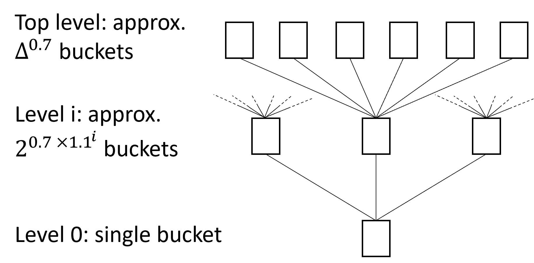
Figure 1: Bucket structurepage

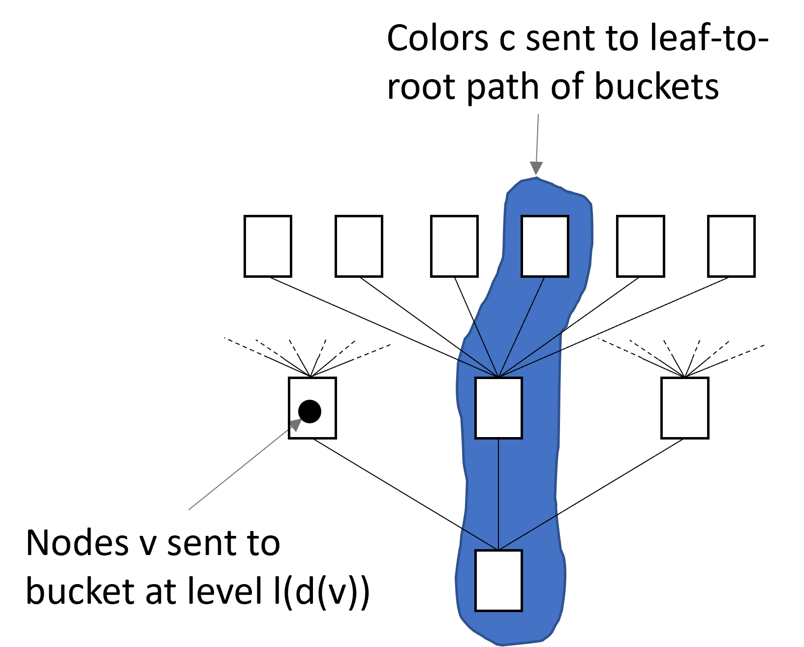
Figure 2: Partitioning nodes and colorspage

In order to cope with these challenges, firstly, we employ the observation that if we were to greedily color in non-increasing order of degree, we would require nodes to have a palette size of $d^{+}(v)+1$ (where $d^{+}(v)$ is the number of $v$’s neighbors of equal or higher degree), rather that $d(v)+1$ (since $d^{+}(v)$ of $v$’s neighbors will have been colored at the point $v$ is considered). Therefore, we argue that we can still show that the graph is colorable even though our bucketing procedure may leave nodes with many more lower-degree neighbors than palette colors. (It is not necessarily clear how to find such a coloring in a parallel fashion, but in our analysis, we will be able to address this issue.)

This observation also helps us with the problem of generating slack without a leftover bucket. We show that, since lower-order neighbors are now effectively providing slack, only nodes with very few lower-order neighbors may not receive enough colors (relative to higher-order neighbors) in their bucket. It transpires that we can generate slack for these nodes prior to BucketColor via derandomizations of fairly standard procedures (ColorTrial, alg:colortrialrand, and Subsample, alg:subsamplerand). The randomized bases for all these procedures would inevitably result in some nodes failing to meet the necessary properties for the next stage. To overcome this, we derandomize all of these procedures, using the method of conditional expectations. As well as making the algorithm deterministic, this has the important property of ensuring that failed nodes form an $O(n)$-size induced graph, which can be easily dealt with later.

Having solved the problem of slack for the bucketing process (by showing that nodes have received palettes of size at least $d^{+}(v)+1$ within their buckets), it remains to find a parallel analog to greedily coloring in non-increasing order of degree. Our approach here is to repeatedly move all nodes from their current bucket to a child of that bucket in the bucket tree (which further restricts their neighborhood and available palette). We show that, by correct choice of bucket and order of node consideration, we will always be able to find child buckets such that each node still has palette size at least $d^{+}(v)+1$ according to the new bucket assignment. We also show that, after $O(1)$ iterations of this process, nodes only have one palette color in their bucket, and zero higher-order neighbors. Then, all nodes can safely color themselves this palette color, and the coloring is complete.

The overall structure of the main algorithm Color (alg:mainrand) is more complicated, since Subsample produces a graph $G^{\prime}$ of leftover nodes that are deferred to be colored later. We recursively run alg:mainrand on this graph $G^{\prime}$, and show that it is sufficiently smaller than the original input graph that after $O(1)$ recursive calls, the remaining graph has size $O(n)$ and can be collected and solved on a single network node.

If we combine all these tools together then we will be able to obtain a randomized $\mathsf{CongestedClique}$ algorithm that finds a (degree+1)-list coloring of any graph in $O(1)$ rounds. Using method of conditional expectation using bounded-independence hash function (see subsec:mpc_derandomization-2.4), each randomized step of our algorithm can be derandomized.

2 Preliminaries

page

The main model considered in this paper is $\mathsf{CongestedClique}$, as introduced by Lotker et al. [LPPP05]. It is a variant of $\mathsf{CONGEST}$, in which nodes can send a message of size $O(\log n)$ to each neighboring node in the graph in each communication round: the difference is that $\mathsf{CongestedClique}$ allows all-to-all communication, and hence the underlying communication network is a complete graph on the nodes $V$. In particular, this allows the communication to be performed between all pairs of nodes rather than being restricted to the edges of the input graph. $\mathsf{CongestedClique}$ has been introduced as a theoretical model to study overlay networks: an abstraction that separates the problems emerging from the topology of the communication network from the problems emerging from the structure of the problem at hand. It allows us to study a model in which each pair of nodes can communicate, and we do not consider any details of how this communication is executed by the underlying network.

The degree+1 list coloring ($\mathsf{D1LC}$) problem is for a given graph $G=(V,E)$ on $n$ nodes and given color palettes $\Psi(u)$ assigned to each node $u\in V$, such that $\left|\Psi(u)\right|\geq d(u)+1$, the objective to find a proper coloring of nodes in $G$ such that each node as assigned to a color from its color palette (and, as in proper coloring, no edge in $G$ is monochromatic). The input to the $\mathsf{D1LC}$ problem in $\mathsf{CongestedClique}$ is a graph $G$, where each node $v$ of $G$ has assigned a network node and this network node knows $\Psi(v)$ and all neighbors of $v$ in $G$.

A useful property of the $\mathsf{CongestedClique}$ model is that thanks to the constant round routing algorithm of Lenzen [Len13], information can be redistributed essentially arbitrarily in the communication network, so there is no need to associate the computational entities with nodes in the input graph $G$. (This is in stark contrast to the related LOCAL and CONGEST distributed models in which the link between computation and input graph locality is integral.) In particular, this allows us to collect graphs of size $O(n)$ on a single node in $O(1)$ rounds. Because of this “decoupling” of the computation from the input graph, where appropriate we will distinguish the nodes in their roles as computational entities (“network nodes”) from the nodes in the input graph (“graph nodes”).

2.1 Notation

page

For $k\in\mathbb{N}$ we let $[k]:=\{1,\dots,k\}$. We consider a graph $G=(V(G),E(G))$ with $V(G)$ as the node set and $E(G)$ as the edge set. The size of a graph $G$ refers to the number of edges in $G$ and is denoted by $|G|$. The set of neighbors of a node $v$ is denoted by $N_{G}(v)$ and the degree of a node $v$ is denoted by $d_{G}(v)$. The maximum degree of any node in $G$ is denoted by $\Delta_{G}$. For any node $v$, we partition its neighbors into two sets $N_{G}^{+}(v):=\{u\in N_{G}(v):d_{G}(u)\geq d_{G}(v)\}$ and $N_{G}^{-}(v):=\{u\in N_{G}(v):d_{G}(u)<d_{G}(v)\}$, and let $d_{G}^{+}(v):=|N_{G}^{+}(v)|$ and $d_{G}^{-}(v):=|N_{G}^{-}(v)|$. When $G$ is clear from the context, we suppress $G$ from the subscripts of the notation.

For the coloring problem, for a node $v$, $\Psi_{G}(v)$ denotes the list of colors in the color palette of $v$ and $p_{G}(v):=|\Psi_{G}(v)|$. As we proceed in coloring the nodes of the input graph $G$ the graph will be changing and the color palettes of the nodes may also change. We will ensure that at any moment, if $G$ denotes the current graph then we have $p_{G}(v)\geq d_{G}(v)+1$. We use $\mathcal{C}$ to denote the set of all colors present in the palette of any node (in a given moment).

For binary strings $a$ and $a^{\prime}$ in $\{0,1\}^{*}$, $a\sqsubseteq a^{\prime}$ denotes that $a$ is a prefix of $a^{\prime}$, and $a\sqsubset a^{\prime}$ denotes that it is a strict prefix of $a^{\prime}$. Furthermore, $a^{\prime}\sqsupseteq a$ iff $a\sqsubseteq a^{\prime}$, and $a^{\prime}\sqsupset a$ iff $a\sqsubset a^{\prime}$.

2.2 Derandomization in $\mathsf{CongestedClique}$

page

The method of conditional expectations using bounded-independence hash functions is a nowadays classical technique for the derandomization of algorithms [ES73, Lub93, MNN94, Rag88]. Starting with the recent work of Censor-Hillel et al. [CHPS20], this approach has been found very powerful also in the setting of distributed and parallel algorithms, see e.g., [BKM20, CDP21a, CDP21b, CDP21c, CDP21d, DKM19, FGG22, GK18, Par18].

This technique requires that we show that our randomized algorithm can be made to work in expectation using only bounded-independence. It is known that small families of bounded-independence hash functions exist, and that hash functions in these families can be specified by a short seed. It is also known that such a family must contain a hash function which beats the expectation due to the probabilistic method. Using these facts, we can perform an efficient search for a hash function which beats the expectation by iteratively setting a larger and larger prefix of the seed of the hash function.

In this section we first give some useful lemmas regarding $O(1)$-wise independence and the existence of small families of $O(1)$-wise independent hash functions, and then we give a formal description of the method of conditional expectations and how it is implemented in the $\mathsf{CongestedClique}$ model.

2.3 Bounded Independence

page

Our algorithm will be finding a hash function of sufficient quality from a family of $O(1)$-independent hash functions. In the following, we recall the standard notions of $k$-wise independent hash functions and $k$-wise independent random variables. Then, we recall that we can construct small families of bounded-independence hash functions, and that each hash function in this family can be specified by a short seed. Finally, we state a concentration inequality (for $k$-wise independent random variables) that will be used in the analysis of our algorithm while bounding the probabilities of some desired events.

Definition 2.1.

Let $k\geq 2$ be an integer. A set $\{X_{1},\ldots,X_{n}\}$ of $n$ random variables taking values in $S$ are said to be $k$-wise independent if for any $I\subset[n]$ with $|{I}|\leq k$ and any $x_{i}\in S$ for $i\in I$, we have

$$\mathbf{Pr}\left[\bigwedge_{i\in[k]}X_{i}=x_{i}\right] =\prod_{i=1}^{k}\mathbf{Pr}\left[X_{i}=x_{i}\right]\enspace.$$

Definition 2.2.

A family of hash functions $\mathcal{H}=\{h:X\rightarrow Y\}$ is said to be $k$-wise independent if $\{h(x):x\in X\}$ are $k$-wise independent when $h$ is drawn uniformly at random from $\mathcal{H}$.

We use the property that small families of $O(1)$-wise independent hash functions can be constructed, and each hash function in such a family can be specified with a small number of bits:

Remark 2.3.

page For all positive integers $c_{1},c_{2}$, there is a family of $k$-wise independent hash functions $\mathcal{H}=\{h:[n^{c_{1}}]\rightarrow[n^{c_{2}}]\}$ such that each function from $\mathcal{H}$ can be specified using $O(k\log n)$ bits.

We finish this subsection by giving some useful tail bounds for $O(1)$-wise independent random variables.

Lemma 2.4 (Lemma 2.3 of [BR94]).

page Let $k\geq 4$ be an even integer. Suppose $X_{1},\dots,X_{n}$ are $k$-wise independent random variables taking values in $[0,1]$. Let $X=X_{1}+\dots+X_{n}$, and $\mu=\mathbf{E}\left[X\right]$ is the expectation of $X$. If $\mu\geq 1000$, then:

$$\mathbf{Pr}\left[|X-\mu|\geq A\right] \leq 8\left(\frac{k\mu+k^{2}}{A^{2}}\right)^{k/2}\enspace.$$

We will always use lem:conc with $k=100$ and $\mu\geq 1000$, giving the following special case:

Corollary 2.5.

page Suppose $X_{1},\dots,X_{n}$ are $100$-wise independent random variables taking values in $[0,1]$. Let $X=X_{1}+\dots+X_{n}$, and $\mu=\mathbf{E}\left[X\right]$ is the expectation of $X$. Then,

$$\mathbf{Pr}\left[|X-\mu|\geq A\right] \leq\left(\frac{111\mu}{A^{2}}\right)^{50}\enspace.$$

Proof.

By lem:conc,

$$\mathbf{Pr}\left[|X-\mu|\geq A\right] \leq 8\left(\frac{100\mu+10000}{A^{2}}\right)^{50}\leq 8\left(\frac{110\mu}{A^{2}}\right)^{50}\leq\left(\frac{111\mu}{A^{2}}\right)^{50}\enspace.\qed$$

2.4 The Method of Conditional Expectations

page

We now describe in more detail the method of conditional expectations and its implementation in $\mathsf{CongestedClique}$. We briefly recall the setup to the problem: we have a randomized algorithm which “succeeds” if a “bad” outcome occurs for less than some number $T$ of nodes. This algorithm succeeds in expectation using bounded-independence randomness. We would like to derandomize this algorithm. In order to achieve this, given a family of $O(1)$-wise independent hash functions $\mathcal{H}$, we need to find a “good” hash function $h^{*}\in\mathcal{H}$ which solves our problem, when used to make decisions for nodes instead of randomness.

First, we define some cost function $f:\mathcal{H}\times V\rightarrow\{0,1\}$ such that $f(h,v)=1$ if the node $v$ has a “bad” outcome when $h$ is the selected hash function, and $f(h,v)=0$ if the outcome is “good”. We further define $F(h)=\sum_{v\in V}f(h,v)$ as the total cost of the hash function $h$: i.e., the number of bad nodes when $h$ is the selected hash function. Finally, we use $\mathbf{E}_{h\in\mathcal{H}}[F(h)]$ to denote the expected value of $F(h)$ when $h$ is drawn uniformly at random from $\mathcal{H}$.

To successfully derandomize our algorithm, we need to find a hash function $h^{*}\in\mathcal{H}$ such that $F(h^{*})\leq T$. We need the following conditions to hold for our derandomization to work:

• $\mathbf{E}_{h\in\mathcal{H}}[F(h)]\leq T$ (i.e., the expected cost of a hash function selected uniformly at random from $\mathcal{H}$ is at most $T$); and

• Node $v$ can locally (i.e., without communication) evaluate $f(h,v)$ for all $h\in\mathcal{H}$.

We can now use the method of conditional expectations to find a $h^{*}\in\mathcal{H}$ for which $F(h^{*})\leq T$. We first recall that each hash function in our family of $O(1)$-wise independent hash functions $\mathcal{H}$ can be specified using $O(\log n)$ bits, by lem:families_of_hash_functions. Next, let $\Pi=\{0,1\}^{\log n}$ be the set of binary strings of length $\log n$, and for each $\pi\in\Pi$, let $\mathcal{H}_{\pi}$ denote the hash functions in $\mathcal{H}$ whose seeds begin with the prefix $\pi$.

Our goal is to find some seed-prefix $\pi\in\Pi$ for which $\mathbf{E}_{h\in\mathcal{H}_{\pi}}[F(h)]\leq T$: the existence of such a prefix is guaranteed by the probabilistic method. Since each node $v$ can locally evaluate $f(h,v)$ for all $h\in\mathcal{H}$, nodes can also compute $\mathbf{E}_{h\in\mathcal{H}_{\pi}}[f(h,v)]$ for all $\pi\in\Pi$. Since $|\Pi|=n$, each node $v$ can be made responsible for a prefix $\pi_{v}\in\Pi$. Node $v$ can then collect the value of $\mathbf{E}_{h\in\mathcal{H}_{\pi_{v}}}[f(h,u)]$ for each $u\in V\setminus\{v\}$: since this requires all nodes sending and receiving $O(n)$ messages it can be done in $O(1)$ rounds using Lenzen’s routing algorithm [Len13]. Now, by linearity of expectation:

$$\sum_{v\in V}\left(\mathbf{E}_{h\in\mathcal{H}_{\pi_{v}}}\left[f(h,v)\right]\right)=\mathbf{E}_{h\in\mathcal{H}_{\pi_{v}}}\left[F(h)\right]\enspace.$$

Therefore $v$ can compute the expected value of $F$ for the sub-family of hash functions which are prefixed with $\pi_{v}$. Nodes can broadcast this expected value to all other nodes in $O(1)$ rounds, again using Lenzen’s routing algorithm [Len13]. All nodes then know the expected value of $F$ for all $\log n$-bit prefixes and can, without communication (breaking ties in a predetermined and arbitrary way), pick the prefix with the lowest expected value of $F$. Recall that this prefix is guaranteed to have an expected value of at most $T$ by the probabilistic method.

We have now fixed the first $\log n$ bits of the prefix and obtained a smaller set $\mathcal{H}_{1}\subset\mathcal{H}$ of hash functions. We can then perform the same procedure described above on $\mathcal{H}_{1}$ to set the next $\log n$ bits of the seed, obtaining a smaller set $\mathcal{H}_{2}\subset\mathcal{H}_{1}\subset\mathcal{H}$ of hash functions. After repeating this procedure $O(1)$ times we will have fixed the entire seed, since we fix $\log n$ bits each time and the seeds of hash functions in $\mathcal{H}$ are $O(\log n)$ bits in length.

3 The $\mathsf{D1LC}$ Algorithm

page

The framework of our $\mathsf{CongestedClique}$ algorithm is Color$(G,x)$ (alg:mainrand), which colors graph $G$ relying on three main procedures: ColorTrial, Subsample, and BucketColor.

ColorTrial is a derandomized version of a simple and frequently used coloring procedure: all nodes nominate themselves with some constant probability, and nominated nodes then pick a color from their palette. If no neighbors choose this same color, the node is successful and takes this color permanently. For our algorithm, the goal of ColorTrial is to provide permanent slack for nodes whose neighbors mostly have higher degree than their own.

Subsample is a derandomized version of sampling: nodes $v$ defer themselves to $S$ (to be colored later) with probability $d(v)^{-0.1}$. The purpose of this is to provide temporary slack to nodes whose neighbors mostly have similar degrees to their own. We will then recursively run the whole algorithm on $S$, and we will show that after $O(1)$ recursive calls the remaining graph will be of size $O(n)$, which can be trivially colored in $\mathsf{CongestedClique}$ in $O(1)$ rounds.

BucketColor is our main coloring procedure, and is designed to color all nodes for which ColorTrial and Subsample have generated sufficient slack, as well as all nodes whose neighbors mostly have lower degree than their own.

All these three algorithms begin with a randomized procedure, and use the method of conditional expectations on a family of $O(1)$-wise independent hash functions to derandomize it. Note that this derandomization is an essential part of the algorithm even if one is only concerned with probabilistic success guarantees. This is because in low-degree graphs, we cannot obtain the necessary properties with high probability, and some nodes will fail. The method of conditional expectations ensures that these graphs of failed nodes are of $O(n)$ size (and hence can be collected onto a single network node in $O(1)$ rounds to color sequentially).

Using ColorTrial, Subsample, and BucketColor, we can present our main algorithm Color$(G,x)$ (alg:mainrand) to color graph $G$. The algorithm assumes that $\Delta_{G}\leq O(\sqrt{n})$ and it uses a parameter $x$, $0\leq x\leq 0.9$, that quantifies the size of the remaining graph over recursive calls (the algorithm starts with $x=0$ and recursively increases by $0.1$ until $x=1$). In sec:pf-main (lemma:reduce-to-sqrt), we extend the analysis to arbitrary graphs, allowing arbitrary $\Delta_{G}$.

1

2If $|G|=O(n)$, then collect $G$ in a single network node and solve the problem locally. page

3Set $L_{0}:=\{v\in G:p_{G}(v)<C\}$ and $G_{0}:=G\setminus L_{0}$. page

4$G_{1},F\leftarrow\textsc{ColorTrial$(G_{0})$}$. page

5$G_{2},G^{\prime}\leftarrow\textsc{Subsample$(G_{1},x)$}$. page

6BucketColor$(G_{2})$. page

7Color$(G^{\prime},x+0.1)$. page

Collect and solve $L_{0}$ and then $F$ at a single node. page

Algorithm 1 Color$(G,x)$: $\Delta_{G}\leq O(\sqrt{n})$; $0\leq x\leq 0.9$; $C$ is a sufficiently large constantpage

Step 1 in Color$(G,x)$ uses the fact that if $G$ is of size $O(n)$, then in $\mathsf{CongestedClique}$, the entire graph can be collected onto a single network node in $O(1)$ rounds and the coloring can be done locally. In the same way, since $L_{0}$ consists of vertices of constant degree, we can color them in step 1 in $O(1)$ rounds. Similarly, we will argue that the graph $F$ (of failed nodes in ColorTrial) is of size $O(n)$, and hence it can be colored in step 1 in $O(1)$ rounds. The central part of our analysis will be to show that after a constant number of recursive calls the algorithm terminates with a correct solution to $\mathsf{D1LC}$ of $G$.

To prove the correctness of our algorithm, we show the following properties of Color$(G,x)$:

1. ColorTrial, Subsample, and BucketColor run deterministically in $O(1)$ rounds.

2. The size of $F$ is $O(n)$.

3. Each node in $G_{2}$ has sufficient slack to be colored by BucketColor. For each node $v$ of $G_{2}$, either $p_{G_{2}}(v)\geq d_{G_{2}}(v)+\frac{1}{4}d_{G_{2}}(v)^{0.9}$, or $|N_{G_{2}}^{-}(v)|\geq\frac{1}{3}d_{G_{2}}(v)$.

4. The size of the (remaining) graph reduces over recursive calls in the following sense:

   $$\cref@constructprefix{page}{\cref@result}\sum_{v\in G^{\prime}}d_{G_{1}}(v)^{x+0.1} \leq Cn+2\sum_{v\in G_{1}}d_{G_{1}}(v)^{x}\enspace.$$ (1)

   Observe that when $x=0.9$, expression (1) bounds the number of edges of $G^{\prime}$. In particular, we show that the total size of the remaining graph is $O(n)$ after 10 recursive calls.

In sec:col-samp, we describe the procedures ColorTrial and Subsample. Also, we prove the desired properties of $F$, $G_{2}$, and $G^{\prime}$ in sec:col-samp. In sec:buck, we describe the procedure BucketColor. Finally, we prove our main theorem (thm:D1LCcolor) in sec:pf-main.

For simplicity of the presentation, in the pseudocode of our algorithms in the following sections, we will only present the randomized bases of each procedure. In each case, the full deterministic procedure comes from applying the method of conditional expectations to the randomized bases, with some specific cost function we will make clear in the analysis.

4 ColorTrial and Subsample

page

We describe procedure ColorTrial and Subsample in sec:trial and sec:samp, respectively, along with some of their crucial useful properties. In particular, we show that $|F|=O(n)$ in lem:sizeF of sec:trial and show that graph $G^{\prime}$ has the desired property in lem:G’size of sec:samp. Finally, we give a lemma capturing the desired property of graph $G_{2}$ (which is the input to BucketColor), and we prove it in ssec:G-2.

4.1 ColorTrial

page

We first note that, because nodes with palette size less than $C$ are removed immediately prior to ColorTrial($G_{0}$) in Color($G,x$), we may assume that all nodes $v$ in $G_{0}$ have $p_{G_{0}}(v)\geq C$. The randomized procedure on which ColorTrial is based is Algorithm 2. To derandomize ColorTrial, we replace each of the random choices of lines 1 and 3 (which we will call the nomination step and the coloring step respectively) with choices determined by a hash function from a $101$-wise independent family $[n^{O(1)}]\rightarrow[n^{O(1)}]$. ColorTrial has two major steps: nomination step (line 1) and coloring step (line 3). The coloring of a node can be deferred if it is a failed node either in the nomination step or in the coloring step. Note that, the notions of failed nodes are different in the nomination step and the coloring step, and we will define the notions in def:fail-nom and def:fail-col respectively.

1 Each node $v$ in $G_{0}$ independently self-nominates with probability $\frac{1}{4}$.page

2Each node $v$ decides if it is successful or failed in the nomination step according to def:fail-nom.

3For each node $v$ (that is successful in the nomination step):

• $v$ chooses a random palette color $c(v)\in\Psi_{G_{0}}(v)$; page

• $v$ colors itself with color $c(v)$ if no neighbor $u$ of $v$ choose $c(u)=c(v)$;

• $v$ decides if it is successful or failed in the coloring step according to def:fail-col.

Return

• $G_{1}$, the induced graph of remaining (non-failed) uncolored nodes, with updated palettes,

• $F$, the induced graph of failed nodes (either in the nomination step or in the coloring step), with updated palettes.

Algorithm 2 ColorTrial$(G_{0})$ - Randomized Basispage

First, we define some notions (in def:inter) that will be useful to define failed nodes in the nomination step and the coloring step of ColorTrial.

Definition 4.1.

page $N^{*}(v)\subseteq N_{G_{0}}(v)$ is defined as the subset of neighbors $u$ of $v$ that have $d_{G_{0}}(u)\geq 3d_{G_{0}}(v)$. $\mathrm{Nom}_{v}\subseteq N_{G_{0}}(v)$ is defined as the subset of $v$’s neighbors that self-nominate, and $\mathrm{Nom}^{*}_{v}:=\mathrm{Nom}_{v}\cap N^{*}(v)$.

Next, we define the notion of failed nodes in the nomination step.

Definition 4.2.

page A node $v$ in $G_{0}$ is successful during the nomination step of ColorTrial if both of the following hold:

• $|\mathrm{Nom}_{v}|\leq\frac{1}{4}d_{G_{0}}(v)+p_{G_{0}}(v)^{0.7}$;

• $|\mathrm{Nom}^{*}_{v}|\geq\frac{1}{4}|N^{*}(v)|-p_{G_{0}}(v)^{0.7}$.

Node $v$ is classed as failed in the nomination step if any of the above condition does not hold.

In lem:nominations, we show that if we choose a hash function uniformly at random from a $101$-wise independent hash family, the subgraph induced by the failed nodes in the nomination step is of size $O(n)$ in expectation. Then, in lem:MCE, we derandomize this selection of a hash function using the method of conditional expectations.

Lemma 4.3.

page When nomination choices of ColorTrial are determined by a random hash function from a $101$-wise independent hash family $[n^{O(1)}]\rightarrow[n^{O(1)}]$, any node $v$ in $G_{0}$ fails in the nomination step of ColorTrial with probability at most $1/p_{G_{0}}(v)$.

Proof.

Recall def:fail-nom and note that a node $v$ can fail in the nomination step due to two reasons. We consider the two cases of a node being failed separately:

Event 1: $|\mathrm{Nom}_{v}|>\frac{1}{4}d_{G_{0}}(v)+p_{G_{0}}(v)^{0.7}$.

For $u\in N_{G_{0}}(v)$, let $X_{u}$ denote the indicator random variable that takes value $1$ or $0$ depending on whether $u$ self-nominates itself or not. So, $\mathrm{Nom}_{v}=\sum_{u\in N_{G_{0}}(v)}X_{u}$.

Note that $\Pr[X_{u}=1]=1/4$ and the expected value of $\left|\mathrm{Nom}_{v}\right|$ is $\mu=\frac{1}{4}d_{G_{0}}(v)$. We may assume $\mu$ is at least $1000$, since $p_{G_{0}}(v)\geq C$ for sufficiently large $C$, and therefore if $d_{G_{0}}(v)$ is not at least a sufficiently large constant, we already have $|\mathrm{Nom}_{v}|\leq d_{G_{0}}(v)\leq\frac{1}{4}d_{G_{0}}(v)+p_{G_{0}}(v)^{0.7}$. Also, observe that the set of random variables $\{X_{u}:u\in N_{G_{0}}(v)\}$ are $100$-wise independent when the randomness for the procedure is provided by a random hash function from a $101$-wise independent hash family.

So, applying cor:conc (with $X=|\mathrm{Nom}_{v}|$, $\mu=\frac{1}{4}d_{G_{0}}(v)$, and $A=p_{G_{0}}(v)^{0.7}$), we deduce the following:

$$\mathbf{Pr}\left[|\mathrm{Nom}_{v}|>\tfrac{1}{4}d_{G_{0}}(v)+p_{G_{0}}(v)^{0.7}\right] \leq\left(\frac{28d_{G_{0}}(v)}{p_{G_{0}}(v)^{1.4}}\right)^{50}\leq\left(28p_{G_{0}}(v)^{-0.4}\right)^{50}<\tfrac{1}{2}p_{G_{0}}(v)^{-1}\enspace.$$

Event 2: $|\mathrm{Nom}^{*}_{v}|<\frac{1}{4}|N^{*}(v)|-p_{G_{0}}(v)^{0.7}$.

The proof is similar to that of Event 1. Note that the expected value of $|\mathrm{Nom}^{*}_{v}|$ is $\frac{1}{4}N^{*}(v)$. We may again assume $\mu$ is at least $1000$, since $p_{G_{0}}(v)\geq C$ for sufficiently large $C$, and therefore if $N^{*}(v)$ is not sufficiently large constant, we trivially have $|\mathrm{Nom}^{*}_{v}|\geq 0>\frac{1}{4}N^{*}(v)-p_{G_{0}}(v)^{0.7}$.

So, applying cor:conc (with $X=|\mathrm{Nom}^{*}_{v}|$, $\mu=\frac{1}{4}|N^{*}(v)|$, and $A=p_{G_{0}}(v)^{0.7}$), we deduce the following:

$$\mathbf{Pr}\left[|\mathrm{Nom}^{*}_{v}|<\tfrac{1}{4}|N^{*}(v)|-p_{G_{0}}(v)^{0.7}\right] \leq\left(\frac{28|N^{*}(v)|}{p_{G_{0}}(v)^{1.4}}\right)^{50}\leq\left(28p_{G_{0}}(v)^{-0.4}\right)^{50}<\tfrac{1}{2}p_{G_{0}}(v)^{-1}\enspace.$$

So, the total probability of $v$ fails in the nomination step is at most $\frac{1}{2}p_{G_{0}}(v)^{-1}+\frac{1}{2}p_{G_{0}}(v)^{-1}=({p_{G_{0}}(v)})^{-1}$. ∎

Lemma 4.4.

page We can deterministically choose a hash function in $O(1)$ rounds, from a $101$-wise independent family $[n^{O(1)}]\rightarrow[n^{O(1)}]$, to run the nomination step of ColorTrial such that the size of the subgraph induced by the failed nodes (in the nomination step) is $O(n)$.

Proof.

For each $v$ in $G_{0}$, let us define a indicator random variable $\mathbf{1}_{v}$ such that it takes value $1$ if $v$ is a failed node in the nomination step, and 0 otherwise. Let us define another random variable $I_{v}=\mathbf{1}_{v}\cdot d_{G_{0}}(v)$ for each node $v$ in $G_{0}$. Observe that the size of the required subgraph (induced by the failed nodes in the nomination step) is bounded by $\sum_{v\in G_{0}}I_{v}$. By lem:nominations and by the linearity of expectation, the expected size of the required subgraph is at most $\sum_{\text{$v\in G_{0}$}}d_{G_{0}}(v)\cdot 1/p_{G_{0}}(v)\leq n$. Note that $\sum_{v\in G_{0}}I_{v}$ is the aggregate of $I_{v}$’s. Each node $v$ can compute $I_{v}$ by checking the conditions mentioned in def:fail-nom if the $1$-hop neighborhood of a node $v$ is known, which is the case in $\mathsf{CongestedClique}$. The method of conditional expectations (outlined in subsec:method_of_conditional_expectations) implies that we can find a hash function deterministically so that the size of the subgraph induced by the failed nodes (in the nomination step) is at most $n$. ∎

Besides the nomination step, a node can also fail in the coloring step of ColorTrial. Now we formally define what it means for a node to fail in the coloring step.

Definition 4.5.

page A node $v$ in $G_{0}$ is successful during the coloring step of ColorTrial if any of the following hold:

• $p_{G_{0}}(v)\geq 1.1d_{G_{0}}(v)$;

• $\left|N^{*}(v)\right|<\frac{1}{3}d_{G_{0}}(v)$;

• at least $0.03d_{G_{0}}(v)$ of $v$’s neighbors failed in the nomination step;

• at least $0.01p_{G_{0}}(v)$ of $v$’s neighbors successfully color themselves a color not in $v$’s palette.

Node $v$ is classed as failed in the coloring step if none of the above four properties hold.

Notice that the first three properties are already determined by the nomination step. Here, we handle the fourth property in our analysis. Similar to our analysis for the nomination step, in lem:colorstep, we show that choosing a hash function uniformly at random from a $101$-wise independent hash family to make decisions in the coloring step yields a subgraph of failed nodes of size $O(n)$ in expectation. Then we show that one can derandomize this selection of a hash function using the method of conditional expectations, achieving lem:MCE2.

Lemma 4.6.

page When color choices in the coloring step of ColorTrial are determined by a random hash function from a $101$-wise independent hash family $[n^{O(1)}]\rightarrow[n^{O(1)}]$, any node $v$ that did not fail in the nomination step fails in the coloring step of ColorTrial with probability at most $1/p_{G_{0}}(v)$.

Proof.

Recall def:fail-col that contains four properties and note that a node $v$ fails in the coloring step if none of those four properties hold. Consider a node $v$ that does not satisfy any of the first three properties of def:fail-col, i.e., $p_{G_{0}}(v)<1.1d_{G_{0}}(v)$, $|N^{*}(v)|\geq\frac{1}{3}d_{G_{0}}(v)$, and fewer than $0.03d_{G_{0}}(v)$ of $v$’s neighbors failed in the nomination step.

Let $P_{v}$ be the set of nodes in $\mathrm{Nom}^{*}_{v}$ that did not fail in the nomination step. Consider the following claim about the size of $P_{v}$ and a crucial property of the vertices in $P_{v}$

Claim 4.7.

page $\left|P_{v}\right|>0.04d_{G_{0}}(v)$ and each $u\in P_{v}$ has probability at least $0.3$ of successfully coloring itself a color not in $v$’s palette.

Proof.

Firstly, we have $|\mathrm{Nom}^{*}_{v}|\geq\frac{1}{4}|N^{*}(v)|-p_{G_{0}}(v)^{0.7}$ since $v$ did not fail in the nomination step. Therefore, by the assumption that it did not satisfy properties 1-3 of def:fail-col,

$$|\mathrm{Nom}^{*}_{v}| \geq\tfrac{1}{12}d_{G_{0}}(v)-p_{G_{0}}(v)^{0.7}>\tfrac{1}{12\cdot 1.1}p_{G_{0}}(v)-p_{G_{0}}(v)^{0.7}\enspace.$$

Since we may further assume that $p_{G_{0}}(v)\geq C$ for sufficiently large constant $C$ (or $v$ would have been moved to $L_{0}$),

$$|\mathrm{Nom}^{*}_{v}| >0.07p_{G_{0}}(v)\enspace.$$

As the number of $v$’s neighbors failed in the nomination step is at most $0.03d_{G_{0}}(v)$, there are more than $0.04p_{G_{0}}(v)$ nodes in $\mathrm{Nom}^{*}_{v}$ that did not fail in the nomination step, i.e., $|P_{v}|>0.04p_{G_{0}}(v)$.

Now consider $u\in P_{v}\subseteq\mathrm{Nom}^{*}_{v}$. By the definition of $\mathrm{Nom}^{*}_{v}$, $u$ has palette size greater than $3d_{G_{0}}(v)$, and therefore has at least $p_{G_{0}}(u)-p_{G_{0}}(v)\geq 0.6p_{G_{0}}(u)$ colors not in $v$’s palette. Since $u$ did not fail in the nomination step, at most $\frac{1}{4}d_{G_{0}}(u)+p_{G_{0}}(u)^{0.7}\leq 0.3p_{G_{0}}(u)$ of $u$’s neighbors are self-nominated. So, for any fixed set of random color choices of all other nodes, there will always be at least $0.3p_{G_{0}}(u)$ colors available to $u$ that are not in $v$’s palette and are not chosen by a neighbor of $u$. So, $u$ has probability at least $0.3$ of successfully coloring itself a color not in $v$’s palette. ∎

For $u\in P_{v}$, let $X_{u}$ be the indicator random variable that takes value $1$ or $0$ depending on whether $u$ successfully colors itself with a color not in $v$’s palette or not. Let $X=\sum_{u\in P_{v}}X_{u}$ which denotes the number of $v$’s neighbors that successfully colors themselves a color not in $v$’s palette. By cl:cru, $\mathbf{Pr}\left[X_{u}=1\right]\geq 0.3$ and the expected value of $X$ is $\mu\geq 0.3|P_{v}|>0.012p_{G_{0}}(v)$. We may assume that $\mu\geq 1000$, since $p_{G_{0}}(v)\geq C$ for sufficiently large constant $C$. Also, the set of random variables $\{X_{u}:u\in P_{v}\}$ are $100$-wise independent when the color choices are chosen by a random hash function from a $101$-wise independent hash family.

Applying cor:conc with $A=0.002p_{G_{0}}(v)$,

$$\mathbf{Pr}\left[X\leq\mu-0.002p_{G_{0}}(v)\right]\leq\left(\frac{111\mu}{(0.002p_{G_{0}}(v))^{2}}\right)^{50}.$$

We have argued that $\mu>0.012p_{G_{0}}(v)$. Also, note that $\mu\leq\left|P_{v}\right|\leq d_{G_{0}}(v)<p_{G_{0}}(v)$. Hence,

$$\mathbf{Pr}\left[X<0.01p_{G_{0}}(v)\right] \leq\left(\frac{111p_{G_{0}}(v)}{(0.002p_{G_{0}}(v))^{2}}\right)^{50}\leq\left(27750000p_{G_{0}}^{-1}(v)\right)^{50}\leq 1/p_{G_{0}}(v)\enspace.\qed$$

Lemma 4.8.

page We can deterministically choose a hash function in $O(1)$ rounds, from a $101$-wise independent family $[n^{O(1)}]\rightarrow[n^{O(1)}]$, to run the coloring step of ColorTrial such that the size of the subgraph induced by the failed nodes (in the coloring step) is at most $n$.

Proof.

Let $P\subseteq V(G_{0})$ be the set of nodes that are successful during the nomination step. For each $v$ in $P$, let us define a indicator random variable $\mathbf{1}_{v}$ such that it takes value $1$ if $v$ is a failed node in the coloring step, and 0 otherwise. Let us define another random variable $I_{v}=\mathbf{1}_{v}\cdot d_{G_{0}}(v)$ for each node $v$ in $G_{0}$. Observe that the size of the required subgraph (induced by the failed nodes in the cooloring step) is bounded by $\sum_{v\in P}I_{v}$. By lem:nominations and by the linearity of expectation, the expected size of the required subgraph is at most $\sum_{\text{$v\in P$}}d_{G_{0}}(v)\cdot 1/p_{G_{0}}(v)\leq n$. Note that $\sum_{v\in P}I_{v}$ is the aggregate of $I_{v}$’s. Each node $v$ can compute $I_{v}$ by checking the conditions mentioned in def:fail-col if the $2$-hop neighborhood of a node $v$ is known. As we assume $\Delta_{G}\leq O(\sqrt{n})$ in Color (alg:mainrand), $2$-hop neighborhoods of nodes can be collected to their network nodes in $O(1)$ rounds of $\mathsf{CongestedClique}$. The method of conditional expectations (outlined in subsec:method_of_conditional_expectations) implies that we can find a hash function deterministically so that the size of the subgraph induced by the failed nodes (in the coloring step) is at most $n$. ∎

Note that lem:MCE2 is the only lemma whose prove requires the assumption $\Delta_{G}=O(\sqrt{n})$.

Recall that $F$ denotes the subgraph of $G$ induced by the nodes that is either failed in the nomination step or in the coloring step of ColorTrial. The following lemma bounds $|F|$, and follows immediately from lem:MCE and lem:MCE2.

Lemma 4.9.

page We can deterministically choose hash functions in $O(1)$ rounds, from a $101$-wise independent hash family $[n^{O(1)}]\rightarrow[n^{O(1)}]$, to run each step of ColorTrial such that the size of the subgraph induced by the failed nodes (either in the nomination step or in the coloring step) is at most $O(n)$, i.e., $\left|F\right|=O(n)$.

4.2 Subsample

page

After executing ColorTrial$(G_{0})$, Color$(G,x)$ executes procedure Subsample$(G_{1},x)$. The randomized procedure on which Subsample is based is Algorithm 3. To derandomize Subsample, we replace the random choice of line 1 (to generate a set $S$ of vertices) with a choice determined by a hash function from a $101$-wise independent family $[n^{O(1)}]\rightarrow[n^{O(1)}]$.

1

2Each node $v$ in $G_{1}$ independently joins $S$ with probability $d_{G_{1}}(v)^{-0.1}$

3Each node $v$ in $G_{1}$ decides whether it succeeds or fails. Let $F_{1}$ be the set of failed nodes.

4Let $L$ denote the nodes with $p_{G_{1}}(v)<C$.

Return:

• $G_{2}:=G_{1}\setminus(F_{1}\cup S\cup L)$

• $G^{\prime}:=(S\cup F_{1}\cup L)$

Algorithm 3 Subsample$(G_{1},x)$ - Randomized Basispage

Note that while $x$ is not used explicitly in alg:subsamplerand, it increases by $0.1$ in each recursive call to Color, and this plays a significant role in the analysis (see lem:G’size). Our aim is to show that after $10$ levels of recursion of Color$(G,0)$, the remaining graph is of size $O(n)$.

We start by defining the notion of failed nodes in Subsample:

Definition 4.10.

page Let us define $N^{\approx}(v)\subseteq N_{G_{1}}(v)$ to be the subset of $v$’s neighbors $u$ with $\frac{1}{2}d_{G_{1}}(v)\leq d_{G_{1}}(u)\leq 6d_{G_{1}}(v)$. A node $v$ is classed as successful during Subsample if either

• $p_{G_{1}}(v)\geq 1.1d_{G_{1}}(v)$; or

• $|N^{\approx}(v)|\leq\frac{1}{3}d_{G_{1}}(v)$; or

• at least $\frac{1}{4}p_{G_{1}}(v)^{0.9}$ of $v$’s neighbors join $S$.

Node $v$ is classed as failed if none of the above three conditions hold.

In a similar way to the analysis in sec:trial, we can express the analysis of SubSample in terms of bounded-independence hash functions and derandomize it, obtaining the following:

Lemma 4.11.

page Let $x$ be such that $0\leq x\leq 0.9$. We can deterministically choose a hash function in $O(1)$ rounds, from a $101$-wise indepedenet hash family, to execute line 1 of Subsample to generate set $S$ such that the following holds: $\sum_{\text{$v\in G^{\prime}$}}d_{G_{1}}(v)^{x+0.1}\leq Cn+2\sum_{\text{$v\in G_{1}$}}d_{G_{1}}(v)^{x}.$

To prove the above lemma, we first show in lem:subsample that a node $v$ in $G_{1}\setminus L$ fails or joins $S$ during the execution of SubSample with probability at most $2d_{G_{1}}(v)^{-0.1}$. While proving lem:G’size, we use lem:subsample to argue that the expected size of $\sum_{\text{$v\in G^{\prime}$}}d_{G_{1}}(v)^{x+0.1}$ is at most $Cn+2\sum_{\text{$v\in G_{1}$}}d_{G_{1}}(v)^{x}$.

Lemma 4.12.

page Consider line 1 of Subsample where we generate set $S$. When random choices to generate $S$ are determined by a random hash function from a $101$-wise independent family $[n^{O(1)}]\rightarrow[n^{O(1)}]$, any node $v$ in $G_{1}\setminus L$ fails or joins $S$ during Subsample with probability at most $2d_{G_{1}}(v)^{-0.1}$.

Proof.

Since the probability of node $v$ joining $S$ is $d_{G_{1}}(v)^{-0.1}$, we will be done by showing that $v$ fails with probability at most $p_{G_{1}}(v)^{-1}\leq d_{G_{1}}(v)^{-0.1}$.

Recall defi:fail-samp that contains three properties and note that a node $v$ fails in Subsample if none of those three properties hold. We first note that the first two properties of defi:fail-samp are already determined (from ColorTrial) and are not dependent on the behavior of Subsample. So, to compute the probability of the event that $v$ fails, we analyze the probability of satisfying the third property assuming that the first two do not hold,i.e., $p_{G_{1}}(v)<1.1d_{G_{1}}(v)$ and $\left|N^{\approx}(v)\right|>\frac{1}{3}d_{G_{1}}(v)$. In particular, we need to show that $\mathbf{Pr}\left[|{N_{G_{1}}(v)\cap S}|<\tfrac{1}{4}p_{G_{1}}(v)^{0.9}\right]\leq p_{G_{1}}(v)^{-1}.$ Since $N^{\approx}(v)\subseteq N_{G_{1}}(v)$, it is sufficient to argue that $\mathbf{Pr}\left[|{N^{\approx}(v)\cap S}|<\tfrac{1}{4}p_{G_{1}}(v)^{0.9}\right]\leq p_{G_{1}}(v)^{-1}.$

For $u\in N^{\approx}(v)$, let $X_{u}$ be the indicator random variable that takes value $1$ or $0$ depending on whether $u$ joins $S$ or not. So, the number of vertices of $u\in N^{\approx}(v)$ that joins $S$ is $\left|N^{\approx}(v)\cap S\right|=\sum_{u\in N^{\approx}(v)}X_{u}.$ Note that $\mathbf{Pr}\left[X_{u}=1\right]=d_{G_{1}}(v)^{-0.1}$ and the expected value of $\left|N^{\approx}(v)\cap S\right|$ is $\mu=\sum_{u\in N^{\approx}(v)}d_{G_{1}}(u)^{-0.1}$. Since $p_{G_{1}}(v)<1.1d_{G_{1}}(v),\left|N^{\approx}(v)\right|>\frac{1}{3}d_{G_{1}}(v)$, and $d_{G_{1}}(u)\leq 6d_{G_{1}}(v)$ for each $u\in N^{\approx}(v)$, observe that $\mu>0.2557p_{G_{1}}(v)^{0.9}$. We may assume that $\mu\geq 1000$ as $p_{G_{1}}(v)\geq C$ for sufficiently large constant $C$. Moreover, the set of random variables $\{X_{u}:u\in N^{\approx}(v)\}$ are $100$-wise independent when the randomness for the procedure is provided by a random hash function from a $101$-wise independent family.

So, applying cor:conc (with $X=|N^{\approx}(v)\cap S|$ and $A=0.0057p_{G_{1}}(v)^{0.9}$), we have the following:

$$\mathbf{Pr}\left[\left|N^{\approx}(v)\cap S\right|\leq\mu-0.0057p_{G_{1}}(v)^{0.9}\right]\leq\left(\frac{111\mu}{(0.0057p_{G_{1}}(v)^{0.9})^{2}}\right)^{50}.$$

We have argued that $\mu>0.2575p_{G_{1}}(v)^{0.9}$. Also, note that $\mu\leq\left|N^{\approx}(v)\right|\leq N_{G_{1}}(v)=d_{G_{1}}(v)<p_{G_{1}}(v).$

$$\mathbf{Pr}\left[|{N^{\approx}(v)\cap S}|<\tfrac{1}{4}p_{G_{1}}(v)\right] \leq\left(\frac{111\cdot p_{G_{1}}(v)}{(0.0057p_{G_{1}}(v)^{0.9})^{2}}\right)^{50}\leq\left(3416436\cdot p_{G_{1}}(v)^{-0.8}\right)^{50}\leq p_{G_{1}}(v)^{-1}\enspace.\qed$$

Now we show that the selection of has function in lem:subsample can be derandomized, hence proving lem:G’size.

Proof of lem:G’size.

Recall that $G^{\prime}=L\cup S\cup F_{1}$, i.e., a node $v$ in $G_{1}$ is placed in $G^{\prime}$ if it has $p_{G_{1}}(v)<C$, is sampled into $S$, or fails. For each $v$ in $G_{1}\setminus L$, let us define a indicator random variable $\mathbf{1}_{v}$ if $v$ fails or joins $S$, and $0$ otherwise. Let us define another random variable $I_{v}=\mathbf{1}_{v}\cdot d_{G_{1}}(v)^{x+0.1}$ for each $v$ in $G_{1}\setminus L$. Observe that the required sum $\sum_{v\in G^{\prime}}d_{G_{1}}(v)^{x+0.1}$ can be expressed as $\sum_{v\in L}d_{G_{1}}(v)^{x+0.1}+\sum_{{v\in G_{1}\setminus L}}I_{v}.$ By the definition of $L$, $\sum_{v\in L}d_{G_{1}}(v)^{x+0.1}\leq Cn$. For each node in $G_{1}\setminus L$, from lem:subsample, the probability that $v$ fails or joins $S$ is at most $2d_{G_{1}}(v)^{-0.1}$, i.e., $\mathbf{E}\left[I_{v}\right]\leq d_{G_{1}}(v)^{x+0.1}\cdot 2d_{G_{1}}(v)^{-0.1}\leq 2d_{G_{1}}(v)^{x}$. So, by the linearity of expectation, the expected value of $\sum_{\text{$v\in G^{\prime}$}}d_{G_{1}}(v)^{x+0.1}$ is at most $Cn+2\sum_{\text{$v\in G_{1}\setminus L$}}d_{G_{1}}(v)^{x}\leq Cn+2\sum_{\text{$v\in G_{1}$}}d_{G_{1}}(v)^{x}$. Note that $\sum_{v\in G_{1}\setminus L}I_{v}$ is an aggregate function of $I_{v}$’s. Each node $v$ can compute $I_{v}$ by checking conditions mentioned in defi:fail-samp when one-hop neighborhoods are known. The method of conditional expectations (outlined in subsec:method_of_conditional_expectations) implies that we can find a hash function deterministically to execute line 1 of Subsample to generate set $S$ such that $\sum_{\text{$v\in G^{\prime}$}}d_{G_{1}}(v)^{x+0.1}\leq Cn+2\sum_{\text{$v\in G_{1}$}}d_{G_{1}}(v)^{x}$. ∎

4.3 Properties of $G_{2}$

page

Here we consider a lemma (lem:properties) which explains what properties the graph $G_{2}$ has. Recall that $G_{2}$ is the graph of successful nodes that results from running ColorTrial and SubSample on our input graph, and it is the input graph to our main coloring procedure BucketColor in sec:buck. Here, we show that each node in $G_{2}$ has sufficient slack to be colored in $O(1)$ rounds by BucketColor.

Lemma 4.13.

page For any $v\in G_{2}$, either $p_{G_{2}}(v)\geq d_{G_{2}}(v)+\frac{1}{4}d_{G_{2}}(v)^{0.9}$, or $|N_{G_{2}}^{-}(v)|\geq\frac{1}{3}d_{G_{2}}(v)$.

Proof.

Any node $v$ in $G_{2}$ must have been successful during both steps of ColorTrial and during Subsample, and also have not been placed in $S$ or $L$ during Subsample. Since $v$ was not placed in $L$ during Subsample, we have $p_{G_{1}}(v)\geq C$. Note that palettes are not affected during Subsample, so $p_{G_{2}}(v)=p_{G_{1}}(v)\geq C$. Also, we may assume that $d_{G_{2}}(v)$ is at least a sufficiently large constant; otherwise $p_{G_{2}}(v)\geq d_{G_{2}}(v)+\frac{1}{4}d_{G_{2}}(v)^{0.9}$ holds (and we are done) since $p_{G_{2}}(v)\geq C$ for sufficiently large constant $C$.

We first show that, after ColorTrial, either $p_{G_{1}}(v)\geq 1.01d_{G_{1}}(v)$, or $N^{*}(v)<\frac{1}{3}d_{G_{0}}(v)$. This follows from the definition of success (def:fail-col) during the coloring step of ColorTrial: either $N^{*}(v)<\frac{1}{3}d_{G_{0}}(v)$, or one of the three other conditions holds, all of which imply $p_{G_{1}}(v)\geq 1.01d_{G_{1}}(v)$. Note that palettes are not affected during Subsample. If $p_{G_{1}}(v)\geq 1.01d_{G_{1}}(v)$, then $p_{G_{2}}(v)=p_{G_{1}}(v)\geq d_{G_{2}}(v)+0.01d_{G_{2}}(v)\geq d_{G_{2}}(v)+\frac{1}{4}d_{G_{2}}(v)^{0.9}.$ So, we now consider nodes $v$ for which $N^{*}(v)<\frac{1}{3}d_{G_{0}}(v)$.

By the definition of success (defi:fail-samp) during Subsample, $v$ has either has $p_{G_{1}}(v)\geq 1.1d_{G_{1}}(v)$ (in which case $p_{G_{2}}(v)\geq d_{G_{2}}(v)+\frac{1}{4}d_{G_{2}}(v)^{0.9}$ by the argument same as above, so we already have sufficient slack and are done), $\frac{1}{4}d_{G_{1}}(v)^{0.9}$ neighbors joining $S$ (each of which generates $1$ slack in $G_{2}$, so we are again done), or $|N^{\approx}(v)|\leq\frac{1}{3}d_{G_{1}}(v)$. So, we now need only consider nodes for which $|N^{\approx}(v)|\leq\frac{1}{3}d_{G_{1}}(v)$ and $N^{*}(v)<\frac{1}{3}d_{G_{0}}(v)$.

Now we divide the analysis into two cases based on whether $d_{G_{2}}(v)>\frac{1}{2}d_{G_{0}}(v)$ or not. We will be done by showing that $|N_{G_{2}}^{-}(v)|\geq\frac{1}{3}d_{G_{2}}(v)$ in the former case and $p_{G_{2}}(v)\geq d_{G_{2}}(v)+\frac{1}{4}d_{G_{2}}(v)^{0.9}$ in the later case.

Case 1: $d_{G_{2}}(v)>\frac{1}{2}d_{G_{0}}(v)$.

We show that in this case, any neighbor $u\in G_{2}$ not in $N^{*}(v)$ or $N^{\approx}(v)$ must be in $N_{G_{2}}^{-}(v)$, i.e., $d_{G_{2}}(u)<d_{G_{2}}(v)$. If $u\notin N^{*}(v)$ (i.e., $d_{G_{0}}(u)<3d_{G_{0}}(v)$), then $d_{G_{1}}(u)\leq d_{G_{0}}(u)<3d_{G_{0}}(v)<6d_{G_{2}}(v)\leq 6d_{G_{1}}(v).$ If $u\notin N^{\approx}(v)$, either $d_{G_{1}}(u)<\frac{1}{2}d_{G_{1}}(v)$ or $d_{G_{1}}(u)>6d_{G_{1}}(v)$. So, when $u\notin N^{\approx}(v)\cup N^{*}(v)$, we have $d_{G_{1}}(u)<\frac{1}{2}d_{G_{1}}(v)$. This implies $d_{G_{2}}(u)\leq d_{G_{1}}(u)<\frac{1}{2}d_{G_{1}}(v)\leq\frac{1}{2}d_{G_{0}}(v)<d_{G_{2}}(v)$, i.e., $u\in N_{G_{2}}^{-}(v)$. Hence,

$$|N_{G_{2}}^{-}(v)| \geq|N_{G_{2}}(v)|-|N^{\approx}(v)|-|N^{*}(v)|\geq d_{G_{2}}(v)-\frac{1}{3}d_{G_{1}}(v)-\frac{1}{3}d_{G_{0}}(v)\geq\frac{1}{3}d_{G_{2}}(v)\enspace.$$

Case 2: $d_{G_{2}}(v)\leq\frac{1}{2}d_{G_{0}}(v)$.

First, we give the following claim that bounds the palette size of nodes in $G_{1}$ in terms of palette size of nodes in $G_{0}$.

Claim 4.14.

page For all nodes $v\in G_{1}$, $p_{G_{1}}(v)\geq\frac{2}{3}p_{G_{0}}(v)$.

Proof.

For a node $v$ to be in $G_{1}$, it must have been successful during ColorTrial. In particular, it must have had $|\mathrm{Nom}_{v}|\leq\frac{1}{4}d_{G_{0}}(v)+p_{G_{0}}(v)^{0.7}$, since that was one of the success properties during the nomination step. The only way $v$ can lose colors from its palette between $G_{0}$ and $G_{1}$ is by nominated neighbors successfully coloring themselves those colors. So, $p_{G_{1}}(v)\geq p_{G_{0}}(v)-\frac{1}{4}d_{G_{0}}(v)-p_{G_{0}}(v)^{0.7}$. Since we had $p_{G_{0}}(v)\geq C$ for sufficiently large constant $C$, we therefore get $p_{G_{1}}(v)\geq\frac{2}{3}p_{G_{0}}(v)$.∎

By cl:cru and $d_{G_{2}}(v)\leq\frac{1}{2}d_{G_{0}}(v)$, we have

$$p_{G_{1}}(v)\geq\frac{2}{3}p_{G_{0}}(v)\geq\frac{2}{3}d_{G_{0}}(v)\geq\frac{4}{3}d_{G_{2}}(v)\geq d_{G_{2}}(v)+\frac{1}{4}d_{G_{2}}(v)^{0.9}.$$

Since palettes are not affected during Subsample, $p_{G_{2}}(v)=p_{G_{1}}(v)\geq d_{G_{2}}(v)+\frac{1}{4}d_{G_{2}}(v)^{0.9}.$ ∎

5 BucketColor

page

In this section, we describe our core coloring procedure BucketColor$(G_{2})$. Note that, each node in the input graph $G_{2}$ to BucketColor has sufficient slack as mentioned in lem:properties. Throughout this section, the graph under consideration is always $G_{2}$, so we omit the subscript $G_{2}$ from $N_{G_{2}}(v),d(v),N^{+}_{G_{2}}(v),d^{+}_{G_{2}}(v),N^{-}_{G_{2}}(v),$ $d^{-}_{G_{2}}(v),\Psi(v)$, $p(v)$ and $\Delta_{G}$.

In subsec:bucket-structure, we first formalize the bucket structure of nodes (as discussed in subsec:techniques), and then introduce some useful definitions. Then we describe algorithm BucketColor in subsec:bucket-structure. In Sections 5.2–5.3, we analyze the correctness of BucketColor.

5.1 Assigning nodes to buckets

page

We use two special functions in the description of our algorithm in this section: $l:V(G_{2})\rightarrow\mathbb{N}_{\geq 0}$ and $b:\mathbb{N}_{\geq 0}\rightarrow\mathbb{N}_{\geq 0}$. $l$ is defined as $l(v):=\max\{\lfloor\log_{1.1}\log_{2}d(v)\rfloor,0\}$ for node $v$, and $b$ is defined as $b(i):=\lfloor 0.7\cdot 1.1^{i}\rfloor$ for $i\in\mathbb{N}_{\geq 0}$. If $d(v)$ is at least a suitable constant, then $b(l(v))=\Theta(\log d(v))$ and $b(l(v))\leq 0.7\log_{2}d(v)$.

We consider a partition of the nodes of $G_{2}$ into $O(\log\log\Delta)$ levels, with the level of a node $v$ equal to $l(v)=\max\{\lfloor\log_{1.1}\log_{2}d(v)\rfloor,0\}$. The nodes of a particular level will be further partitioned into buckets. The level of a bucket $x$ is the level of a possible node that can be put into this bucket, and is denoted by $level(x)$. The buckets of $level$ $i$ (or $level$-$i$ buckets) are identified by binary strings of length $b(i)$, where $i\in\mathbb{N}_{\geq 0}$, as well as their level. So, there are $2^{b(i)}$ $level$-$i$ buckets. To put a node $v$ to a bucket, (in our algorithm) we generate a random binary string of length $b(l(v))$.

The set of buckets forms a hierarchical tree structure as described below. We say that a bucket $a^{\prime}$ is a child of $a$ (and $a$ is the parent of $a^{\prime}$) if $level(a^{\prime})=level(a)+1$ and $a\sqsubseteq a^{\prime}$. We say that $a^{\prime}$ is a descendant of $a$ (and $a$ is an ancestor of $a^{\prime}$) if $level(a^{\prime})\geq level(a)$ and $a\sqsubseteq a^{\prime}$ (note that by definition $a$ is a descendant and ancestor of itself). The buckets form a rooted tree structure: the root is the single level $0$ bucket, specified by the empty string; each bucket in level $i>0$ has one parent in level $i-1$ and multiple children in level $i+1$.

We also put colors into the buckets. For any color $c$, we put $c$ into a bucket of level $\lfloor\log_{1.1}\log_{2}\Delta\rfloor$ by generating a random binary string of length $b(\lfloor\log_{1.1}\log_{2}\Delta\rfloor+20)$. Consider a bucket $a$ and a color $c$ which is put in $a$. We say $c$ is assigned to bucket $a^{\prime}$ (and that bucket $a^{\prime}$ contains $c$) iff $a^{\prime}\sqsubseteq a$. Note that $a^{\prime}$ is a leaf, since the string generated for $c$ is of maximum length; note also that $c$ is assigned to all buckets on the path from $a$ to the root bucket.

Our algorithm uses a hash function to generate the binary strings (and hence the buckets) for the colors and nodes. Based on the partition of the nodes and colors into buckets, it is sufficient to color a set of reduced instances (one per bucket) of the original $\mathsf{D1LC}$ instance. The following definition formalizes the effective palettes and neighborhoods of a node under any function mapping nodes and colors to strings.

Definition 5.1.

page Let $h:(\mathcal{C}\cup V(G_{2}))\rightarrow\{0,1\}^{*}$ be a function mapping colors and nodes to binary strings. For each node $v$ in $G_{2}$, define:

• the graph $G_{h(v)}^{+}$ to contain all edges $\{u,w\}\in G_{2}$ with $d(u)\leq d(w)$ for which $h(u)=h(v)$ and $h(w)\sqsupseteq h(v)$, and all nodes which are endpoints of such edges;

• $\Psi_{h(v)}(v)=\{c\in\Psi(v):h(c)\sqsupseteq h(v)\}$ {$\Psi_{h(v)}(v)$ is the set of palette colors $v$ has in $h(v)$};

• $N^{+}_{h(v)}(v):=\{w\in N^{+}(v):h(w)\sqsupseteq h(v)\}$ {$d_{h(v)}^{+}(v)$ is the number of neighbors $u$ that $v$ has in descendants of $h(v)$ with $d(v)\leq d(u)$};

• $p_{h(v)}(v)=\left|\Psi_{h(v)}(v)\right|$ and $d^{+}_{h(v)}(v)=\left|N^{+}_{h(v)}(v)\right|$.

Observe that there is a reduced instance for each bucket. Notice that each node $u$ is present in only one reduced instance, i.e., in $G_{h(u)}^{+}$ (the reduced instance corresponding to the bucket where $u$ is present); and each edge $\{u,w\}$ with $d_{G_{2}}(u)\leq d_{G_{2}}(w)$ is present in at most one reduced instance, i.e., possibly in $G^{+}_{h(u)}$ only when $h(u)\sqsubseteq h(w)$ (i.e., $w$ is present in some descendent bucket of $u$). Consider a node $u$ in the reduced instance $G^{+}_{x}$ (i.e., $h(u)=x$). $N^{+}_{x}(u)$ and $d_{x}^{+}(u)$ denote the set of neighbors and the degree of $u$ in $G_{x}^{+}$, respectively. Moreover, for coloring the reduced instance $G_{x}^{+}$, let $\Psi_{x}(u)$ and $p_{x}(u)$ denote the color palette and the size of the the color palette of $u$, respectively.

Observe that the reduced $G_{x}^{+}$ instances are not independent, and they can be of size $\omega(n)$. Also, it may be the case that $G^{+}_{x}$ may not be a valid $\mathsf{D1LC}$ instance. To handle the issue, we define the notion of bad nodes in defi:bad. Intuitively, bad nodes are those who do not behave as expected when mapped to their bucket (e.g. have too many neighbors or too few colors therein), and we will show that the subgraphs of buckets restricted to good nodes are of size $O(n)$ and can be colored in $O(1)$ rounds. If we choose our hash function uniformly at random from a $101$-wise independent family of hash functions, the subgraph $G_{bad}$ (induced by the bad nodes) has size $O(n)$ in expectation. We also show that it is possible to choose a of hash function deterministically in $O(1)$ rounds such that the size of $G_{bad}$ is $O(n)$.

Definition 5.2.

page Given a hash function $h:(\mathcal{C}\cup V(G_{2}))\rightarrow\{0,1\}^{*}$ mapping colors and nodes to binary strings, define a node $v$ in $G_{2}$ to be bad if any of the following occur:

1. $d^{+}_{h(v)}(v)\geq d^{+}(v)2^{-b(l(v))}+\frac{1}{8}d(v)^{0.9}2^{-b(l(v))}$;

2. $p_{h(v)}(v)\leq p(v)2^{-b(l(v))}-\frac{1}{8}d(v)^{0.9}2^{-b(l(v))}$;

3. any of $v$’s level $l(v)+20$ descendant buckets contain more than one of $v$’s palette colors;

4. more than $2n2^{-b(l(v))}$ nodes $v^{\prime}$ have $h(v)=h(v^{\prime})$.

$v$ is said to be a good If it does not satisfy any of the above four conditions.

(1) and (2) ensure that each reduced instance (after removing the bad nodes) are valid $\mathsf{D1LC}$ instances; (3) ensure that the dependencies among the reduced instances are limited; and (4) when combined with (1) ensures that the subgraph induced by the bad nodes is $O(n)$.

Now we are ready to discuss our algorithm BucketColor. The randomized procedure on which BucketColor is based is Algorithm 4. Note that only line 1 of Algorithm 4 is a randomized step, and it can be derandomized by replacing its random choices with choices determined by a hash function from a $101$-wise independent hash family $[n^{O(1)}]\rightarrow[n^{O(1)}]$. The subgraph induced by the bad nodes, $G_{bad}$, is deferred to be colored later. Then in Lines 3 to 11, BucketColor colors the (good) nodes in $G_{2}\setminus G_{bad}$ in $O(1)$ rounds deterministically.

1 Each node $v$ uniformly randomly chooses a $b(l(v))$-bit binary string $h(v)$, and each color is uniformly randomly assigned a $b(\lfloor\log_{1.1}\log_{2}\Delta\rfloor+20)$-bit binary string $h(c)$.

2Each node $v$ decides whether it is bad or good according to defi:bad. Let $G_{bad}$ be the subgraph induced by the bad nodes.

3for $O(1)$ iterations do

4       Each node $v\in G_{2}\setminus G_{bad}$ restricts its palettes to colors $c$ with $h(v)\sqsubseteq h(c)$, i.e., $\Psi_{h(v)}(v)=\{c\in\Psi(v):h(c)\sqsupset h(v)\}$ is the current palette of $v$.

5      for each $i\in[\lfloor\log_{1.1}\log_{2}\Delta\rfloor+20]$ and each string $x\in\{0,1\}^{b(i)}$ do

6             collect the graph $G_{x}^{+}$ to a dedicated network node $node_{x}$.

7       end for

8      for each node $v\in G_{2}\setminus G_{bad}$ in a bucket $h(v)$, in non-increasing order of degree, performed on $node_{h(v)}$ do

9             $h(v)\leftarrow h^{*}$, where $h^{*}\sqsupseteq h(v)$ is a child bucket of $h(v)$ with $d_{h^{*}}^{+}(v)<p_{h^{*}}(v)$.

10       end for

11      

12 end for

13Color each node $v\in G_{2}\setminus G_{bad}$ with the only palettle color in its bucket.

Update the palettes of $G_{bad}$, collect to a single node, and color sequentially.

Algorithm 4 BucketColor$(G_{2})$ — Randomized Basispage

Overview of coloring good nodes:

To color the (good) nodes in $G_{2}\setminus G_{bad}$, we proceed in non-increasing order of node degree in each bucket and start with the hash function $h$ chosen in Line 1 of BucketColor. Recall that $h(v)$ denotes the bucket in which node $v$ is present. The algorithm goes over iterations and the bucket status of the nodes change over iterations.

In every iteration, for every node $v$, we restrict the color palettes of $v$ to the colors present in the descendant bucket of (current) $h(v)$. Also, for every binary string $x$ such that the bucket $x$ has at least one node, we gather the graph having set of edges with one endpoint in bucket $x$ and the other endpoint in some descendent bucket of $x$, i.e., $G^{+}_{x}$ (of size $O(n)$) at a network node in $O(1)$ rounds. Though all $G_{x}^{+}$’s are a valid $\mathsf{D1LC}$ instance in any iteration, $G^{+}_{x}$’s are not necessarily independent: there can be an edge between a node $v$ in $G^{+}_{x}$ and a node $w$ outside $G^{+}_{x}$ such that the current palettes of $v$ intersects with the current palette of $w$. We can show that every node $v$ satisfies $d_{h(v)}^{+}(v)<p_{h(v)}(v)$ in the first iteration — i.e., each node has enough colors in its bucket to be greedily colored in the non-increasing order of degree. That is, (in first iteration) each graph $G_{x}^{+}$ is a valid $\mathsf{D1LC}$ instance.

In each iteration, we move each node down to a child bucket $h^{*}$ of its current bucket $h(v)$, in such a way that we maintain this colorability property (having more colors in the palette than the degree). This will imply that, when we find graphs $G_{x}^{+}$ in the next iteration, those are also valid $\mathsf{D1LC}$ instances. We will show that after $O(1)$ iterations, each node has only $1$ palette color in its bucket (and therefore zero higher-degree neighbors in descendant buckets, since $d_{h^{*}}^{+}(v)<p_{h^{*}}(v)$). At this point, nodes can safely color themselves the single palette color in their bucket (see Line 12 of alg:bucketcolor). To decide on child buckets for the nodes in any iteration, it is essential that each $G^{+}_{x}$ will always fit onto a single network node (which is in fact the case).

To prove the correctness of BucketColor formally, we give lem:bad,lem:bucket_color_20_iterations, which jointly imply lem:evencolor.

Lemma 5.3.

page All network nodes can simultaneously deterministically choose a hash function (in line 1 of BucketColor) such that the size of $G_{bad}$ is $O(n)$.

Lemma 5.4.

page After $20$ iterations of the outer for-loop of BucketColor, all nodes in $G_{2}\setminus G_{bad}$ can be colored without conflicts.

Lemma 5.5.

page BucketColor successfully colors graph $G_{2}$ in $O(1)$ rounds.

The proof of lem:bad is presented in sec:color-bad and the proofs of lem:bucket_color_20_iterations,lem:evencolor are in sec:color-good.

5.2 Size of $G_{bad}$

page

To bound the size of $G_{bad}$ in expectation, consider the following lemma that says that any node is bad with low probability.

Lemma 5.6.

page If $h:(\mathcal{C}\cup V(G_{2}))\rightarrow\{0,1\}^{O(\log n)}$ is chosen uniformly at random from any $101$-wise independent hash family $\mathcal{H}$ of functions $[n^{O(1)}]\rightarrow[n^{O(1)}]$, then the probability that any node $v$ is bad is $O(d(v)^{-2})$.

Proof.

Note that a node $v$ can be bad if one of four conditions mentioned in defi:bad hold. We show that each of them occur with probability $O(d(v)^{-2})$.

Event 1: $d^{+}_{h(v)}(v)\geq d^{+}(v)2^{-b(l(v))}+\frac{1}{8}d(v)^{0.9}2^{-b(l(v))}$.

For a vertex $u\in N^{+}(v)$, let $X_{u}$ be the indicator random variable that takes value $1$ or $0$ depending on whether $u$ is present in some descendent bucket of $v$ or not, i.e., $u\in N^{+}_{h(v)}(v)$). So, $d^{+}_{h(v)}(v)=\left|N^{+}_{h(v)}\right|=\sum_{u\in N^{+}(v)}X_{u}$.

Observe that $\mathbf{Pr}\left[X_{u}=1\right]=\mathbf{Pr}\left[h(u)\sqsupseteq h(v)\right]=2^{-b(\ell(v))}$, as $h(v)$ is a binary string of length $b(l(v))$ and $h(u)$ is a binary string of length at least that of $h(v)$. Hence, the expected value of $d^{+}_{h(v)}(v)$ is $\mu_{d}=\mathbf{E}\left[d^{+}_{h(v)}(v)\right]=d^{+}(v)2^{-b(l(v))}$. Here, we assume that $\mu_{d}$ is at least $1000$, since otherwise the subgraph of $G_{2}$ induced by all such nodes must be of size $O(n)$ and would have been collected in $O(1)$ rounds and solved on a single network node. Moreover, the set of random variables $\{X_{u}:u\in N^{+}(v)\}$ are $100$-wise independent as $h$ is chosen from $101$-wise independent hash family.

Applying cor:conc (with $X=d^{+}_{h(v)}(v)$, $\mu=\mu_{d}=d^{+}(v)2^{-b(l(v))}$, and $A=\frac{1}{8}d(v)^{0.9}2^{-b(l(v))}$), we deduce the following:

$$\mathbf{Pr}\left[d^{+}_{h(v)}(v)\geq d^{+}(v)2^{-b(l(v))}+\tfrac{1}{8}d(v)^{0.9}2^{-b(l(v))}\right]\leq\left(\frac{111\mu_{d}}{\frac{1}{64}d(v)^{1.8}2^{-2b(l(v))}}\right)^{50}$$

$$\leq\left(\frac{7104\cdot 2^{b(l(v))}}{d(v)^{0.8}}\right)^{50}\leq\left(\frac{7104\cdot 2^{0.7\log_{2}d(v)}}{d(v)^{0.8}}\right)^{50}\leq(7104d(v)^{-0.1})^{50}=O(d(v)^{-5})\enspace.$$

Event 2: $p_{h(v)}(v)\leq p(v)2^{-b(l(v))}-\frac{1}{8}d(v)^{0.9}2^{-b(l(v))}$.

The proof is very similar to that of Event 1. Since the probability a color $c$ of $v$’s palette is present in some descendent bucket of $v$ is $\mathbf{Pr}\left[h(c)\sqsupseteq h(v)\right]=2^{-b(\ell(v))}$, the expected value of $p_{h(v)}(v)$ is $\mu_{p}=\mathbf{E}\left[p_{h(v)}(v)\right]=p(v)2^{-b(\ell(v))}$. We can assume that $\mu_{p}\geq 1000$ due to the same reason for which we assumed $\mu_{p}\geq 1000$. We may also assume that $p(v)\leq 1.25d(v)$, which implies $\mu_{p}\leq 1.25d(v)2^{-b(\ell(v))}$, because of the following. Recall that, for each $v$ in $G_{2}$, either $p(v)\geq d(v)+\frac{1}{4}d(v)^{0.9}$ or $N^{-}(v)\leq\frac{1}{3}d(v)$. So, observe that we can remove the excess colors from the palettes of vertices of $G_{2}$ such that $p(v)\leq 1.25d(v)$ for each $v$ in $G_{2}$, and without breaking the desired property of $G_{2}$, i.e., either $p(v)\geq d(v)+\frac{1}{4}d(v)^{0.9}$ or $N^{-}(v)\leq\frac{1}{3}d(v)$.

So, again by cor:conc (with $X=p_{h(v)}(v)$, $\mu=\mu_{p}=p(v)2^{-b(l(v))}$, and $A=\frac{1}{8}d(v)^{0.9}2^{-b(l(v))}$), and using the fact that $\mu_{p}\leq 1.001d(v)2^{-b(l(v))}$, we have

$$\mathbf{Pr}\left[p_{h(v)}(v)\leq(p(v))2^{-b(l(v))}-\tfrac{1}{8}d(v)^{0.9}2^{-b(l(v))}\right]\leq\left(\frac{111\mu_{p}}{\frac{1}{64}d(v)^{1.8}2^{-2b(l(v))}}\right)^{50}$$

$$\leq\left(\frac{111\cdot 1.25d(v)2^{-b(\ell(v))}}{\frac{1}{64}d(v)^{1.8}2^{-2b(l(v))}}\right)^{50}\leq\left(\frac{8880\cdot 2^{0.7\log_{2}d(v)}}{d(v)^{0.8}}\right)^{50}\leq(8880d(v)^{-0.1})^{50}=O(d(v)^{-5})\enspace.$$

Event 3: any of $v$’s level $l(v)+20$ descendent buckets have more than one of $v$’s palette colors.

Let us consider a $v$’s palette color $c\in\Psi(v)$ and a descendent bucket $x$ of $v$ such that the level of $x$ is $l(v)+20$. The probability that $x$ contains color $c$ is same as $\mathbf{Pr}\left[h(c)\sqsupseteq x\right]=2^{-b(l(v)+20)}$, as $x$ is binary string of length $b(l(v)+20)$ and $h(c)$ is binary string of length $b(\lfloor\log_{1.1}\log_{2}\Delta\rfloor+20)\geq b(l(v)+20)$. The probability that two particular colors of $v^{\prime}s$ palette are preset in bucket $x$ is $2^{-2b(l(v)+20)}$. This is due to hash function $h$ is chosen from a $101$-wise independent hash family.

Hence, the probability that a particular one of $v$’s level $l(v)+20$ descendent buckets have more than one of $v$’s palette colors is at most $\binom{p(v)}{2}2^{-2b(l(v)+20)}$. Taking a union bound over all $2^{b(l(v)+20)}$ such descendant buckets of level $l(v)+20$, the probability of any such bucket of level $l(v)+20$ containing more than one of $v$’s colors is at most

$$\binom{p(v)}{2}2^{-2b(l(v)+20)}\cdot 2^{b(l(v)+20)}=\binom{p(v)}{2}2^{-b(l(v)+20)}<\frac{p(v)^{2}}{2}\cdot 2^{-b(\log_{1.1}\log_{2}p(v)+19)}$$

$$<\frac{p(v)^{2}}{2}\cdot 2^{-0.7\cdot 1.1^{\log_{1.1}\log_{2}p(v)+19}}<p(v)^{2}\cdot 2^{-4\log_{2}p(v)}=p(v)^{-2}\leq d(v)^{-2}\enspace.$$

Event 4: bucket $h(v)$ contains more than $2n2^{-b(l(v))}$ nodes.

For a node $u\neq v$ of level $l(v)$, the probability of $u$ being in the bucket of $v$ is $\mathbf{Pr}\left[h(u)=h(v)\right]=2^{-b(l(v))}$. Therefore, the expected number of nodes present in bucket $h(v)$ is $\mu\leq n2^{-b(l(v))}$. We assume that $\mu\geq 1000$, since otherwise the subgraph of $G$ induced by all such nodes must be of size $O(n)$ and would have been collected in $O(1)$ rounds and solved on a single network node. Furthermore, the events $\{\mbox{$u$ is in bucket $h(v)$}:u\neq v~{}\mbox{and}~{}l(u)=l(v)\}$ are 100-wise independent. So, by cor:conc,

$$\mathbf{Pr}\left[\text{bucket $h(v)$ has at least $\mu+n2^{-b(\ell(v))}$ nodes (excluding $v$)}\right]\leq\left(\frac{111\mu}{n^{2}2^{-2b(l(v))}}\right)^{50}$$

$$\leq\left(\frac{111\cdot 2^{-b(l(v))}}{n}\right)^{50}\leq\left(\frac{111\cdot n^{0.7}}{n}\right)^{50}=O(n^{-15})\enspace.$$

So, the probability that (including $v$) bucket $h(v)$ contains more than $2n2^{-b(l(v))}$ nodes is $O(n^{-15})$.

Note that a node $v$ is bad if one of the four above events occurs. By the union bound over all four events, that node $v$ is bad with probability at most $O(d(v)^{-5})+O(d(v)^{-5})+d(v)^{-2}+O(n^{-15})=O(d(v)^{-2})$. ∎

Finally, we conclude with the proof of lem:bad: that all nodes can choose a hash function such that the size of $G_{bad}$ is $O(n)$.

Proof of lem:bad.

To bound the expected size of $G_{bad}$, let us define an indicator random variable $\mathbf{1}_{v}$ for each node $v$ in $G_{2}$. $\mathbf{1}_{v}$ takes value $1$ if $v$ is bad, and $0$ otherwise. Let us define another random variable $I_{v}$ for each node $v$ in $G_{2}$, where $I_{v}=d(v)\cdot\mathbf{1}_{v}$. Intuitively $I_{v}$ counts the number of “edge endpoints” which would be bad, if $v$ were bad. Since edges are in $G_{bad}$ if and only if both endpoints are bad, $\left|G_{bad}\right|\leq\frac{1}{2}\cdot\sum_{v\in G_{2}}I_{v}$. By lem:badness, $\mathbf{E}\left[\mathbf{1}_{v}\right]=O((d(v))^{-2})$, and hence $\mathbf{E}\left[I_{v}\right]=d(v)\cdot O(d(v)^{-2})=O(1)$. By linearity of expectation, the expected size of $G_{bad}$ is at most $\sum_{v\in G_{2}}\mathbf{E}\left[I_{v}\right]=O(n)$. Note that $\sum_{v\in G_{2}}I_{v}$ is an aggregation of $I_{v}$’s. Each node $v$ can locally compute the value of $I_{v}$ based on the conditions in defi:bad if the $1$-hop neighborhood of a node $v$ is known, which is the case in $\mathsf{CongestedClique}$. The method of conditional expectation (outlined in subsec:method_of_conditional_expectations) implies that we can find a hash function deterministically such that $\sum_{v\in G_{2}}I_{v}=O(n)$, i.e., the size of the subgraph induced by the bad nodes is at most $O(n)$. ∎

5.3 Coloring good nodes

page

Here, we prove that BucketColor colors the (good) nodes in $G_{2}\setminus G_{bad}$ in $O(1)$ rounds. Note that BucketColor goes over iterations to color the (good) nodes in $G_{2}\setminus G_{bad}$ where we execute lines 3 to 11 of alg:bucketcolor in each iteration. The following lemma is the main technical lemma that proves various invariants over the iterations of BucketColor.

Lemma 5.7.

page In any iteration $r\in\mathbb{N}$,

1. Each $G_{x}^{+}$ is of $O(n)$ total size;

2. For each node $v$, $d^{+}_{h(v)}(v)<p_{h(v)}(v)$;

3. When a node $v$ is considered to be moved to a child bucket, there will be at least such a child bucket $h^{*}$ of $h(v)$ with $d_{h^{*}}^{+}(v)<p_{h^{*}}(v)$. Moreover, we can find such child buckets for all the nodes in $O(1)$ rounds.

To prove the above lemma, let us list all the properties of each (good) node $v$ in $G_{2}\setminus G_{bad}$:

1. $p(v)\geq d(v)+\frac{1}{4}d(v)^{0.9}$ or $|N^{-}(v)|\geq\frac{1}{3}d(v)$, i.e., $d^{+}(v)\leq p(v)-\frac{1}{4}d(v)^{0.9}$;

2. $d^{+}_{h(v)}(v)<d^{+}(v)2^{-b(l(v))}+\frac{1}{8}d(v)^{0.9}2^{-b(l(v))}$;

3. $p_{h(v)}(v)>p(v)2^{-b(l(v))}-\frac{1}{8}d(v)^{0.9}2^{-b(l(v))}$ (i.e., $p_{h(v)}(v)>d^{+}_{h(v)}(v)$);

4. None of $v$’s level $l(v)+20$ descendant buckets contain more than one of $v$’s palette colors;

5. At most $2n2^{-b(l(v))}$ nodes $v^{\prime}$ have $h(v)=h(v^{\prime})$.

Note that Property (1) holds as nodes are in $G_{2}$ (see lem:properties) and other properties hold as nodes are good (see defi:bad).

Proof of lem:inetr-bucketcolor.

We prove lem:inetr-bucketcolor by induction on $r$.

Base Case ($r=1$):

In the first iteration, all nodes are good nodes.

1.

By Properties (2) and (5) of such nodes, the size of $G^{+}_{x}$ can be bounded  as follows:

$$\!\!\!\!\!\!\sum_{v:h(v)=x}\!\!\!d^{+}_{h(v)}(v) \leq 2n2^{-b(l(v))}\cdot\left(d^{+}(v)2^{-b(l(v))}+\tfrac{1}{8}d(v)^{0.9}2^{-b(l(v))}\right)\leq 3nd(v)2^{-2b(l(v))}=O(n)\enspace.$$

2.

As any node $v$ satisfies Properties (1), (2), and (3), $d^{+}_{h(v)}(v)$ can be bounded as follows:

$$d^{+}_{h(v)}(v) <d^{+}(v)2^{-b(l(v))}+\tfrac{1}{8}d(v)^{0.9}2^{-b(l(v))}\leq p(v)2^{-b(l(v))}-\tfrac{1}{8}d(v)^{0.9}2^{-b(l(v))}<p_{h(v)}(v)\enspace.$$

3.

Consider the point at which a node $v$ is considered to be moved to a child bucket. It has two types of higher-degree neighbors: those in the same level, which are also the responsibility of $node_{h(v)}$ and have already been moved to a child bucket, and those in a higher level, which are already in a strict descendant bucket of $h(v)$. (We may always discard any edges whose endpoints are not in ancestor-descendant bucket pairs, since their palettes will be entirely disjoint and so they will never cause a coloring conflict.) So, all of $v$’s higher degree neighbors are in strict descendant buckets, and $node_{h(v)}$ knows this bucket for each neighbor of $v$ (the current bucket for same-level neighbors and the previous bucket for higher-level neighbors).

For each child bucket $B$ of $h(v)$, let $N_{B}^{+}(v)$ be the set of

• same-level higher-degree neighbors of $v$ which were moved to $B$ in this iteration, and

• higher-level higher-degree neighbors of $v$ which were in $B$ at the start of this iteration.

For each child bucket $B$ of $h(v)$, let $p_{B}(v)$ denote the number of $v$’s palette colors that are in $B$. Denoting $|N_{B}^{+}(v)|=d_{B}^{+}(v)$, we get

$$\sum\limits_{\text{child }B\text{ of }h(v)}d_{B}^{+}(v)=d^{+}_{h(v)}(v)<p_{h(v)}(v)=\sum\limits_{\text{child }B\text{ of }h(v)}p_{B}(v).$$

So, there must be at least one child bucket $h^{*}$ with $d^{+}_{h^{*}}(v)<p_{h^{*}}(v)$, and $node_{h(v)}$ can identify such a bucket. (Concurrently, the higher-level higher-degree neighbors of $v$ are moved to a child bucket, but this does not affect $d^{+}_{h^{*}}(v)$.) This is possible in $O(1)$ rounds as $G_{h(v)}^{+}$ (By (1) of this lemma) is of size $O(n)$ and is gathered at $node_{h(v)}$ by spending $O(1)$ rounds.

Inductive step:

Consider iteration $r+1$.

1.

For a bucket $x$, let bucket $x^{\prime}$ be its parent. The nodes present in bucket $x$ are a subset of the nodes present in the bucket $x^{\prime}$ in iteration $r+1$. This is because, by induction hypothesis, any node in bucket $x$ in iteration $r+1$ was moved from the bucket $x^{\prime}$ to bucket $x$ in iteration $r$. Also, the nodes present in bucket $x$ in iteration $r$ are now in some child bucket of $x$. Furthermore, as any descendent bucket of $x$ is also a descendent bucket of $x^{\prime}$, any edge present in $G^{+}_{x}$ in iteration $r+1$ was also present in $G_{x^{\prime}}^{+}$ in iteration $r$. So, $G_{x}^{+}$ in iteration $r+1$ is a subgraph of $G_{x^{\prime}}^{+}$ in interation $r$ (which is of size $O(n)$ by the induction hypothesis).

2.

For node $v$, let be $x^{\prime}$ denote the bucket of $v$ in iteration $r+1$. Consider the point we considered moving node $v$ to a child bucket of $x^{\prime}$ in iteration $r$. By the induction hypothesis, we have found a child bucket $h^{*}$ of $x^{\prime}$ such that $d^{+}_{h^{*}}(v)<p_{h^{*}}(v)$ and have moved vertex $v$ to bucket $h^{*}$ from $x^{\prime}$ (i.e., $h(v)$ was set to $h^{*}$). So, $d^{+}_{h(v)}(v)<p_{h(v)}(v)$ holds in iteration $r+1$.

3.

Using the same argument as in the base case, we can argue that there will be at least such one child bucket $h^{*}$ of $h(v)$ such that $d_{h^{*}}^{+}(v)<p_{h^{*}}(v)$. Moreover, we can find such child buckets for all the nodes in $O(1)$ rounds. ∎

Next, we use the properties shown in lem:inetr-bucketcolor to show that after $O(1)$ iterations of the outer for-loop of BucketColor, nodes can color themselves without conflicts.

Proof of lem:bucket_color_20_iterations.

Consider the situation after $20$ iterations of the outer for-loop of BucketColor. By lem:inetr-bucketcolor (2) along with the fact that we move nodes to a child bucket in every iteration, each node $v$ is in a level $l(v)+20$ bucket $h^{*}$ satisfying $d^{+}_{h^{*}}(v)<p_{h^{*}}(v)$. Observe that, by Property (4) of good nodes, we must have $d^{+}_{h^{*}}(v)=0$ and $p_{h^{*}}(v)=1$. Removing edges which are not between ancestor-descendant bucket pairs (since their endpoints have disjoint palettes), the remaining graph has no edge. Therefore, each node can be colored the only remaining color in its palette with no conflicts. ∎

Finally, we conclude with the proof of correctness of BucketColor.

Proof of lem:evencolor.

By lem:bad nodes can determine $G_{bad}$ in $O(1)$ rounds, and this graph can later be colored in $O(1)$ by a single network node.

By lem:bucket_color_20_iterations, after $20$ iterations of the outer for-loop of BucketColor, all nodes in $G_{2}\setminus G_{bad}$ can be colored. By lem:inetr-bucketcolor (3), each of these iterations takes $O(1)$ rounds. ∎

6 Proof of the main theorem

page

Now, we are ready to complete our analysis of a constant-round $\mathsf{CongestedClique}$ and prove thm:D1LCcolor. We begin with a theorem summarizing the properties of Color$(G,0)$.

Theorem 6.1.

page Color$(G,0)$ colors any $\mathsf{D1LC}$ instance $G$ with $\Delta_{G}\leq O(\sqrt{n})$ in $O(1)$ rounds.

Proof.

From the description of Color$(G,0)$ and its subroutines, it is evident that Color$(G,0)$ colors a graph $G$ successfully when $\Delta_{G}\leq O(\sqrt{n})$. It remains to analyze the total number of rounds spent by Color$(G,0)$.

Note that the steps of Color$(G,0)$, other than the call to subroutines ColorTrial, Subsample, BucketColor and recursive call, can be executed in $O(1)$ rounds. ColorTrial and Subsample can be executed in $O(1)$ rounds by lem:sizeF and lem:G’size, respectively. Also, $O(1)$ rounds are sufficient for BucketColor due to lem:evencolor.

To analyze the round complexity of recursive calls in Color$(G,0)$, let $G^{i}$ denote the graph on which the $i^{th}$-level recursive call of Color, i.e., Color$(G^{i},0.1i)$ is made. Color$(G^{i},0.1i)$ does $O(1)$ rounds of operations and makes a recursive call Color$(G^{i+1},0.1(i+1))$.

We show by induction that $\sum_{\text{$v\in G_{i}$}}d_{G_{i}}(v)^{0.1i}\leq 3^{i}Cn$ for $i\leq 10$. This is true for $G^{0}=G$, since $\sum_{\text{$v\in G$}}d_{G}(v)^{0}=n$. For the inductive step, for $1\leq i\leq 9$, by lem:G’size using $x=0.1i$,

$$\mbox{}\!\!\!\!\!\!\!\!\sum_{v\in G^{i+1}}\!d_{G^{i+1}}(v)^{0.1(i+1)}\leq\!\!\!\sum_{v\in G^{i+1}}\!d_{G^{i}}(v)^{0.1(i+1)}\leq Cn+2\!\sum_{v\in G^{i}}\!d_{G^{i}}(v)^{0.1i}\leq Cn+2\cdot 3^{i}Cn\leq 3^{i+1}Cn\enspace.$$

So, $|E(G^{10})|\leq\sum_{\text{$v\in G^{10}$}}d_{G^{10}}\leq 3^{10}Cn=O(n)$. Therefore, after $10$ recursive calls, the remaining uncolored graph can simply be collected to a single network node and colore d. ∎

While thm:analysis-Color requires that $\Delta_{G}\leq O(\sqrt{n})$, we note that we can generalize this result to any maximum degree:

Lemma 6.2.

page In $O(1)$ rounds of $\mathsf{CongestedClique}$, we can recursively partition an input $\mathsf{D1LC}$ instance into sub-instances, such that each sub-instance has maximum degree $O(\sqrt{n})$. The sub-instances can be grouped into $O(1)$ groups where each group can be colored in parallel.

Proof.

We use the LowSpacePartition procedure from [CDP21c], which reduces a coloring instance to $O(1)$ sequential instances of maximum degree $n^{\varepsilon}$ for any constant $\varepsilon>0$. The procedure is for $\Delta+1$-coloring, but it extends immediately to $\mathsf{D1LC}$, as discussed in Section 5 of [CCDM23]. Since we can simulate low-space $\mathsf{MPC}$ in $\mathsf{CongestedClique}$, we can execute LowSpacePartition, setting $\varepsilon$ appropriately to reduce the maximum degree of all instances to $O(\sqrt{n})$. By subsequent arguments in [CDP21c], $O(1)$ sequential sets of base cases are created. ∎

Now the proof of thm:D1LCcolor follows immediately from thm:analysis-Color and lemma:reduce-to-sqrt. ∎

References

- [AA20] Noga Alon and Sepehr Assadi. Palette sparsification beyond vertex coloring. In Proceedings of the 24th International Workshop on Randomization and Approximation Techniques in Computer Science (RANDOM), pages 6:1–6:22, 2020.
- [ABI86] Noga Alon, László Babai, and Alon Itai. A fast and simple randomized parallel algorithm for the maximal independent set problem. Journal of Algorithms, 7(4):567–583, 1986.
- [ACK19] Sepehr Assadi, Yu Chen, and Sanjeev Khanna. Sublinear algorithms for vertex coloring. In Proceedings of the 30th ACM-SIAM Symposium on Discrete Algorithms (SODA), pages 767–786, 2019.
- [BDH18] Soheil Behnezhad, Mahsa Derakhshan, and MohammadTaghi Hajiaghayi. Brief announcement: Semi-MapReduce meets Congested Clique. Preprint arXiv:1802.10297, 2018.
- [BE13] Leonid Barenboim and Michael Elkin. Distributed Graph Coloring: Fundamentals and Recent Developments. Morgan & Claypool Publishers, 2013.
- [BE19] Étienne Bamas and Louis Esperet. Distributed coloring of graphs with an optimal number of colors. In Proceedings of the 36th International Symposium on Theoretical Aspects of Computer Science (STACS), pages 10:1–10:15, 2019.
- [BKM20] Philipp Bamberger, Fabian Kuhn, and Yannic Maus. Efficient deterministic distributed coloring with small bandwidth. In Proceedings of the 39th ACM Symposium on Principles of Distributed Computing (PODC), pages 243–252, 2020.
- [BR94] Mihir Bellare and John Rompel. Randomness-efficient oblivious sampling. In Proceedings of the 35th IEEE Symposium on Foundations of Computer Science (FOCS), pages 276–287, 1994.
- [CCDM23] Sam Coy, Artur Czumaj, Peter Davies, and Gopinath Mishra. Fast parallel degree+1 list coloring. Preprint arXiv:2302.04378, 2023.
- [CDP21a] Artur Czumaj, Peter Davies, and Merav Parter. Component stability in low-space massively parallel computation. In Proceedings of the 40th ACM Symposium on Principles of Distributed Computing (PODC), pages 481–491, 2021.
- [CDP21b] Artur Czumaj, Peter Davies, and Merav Parter. Graph sparsification for derandomizing massively parallel computation with low space. ACM Transactions on Algorithms, 17(2), May 2021.
- [CDP21c] Artur Czumaj, Peter Davies, and Merav Parter. Improved deterministic () coloring in low-space MPC. In Proceedings of the 40th ACM Symposium on Principles of Distributed Computing (PODC), pages 469–479, 2021.
- [CDP21d] Artur Czumaj, Peter Davies, and Merav Parter. Simple, deterministic, constant-round coloring in Congested Clique and MPC. SIAM Journal on Computing, 50(5):1603–1626, 2021.
- [CFG+19] Yi-Jun Chang, Manuela Fischer, Mohsen Ghaffari, Jara Uitto, and Yufan Zheng. The complexity of coloring in Congested Clique, Massively Parallel Computation, and centralized local computation. In Proceedings of the 38th ACM Symposium on Principles of Distributed Computing (PODC), pages 471–480, 2019.
- [CHPS20] Keren Censor-Hillel, Merav Parter, and Gregory Schwartzman. Derandomizing local distributed algorithms under bandwidth restrictions. Distributed Computing, 33(3):349–366, 2020.
- [CLP20] Yi-Jun Chang, Wenzheng Li, and Seth Pettie. Distributed -coloring via ultrafast graph shattering. SIAM Journal on Computing, 49(3):497–539, 2020.
- [DKM19] Janosch Deurer, Fabian Kuhn, and Yannic Maus. Deterministic distributed dominating set approximation in the CONGEST model. In Proceedings of the 38th ACM Symposium on Principles of Distributed Computing (PODC), pages 94–103, 2019.
- [ES73] Paul Erdös and John L. Selfridge. On a combinatorial game. Journal of Combinatorial Theory, Series A, 14(3):298–301, 1973.
- [FGG22] Manuela Fischer, Jeff Giliberti, and Christoph Grunau. Improved deterministic connectivity in massively parallel computation. In Proceedings of the 36th International Symposium on Distributed Computing (DISC), pages 22:1–22:17, 2022.
- [FHK16] Pierre Fraigniaud, Marc Heinrich, and Adrian Kosowski. Local conflict coloring. In Proceedings of the 57th IEEE Symposium on Foundations of Computer Science (FOCS), pages 625–634, 2016.
- [FHM23] Manuela Fischer, Magnús M. Halldórsson, and Yannic Maus. Fast distributed Brooks’ theorem. In Proceedings of the 34th ACM-SIAM Symposium on Discrete Algorithms (SODA), pages 2567–2588, 2023.
- [GK18] Mohsen Ghaffari and Fabian Kuhn. Derandomizing distributed algorithms with small messages: Spanners and dominating set. In Proceedings of the 32nd International Symposium on Distributed Computing (DISC), pages 29:1–29:17, 2018.
- [GK21] Mohsen Ghaffari and Fabian Kuhn. Deterministic distributed vertex coloring: Simpler, faster, and without network decomposition. In Proceedings of the 62nd IEEE Symposium on Foundations of Computer Science (FOCS), pages 1009–1020, 2021.
- [HKMT21] Magnús M. Halldórsson, Fabian Kuhn, Yannic Maus, and Tigran Tonoyan. Efficient randomized distributed coloring in CONGEST. In Proceedings of the 53rd Annual ACM Symposium on Theory of Computing (STOC), pages 1180–1193, 2021.
- [HKNT22] Magnús M. Halldórsson, Fabian Kuhn, Alexandre Nolin, and Tigran Tonoyan. Near-optimal distributed degree+1 coloring. In Proceedings of the 54th Annual ACM Symposium on Theory of Computing (STOC), pages 450–463, 2022.
- [HNT22] Magnús M. Halldórsson, Alexandre Nolin, and Tigran Tonoyan. Overcoming congestion in distributed coloring. In Proceedings of the 41st ACM Symposium on Principles of Distributed Computing (PODC), pages 26–36, 2022.
- [HP15] James W. Hegeman and Sriram V. Pemmaraju. Lessons from the Congested Clique applied to MapReduce. Theoretical Computer Science, 608:268–281, 2015.
- [KSV10] Howard J. Karloff, Siddharth Suri, and Sergei Vassilvitskii. A model of computation for MapReduce. In Proceedings of the 21st ACM-SIAM Symposium on Discrete Algorithms (SODA), pages 938–948, 2010.
- [Kuh20] Fabian Kuhn. Faster deterministic distributed coloring through recursive list coloring. In Proceedings of the 31st ACM-SIAM Symposium on Discrete Algorithms (SODA), pages 1244–1259, 2020.
- [Len13] Christoph Lenzen. Optimal deterministic routing and sorting on the Congested Clique. In Proceedings of the 32nd ACM Symposium on Principles of Distributed Computing (PODC), pages 42–50, 2013.
- [Lin92] Nathan Linial. Locality in distributed graph algorithms. SIAM Journal on Computing, 21(1):193–201, February 1992.
- [LPPP05] Zvi Lotker, Boaz Patt-Shamir, Elan Pavlov, and David Peleg. Minimum-weight spanning tree construction in communication rounds. SIAM Journal on Computing, 35(1):120–131, 2005.
- [Lub86] Michael Luby. A simple parallel algorithm for the maximal independent set problem. SIAM Journal on Computing, 15(4):1036–1053, 1986.
- [Lub93] Michael Luby. Removing randomness in parallel computation without a processor penalty. Journal of Computer and System Sciences, 47(2):250–286, 1993.
- [MNN94] Rajeev Motwani, Joseph Naor, and Moni Naor. The probabilistic method yields deterministic parallel algorithms. Journal of Computer and System Sciences, 49(3):478–516, 1994.
- [Nao91] Moni Naor. A lower bound on probabilistic algorithms for distributive ring coloring. SIAM Journal on Discrete Mathematics, 4(3):409–412, 1991.
- [Par18] Merav Parter. () coloring in the Congested Clique model. In Proceedings of the 45th Annual International Colloquium on Automata, Languages and Programming (ICALP), pages 160:1–160:14, 2018.
- [Pel00] David Peleg. Distributed Computing: A Locality-Sensitive Approach. SIAM Monographs on Discrete Mathematics and Applications. SIAM, Philadelphia, PA, 2000.
- [PS18] Merav Parter and Hsin-Hao Su. Randomized -coloring in Congested Clique rounds. In Proceedings of the 32nd International Symposium on Distributed Computing (DISC), pages 39:1–39:18, 2018.
- [Rag88] Prabhakar Raghavan. Probabilistic construction of deterministic algorithms: Approximating packing integer programs. Journal of Computer and System Sciences, 37(2):130–143, 1988.
- [RG20] Václav Rozhoň and Mohsen Ghaffari. Polylogarithmic-time deterministic network decomposition and distributed derandomization. In Proceedings of the 52nd Annual ACM Symposium on Theory of Computing (STOC), pages 350–363, 2020.