Modeling Hierarchical Reasoning Chains by Linking Discourse Units and Key Phrases for Reading Comprehension

Abstract

Machine reading comprehension (MRC) poses new challenges over logical reasoning, which aims to understand the implicit logical relations entailed in the given contexts and perform inference over them. Due to the complexity of logic, logical relations exist at different granularity levels. However, most existing methods of logical reasoning individually focus on either entity-aware or discourse-based information but ignore the hierarchical relations that may even have mutual effects. In this paper, we propose a holistic graph network (HGN) which deals with context at both discourse level and word level, as the basis for logical reasoning, to provide a more fine-grained relation extraction. Specifically, node-level and type-level relations, which can be interpreted as bridges in the reasoning process, are modeled by a hierarchical interaction mechanism to improve the interpretation of MRC systems. Experimental results on logical reasoning QA datasets (ReClor and LogiQA) and natural language inference datasets (SNLI and ANLI) show the effectiveness and generalization of our method, and in-depth analysis verifies its capability to understand complex logical relations.

1 Introduction

Machine reading comprehension (MRC) is a challenging task that requires machines to answer a question according to given passages Hermann et al. (2015); Rajpurkar et al. (2016, 2018); Lai et al. (2017). A variety of datasets have been introduced to push the development of MRC to a more complex and more comprehensive pattern, such as conversational MRC Reddy et al. (2019); Choi et al. (2018), multi-hop MRC Yang et al. (2018), and commonsense reasoning Davis and Marcus (2015); Bhagavatula et al. (2020); Talmor et al. (2019); Huang et al. (2019). In particular, some recent multi-choice MRC datasets pose even greater challenges to the logical reasoning ability of models Yu et al. (2020); Liu et al. (2020a) which are not easy for humans to do well, either. Firstly, all the supporting details needed for reasoning are provided by the context, which means there is no additional commonsense or available domain knowledge. Secondly, it is a task of answer selection rather than answer retrieval, which means the best answer is chosen according to their logical fit with the given context and the question, rather than retrieved directly from the context according to the similarity between answers and context. Most importantly, the relations entailed in the contexts are much more complex than that of previous MRC datasets owing to the complexity of logic, which is hard to define and formulate. Without a targeted design for those challenges, existing pre-trained models, e.g., BERT, RoBERTa, fail to perform well in such kind of logical reading comprehension systems Yu et al. (2020); Liu et al. (2020a).

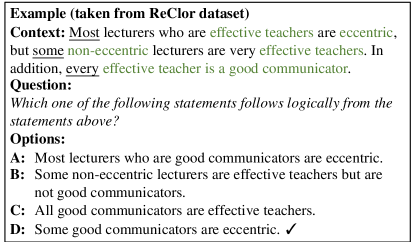
Figure 1: An example from Reclor dataset. The example mainly talks about "effective teachers, non-eccentric, eccentric, good communicator".

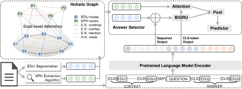
Figure 2: An overview of our proposed holistic graph-based reasoning model.

Logical reasoning MRC tasks are usually to find an appropriate answer, given a set of context and question. Figure 1 shows an example from ReClor dataset Yu et al. (2020) which requires logical reasoning ability to make the correct predictions. As humans, to solve such problems, we usually go through the following steps. Firstly, we divide the context into several fragments and figure out the logical relations between each clause, such as transition, continuity, contrast, etc. Secondly, we extract the important elements in the context, namely, the objects and topics described by the context, and construct the logical graph with these significant elements. Finally, we need to compare the answer statement to the mentioned part in the context and assess its logical fit with the given context.

Most existing methods of logical reasoning MRC focus on either entity-aware or discourse-based information but ignore the hierarchical relations that may have mutual effects Yu et al. (2020); Liu et al. (2020a); Wang et al. (2021); Huang et al. (2021); Ouyang et al. (2021b). Motivated by the observation above, we model logical reasoning chains based on a newly proposed holistic graph network (HGN) that incorporates the information of element discourse units (EDU) Gao et al. (2020); Ouyang et al. (2021a) and key phrases (KPH) extracted from context and answer, with effective edge connection rules to learn both hierarchical features and interactions between different granularity levels.

Our contributions are summarized as follows. (1) We design an extraction algorithm to extract EDU and KPH elements as the critical basic for logical reasoning. (2) We propose a novel holistic graph network (HGN) to deal with context at both discourse and word level with hierarchical interaction mechanism that yields logic-aware representation for reasoning. (3) Experimental results show our model’s strong performance improvements over baselines, across multiple datasets on logical reasoning QA and NLI tasks. The analysis demonstrates that our model has a good generalization and transferability, and achieves higher accuracy with less training data.

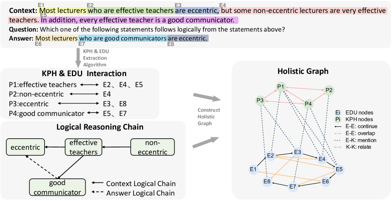
Figure 3: Process of constructing the holistic graph, using KPH-EDU Interaction information and pre-defined rules.

2 Methodology

Logical reasoning MRC tasks aim to find the best answer among several given options based on a piece of context that entails logical relations. Formally, given a natural language context C, a question Q, and four potential answers A=$\{A_{1},A_{2},A_{3},A_{4}\}$. We concatenate them as $\{\textsl{C},\textsl{Q},A_{i}\}$ pairs. To incorporate the principle of human inference into our method, we propose a holistic graph network (HGN) as shown in Figure 2. Our model works as follows. First, we use EDU and KPH extraction algorithm to get necessary KPH nodes ($\{P_{j}\}$) and EDU nodes ($\{E_{j}\}$) from the given pairs. They contain information with different granularity levels and complement each other. Based on the extracted KPH-EDU interaction information and pre-defined rules, we construct the holistic graph. The process of constructing the holistic graph is shown in Figure 3. Then we measure the interaction between $\{E_{j}\}$ and $\{P_{j}\}$ to obtain logic-aware representations for reasoning.

2.1 Logical Chain Construction

Element Discourse Units (EDU)

We use clause-like text spans delimited by logical relations to construct the rhetorical structure of texts. These clause-like discourses can be regarded as element units that reveal the overall logic and emotional tone of the text. For example, conjunctions like "because” indicate a causal relation which means the following discourse is likely to be the conclusion we need to pay attention to. Parenthesis and clauses like "who are effective teachers" in Figure 3 play a complementary role in context. Also, punctuation indicates a pause or an end of a sentence, containing semantic transition and turning point implicitly. We use an open segmentation tool, SEGBOT Li et al. (2018), to identify the element discourse units (EDUs) from the concatenation of context and answer, ignoring the question whose structure is simple. Conjunctions (e.g., "because", "however"), punctuation and the beginning of parenthesis and clauses (e.g., "which", "that") are usually the segment points. They are considered as explicit discourse-level logical relations.

To get the initial embedding of EDUs, we insert an external [CLS] symbol at the start of each discourse, and add a [SEP] symbol at the end of every type of inputs. Then we use RoBERTa to encode the concatenated tokens. The encoded [CLS] token represents the following EDU. Therefore, we get the initial embedding of EDUs.

Key Phrase (KPH)

Key Phrases, including keywords here, play an important role in context. They are usually the object and principle of a context. We use the sliding window to generate $n$-gram word list, filtering according to the Stopword list, POS tagging, the length of the word, and whether it contains any number. The filtering process is based on the following two main criteria:

(1) If the $n$-gram contains a stop word or a number, then delete it.

(2) If the length of word is less than the threshold value $m$, delete it, and if the $n$-gram length is 1, then only the noun, verb, and adjective are retained.

Then, we calculate the TF-IDF features of each $n$-gram, and select the top-$k$ $n$-gram as key phrases. $k$ is a hyper-parameter to control the number of KPHs. We restore the selected tokens and retrieve the original expressions containing the key phrase from the original text. For example, as in Figure 3, "eccentric" is one of the KPHs, while we retrieve the original expression "eccentric" and "non-eccentric" from the original text.

Given the token embedding sequence $K_{i}=\{t_{1},\dots,t_{n}\}$ of a KPH with length $n$, its initial embedding is obtained by

$$P_{i}=\frac{1}{|K_{i}|}\sum_{t_{l}\in K_{i}}t_{l}.$$ (1)

Holistic Graph Construction

Formally, every input sample is a triplet that consists of a context, a question and a candidate answer. EDU and KPH nodes are extracted in the above way. As shown in Figure 3, we construct a holistic graph with two types of nodes: EDU Nodes (in blue) and KPH Nodes (in green). For edge connections, there are four distinct types of edges between pairs of nodes.

$\bullet$ EDU-EDU continue: the two nodes are contextually associated in the context and answer. This type of edge is directional.

$\bullet$ EDU-EDU overlap: the two nodes contain the same KPH. This type of edge is bidirectional.

$\bullet$ EDU-KPH mention: the EDU mentions the KPH. This type of edge is bidirectional.

$\bullet$ KPH-KPH relate: the two nodes are semantically related. We define two types of semantic relations. One is that the two KPHs are retrieved by the same $n$-gram as described above. The other one is that the Cosine similarity between the two KPH nodes is greater than a threshold. This type of edge is bidirectional and can capture the information of word pairs like synonyms and antonyms.

The construction of the graph is based on intuitive rules, which will not introduce extra parameters or increase model complexity. A further parameter comparison is given in Table 4.

2.2 Hierarchical Interaction Mechanism

Considering a specific node in the holistic graph, neighboring nodes in the same type may carry more salient information, thus affecting each other in a direct way. In the process, the neighboring nodes in the different types may also interact with each other. To capture both the node-level and type-level attention, we apply a Hierarchical Interaction Mechanism to the update of the graph network’s representations.

Graph Preliminary

Formally, consider a graph $G=\{V,E\}$, where $V$ and $E$ represent the sets of nodes and edges respectively. $A$ is the adjacency matrix of the graph. $A_{ij}>0$ means there is an edge from the $i$-th node to the $j$-th node. We introduce ${A}^{\prime}=A+I$ to take self-attention into account. In order to avoid changing the original distribution of the feature when multiplying with the adjacency matrix, we normalize ${A}^{\prime}$, set $\tilde{A}=D^{-\frac{1}{2}}{A}^{\prime}D^{-\frac{1}{2}}$ where $D$ is the degree matrix of the graph. $D=diag\{d_{1},d_{2}\dots,d_{n}\}$, $d_{i}$ is the number of edges attached to the $i$-th node.

Now, we calculate the attention score from node ${v}^{\prime}$ to node $v$ in the following steps.

Type Attention Vector

We use $T(\tau)$ to represent all nodes that belong to type $\tau$, and $N(v)$ to represent all neighboring nodes that are adjacent to $v$. $T$ is the set of types. Assume that node $v$ belongs to $T(\tau)$, $h_{\mu}$ is the feature of node $\mu$, $h_{\tau}$ is the feature of type $\tau$ which is computed by

$$h_{\tau}=\sum_{\mu\in T(\tau)}\tilde{A}_{v\mu}Wh_{\mu}.$$ (2)

Using the feature of type and node $v$, we compute the attention score of type $\tau$ as:

$$e_{\tau}=\sigma(\mu_{\tau}^{T}\cdot[Wh_{v}\parallel W_{\tau}h_{\tau}]).$$ (3)

Then, type-level attention weights $\alpha_{\tau}$ is obtained by normalizing the attention scores across all the types $T$ with the softmax function. $\sigma$ is an activate function such as leaky-ReLU.

$$\alpha_{\tau}=\frac{\textup{exp}(\sigma(\mu_{\tau}^{T}\cdot[Wh_{v}\parallel W_{\tau}h_{\tau}]))}{\sum_{{\tau}^{\prime}\in T}\textup{exp}(\sigma(\mu_{{\tau}^{\prime}}^{T}\cdot[Wh_{v}\parallel W_{{\tau}}h_{{\tau}^{\prime}}]))}.$$ (4)

Node Attention Vector

$\alpha_{\tau}$ shows the importance of nodes in type $\tau$ to node $v$. While computing the attention score of node ${v}^{\prime}$ that is adjacent to node $v$, we multiply that by the type attention weights $\alpha_{\tau}$ (assume ${v}^{\prime}$ belongs to type $\tau$). Similarly, node attention weights are obtained by the softmax function across all neighboring nodes.

$$e_{v{v}^{\prime}}=\sigma(\nu^{T}\cdot\alpha_{\tau}[Wh_{v}\parallel Wh_{{v}^{\prime}}]),$$ (5)

$$\alpha_{v{v}^{\prime}}=\frac{\textup{exp}(e_{v{v}^{\prime}})}{\sum_{i\in N(v)}\textup{exp}(e_{vi})},$$ (6)

where $\parallel$ is the concatenation operator and $\alpha_{v{v}^{\prime}}$ is the attention weight from node ${v}^{\prime}$ to $v$.

Update of Node Representation

Let $h_{v}^{(l)}$ be the representation of the node $v$ at the $l$-th layer. Then the layer-wise propagation rule is as follows:

$$h_{v}^{(l+1)}=\sigma(\sum_{{v}^{\prime}\in N(v)}\alpha_{v{v}^{\prime}}Wh_{{v}^{\prime}}^{(l)}).$$ (7)

2.3 Answer Selector

To predict the best answer that fits the logic entailed in the context, we extract the node representations of the last layer of the graph network and feed them into the downstream predictor. For EDU nodes, since the node order implies the occurrence order in the context, we align them with the output of sequence embedding and add to it as a residual part. Therefore, we feed them into a bidirectional gating recurrent unit (BiGRU).

$$\tilde{H}_{E}=\textup{BiGRU}(H_{E}+H_{sent})\in\mathbb{R}^{l\times d},$$ (8)

where $H_{E}=[h_{{v}^{\prime}_{1}},h_{{v}^{\prime}_{2}},\dots,h_{{v}^{\prime}_{l}}]\in\mathbb{R}^{l\times d}$, ${v}^{\prime}_{i}$ belongs to type EDU. $l$ and $d$ are the sequence length and the feature dimension respectively. $H_{sent}$ is the output of sequence embedding.

For KPH nodes, we first expand the embedding of the first [CLS] token to size $1\times d$, denoted as $H_{c}$. Then, we feed the embedding of [CLS] token and features of KPH nodes $H_{K}=[h_{v_{1}},h_{v_{2}},\dots,h_{v_{n}}]\in\mathbb{R}^{n\times d}$ ($v_{i}$ is of KPH type) into an attention layer.

$$\begin{split}\alpha_{i}&=w_{\alpha}^{T}[H_{c}\parallel h_{v_{i}}]+b_{\alpha}\in\mathbb{R}^{1},\\ \tilde{\alpha_{i}}&=\textup{softmax}(\alpha_{i})\in[0,1],\\ \tilde{H}_{c}&=W_{c}\sum_{i}\tilde{\alpha_{i}}h_{v_{i}}+b_{c}\in\mathbb{R}^{1\times d},\end{split}$$ (9)

where $\tilde{\alpha_{i}}$ is the attention weight of node feature $h_{v_{i}}$. $w_{\alpha}$, $b_{\alpha}$, $W_{c}$, and $b_{c}$ are parameters.

The output of BiGRU and the output of attention layer are concatenated and go through a pooling layer, followed by an MLP layer as the predictor. We take a weighted sum of the concatenation as the pooling operation. The predictor is a two-layer MLP with a tanh activation. Specially, coarse-grained and fine-grained features are further fused here to extract more information.

$$\tilde{H}=W_{p}[\tilde{H}_{E}\parallel\tilde{H}_{c}],\quad p=\textup{MLP}(\tilde{H})\in\mathbb{R},$$ (10)

where $W_{p}$ is a learnable parameter, $\parallel$ is the concatenation operator. For each sample, we get $P=[p_{1},p_{2},p_{3},p_{4}]$, $p_{i}$ is the probability of $i$-th answer predicted by model.

The training objective is the cross entropy loss:

$$\mathcal{L}=-\frac{1}{N}\sum_{i}^{N}\log\textup{softmax}(p_{y_{i}}),$$ (11)

where $y_{i}$ is the ground-truth choice of sample $i$. $N$ is the number of samples.

Model	ReClor				LogiQA
	Dev	Test	Test-E	Test-H	Dev	Test
Human ♢	-	63.0	57.1	67.2	-	86.0
RoBERTa${}_{\textsc{base}}$ ♢	55.0	48.5	71.1	30.7	33.3⋆	32.7⋆
HGN${}_{\textsc{RoBERTa(B)}}$	56.3(↑1.3)	51.4(↑2.9)	75.2(↑4.1)	32.7(↑2.0)	39.5(↑6.2)	35.0(↑2.3)
RoBERTa${}_{\textsc{large}}$ ♢	62.6	55.6	75.5	40.0	35.0	35.3
DAGN ♢	65.2	58.2	76.1	44.1	35.5	38.7
DAGN (Aug) ♢	65.8	58.3	75.9	44.5	36.9	39.3
LReasoner${}_{\textsc{RoBERTa}}^{\spadesuit}$	66.2	62.4	81.4	47.5	38.1	40.6
- data augmentation ♠	65.2	58.3	78.6	42.3	-	-
HGN${}_{\textsc{RoBERTa(L)}}$	66.4(↑3.8)	58.7(↑3.1)	77.7(↑2.2)	43.8(↑3.8)	40.1(↑5.1)	39.9(↑4.6)
DeBERTa♠	74.4	68.9	83.4	57.5	44.4	41.5
LReasoner${}_{\textsc{DeBERTa}}^{\spadesuit}$	74.6	71.8	83.4	62.7	45.8	43.3
HGN${}_{\textsc{DeBERTa}}$	76.0(↑1.6)	72.3(↑3.4)	84.5(↑1.1)	62.7(↑5.2)	44.9(↑0.5)	44.2(↑2.7)

Table 1: Experimental results (Accuracy: $\%$) of our model compared with baseline models on ReClor and LogiQA datasets. Test-E and Test-H denote Test-Easy and Test-Hard subclass of the ReClor dataset respectively. The results in bold are the best performance of all models. $\diamondsuit$ indicates that the results are given by Huang et al. (2021), $\spadesuit$ indicates the results are given by Wang et al. (2021), $\star$ means that the results come from our own implementation. roberta(L) and roberta(B) denotes RoBERTa-large and RoBERTa-base, respectively.

% data used	0.1%		1%		10%		100%
	Dev	Test	Dev	Test	Dev	Test	Dev	Test
BERT${}_{\textsc{base}}$	73.2	70.4	77.9	76.8	84.2	83.9	90.8	90.7
RoBERTa${}_{\textsc{large}}$	84.8	82.0	87.6	87.0	89.5	88.8	92.2	91.0
HGN${}_{\textsc{Bert(B)}}$	75.8(↑2.6)	75.4(↑5.0)	81.1(↑3.2)	80.3(↑3.5)	85.4(↑1.2)	83.9(↑0.0)	91.3(↑0.5)	91.0(↑0.3)
HGN${}_{\textsc{RoBERTa(L)}}$	85.4(↑0.6)	83.5(↑1.5)	87.6(↑0.0)	87.3(↑0.3)	90.2(↑0.7)	89.4(↑0.6)	92.3(↑0.1)	91.5(↑0.5)

Table 2: Experimental results (Accuracy: $\%$) on the SNLI dataset. We randomly generate the training dataset with limited size, without changing the size of Dev. and Test set. Bert(B) and RoBERTa(L) denote BERT-base and RoBERTa-large respectively.

Model	Dev				Test
	A1	A2	A3	ANLI	A1	A2	A3	ANLI
RoBERTa${}_{\textsc{large}}$	74.1	50.8	43.9	55.5	73.8	48.9	44.4	53.7
ALUM♠	73.3	53.4	48.2	57.7	72.3	52.1	48.4	57.0
InfoBERT♢	76.4	51.7	48.6	58.3	75.5	51.4	49.8	58.3
HGN${}_{\textsc{RoBERTa(L)}}$	76.7(↑2.6)	69.3(↑18.5)	74.5(↑30.6)	71.3(↑15.8)	79.5(↑5.7)	63.4(↑14.5)	76.3(↑31.9)	68.9(↑15.2)

Table 3: Experimental results (Accuracy: $\%$) on the ANLI dataset. Both ALUM and InfoBERT take RoBERTa-large as the backbone model. $\spadesuit$ means the results from Liu et al. (2020b). $\diamondsuit$ means the results from Wang et al. (2020).

3 Experiment

3.1 Dataset

Our evaluation is based on logical reasoning MRC benchmarks (ReClor Yu et al. (2020) and LogiQA Liu et al. (2020a)) and natural language inference benchmarks (SNLI Bowman et al. (2015) and ANLI Nie et al. (2020)). ReClor contains 6,138 multiple-choice questions modified from standardized tests. LogiQA has more instances (8678 in total) and is derived from expert-written questions for testing human logical reasoning ability Liu et al. (2020a). To assess the generalization of models on NLI tasks, we test our model on the Stanford Natural Language Inference (SNLI) dataset, which contains 570k human annotated sentence pairs. The Adversarial Natural Language Inference (ANLI) is a new large-scale NLI benchmark dataset, where the instances are chosen to be difficult for the state-of-the-art models such as BERT and RoBERTa. It can be used to evaluate the generalization and robustness of the model.

Implementation details and parameter selection are reported in Appendix C for reproduction.

3.2 Main Result

3.2.1 Results on Logical QA

Table 1 presents the detailed results on the development set and the test set of both ReClor and LogiQA datasets. We observe consistent improvements over the baselines. HGN${}_{\textsc{RoBERTa(B)}}$ reaches $51.4\%$ of test accuracy on ReClor, and $35.0\%$ of test accuracy on LogiQA, outperforming other existing models. HGN${}_{\textsc{RoBERTa(L)}}$ reaches $58.7\%$ of test accuracy on ReClor, therein $77.7\%$ on Easy subset and $43.8\%$ on Hard subset, and $39.9\%$ on LogiQA. HGN${}_{\textsc{DeBERTa}}$ achieves $72.3\%$ on the test set of ReClor and $44.2\%$ on LogiQA. If using the same pre-trained language models as the backbones, our proposed model achieves the state-of-the-art results on both ReClor and LogiQA, without extra human annotations. Our model shows great improvement over this task by better utilizing the interaction information , which is ignored by most existing methods.

3.2.2 Results on general NLI tasks

To verify the generality of our model, we conduct experiments on two widely used entailment datasets for NLI: SNLI and ANLI, in which existing models rarely emphasized the modeling of logical relations. Table 2 compares the performances of HGN and baseline models on the SNLI dataset with the same proportion of training data for finetuning. We observe that when given a limited number of training data, our HGN has faster adaptation than baseline models as evidenced by higher performances in low-resource regimes (e.g., $0.1\%$, $1\%$, and $10\%$ of the training data used). HGN also outperforms BERT${}_{\textsc{base}}$ by $0.3\%$ and RoBERTa${}_{\textsc{large}}$ by $0.5\%$ on the full SNLI.

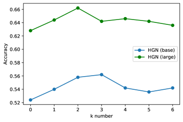
Figure 4: Dev. accuracy on the ReClor dataset as the number of KPH nodes changes.

We assess the model’s robustness against adversarial attacks, using a standard adversarial NLP benchmark: ANLI, as shown in Table 3. A1, A2 and A3 are three rounds with increasing difficulty and data size. ANLI refers to the combination of A1, A2 and A3. HGN${}_{\textsc{RoBERTa(L)}}$ gains a $15.2\%$ points in test accuracy of ANLI over RoBERTa${}_{\textsc{large}}$, creating state-of-the-art results on all rounds. Results show that our model has a comprehensive improvement over baseline models, in aspects of faster adaption, higher accuracy and better robustness.

3.3 More Results

Interpretation of $k$

In this part, we investigate the sensitivity of parameter $k$, which is the number of KPH node. Figure 4 shows the accuracies on the development set of our proposed model with different numbers of KPH nodes, which are extracted according to TF-IDF weights. We observe that $k=2$ or $k=3$ is an appropriate value for our model. This is consistent with our intuition that a paragraph will have 2 to 3 key phrases as its topic. When $k$ is too small or large, the accuracy of the model does not perform well.

Model Complexity

With well-defined construction rules and an appropriate architecture, our model enjoys the advantage of high performance with fewer parameters. We display the statistics of model’s parameters in Table 4. Compared with the baseline model (RoBERTa${}_{\textsc{large}}$), the increase of our model’s parameters is no more than $4.7\%$. Particularly, our model contains fewer parameters and achieves better performance than DAGN.

3.4 Ablation

Model	RoBERTa	DAGN	HGN
Params	356.4M	396.2M	373.4M

Table 4: Statistics of models’ parameters

We conduct a series of ablation studies on Graph Construction, Hierarchical Interaction Mechanism and Answer Selector. Results are shown in Table 5. All models use RoBERTa-base as the backbone.

Holistic Graph Construction

The Holistic Graph in our model contains two types of nodes and four types of edges. We remove the nodes of EDU and KPH respectively and the results show that the removal hurts the performance badly. The accuracies drop to $55.8\%$ and $53.9\%$. Furthermore, we delete one type of edge respectively. The removal of edge type destroys the integrity of the network and may ignore some essential interaction information between EDUs and KPHs, thus causing the drop of the performance.

Hierarchical Interaction Mechanism

Hierarchical Interaction Mechanism helps to capture the information contained in different node types. When we remove the type-level attention, the model is equivalent to a normal Graph Attention Network (GAT), ignoring the heterogeneous information. As a result, the performance drops to $54.8\%$. When we remove both types of attention, the performance drops to $55.7\%$.

Model	Accuracy ($\%$)
HGN${}_{\textsc{base}}$	56.3
Graph Construction
- EDU	55.8 (↓0.5)
- KPH	53.9 (↓2.4)
- edge type: E-E continue	53.0 (↓3.3)
- edge type: E-E overlap	54.0 (↓2.3)
- edge type: E-K mention	54.2 (↓2.1)
Hierarchical Interaction
- type-level attention (i.e. GAT)	54.8 (↓1.5)
- both (i.e. GCN)	55.7 (↓0.6)
Answer Selector
- BiGRU	53.2 (↓3.1)
- Attention layer	55.0 (↓1.3)

Table 5: Ablation results on the dev set of ReClor.

Answer Selector

We make two changes to the answer selector module: (1) deleting the BiGRU, (2) deleting the attention layer. For (1), the output of EDU features concatenates with the output of the attention layer directly and then are fed into the downstream pooling layer. For (2), we ignore the attention between the KPH features and the whole sentence-level features. The resulting accuracies of (1) and (2) drop to $53.2\%$ and $55\%$, which verify that the further fusion of features with different granularity is necessary in our proposed model.

We further analysed the examples that are predicted correctly by our model but not by baselines, and found that the powerful pre-trained language models, such as RoBERTa, would bias for answers with higher similarity to the context or those containing more overlapping words. The model itself does not understand the logical relations, but only compares their common elements for prediction. Instead, our model can not only match synonymic expressions, but also make logical inferences by separating sentences into EDUs and extracting key phrases and establishing logical relations between them. An example is shown in Appendix D.

4 Related Work

4.1 Machine Reading Comprehension

MRC is an AI challenge that requires machines to answer questions based on a given passage, which has aroused great research interests in the last decade Hermann et al. (2015); Rajpurkar et al. (2016, 2018); Lai et al. (2017). Although recent systems have reported human-parity performance on various benchmarks Zhang et al. (2020a); Back et al. (2020); Zhang et al. (2021) such as SQuAD Rajpurkar et al. (2016, 2018) and RACE Lai et al. (2017), whether the machine has necessarily achieved human-level understanding remains controversial Zhang et al. (2020b); Sugawara et al. (2021). Recently, there is increasing interest in improving machines’ logical reasoning ability, which can be categorized into symbolic approaches and neural approaches. Notably, analytical reasoning machine (AMR) Zhong et al. (2021) is a typical symbolic method that injects human prior knowledge to deduce legitimate solutions.

4.2 Logical Reasoning

Neural and symbolic methods have been studied for logical reasoning Garcez et al. (2015); Besold et al. (2017); Chen et al. (2019b); Ren and Leskovec (2020); Huang et al. (2021). Compared with the neural methods for logical reasoning, symbolic approaches like Wang et al. (2021) rely heavily on dataset-related predefined patterns which entails massive manual labor, greatly reducing the generalizability of models. Also, it could introduce propagated errors since the final prediction depends on the intermediately generated functions. Even if one finds the gold programs, executing the program is quite a consuming work as the search space is quite large and not easy to prune. Therefore, we focus on the neural research line in this work, to capture the logic clues from the natural language texts, without the rely on human expertise and extra annotation.

Since the logical reasoning MRC task is a new task that there are only a few latest studies, we broaden the discussion to scope of the related tasks that require reasoning, such as commonsense reasoning Davis and Marcus (2015); Bhagavatula et al. (2020); Talmor et al. (2019); Huang et al. (2019), multi-hop QA Yang et al. (2018) and dialogue reasoning Cui et al. (2020). Similar to our approach of discovering reasoning chains between element discourse and key phrases, Fang et al. (2020) proposes a hierarchical graph network (HGN) that helps to multi-hop QA. Our method instead avoids the incorporation of external knowledge and designs the specific pattern for logical reasoning. Discourse-aware graph network (DAGN) proposed by Huang et al. (2021) also uses discourse relations to help logical reasoning. However, only modeling the relation between sentences will ignore more fine-grained information. Focal Reasoner proposed by Ouyang et al. (2021b), covering global and local knowledge as the basis for logic reasoning, is also an effective approach. In contrast, our work is more heuristic and has a lighter architecture.

Previous approaches commonly consider the entity-level, sentence-level relations, or heavily rely on external knowledge and fail to capture important interaction information, which are obviously not sufficient to solve the problem Qiu et al. (2019); Ding et al. (2019); Chen et al. (2019a). Instead, we take advantages of inter-sentence EDUs and intra-sentence KPHs, to construct hierarchical interactions for reasoning. The fine-grained holistic features are used for measuring the logical fitness of the candidate answers and the given context. As our method enjoys the benefits of modeling reasoning chains from riddled texts, our model can be easily extended to other types of reasoning and inference tasks, especially where the given context has complex discourse structure and logical relations, like DialogQA, multi-hop QA and other more general NLI tasks. We left all the easy empirical verification of our method as future work.

5 Conclusion

This paper presents a novel method to guide the MRC model to better perform logical reasoning tasks. We propose a holistic graph-based system to model hierarchical logical reasoning chains. To our best knowledge, we are the first to deal with context at both discourse level and phrase level as the basis for logical reasoning. To decouple the interaction between the node features and type features, we apply hierarchical interaction mechanism to yield the appropriate representation for reading comprehension. On the logical QA benchmarks (ReClor, LogiQA) and natural language inference benchmarks (SNLI and ANLI), our proposed model has been shown effective by significantly outperforming the strong baselines.

Appendix A KPHs Extraction Algorithm

Algorithm 1 Key Phrases (KPH) Extraction Algorithm

1:Input $C=\{S^{1},S^{2},\dots,S^{I}\}$, $n$-gram length $n$, min word length $m$, number of Key Phrases $k$

2:Set of Key phrases with top-$k$ TF-IDF weights $K=\{g_{1},g_{2},\dots,g_{k}\}$

3:Obtain the TF-IDF dictionary $\mathcal{F}$ = TF-IDF($C$)

4:Generate $n$-gram dictionary $G$ = $n$-gram($C,n$)

5:Filter $n$-gram dictionary $G$, $\tilde{G}$=$\textsc{Filter}(G,m)$

6:Retrieve the original expressions $K$ = Retrieve($C,\mathcal{F},\tilde{G},k$)

7:procedure TF-IDF($C$)

8:     for each sentence in $C$ do

9:         Filter stop-words in the sentence

10:         Calculate the TF-IDF weight for each word

11:     end for

12:     return TF-IDF dictionary $\mathcal{F}$

13:end procedure

14:procedure $n$-gram($C,n$)

15:     for each sentence in $C$ do

16:         Select all gram $g$ with length $n$ in the sentence

17:         Add $g$ to the dictionary $G$

18:     end for

19:     return $n$-gram dictionary $G$

20:end procedure

21:procedure Filter($G,m$)

22:     for each $n$-gram $g$ in $G$ do

23:         if stopwords in $g$ or length$(g)$ is less than $m$ or there is any number in $g$ then

24:              Delete $g$

25:         end if

26:         if length$(g)$ is 1 and POStag($g$) is not noun, verb, or adjective then

27:              Delete $g$

28:         end if

29:     end for

30:     return $n$-gram dictionary $\tilde{G}$

31:end procedure

32:procedure Retrieve($C,\mathcal{F},\tilde{G},k$)

33:     for each $g$ in $\tilde{G}$ do

34:         Calculate the sum of the TF-IDF weights of each word in $g$, add to a dictionary $z=\{g:w(g)\}$

35:     end for

36:     Rank the top-$k$ $n$-gram $g$ by TF-IDF weight sum. Construct key phrases set $K=\{g_{1},g_{2},\dots,g_{k}\}$

37:     if $n$=1 then

38:         for each $g$ in $K$ do

39:              $g_{s}$= STEM($g$)

40:              Retrieve all the original words from $C$ containing $g_{s}$, add to $K$

41:         end for

42:     end if

43:     return Set of Key phrases $K=\{K_{1},K_{2},\dots,K_{k}\}$

44:end procedure

Appendix B Dataset Information

ReClor

The Reading Comprehension dataset requiring logical reasoning (ReClor) is extracted from standardized graduate admission examinations Yu et al. (2020). It contains 6,138 multiple-choice questions modified from standardized tests such as GMAT and LSAT and is randomly split into train/dev/test sets with 4,638/500/1,000 samples respectively. Multiple types of logical reasoning question are included.

LogiQA

LogiQA is sourced from expert-written questions for testing human Logical reasoning. It contains 8,678 QA pairs, covering multiple types of deductive reasoning. It is randomly split into train/dev/test sets with 7,376/651/651 samples respectively.

SNLI

The Stanford Natural Language Inference (SNLI) dataset contains 570k human annotated sentence pairs, in which the premises are drawn from the captions of the Flickr30 corpus and hypotheses are manually annotated. The full dataset is randomly split into 549k/9.8k/9.8k. This is the most widely used entailment dataset for natural language inference. It requires models to take a pair of sentence as input and classify their relation types, i.e., entailment,neutral, or contradiction.

ANLI

The Adversarial Natural Language Inference (ANLI) is a new large-scale NLI benchmark dataset, collected via an iterative, adversarial human-and-model-in-the-loop procedure. Specifically, the instances are chosen to be difficult for the state-of-the-art models such as BERT and RoBERTa. A1, A2 and A3 are the datasets collected in three rounds. A1 and A2 are sampled from Wiki and A3 is from News. It requires models to take a set of context, hyperthesis and reason classify the label (entailment,neutral, or contradiction). A1 has 18,946 in total and is split into 16,946/1,000/1,000. A2 has 47,460 in total and is split into 45,460/1,000/1,000. A3 has 102,859 in total and is split into 100,459/1,200/1,200. ANLI refers to the combination of A1, A2 and A3.

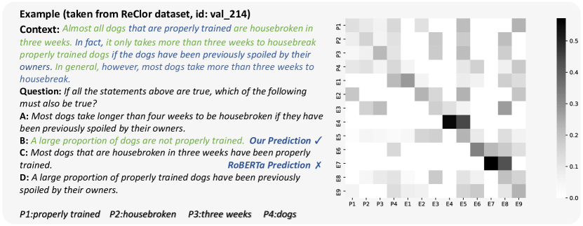
Figure 5: An example showing the logical reasoning capability of our model (Left) and the corresponding attention map (Right). EDUs are shown in different colors alternately, corresponding to E1-E9 in the attention map.

Appendix C Parameter Selection

Our model is implemented based on the Transformers Library Wolf et al. (2020). Adam Kingma and Ba (2015) is used as our optimizer. The best threshold for defining semantic relevance is 0.5. We run 10 epochs for ReClor and LogiQA, 5 epochs for SNLI and ANLI, and select the model that achieves the best result in validation. Our models are trained on one 32G NVIDIA Tesla V100 GPU. The training time is around half an hour for each epoch. The maximum sequence length is 256 for ReClor and SNLI, 384 for LogiQA and 128 for ANLI. The weight decay is 0.01. We set the warm-up proportion during training to 0.1. We provide training configurations used across our experiments in Table 6.

Dataset	PrLM	batchsize	learning rate
ReClor	RoBERTa-base	24	1e-5
	RoBERTa-large	32	8e-6
	DeBERTa-xlarge	8	8e-6
LogiQA	RoBERTa-base	2	4e-6
	RoBERTa-large	2	8e-6
	DeBERTa-xlarge	2	8e-6
SNLI	BERT-base	32	2e-5
	RoBERTa-large	32	2e-5
ANLI	RoBERTa-large	32	2e-05

Table 6: Parameter Selection

Appendix D Case Study

To intuitively show how our model works, we select an example from ReClor as shown in Figure 5, whose answer is predicted correctly by our model but not by baseline models (RoBERTa). The example shows that powerful pre-trained language models such as RoBERTa may be better at dealing with sentence pairs that contain overlap parts or similar words. For example, the wrong answer chosen by RoBERTa is another expression of the first sentence in the given context. The words are basically the same, only the order changes. The model itself does not understand the logical relation between sentences and phrases, but only compares their common elements for prediction, failing in logical reasoning task. In contrast, our model can not only match synonymic expressions, but also make logical inferences by separating sentences into EDUs and extracting key phrases and establishing logical relations between them. The importance of those elements are interpreted by the attention distribution as shown in the right part, which is derived from the last layer of our model.

References

- Back et al. (2020) Seohyun Back, Sai Chetan Chinthakindi, Akhil Kedia, Haejun Lee, and Jaegul Choo. 2020. Neurquri: Neural question requirement inspector for answerability prediction in machine reading comprehension. In 8th International Conference on Learning Representations, ICLR 2020, Addis Ababa, Ethiopia, April 26-30, 2020. OpenReview.net.
- Besold et al. (2017) Tarek R Besold, Artur d’Avila Garcez, Sebastian Bader, Howard Bowman, Pedro Domingos, Pascal Hitzler, Kai-Uwe Kühnberger, Luis C Lamb, Daniel Lowd, Priscila Machado Vieira Lima, et al. 2017. Neural-symbolic learning and reasoning: A survey and interpretation. arXiv preprint arXiv:1711.03902.
- Bhagavatula et al. (2020) Chandra Bhagavatula, Ronan Le Bras, Chaitanya Malaviya, Keisuke Sakaguchi, Ari Holtzman, Hannah Rashkin, Doug Downey, Wen-tau Yih, and Yejin Choi. 2020. Abductive commonsense reasoning. In 8th International Conference on Learning Representations, ICLR 2020, Addis Ababa, Ethiopia, April 26-30, 2020. OpenReview.net.
- Bowman et al. (2015) Samuel R. Bowman, Gabor Angeli, Christopher Potts, and Christopher D. Manning. 2015. A large annotated corpus for learning natural language inference. In Proceedings of the 2015 Conference on Empirical Methods in Natural Language Processing, pages 632–642, Lisbon, Portugal. Association for Computational Linguistics.
- Chen et al. (2019a) Jifan Chen, Shih-ting Lin, and Greg Durrett. 2019a. Multi-hop question answering via reasoning chains. arXiv preprint arXiv:1910.02610.
- Chen et al. (2019b) Xinyun Chen, Chen Liang, Adams Wei Yu, Denny Zhou, Dawn Song, and Quoc V Le. 2019b. Neural symbolic reader: Scalable integration of distributed and symbolic representations for reading comprehension. In International Conference on Learning Representations.
- Choi et al. (2018) Eunsol Choi, He He, Mohit Iyyer, Mark Yatskar, Wen-tau Yih, Yejin Choi, Percy Liang, and Luke Zettlemoyer. 2018. QuAC: Question answering in context. In Proceedings of the 2018 Conference on Empirical Methods in Natural Language Processing, pages 2174–2184, Brussels, Belgium. Association for Computational Linguistics.
- Cui et al. (2020) Leyang Cui, Yu Wu, Shujie Liu, Yue Zhang, and Ming Zhou. 2020. MuTual: A dataset for multi-turn dialogue reasoning. In Proceedings of the 58th Annual Meeting of the Association for Computational Linguistics, pages 1406–1416, Online. Association for Computational Linguistics.
- Davis and Marcus (2015) Ernest Davis and Gary Marcus. 2015. Commonsense reasoning and commonsense knowledge in artificial intelligence. Communications of the ACM, 58(9):92–103.
- Ding et al. (2019) Ming Ding, Chang Zhou, Qibin Chen, Hongxia Yang, and Jie Tang. 2019. Cognitive graph for multi-hop reading comprehension at scale. In Proceedings of the 57th Annual Meeting of the Association for Computational Linguistics, pages 2694–2703, Florence, Italy. Association for Computational Linguistics.
- Fang et al. (2020) Yuwei Fang, Siqi Sun, Zhe Gan, Rohit Pillai, Shuohang Wang, and Jingjing Liu. 2020. Hierarchical graph network for multi-hop question answering. In Proceedings of the 2020 Conference on Empirical Methods in Natural Language Processing (EMNLP), pages 8823–8838, Online. Association for Computational Linguistics.
- Gao et al. (2020) Yifan Gao, Chien-Sheng Wu, Jingjing Li, Shafiq Joty, Steven C.H. Hoi, Caiming Xiong, Irwin King, and Michael Lyu. 2020. Discern: Discourse-aware entailment reasoning network for conversational machine reading. In Proceedings of the 2020 Conference on Empirical Methods in Natural Language Processing (EMNLP), pages 2439–2449, Online. Association for Computational Linguistics.
- Garcez et al. (2015) Artur d’Avila Garcez, Tarek R Besold, Luc De Raedt, Peter Földiak, Pascal Hitzler, Thomas Icard, Kai-Uwe Kühnberger, Luis C Lamb, Risto Miikkulainen, and Daniel L Silver. 2015. Neural-symbolic learning and reasoning: contributions and challenges. In 2015 AAAI Spring Symposium Series.
- Hermann et al. (2015) Karl Moritz Hermann, Tomás Kociský, Edward Grefenstette, Lasse Espeholt, Will Kay, Mustafa Suleyman, and Phil Blunsom. 2015. Teaching machines to read and comprehend. In Advances in Neural Information Processing Systems 28: Annual Conference on Neural Information Processing Systems 2015, December 7-12, 2015, Montreal, Quebec, Canada, pages 1693–1701.
- Huang et al. (2019) Lifu Huang, Ronan Le Bras, Chandra Bhagavatula, and Yejin Choi. 2019. Cosmos QA: Machine reading comprehension with contextual commonsense reasoning. In Proceedings of the 2019 Conference on Empirical Methods in Natural Language Processing and the 9th International Joint Conference on Natural Language Processing (EMNLP-IJCNLP), pages 2391–2401, Hong Kong, China. Association for Computational Linguistics.
- Huang et al. (2021) Yinya Huang, Meng Fang, Yu Cao, Liwei Wang, and Xiaodan Liang. 2021. DAGN: Discourse-aware graph network for logical reasoning. In NAACL.
- Kingma and Ba (2015) Diederik P. Kingma and Jimmy Ba. 2015. Adam: A method for stochastic optimization. In 3rd International Conference on Learning Representations, ICLR 2015, San Diego, CA, USA, May 7-9, 2015, Conference Track Proceedings.
- Lai et al. (2017) Guokun Lai, Qizhe Xie, Hanxiao Liu, Yiming Yang, and Eduard Hovy. 2017. RACE: Large-scale ReAding comprehension dataset from examinations. In Proceedings of the 2017 Conference on Empirical Methods in Natural Language Processing, pages 785–794, Copenhagen, Denmark. Association for Computational Linguistics.
- Li et al. (2018) Jing Li, Aixin Sun, and Shafiq R. Joty. 2018. Segbot: A generic neural text segmentation model with pointer network. In Proceedings of the Twenty-Seventh International Joint Conference on Artificial Intelligence, IJCAI 2018, July 13-19, 2018, Stockholm, Sweden, pages 4166–4172. ijcai.org.
- Liu et al. (2020a) Jian Liu, Leyang Cui, Hanmeng Liu, Dandan Huang, Yile Wang, and Yue Zhang. 2020a. Logiqa: A challenge dataset for machine reading comprehension with logical reasoning. In Proceedings of the Twenty-Ninth International Joint Conference on Artificial Intelligence, IJCAI 2020, pages 3622–3628. ijcai.org.
- Liu et al. (2020b) Xiaodong Liu, Hao Cheng, Pengcheng He, Weizhu Chen, Yu Wang, Hoifung Poon, and Jianfeng Gao. 2020b. Adversarial training for large neural language models. arXiv preprint arXiv:2004.08994.
- Nie et al. (2020) Yixin Nie, Adina Williams, Emily Dinan, Mohit Bansal, Jason Weston, and Douwe Kiela. 2020. Adversarial NLI: A new benchmark for natural language understanding. In Proceedings of the 58th Annual Meeting of the Association for Computational Linguistics. Association for Computational Linguistics.
- Ouyang et al. (2021a) Siru Ouyang, Zhuosheng Zhang, and Hai Zhao. 2021a. Dialogue graph modeling for conversational machine reading. In The Joint Conference of the 59th Annual Meeting of the Association for Computational Linguistics and the 11th International Joint Conference on Natural Language Processing (ACL-IJCNLP 2021).
- Ouyang et al. (2021b) Siru Ouyang, Zhuosheng Zhang, and Hai Zhao. 2021b. Fact-driven logical reasoning. arXiv preprint arXiv:2105.10334.
- Qiu et al. (2019) Lin Qiu, Yunxuan Xiao, Yanru Qu, Hao Zhou, Lei Li, Weinan Zhang, and Yong Yu. 2019. Dynamically fused graph network for multi-hop reasoning. In Proceedings of the 57th Annual Meeting of the Association for Computational Linguistics, pages 6140–6150, Florence, Italy. Association for Computational Linguistics.
- Rajpurkar et al. (2018) Pranav Rajpurkar, Robin Jia, and Percy Liang. 2018. Know what you don’t know: Unanswerable questions for SQuAD. In Proceedings of the 56th Annual Meeting of the Association for Computational Linguistics (Volume 2: Short Papers), pages 784–789, Melbourne, Australia. Association for Computational Linguistics.
- Rajpurkar et al. (2016) Pranav Rajpurkar, Jian Zhang, Konstantin Lopyrev, and Percy Liang. 2016. SQuAD: 100,000+ questions for machine comprehension of text. In Proceedings of the 2016 Conference on Empirical Methods in Natural Language Processing, pages 2383–2392, Austin, Texas. Association for Computational Linguistics.
- Reddy et al. (2019) Siva Reddy, Danqi Chen, and Christopher D. Manning. 2019. CoQA: A conversational question answering challenge. Transactions of the Association for Computational Linguistics, 7:249–266.
- Ren and Leskovec (2020) Hongyu Ren and Jure Leskovec. 2020. Beta embeddings for multi-hop logical reasoning in knowledge graphs. Advances in Neural Information Processing Systems, 33.
- Sugawara et al. (2021) Saku Sugawara, Pontus Stenetorp, and Akiko Aizawa. 2021. Benchmarking machine reading comprehension: A psychological perspective. In Proceedings of the 16th Conference of the European Chapter of the Association for Computational Linguistics: Main Volume, pages 1592–1612.
- Talmor et al. (2019) Alon Talmor, Jonathan Herzig, Nicholas Lourie, and Jonathan Berant. 2019. CommonsenseQA: A question answering challenge targeting commonsense knowledge. In Proceedings of the 2019 Conference of the North American Chapter of the Association for Computational Linguistics: Human Language Technologies, Volume 1 (Long and Short Papers), pages 4149–4158, Minneapolis, Minnesota. Association for Computational Linguistics.
- Wang et al. (2020) Boxin Wang, Shuohang Wang, Yu Cheng, Zhe Gan, Ruoxi Jia, Bo Li, and Jingjing Liu. 2020. Infobert: Improving robustness of language models from an information theoretic perspective. arXiv preprint arXiv:2010.02329.
- Wang et al. (2021) Siyuan Wang, Wanjun Zhong, Duyu Tang, Zhongyu Wei, Zhihao Fan, Daxin Jiang, Ming Zhou, and Nan Duan. 2021. Logic-driven context extension and data augmentation for logical reasoning of text. arXiv preprint arXiv:2105.03659.
- Wolf et al. (2020) Thomas Wolf, Lysandre Debut, Victor Sanh, Julien Chaumond, Clement Delangue, Anthony Moi, Pierric Cistac, Tim Rault, Rémi Louf, Morgan Funtowicz, Joe Davison, Sam Shleifer, Patrick von Platen, Clara Ma, Yacine Jernite, Julien Plu, Canwen Xu, Teven Le Scao, Sylvain Gugger, Mariama Drame, Quentin Lhoest, and Alexander M. Rush. 2020. Transformers: State-of-the-art natural language processing. In Proceedings of the 2020 Conference on Empirical Methods in Natural Language Processing: System Demonstrations, pages 38–45, Online. Association for Computational Linguistics.
- Yang et al. (2018) Zhilin Yang, Peng Qi, Saizheng Zhang, Yoshua Bengio, William Cohen, Ruslan Salakhutdinov, and Christopher D. Manning. 2018. HotpotQA: A dataset for diverse, explainable multi-hop question answering. In Proceedings of the 2018 Conference on Empirical Methods in Natural Language Processing, pages 2369–2380, Brussels, Belgium. Association for Computational Linguistics.
- Yu et al. (2020) Weihao Yu, Zihang Jiang, Yanfei Dong, and Jiashi Feng. 2020. Reclor: A reading comprehension dataset requiring logical reasoning. In 8th International Conference on Learning Representations, ICLR 2020, Addis Ababa, Ethiopia, April 26-30, 2020. OpenReview.net.
- Zhang et al. (2020a) Zhuosheng Zhang, Yuwei Wu, Junru Zhou, Sufeng Duan, Hai Zhao, and Rui Wang. 2020a. Sg-net: Syntax-guided machine reading comprehension. In The Thirty-Fourth AAAI Conference on Artificial Intelligence, AAAI 2020, The Thirty-Second Innovative Applications of Artificial Intelligence Conference, IAAI 2020, The Tenth AAAI Symposium on Educational Advances in Artificial Intelligence, EAAI 2020, New York, NY, USA, February 7-12, 2020, pages 9636–9643. AAAI Press.
- Zhang et al. (2021) Zhuosheng Zhang, Junjie Yang, and Hai Zhao. 2021. Retrospective reader for machine reading comprehension. Proceedings of the AAAI Conference on Artificial Intelligence, 35(16):14506–14514.
- Zhang et al. (2020b) Zhuosheng Zhang, Hai Zhao, and Rui Wang. 2020b. Machine reading comprehension: The role of contextualized language models and beyond. arXiv preprint arXiv:2005.06249.
- Zhong et al. (2021) Wanjun Zhong, Siyuan Wang, Duyu Tang, Zenan Xu, Daya Guo, Jiahai Wang, Jian Yin, Ming Zhou, and Nan Duan. 2021. AR-LSAT: Investigating Analytical Reasoning of Text. arXiv e-prints, page arXiv:2104.06598.