Towards Mitigating Spurious Correlations in the Wild:
A Benchmark & a more Realistic Dataset

Abstract

Deep neural networks often exploit non-predictive features that are spuriously correlated with class labels, leading to poor performance on groups of examples without such features. Despite the growing body of recent works on remedying spurious correlations, the lack of a standardized benchmark hinders reproducible evaluation and comparison of the proposed solutions. To address this, we present SpuCo, a python package with modular implementations of state-of-the-art solutions enabling easy and reproducible evaluation of current methods. Using SpuCo, we demonstrate the limitations of existing datasets and evaluation schemes in validating the learning of predictive features over spurious ones. To overcome these limitations, we propose two new vision datasets: (1) SpuCoMNIST, a synthetic dataset that enables simulating the effect of real world data properties e.g. difficulty of learning spurious feature, as well as noise in the labels and features; (2) SpuCoAnimals, a large-scale dataset curated from ImageNet that captures spurious correlations in the wild much more closely than existing datasets. These contributions highlight the shortcomings of current methods and provide a direction for future research in tackling spurious correlations. SpuCo, containing the benchmark and datasets, can be found at https://github.com/BigML-CS-UCLA/SpuCo, with detailed documentation available at https://spuco.readthedocs.io/en/latest/.

1 Introduction

Spurious correlations pose a formidable challenge in various machine learning tasks, particularly those using deep neural networks. These correlations arise when certain features in the training set are correlated with a given class, but are not predictive of class membership. In such cases, models may learn to exploit these spurious features to predict class labels during training. This leads to poor test performance on examples from the same class that appear without the spurious feature. For example, if the majority of images of dogs appear on a grassy background, the model may incorrectly learn to rely on features of grass to predict membership for class dog. In domains like medicine or public welfare, where it is crucial to ensure a good performance on different groups of examples, spurious correlations can have significant real-world implications.

There has been a growing body of efforts in robust learning against spurious correlations. If group labels indicating whether an example do or do not contains a spurious feature are available at training time, group robust optimization methods Sagawa et al. (2020) or importance weighting Byrd and Lipton (2019) are applied to improve the worst-group performance. In absence of group labels, existing methods aim to first infer the group labels and then apply robust optimization, or importance weighting and resampling on the group-labeled data Creager et al. (2021); Liu et al. (2021); Nam et al. (2022); Sagawa et al. (2020); Yang et al. (2023). Having a group-labeled validation data, semi-supervised learning Nam et al. (2022) or last-layer retraining Kirichenko et al. (2022); Xue et al. (2023) has been shown to be effective in eliminating spurious correlations.

Despite a plethora of methods to mitigate the effect of spurious features while training deep models Creager et al. (2021); Deng et al. (2023); Kirichenko et al. (2022); Liu et al. (2021); Nam et al. (2022); Sagawa et al. (2020); Xue et al. (2023); Yang et al. (2023), this rapidly growing field lacks a standardized benchmark for evaluating and comparing different methods. Moreover, existing spurious benchmark datasets Liu et al. (2015); Sagawa et al. (2020) lack the properties of real-world data, e.g., multiple spurious correlations with various learning difficulty, label and/or feature noise. Therefore, current evaluation schemes do not reflect the effectiveness of existing robust methods in more realistic scenarios, as we confirm experimentally. The lack of a unified implementation and systematic way to evaluate and compare existing methods, not only hinders our understanding of such techniques, but also discourages their usage in practice.

In this paper, we address the above shortcomings by making the following contributions:

• We provide the first open-sourced standardized benchmark, SpuCo, with modular implementations of all current SOTA methods, to enable unified evaluation and ablation of their performance for mitigating spurious correlations in vision datasets.

• Leveraging this benchmark, we show that certain assumptions made in current evaluation pipelines, such as using a pretrained model, do not allow for accurate evaluation of existing robust methods.

• We demonstrate that using a unified evaluation pipeline, Expected Risk Minimization (ERM) with data augmentation is a strong baseline, and Group Balancing can achieve a superior performance to existing SOTA methods. Such results have been missed by prior work.

• To investigate the effectiveness of existing methods against spurious correlations of various learning difficulty, feature and label noise, we design a completely controllable synthetic dataset, SpuCoMNIST. We observe that, existing group-inference methods struggle to find more subtle spurious correlations and group robust optimization is sensitive to even a small fraction of noisy labels.

• We introduce a more realistic dataset, SpuCoAnimals, curated from ImageNet Russakovsky et al. (2015), with four classes and two different spurious correlations. We confirm that current methods methods are not very effective in finding groups and mitigating spurious correlations in real-world datasets.

Our study demonstrates the need for further research to address spurious correlations in the wild.

2 Problem Formulation

Let $\mathcal{D}=\{(\boldsymbol{x}_{i},y_{i})\}_{i=1}^{n}$ be the training data with input features $\boldsymbol{x}_{i}\in\mathbb{R}^{d}$ and labels $y_{i}\in[\mathcal{C}]$ where $\mathcal{C}=\{C_{1},...,C_{l}\}$ are the classes in dataset $\mathcal{D}$. Machine learning models are trained by minimizing an empirical risk function (ERM) using (stochastic) gradient descent. The goal of ERM is to minimize the average error on the entire training data $\mathcal{D}$:

$$\boldsymbol{w}^{*}\in\operatorname*{arg\,min}_{\boldsymbol{w}}\operatorname*{\mathbb{E}}_{(\boldsymbol{x}_{i},y_{i})\in\mathcal{D}}[l(f(\boldsymbol{w},\boldsymbol{x}_{i}),y_{i})],$$ (1)

where $\boldsymbol{w}$ is the model parameter, and $f(\boldsymbol{w},\boldsymbol{x}_{i})$ and $l(f(\boldsymbol{w},\boldsymbol{x}_{i}),y_{i})$ are the output of the network and the value of the loss associated with a training example $(\boldsymbol{x}_{i},y_{i})$, respectively.

Core and Spurious Features Each class is represented by a unique core feature. Let $\mathcal{F}$ be the set of core features where $f_{j}\in\mathcal{F}$ is the core feature for class $C_{j}$. The core feature is indicative of class membership and as such, is present at both training and test time. Additionally, let $\mathcal{S}$ be a set of spurious features that can be shared between classes. These features are present in the data at training time, but are not indicative of class membership and hence, may or may not appear at test time.

For example, in the Waterbirds dataset Sagawa et al. (2020), where the task is to distinguish between waterbirds and landbirds, the core features are the physical characteristics of the birds (e.g. shape of beak, wings) and the spurious features are the backgrounds (e.g. ocean, river, lake, tree, grass).

Groups Examples in the dataset can be partitioned into different groups $g_{f_{j},s_{k}}$, based on the combinations of their core and spurious features $(f_{j},s_{k})$. If a model learns to only rely on a particular spurious feature $s_{k}$ to classify the majority group in class $C_{j}$ at training time, this will result in a poor accuracy on minority groups of class $C_{j}$ that do not contain the spurious feature $s_{k}$ at test time. This is captured by the worst-group error:

Worst-group error We quantify the performance of the model based on its highest test error across groups $\mathcal{G}=\{\cup_{f_{j},s_{k}}~{}g_{f_{j},s_{k}}\}$ in all classes. Formally, worst-group test error is defined as:

$$\text{Err}_{wg}=\max_{g\in\mathcal{G}}\operatorname*{\mathbb{E}}_{(\boldsymbol{x}_{i},y_{i})\in g}\!\![y_{i}\neq\hat{y}(\boldsymbol{w},\boldsymbol{x}_{i})],$$ (2)

where $\hat{y}(\boldsymbol{w},\boldsymbol{x}_{i})$ is the label predicted by the model. In other words, $\text{Err}_{wg}$ measures the highest fraction of examples that are incorrectly classified across all groups.

For example, in the Waterbirds dataset, it is possible that due to the correlation between water backgrounds and waterbirds, the model learns to classify waterbirds using the spurious feature i.e the background rather than the core feature i.e. the characteristics of the birds at training time. However, the water background does not actually determine if a given bird is a waterbird and as such will result in extremely high worst-group error on waterbirds found on land backgrounds.

3 Background

3.1 Existing Methods

Several methods have been proposed to prevent models from exploiting spurious correlations and improve worst group error. If group labels are available, group robust optimization or sampling methods upweight or upsample the minority groups to achieve a similar accuracy on all groups. If group labeled are not available, existing methods first infer groups of the training data and then train the model using robust optimization or sampling techniques with the inferred group labels (c.f. Appendix A).

3.1.1 With Group Labeled Training Data

Sampling Class Balancing (CB) and Group Balancing (GB) sampled every mini-batch to have equal examples from each class and each group, respectively.

GroupDRO (GDRO) leverages group information to sample group-balanced batches of training data, and minimizes the empirical worst-group training loss:

$$\boldsymbol{w}\in\operatorname*{arg\,min}\max_{g\in\mathcal{G}}\operatorname*{\mathbb{E}}_{(\boldsymbol{x}_{i},y_{i})\in g}[l(f(\boldsymbol{w},\boldsymbol{x}_{i}),y_{i})].$$ (3)

GroupDRO solves the above optimization problem by maintaining a weight $q_{g}$ for each group $g$ and weighting the loss of examples in group $g$ by $q_{g}$. Stochastic gradient descent on parameter $\boldsymbol{w}$ is interleaved with gradient ascent on the weights $q_{g}$. GDRO uses a very small tunable learning rate and a large regularizer to achieve a satisfactory performance.

3.1.2 Without Group Labeled Data

In absence of group labels, methods typically infer groups, often using a reference model $f_{ref}$ trained with ERM, and then leverage the inferred groups to train a robust model using sampling or GDRO.

Just Train Twice (JTT) Liu et al. (2021) first trains a reference model $f_{ref}$ using ERM for $T_{r}$ number of epochs. Then, it identifies the minority group as examples that are misclassified by the reference model. JTT then upsamples the misclassified examples $S_{r}$ times and trains another model using ERM on the upsampled dataset. $T_{r}$ and $S_{r}$ are tuned to achieve the optimal performance.

Environment Inference for Invariant Learning (EIIL) EIIL consists of two stages: environment (Group) inference (EI) and invariant learning (IL). In the EI stage, EIIL aims to infer the worst-case groups (environments) using a reference model $f_{ref}$ that has been trained with ERM by optimizing a soft-group assignment $\boldsymbol{q}$ to maximize the following objective:

$$C^{EI}(f_{ref},\boldsymbol{q})=\|\nabla_{\bar{\boldsymbol{w}}}\tilde{R}^{e}(\bar{\boldsymbol{w}}\cdot f_{ref},\boldsymbol{q})\|.\quad\text{s.t.}\quad\tilde{R}^{e}(f_{ref},\boldsymbol{q})=\frac{1}{N}\sum_{i}q_{i}(e)l(f_{ref}(\boldsymbol{x}_{i}),y_{i}).$$ (4)

where $\bar{\boldsymbol{w}}$ is the all-ones vector. Intuitively, the group assignment $\boldsymbol{q}$ is optimized to find examples that are most sensitive to small changes in the reference model $f_{ref}$’s outputs. In the IL stage, EIIL uses GroupDRO with the inferred groups to train a robust model.

Separate Early and Re-sample (Spare) Spare Yang et al. (2023) proved that in the presence of strong spurious correlations, the outputs of a neural network trained with ERM are mainly determined by the spurious features, early-in-training. Thus, it infers groups by clustering the reference model $f_{ref}$’s output on each class, where $f_{ref}$ is trained for a few $T_{r}$ epochs. The inferred groups (clusters) are then used to train a model with importance sampling based on the cluster sizes, to balance the groups. Number of clusters and $T_{r}$ are tuned to achieve best performance.

3.1.3 Using the Group-Labeled Validation Set

Spread Spurious Attributes (SSA) SSA (Nam et al., 2022) leverages the group labeled validation data to train a group label predictor in a semi-supervised manner. Given a training example $\boldsymbol{x}_{i}$, let $g$ denotes its (unknown) group label, $\hat{p}(\cdot|\boldsymbol{x}_{i})$ denotes the model’s predicted group label distribution and $\hat{g}\coloneqq\arg\max_{g\in\mathcal{A}}\hat{p}(g|\boldsymbol{x}_{i})$ denotes the predicted group label. SSA minimizes the following loss function:

$$\mathcal{L}=\hat{\mathbbm{E}}_{\text{group labeled}}[\text{CE}(\hat{p}(\cdot|\boldsymbol{x}),g)]+\hat{\mathbbm{E}}_{\text{group-unlabeled}}[\mathbbm{1}_{\max_{g\in\mathcal{A}}\hat{p}(g|\boldsymbol{x})\geq\tau}\text{CE}(\hat{p}(\cdot|\boldsymbol{x}),\hat{g})],$$

where CE is the cross entropy loss. Effectively, in addition to fitting the available group labels (validation set), SSA uses the group unlabeled examples with confident predictions (larger than a threshold $\tau$) as additional group labeled data. Moreover, SSA partitions the group unlabeled data into multiple splits and trains a group label predictor for each left out split by using the other splits as the group unlabeled training data. The threshold $\tau$ and the number of splits are both tuned to achieve optimal performance.

Deep Feature Reweighting (DFR) DFR Kirichenko et al. (2022) argues that a model trained with ERM captures both core and spurious features in its last hidden layer, even though it may exhibit spurious correlations in its predictions. Motivated by this, DFR retrains the last linear layer of the model on a group-balanced validation data, while keeping earlier layers frozen. This enables the model to adjust the weights assigned to the features in the penultimate layer. DFR trains multiple linear models with tunable $\ell_{1}$ regularization on randomly sampled group-balanced validation data and averages their weights.

Dispel Xue et al. (2023) obtains a superior performance when a small group-balanced validation data is available, by leveraging the richer features found in a larger data without group labels. Similar to DFR, it retrains the last layer of a model trained with ERM. For each embedding $\bm{z}$ from the group-unlabeled data, a corresponding embedding $\bm{z}^{\prime}$ is randomly selected from the group-balanced data in the same class as $\bm{z}$. A new mixed embedding is then created using $s\bm{z}^{\prime}+(1-s)\bm{z}$, where $s\in[0,1]$. Dispel retrains the last linear layer on the mixed embeddings. Similar to DFR, it also uses $\ell_{1}$ regularization and an ensemble of multiple linear models trained on randomly sampled group-balanced data.

3.2 Existing Vision Datasets

Existing spurious benchmark datasets such as Waterbirds Liu et al. (2015), and CelebA Sagawa et al. (2020) are often too simplistic and do not capture properties of real-world data. In particular, they are mainly restricted to binary classification in presence of one easy-to-learn spurious feature. As a results, nearly all the aforementioned methods achieve a similar worst-group accuracy on existing spurious vision datasets. Importantly, such datasets often require a pretrained network to be able to achieve a satisfactory performance, as we will confirm next. However, a pretrained model may not be available in many scenarios. Besides, this prevents accurate evaluation of the performance of the robust methods, as it is not clear if the improved worst-group accuracy is contributed to reweighting the core feature already learned by the pretrained model, or the proposed robust learning method. While a few other datasets has been recently proposed, namely Spawrious Lynch et al. (2023) and Whac-a-mole Li et al. (2023), they are synthetically generated and only contain one easy-to-learn spurious feature. This does not reflect the effectiveness of robust methods on more realistic datasets, as is evident by their high worst-group performance Li et al. (2023); Lynch et al. (2023). In contrast, real-world datasets may contain multiple spurious features with various levels of learning difficulties, as well as feature and label noise. As we will show next, learning difficulties of the spurious and core features, and other factors such as label noise, plays a significant role in the success of existing robust methods. In Sec. 6 we introduce a more realistic dataset, which enables better evaluation of robust methods for eliminating spurious correlations in the wild.

4 Reproducing Results on Waterbirds

Table 1: Worst-group and average accuracy ($\%$) of training with state-of-the-art algorithms on Waterbirds. CB, GB indicate balancing classes and groups, respectively. * indicates using data augmentation, and $\diamond$ indicates that early stopping is not used. For all the other methods, we apply early stopping based on the worst-group validation accuracy.

	Group	Train	Reported (pretrained)		SpuCo (pretrained)		SpuCo (from-scratch)
	Info	Cost	Worst-group	Average	Worst-group	Average	Worst-group	Average
ERM⋄	$\times$	1x	$60.0$	$97.3$	$65.7_{\pm 0.0}$	$97.3_{\pm 0.0}$	$12.8_{\pm 4.6}$	$88.5_{\pm 0.1}$
ERM∗⋄	$\times$	1x	$74.9_{\pm 2.4}$	$98.1_{\pm 0.1}$	$74.9_{\pm 1.7}$	$98.1_{\pm 0.1}$	$10.3_{\pm 2.1}$	$89.3_{\pm 0.2}$
ERM∗	$\times$	1x	-	-	$80.1_{\pm 0.7}$	$97.8_{\pm 0.3}$	$23.5_{\pm 5.0}$	$82.2_{\pm 6.4}$
CB∗	$\times$	1x	-	-	$71.7_{\pm 1.6}$	$97.1_{\pm 0.1}$	$28.4_{\pm 4.7}$	$77.4_{\pm 7.8}$
EIIL	$\times$	1x	$78.7$	$96.9$	$83.5_{\pm 2.8}$	$94.2_{\pm 1.3}$	$45.5_{\pm 3.2}$	$51.1_{\pm 3.2}$
JTT	$\times$	5x-6x	$86.7$	$93.3$	$83.1_{\pm 3.5}$	$90.6_{\pm 0.3}$	$15.7_{\pm 1.6}$	$85.7_{\pm 0.4}$
Spare	$\times$	1x	${89.8}_{\pm 0.6}$	$94.2_{\pm 1.6}$	$91.6_{\pm 0.8}$	$96.2_{\pm 0.6}$	$50.6_{\pm 1.3}$	$59.5_{\pm 4.9}$
SSA	validation	1.5x-5x	$89.0_{\pm 0.6}$	$92.2_{\pm 0.9}$	$85.1_{\pm 1.3}$	$96.7_{\pm 1.6}$	$47.8_{\pm 1.7}$	$62.1_{\pm 8.2}$
$\text{DFR}^{Val}_{Tr}$	validation	1x	$92.9_{\pm 0.2}$	$94.2_{\pm 0.4}$	$90.6_{\pm 0.4}$	$93.4_{\pm 0.2}$	$50.8_{\pm 1.8}$	$63.8_{\pm 1.1}$
Dispel	validation	1x	$92.8_{\pm 0.6}$	$94.2_{\pm 0.2}$	$92.7_{\pm 0.4}$	$94.4_{\pm 0.6}$	$51.9_{\pm 1.2}$	$65.2_{\pm 1.6}$
GB	training	1x	-	-	$88.1_{\pm 0.6}$	$95.5_{\pm 0.4}$	$50.6_{\pm 1.1}$	$64.3_{\pm 2.1}$
GB∗	training	1x	-	-	$87.5_{\pm 0.9}$	$93.4_{\pm 2.5}$	$50.8_{\pm 1.9}$	$61.7_{\pm 7.7}$
GDRO	training	1x	$86.0$	$93.2$	$85.7_{\pm 0.8}$	$94.3_{\pm 1.0}$	$50.7_{\pm 0.7}$	$65.1_{\pm 1.2}$

We provide a spurious benchmark package SpuCo, containing the implementations of all the methods discussed in Sec. 3. Table 1 compares our reproduced results averaged over 3 runs with the reported numbers All the hyperparameters specified in Sec. 3 are tuned via the group-labeled validation set. Details about the hyperparameters can be found in the Appendix B. Our results closely align with the reported numbers, providing validation for our implementation. We make the following observations:

• ERM with data augmentation can achieve a competitive worst-group performance with some group inference methods. The poor performance of ERM reported in prior work seems to be contributed to not using data augmentation and early stopping.

• GB can outperform GDRO. This observation has been missed by prior studies.

• Having access to a pretrained model and a group-labeled validation data, retraining the last-layer is an effective method to eliminate the spurious correlation, and can outperform GB and DGRO.

• Finding majority groups containing the spurious feature early in training and downsampling them (Spare) can be more promising than finding and upsampling the minorities.

• Importantly, using a pretrained network seems to be essential for all the methods to be able to learn from Waterbirds. This prevents an accurate evaluation, as we will discuss next.

Use of pretrained models. All existing methods initialize their model using weights pretrained on ImageNet. This does not allow accurate evaluation of the methods, as it is not clear if a core feature is learned by the model during robust training, or has been learned in the pretrained weights. In Table 1, we also present results for training from random initialization. Remarkably, in this scenario, none of the methods exhibit a notable improvement over random guessing. Notably, even GB, where groups are exactly balanced, only achieves random chance performance. This is mainly contributed to the limited sample size and the inherent difficulty of learning the core features, i.e., waterbirds vs. landbirds. In Sec. 6, we propose a more realistic dataset, where significant improvements can be anticipated by addressing the spurious correlations, without the need for a pretrained network.

5 SpuCoMNIST: Effect of Spurious Feature & Noise on Robust Methods

First, we do an extensive empirical study on how spurious features are learned and investigate various factors that can affect the performance of current methods on real-world datasets. To do so, we introduce a new synthetic dataset, SpuCoMNIST   based of the colored digit recognition dataset CMNIST Arjovsky et al. (2019). The task is digit recognition on MNIST digits but colored backgrounds are added to the MNIST digits as the spurious features. In addition to the number of classes, and group sizes, SpuCoMNIST allows for controlling the magnitude and variance of the spurious features, as well as label noise and noise on the core feature. Such factors are not captured by existing synthetic datasets such as CMNIST and Waterbirds. In Sec. 6, we confirm the importance of these factors on the performance of robust methods on real-world datasets.

Experiment Setup We instantiate a 5 class version of SpuCoMNIST  with consecutive digits i.e are grouped into a single class. The set of spurious features is 5 colored backgrounds. Each class is spuriously correlated with a particular colored background and the size of each majority group is $99.5\%$ of the class. We use LeNet as our model and SGD as our optimizer (c.f. Appendix C for details).

Table 2: Existing methods against label noises and feature noises. To simplify the setting, we only consider the scenario in which the samples have large magnitude of spurious features. For label and feature noise experiments, the spurious feature has no variance and large magnitude.

	ERM		GDRO		JTT		Group Balancing
Spurious Magnitude	Worst-group	Average	Worst-group	Average	Worst-group	Average	Worst-group	Average
Large	$0.0_{\pm 0.0}$	$99.5_{\pm 0.0}$	$74.8_{\pm 2.8}$	$98.8_{\pm 0.3}$	$76.4_{\pm 6.1}$	$97.6_{\pm 1.3}$	$76.8_{\pm 2.8}$	$97.3_{\pm 0.3}$
Medium	$66.0_{\pm 5.0}$	$89.9_{\pm 7.0}$	$90.4_{\pm 1.9}$	$96.1_{\pm 0.4}$	$65.0_{\pm 18.4}$	$96.8_{\pm 0.1}$	$92.9_{\pm 0.1}$	$96.5_{\pm 0.6}$
Small	$97.0_{\pm 0.5}$	$98.7_{\pm 0.2}$	$96.6{\pm 0.4}$	$98.7_{\pm 0.3}$	$94.8_{\pm 1.0}$	$98.4_{\pm 0.4}$	$95.8_{\pm 0.6}$	$98.2_{\pm 0.4}$
Spurious Variance	Worst-group	Average	Worst-group	Average	Worst-group	Average	Worst-group	Average
Low	$44.6_{\pm 4.1}$	$99.8_{\pm 0.1}$	$84.3_{\pm 1.7}$	$98.3_{\pm 1.2}$	$82.7_{\pm 7.8}$	$97.4_{\pm 1.1}$	$86.3_{\pm 2.2}$	$97.3_{\pm 1.2}$
Medium	$44.3_{\pm 4.0}$	$99.8_{\pm 0.1}$	$91.4_{\pm 0.4}$	$96.9_{\pm 0.4}$	$75.1_{\pm 24.2}$	$97.7_{\pm 1.5}$	$92.9_{\pm 0.1}$	$96.5_{\pm 0.6}$
High	$86.4_{\pm 0.4}$	$95.1_{\pm 1.2}$	$92.3_{\pm 0.6}$	$97.2_{\pm 0.1}$	$32.5_{\pm 43.7}$	$96.2_{\pm 0.6}$	$92.2_{\pm 0.5}$	$96.2_{\pm 0.6}$
Label Noise	Worst-group	Average	Worst-group	Average	Worst-group	Average	Worst-group	Average
$0\%$	$0.0_{\pm 0.0}$	$99.5_{\pm 0.0}$	$74.8_{\pm 2.8}$	$98.0_{\pm 0.3}$	$76.4_{\pm 6.1}$	$97.6_{\pm 1.3}$	$76.8_{\pm 2.8}$	$97.3_{\pm 0.3}$
$0.01\%$	$0.0_{\pm 0.0}$	$99.5_{\pm 0.0}$	$70.3_{\pm 2.3}$	$96.9_{\pm 0.5}$	$69.7_{\pm 1.3}$	$97.3_{\pm 0.2}$	$71.7_{\pm 2.7}$	$96.8_{\pm 0.4}$
$0.1\%$	$0.0_{\pm 0.0}$	$99.5_{\pm}{0.0}$	$56.9_{\pm 5.6}$	$96.6_{\pm 1.1}$	$64.4_{\pm 1.9}$	$95.2_{\pm 1.3}$	$64.2_{\pm 1.1}$	$95.1_{\pm 1.4}$
Feature Noise	Worst-group	Average	Worst-group	Average	Worst-group	Average	Worst-group	Average
$0\%$	$0.0_{\pm 0.0}$	$99.5_{\pm 0.0}$	$74.8_{\pm 2.8}$	$98.0_{\pm 0.3}$	$76.4_{\pm 6.1}$	$97.6_{\pm 1.3}$	$76.8_{\pm 2.8}$	$97.3_{\pm 0.3}$
$10\%$	$0.0_{\pm 0.0}$	$99.5_{\pm 0.0}$	$71.4_{\pm 0.4}$	$98.0_{\pm 0.4}$	$75.1_{\pm 3.4}$	$95.2_{\pm 1.3}$	$81.9_{\pm 1.1}$	$97.6_{\pm 0.3}$
$20\%$	$0.0_{\pm 0.0}$	$99.5_{\pm 0.0}$	$67.2_{\pm 3.1}$	$98.1_{\pm 0.2}$	$69.0_{\pm 8.3}$	$96.0_{\pm 0.3}$	$78.0_{\pm 6.6}$	$97.1_{\pm 0.4}$

Effect of Magnitude and Variance of Spurious Features We start by studying the effect of learning spurious features of different difficulties, determined here by their magnitude and variance Yang et al. (2023). In SpuCoMNIST, the magnitude of the spurious feature is varied by changing the size of the colored background patch. The variance of the spurious feature is controlled by keeping the number of pixels of the colored background patch constant, but allowing them to be selected from a larger (smaller) range to allow for more (less) variation in spurious backgrounds. Fig. 1 shows examples of SpuCoMNIST digits with three magnitude levels (large, medium and small) and three variance levels (low, medium, high). Spurious features with larger magnitude or lower variance are easier to learn.

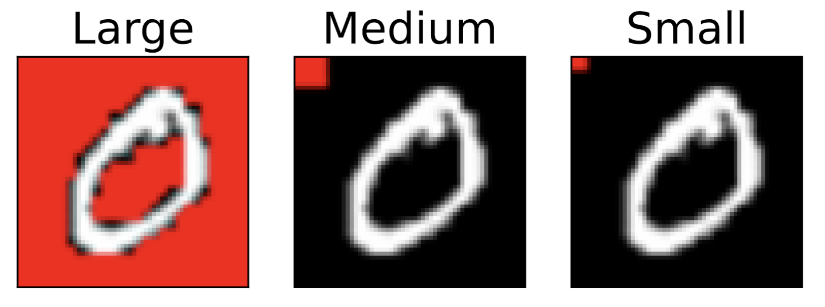
(a) Magnitude

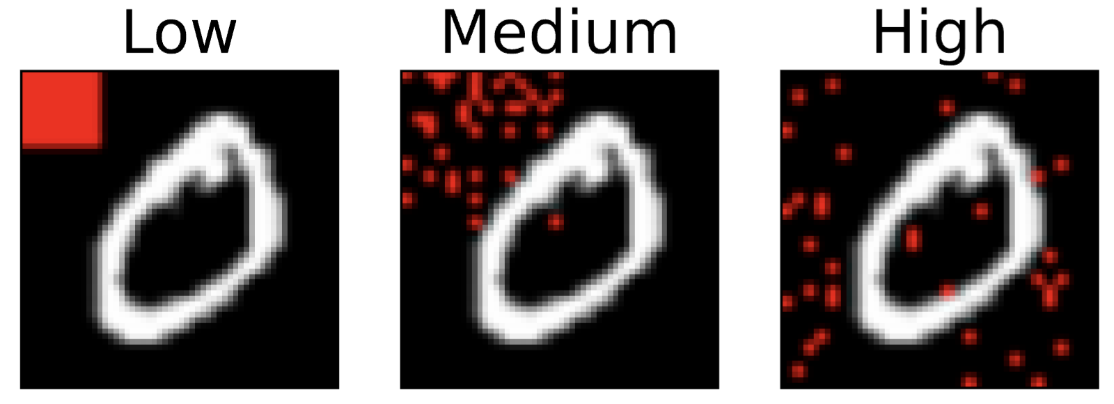
(b) Variance

(c) Feature Noise

Figure 1: Examples of images in SpuCoMNIST.

Table 2 summarizes the results (more comparison can be found in Appendix D). We observe that spurious features with larger magnitude or lower variance have a more drastic impact on the performance of the networks trained with ERM. In particular, large magnitude results in 0% worst-group accuracy for ERM. Similarly, low variance of the spurious features results in a worst-group accuracy that is a half of what ERM obtains under a high variance. This is because learning a spurious feature with a large magnitude and/or small variance is easier. Hence, the network relies more on such spurious features and remains invariant to the core features of the majority groups. At the same time, varying the magnitude and variance of the spurious feature does not have a significant effect on the average accuracy of the network. For GDRO and GB, a similar trend can be observed. However, under large-to-medium magnitude or low-to-high variance of the spurious feature, JTT suffers from poor and extremely unstable worst group accuracy. This is because JTT finds the minority group as misclassified examples at a given epoch. When learning the spurious feature is more difficult, the majority group is not learned reliably by any particular epoch and hence the minority group is more difficult to distinguish based on misclassification.

Effect of Label Noise and Noise on Core Features Next, we study the effect of label noise and noise on the core features on the performance of ERM and existing robust methods. To disentangle the effects of spurious feature magnitude and variance, the spurious feature is set to have no variance and large magnitude (easiest-to-learn spurious feature). Fig. 1 shows an example of noisy digit 0.

For label noise, perhaps surprisingly, the worst-group performance of JTT is less affected than GDRO. As mislabeled examples originally belong to the majority group w.h.p, they end up in the minority group of the other class. As a results, GDRO increase the minority group weight and the model tries to learn the core feature for the wrong class. This, in turn, results in a larger weight on the majority group of the original class, yielding poor final worst-group performance (c.f. Appendix C). On the other hand, JTT includes the mislabeled majority examples in its inferred minority group and heavily upsamples them. This results in the network overfitting the individual misclassified examples, not an entire group. Hence, label noise does not affect JTT’s worst-group performance as much as GDRO. Notably, for both GDRO and JTT, the average accuracy is more affected than ERM. In contrast, GB is more robust to noisy labels.

For noise on the core feature, we see that feature noise makes it more difficult to learn the core features of the minorities and harms the worst-group performance of GDRO. Interestingly, as majorities can be correctly classified by the spurious feature, feature noise on the core feature does not harm the average performance of ERM and GDRO. However, feature noise makes it more difficult to infer the groups based on misclassification. This harms both the average and worst-group accuracy of JTT.

The above observations highlight the vulnerability of existing methods to factors that are likely to occur in real-world scenarios but are not adequately captured by existing datasets. We believe that SpuCoMNIST, which allows for the controlled introduction of these factors, can let researchers gain deeper insights into the challenges posed by real-world scenarios and develop more robust methods.

Next, we introduce a more realistic vision dataset, namely SpuCoAnimals   and confirm that validity of the above conclusions in real-world datasets.

6 SpuCoAnimals: Large Scale Realistic Image Dataset

Next, we introduce SpuCoAnimals, a large scale vision dataset curated from ImageNet with two realistic spurious correlations Russakovsky et al. (2015). SpuCoAnimals has 4 classes: landbirds, waterbirds, small dog breeds and big dog breeds. Waterbirds and Landbirds are spuriously correlated with water and, land backgrounds, respectively. Small dogs and big dogs are spuriously correlated with indoor and outdoor backgrounds, respectively.

Dataset Construction The images for this dataset are curated from fine-grained classes of ImageNet Russakovsky et al. (2015) that correspond to the coarse-grained classes of SpuCoAnimals. The group labels are obtained using CLIP, which is a large language-image model pretrained on 400 million image-captions pairs crawled from the internet Radford et al. (2021). CLIP allows zero-shot image classification, by matching the representation of an image to the most similar caption representation, among the available ones. To construct the caption set, we use the following template: {keyword} background . In classes waterbirds and landbirds, for land backgrounds we used keywords: grass, forest, tree, and for water background we used keywords: lake, river, sea, and ocean. For classes small dogs and big dogs, for indoor background, we used keywords: bed, couch and floor. For outdoor backgrounds we used keywords: grass, park and road. We run zero-shot classification on birds and dogs separately with the respective caption sets. The training set has 10500 examples per class with a 20:1 ratio between majority and minority group for each class. The validation set has 525 examples for each class with the same ratio of majority to minority groups. The test set is group-balanced and has 500 examples per group. Details about the prompts, confidence thresholds and underlying ImageNet classes used in constructing this dataset appear in Appendix E. Fig. 2 shows examples of images for each of the 8 groups in SpuCoAnimals.

SpuCoAnimals vs. Existing Datasets SpuCoAnimals is a more realistic dataset curated from ImageNet and hence contains natural variation in spurious features, as discussed in Sec. 5. Besides, due to its larger size (an order of magnitude larger than Waterbirds Sagawa et al. (2020)) and the more realistic core and spurious features, it does not require a pretrained model, and can be used to train from random initialization. Finally, SpuCoAnimals deviate from traditional binary classification with one easy-to-learn spurious feature in Waterbirds Sagawa et al. (2020) and CelebA Liu et al. (2015), by having four classes with two spurious correlations. This enables better evaluation of the performance of the robust methods in the wild.

6.1 Validating the Spurious Correlation in SpuCoAnimals

First, we confirm that the two spurious correlations are learned by ERM, and GradCam visualizations.

ERM Table 3 list the accuracy of ERM on each of the 8 groups in the datasets. The poor worst-group accuracy of ERM confirms that the spurious features are learned for the majority groups. In particular, the minority groups in the two dog classes (big dogs indoor and small dogs outdoor) have lower worst-group accuracy (8.33%, 10.20%) than the minority groups in the two bird classes (waterbirds on land and landbirds on water with 12.47%, 33.2% worst-group accuracy, respectively). This is contributed to the difference in the magnitude and variance of the spurious vs core features in the two classes (c.f. Sec. 5). Hence, the various core and spurious features are learned at different times and to different extents.

GradCam We further leverage GradCam to validate that the spurious features are used by the model to make predictions on the majority groups. GradCAM visualization in Fig. 2 show that most of the attention (indicated by warmer colors) is focused on the background (spurious feature) rather than the bird / dog (core feature). This confirms that spurious features are leveraged to predict the class.

Table 3: ERM Group-Wise Test Accuracy

Group	Size	Accuracy
Landbirds on Land	10000	$78.8_{\pm 4.0}$
Landbirds on Water	500	$33.2_{\pm 10.2}$
Waterbirds on Land	500	$12.5_{\pm 10.5}$
Waterbirds on Water	10000	$86.3_{\pm 2.7}$
Small Dogs Indoors	10000	$89.9_{\pm 1.2}$
Small Dogs Outdoors	500	$8.3_{\pm 1.3}$
Big Dog Indoors	500	$10.2_{\pm 2.3}$
Big Dog Outdoors	10000	$78.9_{\pm 8.2}$

6.2 Evaluation of Existing Robust Methods

Next, we compares the performance of existing methods when training ResNet-18 from random initialization on the more realistic SpuCoAnimals dataset. Table 1 shows that existing robust methods struggle to truly resolve the spurious correlation on SpuCoAnimals evidenced in Table 4, and often achieve a poor worst-group and average accuracy. In particular, we make the following observations.

With Group Labeled Training Data Methods that use group labeled training data such as GDRO and GB obtain the highest worst-group accuracy. Notably, GB outperforms GDRO. This is consistent with our observations on Waterbirds Sagawa et al. (2020) and SpuCoMNIST datasets in Tables 1 and 2, respectively. When groups are significantly imbalanced, GB consistently outperforms GDRO across all datasets. This is because the group balanced batches (used by both GB and GDRO) ensures that minority group examples are trained on several more times than majority groups, leading to the model having low training loss on minority groups. This, in turn, causes GDRO to upweight the loss of majority groups (because GDRO upweights high loss groups) leading to learning the spurious features. However, GB doesn’t reweight the group loss and thus can outperform GDRO. Moreover, GB achieves the highest performance across all methods when used with data augmentation.

Without Group Labels Next, we see that the different learning dynamics of core and spurious features in the four classes makes it much more difficult for the group inference methods to find the minority groups. As confirmed by Table 4, group inference methods such as EIIL and JTT struggle to find the minority groups, and obtain very poor worst-group performances. Consistent with our observations in Sec. 5, finding the majority groups early in training and alleviating their effect, as is done by Spare, seems to be more promising than finding minorities. However, group inference seems to be much more challenging in more realistic scenarios, and all the group inference methods are edged out by methods that leverage the group labels.

Using the Group-Labeled Validation Set Finally, we see that DFR and Dispel that leverage a group-labeled validation data outperform group inference methods and are able to match GDRO, but are outperformed by GB.

Our SpuCoAnimals dataset confirms that mitigating spurious correlations from real-world dataset is still an open problem, and more efforts are required to develop more principled techniques to identify and boost the worst-group performance on the minority groups.

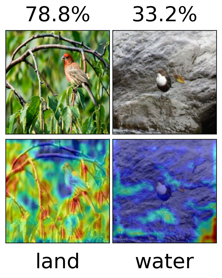
(a) Land Bird

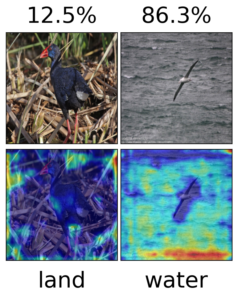
(b) Water Bird

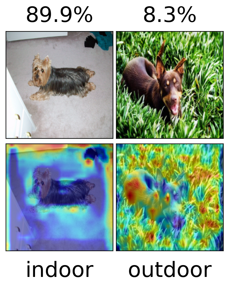
(c) Small Dog

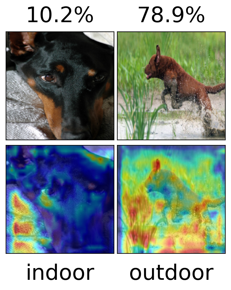
(d) Big Dog

Figure 2: GradCAM Selvaraju et al. (2017) Visualizations reveal that a model trained with ERM primarily focuses on the spurious feature (background) of images within each group, while failing to learn the core feature.

Method	ERM∗	JTT	EIIL	Spare	GDRO	GB	GB∗	DFR	Dispel
Group Label	✗	✗	✗	✗	✓	✓	✓	✓	✓
Worst-group	$9.5_{\pm 4.7}$	$11.8_{\pm 2.6}$	$12.9_{\pm 1.8}$	$31.2_{\pm 2.9}$	$36.7_{\pm 0.6}$	$41.1_{\pm 2.7}$	$49.1_{\pm 2.3}$	$42.6_{\pm 7.8}$	$44.2_{\pm 1.4}$
Average	$84.6_{\pm 3.1}$	$60.6_{\pm 0.8}$	$69.4_{\pm 9.0}$	$46.8_{\pm 2.9}$	$50.7_{\pm 4.2}$	$49.9_{\pm 1.4}$	$59.87_{\pm 6.34}$	$69.0_{\pm 1.5}$	$65.75_{\pm 1.1}$

Table 4: Worst-group and average accuracy ($\%$) of training with state-of-the-art algorithms on SpuCoAnimals. CB, GB indicate balancing classes and groups, respectively.

7 Conclusion

We provide the first open-sourced standardized benchmark, SpuCo, which offers a convenient and rigorous way to benchmark existing and future solutions designed to tackle spurious correlations. Our extensive evaluations confirmed that: (1) perhaps surprisingly, ERM with augmentations is a strong baseline and group balancing can achieve state-of-the-art performance; (2) finding the majority groups early in training seems to be more promising than other group inference techniques; (3) last-layer retraining is an effective way of eliminating spurious correlations, in presence of a group-labeled validation data. Furthermore, we introduced a synthetic and a real-world dataset. Our synthetic datasets, SpuCoMNIST, provides controllable parameters that enable better understanding and debugging of the success and failure modes of current and future methods. Our real-world dataset, SpuCoAnimals, provides a challenging large-scale dataset that demonstrates the need for further research to be able to address spurious correlations in real-world datasets.

Limitation and Broader Impact While our benchmark includes realistic vision datasets and exhaustive evaluations of the existing methods on vision benchmark datasets, we do not propose natural language datasets nor include evaluations of the existing methods on NLP benchmarks. Our datasets are curated from publicly available dataset, and there is no negative broader impact to our knowledge.

Checklist

1. For all authors…

   1. Do the main claims made in the abstract and introduction accurately reflect the paper’s contributions and scope? [Yes]

   2. Did you describe the limitations of your work? [Yes]

   3. Did you discuss any potential negative societal impacts of your work? [Yes]

   4. Have you read the ethics review guidelines and ensured that your paper conforms to them? [Yes]

2. If you are including theoretical results…

   1. Did you state the full set of assumptions of all theoretical results? [N/A]

   2. Did you include complete proofs of all theoretical results? [N/A]

3. If you ran experiments (e.g. for benchmarks)…

   1. Did you include the code, data, and instructions needed to reproduce the main experimental results (either in the supplemental material or as a URL)? [Yes]

   2. Did you specify all the training details (e.g., data splits, hyperparameters, how they were chosen)? [Yes]

   3. Did you report error bars (e.g., with respect to the random seed after running experiments multiple times)? [Yes]

   4. Did you include the total amount of compute and the type of resources used (e.g., type of GPUs, internal cluster, or cloud provider)? [Yes]

4. If you are using existing assets (e.g., code, data, models) or curating/releasing new assets…

   1. If your work uses existing assets, did you cite the creators? [Yes]

   2. Did you mention the license of the assets? [Yes]

   3. Did you include any new assets either in the supplemental material or as a URL? [Yes]

   4. Did you discuss whether and how consent was obtained from people whose data you’re using/curating? [Yes]

   5. Did you discuss whether the data you are using/curating contains personally identifiable information or offensive content? [Yes]

5. If you used crowdsourcing or conducted research with human subjects…

   1. Did you include the full text of instructions given to participants and screenshots, if applicable? [N/A]

   2. Did you describe any potential participant risks, with links to Institutional Review Board (IRB) approvals, if applicable? [N/A]

   3. Did you include the estimated hourly wage paid to participants and the total amount spent on participant compensation? [N/A]

Appendix A Method Classification

Methods	Require group labels	Groups-inference based	Training
Group Balancing (GB)	✓	✗	End-to-end
Importance Sampling	✓	✗	End-to-end
GroupDRO	✓	✗	End-to-end
Class Balancing (CB)	✗	✗	End-to-end
EIIL	✗	✓	End-to-end
JTT	✗	✓	End-to-end
SPARE	✗	✓	End-to-end
SSA	✗✓	✓	End-to-end
DFR	✗✓	✗	Last-layer retraining
DISPEL	✗✓	✗	Last-layer retraining

Table 5: Categorization of existing methods. ✗✓indicates that the method utilizes both group labeled and group unlabeled data for training.

Table 5 presents a more detailed categorization of the existing methods. It is evident that these methods vary in terms of required knowledge and training costs. Additionally, it is worth mentioning that while EIIL, JTT, SPARE, and SSA all involve group inference, the information they utilize and the inference methods employed differ among these methods.

Appendix B Details for Reproducing Results on WaterBirds

ERM During the training phase, we use SGD as the optimizer with a learning rate of 0.001, weight decay of 0.0001, momentum of 0.9, and train the model for 300 epochs.

Class Balancing (CB) shares the same hyperparameters as ERM.

EIIL The hyperparameters used for group inference and robust retraining are described below.

• During the group inference phase, we train a reference ERM model using an SGD optimizer with a learning rate of 0.001, weight decay of 0.0001, batch size of 128, and momentum of 0.9 for 1 epoch. Then we optimize the EI objective with a learning rate 0.01 for 20,000 steps using the Adam optimizer.

• During the robust training phase, we apply GroupDRO with the same hyperparameters reported above with the inferred groups.

JTT During the group inference stage, (1) when using a pretrained model, a reference ERM model is trained for 60 epochs; (2) when training from scratch, a reference ERM model is trained for 30 epochs. Other hyperparamters for both group inference and robust retraining phases are shared with GroupDRO.

• During the group inference phase, we train a reference model using an SGD optimizer with a learning rate of 0.00001, weight decay of 1, batch size of 128, and momentum of 0.9 for 60 epochs.

• During the training phase, we apply ERM with the same hyperparameters and train the model for 300 epochs.

SPARE The hyperparameters used for group inference and robust retraining are described below.

• During the group inference phase, we train a reference ERM model using an SGD optimizer with a learning rate of 0.001, weight decay of 0.0001, batch size of 128, and momentum of 0.9 for 2 epochs.

• During the robust training phase, we use a sampling weight of 3 for the importance sampling. (1) When using a pretrained model, we use SGD as the optimizer with a learning rate of 0.0001, weight decay of 0.1, batch size of 128, and momentum of 0.9; (2) when training from scratch, we use SGD as the optimizer with a learning rate of 0.001, weight decay of 0.0001, batch size of 128, and momentum of 0.9. In both cases, the model is trained for 300 epochs, and early stopping is applied based on the performance on the validation set.

SSA The hyperparameters used for group inference and robust retraining are described below.

• The hyperparameters used during the group inference phase are the same for both training from a pretrained model and training from scratch. We use a learning rate of 0.0001, weight decay of 0.1, and let $\tau=0.95$. Half of the validation set is used for training, while the remaining is used for validation. The group label predictor is trained for 1000 iterations.

• During the robust training phase, (1) when using a pretrained model, we use SGD as the optimizer with a learning rate of 0.0001, weight decay of 0.1, batch size of 64, and momentum of 0.9; (2) when training from scrach, we use SGD as the optimizer with a learning rate of 0.00001, weight decay of 1.0, batch size of 64, and momentum of 0.9. In both cases, the model is trained for 300 epochs, and early stopping is applied based on the performance on the validation set.

DFR The hyperparameters used for ERM training and last layer retraining are described below.

• ERM training: (1) When using a pretrained model, we follow the exact hyperparameter settings described in Kirichenko et al. [2022]. We use SGD with learning rate 0.001, weight decay 0.001, batch size 32, momentum 0.9 as the optimizer. (2) When training from scratch, we use SGD with learning rate 0.001, weight decay 0.0001, batch size 128, momentum 0.9 as the optimizer. The model is trained for 100 epochs without early stopping in both settings.

• Last layer retraining with DFR. Our implementation automatically finds the optimal hyperparameter C (which represents the inverse of the $\ell_{1}$ regularization strength as in sklearn) based on performance on half of the validation set. Therefore, we set the search range for C as $\{0.1,0.7,0.3,0.1,0.07,0.03,0.01\}$ for both pretrained models and models trained from scratch.

DISPEL The hyperparameters used for ERM training and last layer retraining are described below.

• ERM training: The hyperparameters are the same as used for DFR.

• Last layer retraining with DISPEL. Our implementation automatically finds the optimal hyperparameter C (which represents the inverse of the $\ell_{1}$ regularization strength as in sklearn) and $s$ based on performance on half of the validation set. We set the search range for C as $\{0.1,0.7,0.3,0.1,0.07,0.03,0.01\}$, and for $s$ as $\{1.0,0.9,0.8,0.7\}$.

GroupDRO The hyperparameters used for robust retraining are described below. During the robust training phase, (1) when using a pretrained model, we use SGD as the optimizer with a learning rate of 0.00001, weight decay of 1.0, batch size of 128, and momentum of 0.9; (2) when training from scratch, we use SGD as the optimizer with a learning rate of 0.0001, weight decay of 0.0001, batch size of 128, and momentum of 0.9. In both cases, the model is trained for 300 epochs, and early stopping is applied based on the performance on the validation set.

Group Balancing (GB) shares the same hyperparameters as GroupDRO.

Appendix C SpuCoMNIST Details

C.1 Dataset

We use the following setting of SpuCoMNIST:

• 5 classes: [0,1], [2,3], [4,5], [6,7], [8,9]

• 5 colors as spurious features

• Varying magnitude and variance of spurious feature

• Varying label noise (proportion of examples with incorrect labels)

• Varying proportion of examples with noisy core features (i.e. digit)

C.2 Controlling Magnitude and Variance of Spurious Feature

We allow the users to control the magnitude of the spurious feature and the variance of the spurious feature. The magnitude of the spurious feature is varied by changing the size of the colored background patch, while the variance of the spurious feature is varied by changing the possible range of the background pixels while keeping the number of pixels of constant. We define these settings rigorously below:

Consider SpuCoMNIST $\mathcal{D}_{Sp}=\{(\boldsymbol{x}_{i},y_{i})\}_{i=1}^{n}$ , where $x_{i}\in\mathbb{R}^{d}$ and labels $y_{i}\in[\mathcal{C}]$ where $\mathcal{C}=\{C_{1},...,C_{l}\}$ are the classes in dataset $\mathcal{D}_{Sp}$. Each sample $x_{i}$ is of size 28 $\times$ 28 and consists of both the spurious feature $s_{k}$ and the core feature $f_{j}$. Specifically, for $\mathcal{D}_{Sp}$, we define $s_{k}$ as a collection of colored pixels $\{{s_{k_{i}}}\}_{i=1}^{N}$, where N is the total number of the spurious colored pixels in $x_{i}$, distributed randomly in a range box $B$ of size $(m,m)$, with $28\times 28\geq m\times m\geq N$. $f_{j}$ is defined as the digit in each sample.

Magnitude of Spurious Feature We define the Magnitude of Spurious Feature in $\mathcal{D}_{Sp}$ by the number of colored pixels in the colored background patch of each sample, denoted by N. When $N=0$, $s_{k}$ is an empty set, and $x_{i}$ only consists of $f_{j}$. Namely, the dataset contains no spurious feature and all samples in $\mathcal{D}_{Sp}$ share the same background and have digit as their only feature. In our setting, large magnitude, medium magnitude, and small magnitude of the spurious features correspond to $N=28\times 28,4\times 4,2\times 2$, separately.

Variance of Spurious Feature We define the Variance of Spurious Feature in $\mathcal{D}_{Sp}$ by the value of $m$. We fix $N=7\times 7$ as the size of $s_{k}$ and vary $m$ only for different Variance of Spurious Feature. Namely, we keep the total number of the colored background pixels fixed while vary the size of range B in which those pixels can distribute. When $m\times m=N$, all samples in $\mathcal{D}_{Sp}$ have no variations in their colored backgrounds. In our setting, large variance, medium variance, and small variance of the spurious feature correspond to $m\times m=28\times 28,14\times 14,7\times 7$, separately.

See Fig. 1 for examples.

C.3 Hyperparameters for Experiments

We use the LeNet model architecture trained using SGD for 50 epochs with early stopping for all experiments. We tuned the hyperparameters for different spurious magnitude and spurious variance separately. The hyperparameters for the label noise and feature noise experiments are the same as those for Magnitude Large. All models share the same batch size of 32 with a momentum of 0.9. The other tuned hyperparameters are described below:

ERM

• Magnitude Large: We use SGD with learning rate 0.001 and weight decay 0.01.

• Magnitude Medium: We use SGD with learning rate 0.0001 and weight decay 0.01.

• Magnitude Small: We use SGD with learning rate 0.001 and weight decay 0.0005.

• Variance Large: We use SGD with learning rate 0.0001 and weight decay 0.0001.

• Variance Medium: We use SGD with learning rate 0.01 and weight decay 0.0001

• Variance Small: We use SGD with learning rate 0.01 and weight decay 0.0001.

GroupDRO

• Magnitude Large: We use SGD with learning rate 0.01 and weight decay 0.01.

• Magnitude Medium: We use SGD with learning rate 0.001 and weight decay 0.005.

• Magnitude Small: We use SGD with learning rate 0.001 and weight decay 0.0005.

• Variance Large: We use SGD with learning rate 0.0001 and weight decay 0.005.

• Variance Medium: We use SGD with learning rate 0.001 and weight decay 0.0001

• Variance Small: We use SGD with learning rate 0.01 and weight decay 0.005.

Group Balancing For Group Balancing, we use the same hyperparameters as GroupDRO.

JTT For JTT, the ERM model for the group inference phase and the training phase share the same hyperparameters. We upsample the error sets for 800 time for all different spurious magnitudes and spurious variances.

• Magnitude Large: We use SGD with learning rate 0.001, weight decay 0.01, and inference epoch 2.

• Magnitude Medium: We use SGD with learning rate 0.001, weight decay 0.01, and inference epoch 20.

• Magnitude Small: We use SGD with learning rate 0.0001, weight decay 0.01, and inference epoch 20.

• Variance Large: We use SGD with learning rate 0.0001, weight decay 0.01, and inference epoch 20.

• Variance Medium: We use SGD with learning rate 0.0001, weight decay 0.01, and inference epoch 20.

• Variance Small: We use SGD with learning rate 0.0001, weight decay 0.01, and inference epoch 20.

SPARE For SPARE, we use an SGD optimizer with a learning rate of 0.01, weight decay of 0.01, a momentum of 0.9 for the reference model, and a sampling weight of 1 for the importance sampling for all different spurious magnitudes and variances.

• Magnitude Large: We use SGD with a learning rate of 0.01, weight decay of 0.01, and inference epoch 1. The same hyperparameters are used for experiments with label or feature noises.

• Magnitude Medium: We use SGD with a learning rate of 0.001, weight decay of 0.005, and inference epoch 10.

• Magnitude Small: We use SGD with a learning rate of 0.001, weight decay of 0.005, and inference epoch 5.

• Variance Large: We use SGD with a learning rate of 0.01, weight decay of 0.005, and inference epoch 5.

• Variance Medium: We use SGD with a learning rate of 0.001, weight decay of 0.0001, and inference epoch 5.

• Variance Small: We use SGD with a learning rate of 0.01, weight decay of 0.005, and inference epoch 10.

Appendix D Additional Experiments on SpuCoMNIST

We include results of SPARE on SpuCoMNIST in Table 6 and report hyperparameters in Section C.3. SPARE performs significantly better than JTT, which doesn’t have group labels, in all experiments. It also achieves comparable results to methods like GroupDRO and GB, which do have group labels, across different levels of spurious magnitudes and variances. Moreover, SPARE shows resilience to label and feature noises.

Table 6: Existing methods against label noises and feature noises, including results on SPARE Yang et al. [2023] in addition to Table 2. To simplify the setting, we only consider the scenario in which the samples have large magnitude of spurious features. For label and feature noise experiments, the spurious feature has no variance and large magnitude.

	ERM		GDRO		JTT		Group Balancing		SPARE
Spurious Magnitude	Worst-group	Average	Worst-group	Average	Worst-group	Average	Worst-group	Average	Worst-group	Average
Large	$0.0_{\pm 0.0}$	$99.5_{\pm 0.0}$	$74.8_{\pm 2.8}$	$98.8_{\pm 0.3}$	$76.4_{\pm 6.1}$	$97.6_{\pm 1.3}$	$76.8_{\pm 2.8}$	$97.3_{\pm 0.3}$	$78.6_{\pm 4.6}$	$97.2_{\pm 0.6}$
Medium	$66.0_{\pm 5.0}$	$89.9_{\pm 7.0}$	$90.4_{\pm 1.9}$	$96.1_{\pm 0.4}$	$65.0_{\pm 18.4}$	$96.8_{\pm 0.1}$	$92.9_{\pm 0.1}$	$96.5_{\pm 0.6}$	$92.8_{\pm 1.0}$	$96.8_{\pm 0.2}$
Small	$97.0_{\pm 0.5}$	$98.7_{\pm 0.2}$	$96.6{\pm 0.4}$	$98.7_{\pm 0.3}$	$94.8_{\pm 1.0}$	$98.4_{\pm 0.4}$	$95.8_{\pm 0.6}$	$98.2_{\pm 0.4}$	$94.4_{\pm 1.2}$	$97.2_{\pm 1.1}$
Spurious Variance	Worst-group	Average	Worst-group	Average	Worst-group	Average	Worst-group	Average	Worst-group	Average
Low	$44.6_{\pm 4.1}$	$99.8_{\pm 0.1}$	$84.3_{\pm 1.7}$	$98.3_{\pm 1.2}$	$82.7_{\pm 7.8}$	$97.4_{\pm 1.1}$	$86.3_{\pm 2.2}$	$97.3_{\pm 1.2}$	$86.3_{\pm 2.9}$	$97.9_{\pm 0.4}$
Medium	$44.3_{\pm 4.0}$	$99.8_{\pm 0.1}$	$91.4_{\pm 0.4}$	$96.9_{\pm 0.4}$	$75.1_{\pm 24.2}$	$97.7_{\pm 1.5}$	$92.9_{\pm 0.1}$	$96.5_{\pm 0.6}$	$91.7_{\pm 2.1}$	$97.4_{\pm 0.6}$
High	$86.4_{\pm 0.4}$	$95.1_{\pm 1.2}$	$92.3_{\pm 0.6}$	$97.2_{\pm 0.1}$	$32.5_{\pm 43.7}$	$96.2_{\pm 0.6}$	$92.2_{\pm 0.5}$	$96.2_{\pm 0.6}$	$94.1_{\pm 1.6}$	$97.7_{\pm 0.3}$
Label Noise	Worst-group	Average	Worst-group	Average	Worst-group	Average	Worst-group	Average	Worst-group	Average
$0\%$	$0.0_{\pm 0.0}$	$99.5_{\pm 0.0}$	$74.8_{\pm 2.8}$	$98.0_{\pm 0.3}$	$76.4_{\pm 6.1}$	$97.6_{\pm 1.3}$	$76.8_{\pm 2.8}$	$97.3_{\pm 0.3}$	$78.6_{\pm 4.6}$	$97.2_{\pm 0.6}$
$0.01\%$	$0.0_{\pm 0.0}$	$99.5_{\pm 0.0}$	$70.3_{\pm 2.3}$	$96.9_{\pm 0.5}$	$69.7_{\pm 1.3}$	$97.3_{\pm 0.2}$	$71.7_{\pm 2.7}$	$96.8_{\pm 0.4}$	$74.3_{\pm 3.9}$	$96.8_{\pm 0.8}$
$0.1\%$	$0.0_{\pm 0.0}$	$99.5_{\pm}{0.0}$	$56.9_{\pm 5.6}$	$96.6_{\pm 1.1}$	$64.4_{\pm 1.9}$	$95.2_{\pm 1.3}$	$64.2_{\pm 1.1}$	$95.1_{\pm 1.4}$	$69.4_{\pm 3.6}$	$93.3_{\pm 2.0}$
Feature Noise	Worst-group	Average	Worst-group	Average	Worst-group	Average	Worst-group	Average	Worst-group	Average
$0\%$	$0.0_{\pm 0.0}$	$99.5_{\pm 0.0}$	$74.8_{\pm 2.8}$	$98.0_{\pm 0.3}$	$76.4_{\pm 6.1}$	$97.6_{\pm 1.3}$	$76.8_{\pm 2.8}$	$97.3_{\pm 0.3}$	$78.6_{\pm 4.6}$	$97.2_{\pm 0.6}$
$10\%$	$0.0_{\pm 0.0}$	$99.5_{\pm 0.0}$	$71.4_{\pm 0.4}$	$98.0_{\pm 0.4}$	$75.1_{\pm 3.4}$	$95.2_{\pm 1.3}$	$81.9_{\pm 1.1}$	$97.6_{\pm 0.3}$	$79.3_{\pm 0.8}$	$97.4_{\pm 0.3}$
$20\%$	$0.0_{\pm 0.0}$	$99.5_{\pm 0.0}$	$67.2_{\pm 3.1}$	$98.1_{\pm 0.2}$	$69.0_{\pm 8.3}$	$96.0_{\pm 0.3}$	$78.0_{\pm 6.6}$	$97.1_{\pm 0.4}$	$75.7_{\pm 5.3}$	$96.9_{\pm 0.4}$

Appendix E SpuCoAnimals Details

E.1 Dataset Details

Landbirds and Waterbirds. Landbirds are birds that primarily inhabit terrestrial environments, while waterbirds are birds that primarily inhabit aquatic or semi-aquatic habitats. This is identical to the grouping of birds used by Waterbirds Sagawa et al. [2020].

landbirds = [rooster, hen, ostrich, brambling, goldfinch, house finch, junco, indigo bunting, American robin, bulbul, jay, magpie, chickadee, American dipper, kite (bird of prey), bald eagle, vulture, great grey owl, black grouse, ptarmigan, ruffed grouse, prairie grouse, peafowl, quail, partridge, african grey parrot, macaw, sulphur-crested cockatoo, lorikeet, coucal, bee eater, hornbill, hummingbird, jacamar, toucan]

waterbirds = [duck, red-breasted merganser, goose, black swan, white stork, black stork, spoonbill, flamingo, little blue heron, great egret, bittern bird, crane bird, limpkin, common gallinule, American coot, bustard, ruddy turnstone, dunlin, common redshank, dowitcher, oystercatcher, pelican, king penguin, albatross]

Small Dogs and Big Dogs. The two lists of dogs correspond to categorization based on their respective sizes. The first list consists of small dog breeds commonly referred to as "toy" or "toy terrier" breeds. These dogs are typically small in size and often kept as companion pets. Examples include Chihuahua, Maltese, Shih Tzu, and Yorkshire Terrier. The second list consists of a variety of dog breeds, including medium-sized and large-sized breeds. These breeds are specifically not classified as toy breeds. Examples from this list include Labrador Retriever, German Shepherd Dog, Rottweiler, Great Dane, Alaskan Malamute, and Siberian Husky. These breeds are often known for their working abilities, guarding skills, or other specific purposes.

small dog breeds = [Chihuahua, Japanese Chin, Maltese, Pekingese, Shih Tzu, King Charles Spaniel, Papillon, toy terrier, Italian Greyhound, Whippet, Ibizan Hound, Norwegian Elkhound, Yorkshire Terrier, Norfolk Terrier, Norwich Terrier, Wire Fox Terrier, Lakeland Terrier, Sealyham Terrier, Cairn Terrier, Australian Terrier, Dandie Dinmont Terrier, Boston Terrier, Miniature Schnauzer, Scottish Terrier, Tibetan Terrier, Australian Silky Terrier, West Highland White Terrier, Lhasa Apso, Soft-coated Wheaten Terrier, Australian Kelpie, Shetland Sheepdog, Pembroke Welsh Corgi, Cardigan Welsh Corgi, Toy Poodle, Miniature Poodle, Mexican hairless dog (xoloitzcuintli)]

big dog breeds = [Rhodesian Ridgeback, Afghan Hound, Basset Hound, Beagle, Bloodhound, Bluetick Coonhound, Black and Tan Coonhound, Treeing Walker Coonhound, English foxhound, Redbone Coonhound, borzoi, Irish Wolfhound, Otterhound, Saluki, Scottish Deerhound, Weimaraner, Staffordshire Bull Terrier, American Staffordshire Terrier, Bedlington Terrier, Border Terrier, Kerry Blue Terrier, Irish Terrier, Flat-Coated Retriever, Curly-coated Retriever, Golden Retriever, Labrador Retriever, Chesapeake Bay Retriever, German Shorthaired Pointer, Vizsla, English Setter, Irish Setter, Gordon Setter, Brittany dog, Clumber Spaniel, English Springer Spaniel, Welsh Springer Spaniel, Cocker Spaniel, Sussex Spaniel, Irish Water Spaniel, Kuvasz, Schipperke, Groenendael dog, Malinois, Briard, Komondor, Old English Sheepdog, collie, Border Collie, Bouvier des Flandres dog, Rottweiler, German Shepherd Dog, Dobermann, Greater Swiss Mountain Dog, Bernese Mountain Dog, Appenzeller Sennenhund, Entlebucher Sennenhund, Boxer, Bullmastiff, Tibetan Mastiff, French Bulldog, Great Dane, St. Bernard, Alaskan Malamute, Siberian Husky, Leonberger, Newfoundland dog, Great Pyrenees dog, Samoyed, Chow Chow, Keeshond, Dalmatian, Affenpinscher, Basenji, pug]

Table 7: Number of Examples per Group in Train, Validation and Test Sets of SpuCoAnimals

Data Split	Landbirds		Waterbirds		Small Dogs		Big Dogs
	Land	Water	Land	Water	Indoor	Outdoor	Indoor	Outdoor
Train	10000	500	500	10000	10000	500	500	10000
Validation	500	25	25	500	500	25	25	500
Test	500	500	500	500	500	500	500	500

Fig. 3 and Fig. 4 show examples from each group of examples from birds and dogs respectively.

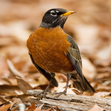
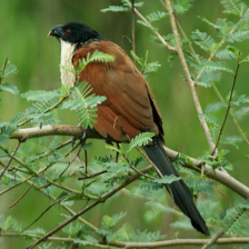
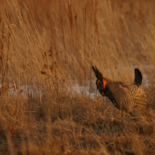
(a) Landbirds on Land

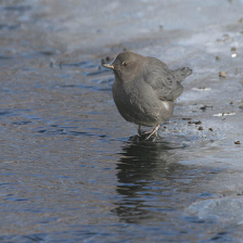
(b) Landbirds on Water

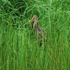
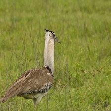
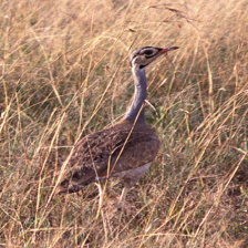
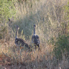
(c) Waterbirds on Land

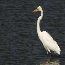
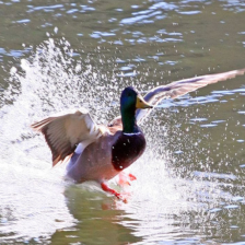
(d) Waterbirds on Water

Figure 3: Examples from Bird Groups

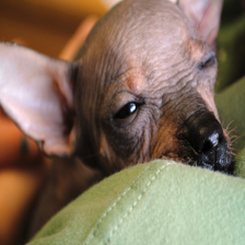
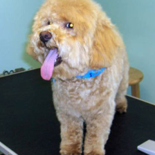
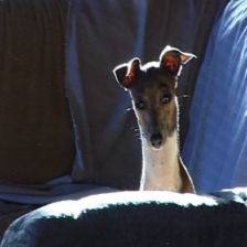
(a) Small Dogs Indoor

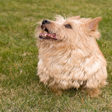
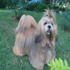
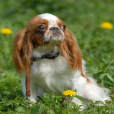
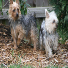
(b) Small Dogs Outdoor

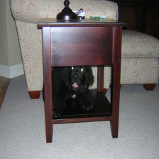
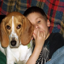
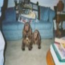
(c) Big Dogs Indoor

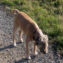
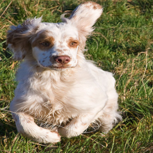
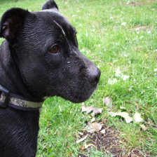
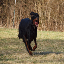
(d) Big Dogs Outdoor

Figure 4: Examples from Dog Groups

E.2 Hyperparameters

ERM We use SGD with learning rate 0.001, weight decay 0.0001, batch size 128 and momentum 0.9 as the optimizer. The model is trained for 100 epochs with early stopping.

JTT The hyperparameters used for JTT group inference and training are described below.

• During the group inference phase, we train a reference ERM model using an SGD optimizer with a learning rate of 0.001, weight decay of 0.0001, momentum of 0.9, and batch size of 128. We train the model for 7 inference epochs and upsample the error sets by 100 times.

• During the training phase, we train an ERM model with the same hyperparameters for 100 epochs.

EIIL The hyperparameters used for group inference and robust retraining are described below.

• During the group inference phase, we train a reference ERM model using an SGD optimizer with a learning rate of 0.001, weight decay of 0.0001, batch size of 128, and momentum of 0.9 for 1 epoch. Then we optimize the EI objective with a learning rate 0.01 for 20,000 steps using the Adam optimizer.

• During the robust training phase, we apply GroupDRO and use SGD with learning rate 0.001, weight decay 0.0001, batch size 128 and momentum 0.9 as the optimizer. The model is trained for 100 epochs with early stopping.

SPARE The hyperparameters used for group inference and robust retraining are described below.

• During the group inference phase, we train a reference ERM model using an SGD optimizer with a learning rate of 0.001, weight decay of 0.0001, batch size of 128, and momentum of 0.9 for 15 epochs.

• During the robust training phase, we use SGD with a learning rate of 0.001, weight decay of 0.0001, batch size of 128, and momentum of 0.9 as the optimizer and a sampling weight of 2 for importance sampling. The model is trained for 100 epochs with early stopping.

DFR The hyperparameters used for ERM training and last layer retraining are described below.

• ERM training: We use SGD with learning rate 0.001, weight decay 0.0001, batch size 128, momentum 0.9 as the optimizer. The model is trained for 100 epochs without early stopping in both settings.

• Last layer retraining with DFR. Our implementation automatically finds the optimal hyperparameter C (which represents the inverse of the $\ell_{1}$ regularization strength as in sklearn) based on a validation set. Therefore, we set the search range for C as $\{0.1,0.7,0.3,0.1,0.07,0.03,0.01\}$.

DISPEL The hyperparameters used for ERM training and last layer retraining are described below.

• ERM training: We use SGD with learning rate 0.001, weight decay 0.0001, batch size 128, momentum 0.9 as the optimizer. The model is trained for 100 epochs without early stopping in both settings.

• Last layer retraining with DISPEL. Our implementation automatically finds the optimal hyperparameter C (which represents the inverse of the $\ell_{1}$ regularization strength as in sklearn) and $s$ based on a validation set. We set the search range for C as $\{0.1,0.7,0.3,0.1,0.07,0.03,0.01\}$, and for $s$ as $\{1.0,0.99,0.98,0.97,0.96\}$.

GroupDRO During the robust training phase, we train the model from randomly initialized network parameters using SGD as the optimizer with a learning rate of 0.001, weight decay of 0.0001, batch size of 128, and momentum of 0.9. The model is trained for 100 epochs, and early stopping is applied based on the performance on the validation set.

Appendix F Additional Requirements for Dataset Publications

1. Submission introducing new datasets must include the following in the supplementary materials:

   1. Dataset documentation and intended uses. Recommended documentation frameworks include datasheets for datasets, dataset nutrition labels, data statements for NLP, and accountability frameworks.

      Dataset Nutrition Label: https://datanutrition.org/labels/v3/?id=0f6c3ec2-3613-4d1b-a502-4118b65ba5bd

   2. URL to website/platform where the dataset/benchmark can be viewed and downloaded by the reviewers.

      Link to explore dataset and benchmark: https://github.com/BigML-CS-UCLA/SpuCo

   3. Author statement that they bear all responsibility in case of violation of rights, etc., and confirmation of the data license.

      We, the authors, hereby confirm that we bear all responsibility in case of any violation of rights, intellectual property, or any other legal infringement that may occur as a result of the use of the provided data or information.

   4. Hosting, licensing, and maintenance plan. The choice of hosting platform is yours, as long as you ensure access to the data (possibly through a curated interface) and will provide the necessary maintenance.

      MNIST is hosted by torchvision and SpuCoMNIST is created dynamically using this base dataset, thus the hosting is guaranteed by existing sources. The subset of ImageNet images in SpuCoAnimals are hosted on UCLA’s Box servers and will be auto-downloaded by SpuCo when the dataset is loaded. The dataset and benchmark will be maintained by the authors.

2. To ensure accessibility, the supplementary materials for datasets must include the following:

   1. Links to access the dataset and its metadata. This can be hidden upon submission if the dataset is not yet publicly available but must be added in the camera-ready version. In select cases, e.g when the data can only be released at a later date, this can be added afterward. Simulation environments should link to (open source) code repositories.

      Link to download dataset and benchmark: https://github.com/BigML-CS-UCLA/SpuCo

   2. The dataset itself should ideally use an open and widely used data format. Provide a detailed explanation on how the dataset can be read. For simulation environments, use existing frameworks or explain how they can be used.

      The subset of images used from ImageNet are stored in jpg format compresses into a tar.gz file.

   3. Long-term preservation: It must be clear that the dataset will be available for a long time, either by uploading to a data repository or by explaining how the authors themselves will ensure this.

   4. Explicit license: Authors must choose a license, ideally a CC license for datasets, or an open source license for code (e.g. RL environments).

   5. Add structured metadata to a datasets meta-data page using Web standards (like schema.org and DCAT): This allows it to be discovered and organized by anyone. If you use an existing data repository, this is often done automatically.

   6. Highly recommended: a persistent dereferenceable identifier (e.g. a DOI minted by a data repository or a prefix on identifiers.org) for datasets, or a code repository (e.g. GitHub, GitLab,…) for code. If this is not possible or useful, please explain why.

      For the above answers: https://github.com/BigML-CS-UCLA/SpuCo

3. For benchmarks, the supplementary materials must ensure that all results are easily reproducible. Where possible, use a reproducibility framework such as the ML reproducibility checklist, or otherwise guarantee that all results can be easily reproduced, i.e. all necessary datasets, code, and evaluation procedures must be accessible and documented.

   The benchmark, datasets, scripts to run the benchmark are available at https://github.com/BigML-CS-UCLA/SpuCo. The hyperparameters used to achieve the results in this paper are presented in previous sections of the appendix.

References

- Arjovsky et al. (2019) Martin Arjovsky, Léon Bottou, Ishaan Gulrajani, and David Lopez-Paz. Invariant risk minimization. arXiv preprint arXiv:1907.02893, 2019.
- Byrd and Lipton (2019) Jonathon Byrd and Zachary Lipton. What is the effect of importance weighting in deep learning? In International conference on machine learning, pages 872–881. PMLR, 2019.
- Creager et al. (2021) Elliot Creager, Jörn-Henrik Jacobsen, and Richard Zemel. Environment inference for invariant learning. In International Conference on Machine Learning, pages 2189–2200. PMLR, 2021.
- Deng et al. (2023) Yihe Deng, Yu Yang, Baharan Mirzasoleiman, and Quanquan Gu. Robust learning with progressive data expansion against spurious correlation. arXiv preprint arXiv:2306.04949, 2023.
- Kirichenko et al. (2022) Polina Kirichenko, Pavel Izmailov, and Andrew Gordon Wilson. Last layer re-training is sufficient for robustness to spurious correlations. arXiv preprint arXiv:2204.02937, 2022.
- Li et al. (2023) Zhiheng Li, Ivan Evtimov, Albert Gordo, Caner Hazirbas, Tal Hassner, Cristian Canton Ferrer, Chenliang Xu, and Mark Ibrahim. A whac-a-mole dilemma: Shortcuts come in multiples where mitigating one amplifies others. In Proceedings of the IEEE/CVF Conference on Computer Vision and Pattern Recognition (CVPR), pages 20071–20082, June 2023.
- Liu et al. (2021) Evan Z Liu, Behzad Haghgoo, Annie S Chen, Aditi Raghunathan, Pang Wei Koh, Shiori Sagawa, Percy Liang, and Chelsea Finn. Just train twice: Improving group robustness without training group information. In International Conference on Machine Learning, pages 6781–6792. PMLR, 2021.
- Liu et al. (2015) Ziwei Liu, Ping Luo, Xiaogang Wang, and Xiaoou Tang. Deep learning face attributes in the wild. In Proceedings of International Conference on Computer Vision (ICCV), December 2015.
- Lynch et al. (2023) Aengus Lynch, Gbètondji JS Dovonon, Jean Kaddour, and Ricardo Silva. Spawrious: A benchmark for fine control of spurious correlation biases. arXiv preprint arXiv:2303.05470, 2023.
- Nam et al. (2022) Junhyun Nam, Jaehyung Kim, Jaeho Lee, and Jinwoo Shin. Spread spurious attribute: Improving worst-group accuracy with spurious attribute estimation. arXiv preprint arXiv:2204.02070, 2022.
- Radford et al. (2021) Alec Radford, Jong Wook Kim, Chris Hallacy, Aditya Ramesh, Gabriel Goh, Sandhini Agarwal, Girish Sastry, Amanda Askell, Pamela Mishkin, Jack Clark, Gretchen Krueger, and Ilya Sutskever. Learning transferable visual models from natural language supervision, 2021.
- Russakovsky et al. (2015) Olga Russakovsky, Jia Deng, Hao Su, Jonathan Krause, Sanjeev Satheesh, Sean Ma, Zhiheng Huang, Andrej Karpathy, Aditya Khosla, Michael Bernstein, Alexander C. Berg, and Li Fei-Fei. Imagenet large scale visual recognition challenge, 2015.
- Sagawa et al. (2020) Shiori Sagawa, Pang Wei Koh, Tatsunori B. Hashimoto, and Percy Liang. Distributionally robust neural networks for group shifts: On the importance of regularization for worst-case generalization, 2020.
- Selvaraju et al. (2017) Ramprasaath R Selvaraju, Michael Cogswell, Abhishek Das, Ramakrishna Vedantam, Devi Parikh, and Dhruv Batra. Grad-cam: Visual explanations from deep networks via gradient-based localization. In Proceedings of the IEEE international conference on computer vision, pages 618–626, 2017.
- Xue et al. (2023) Yihao Xue, Ali Payani, Yu Yang, and Baharan Mirzasoleiman. Eliminating spurious correlations from pre-trained models via data mixing. arXiv preprint arXiv:2305.14521, 2023.
- Yang et al. (2023) Yu Yang, Eric Gan, Gintare Karolina Dziugaite, and Baharan Mirzasoleiman. Identifying spurious biases early in training through the lens of simplicity bias. arXiv preprint arXiv:2305.18761, 2023.
- Zhang et al. (2022) Michael Zhang, Nimit S Sohoni, Hongyang R Zhang, Chelsea Finn, and Christopher Ré. Correct-n-contrast: A contrastive approach for improving robustness to spurious correlations. arXiv preprint arXiv:2203.01517, 2022.