LVM-Med: Learning Large-Scale Self-Supervised Vision Models for Medical Imaging via Second-order Graph Matching

Abstract

Obtaining large pre-trained models that can be fine-tuned to new tasks with limited annotated samples has remained an open challenge for medical imaging data. While pre-trained deep networks on ImageNet and vision-language foundation models trained on web-scale data are prevailing approaches, their effectiveness on medical tasks is limited due to the significant domain shift between natural and medical images. To bridge this gap, we introduce LVM-Med, the first family of deep networks trained on large-scale medical datasets. We have collected approximately $1.3$ million in medical images from 55 publicly available datasets, covering a large number of organs and modalities such as CT, MRI, X-ray, and Ultrasound. We benchmark several state-of-the-art self-supervised algorithms on this dataset and propose a novel self-supervised contrastive learning algorithm using a graph matching formulation. The proposed approach makes three contributions: (i) it integrates prior pair-wise image similarity metrics based on local and global information; (ii) it captures the structural constraints of feature embeddings through a loss function constructed via a combinatorial graph-matching objective; and (iii) it can be trained efficiently end-to-end using modern gradient-estimation techniques for black-box solvers. We thoroughly evaluate the proposed LVM-Med on $15$ downstream medical tasks ranging from segmentation and classification to object detection, and both for the in and out-of-distribution settings. LVM-Med empirically outperforms a number of state-of-the-art supervised, self-supervised, and foundation models. For challenging tasks such as Brain Tumor Classification or Diabetic Retinopathy Grading, LVM-Med improves previous vision-language models trained on 1 billion masks by 6-7$\%$ while using only a ResNet-50. We release pre-trained models at this link https://github.com/duyhominhnguyen/LVM-Med.

1 Introduction

Constructing large-scale annotated medical image datasets for training deep networks is challenging due to data acquisition complexities, high annotation costs, and privacy concerns [1, 2]. Vision-language pretraining has emerged as a promising approach for developing foundational models that support various AI tasks. Methods such as CLIP [3], Align [4], and Flava [5] propose a unified model trained on large-scale image-text data, showing exceptional capabilities and performance across various tasks. However, their effectiveness in the medical domain still remains unclear. A recent work SAM [6] trains large vision models on over one billion annotated masks from 11M natural images, enabling interactive segmentation. Nevertheless, SAM’s zero-shot learning performance is moderate on other datasets [7, 8], highlighting the need for fine-tuning to achieve satisfactory results [9].

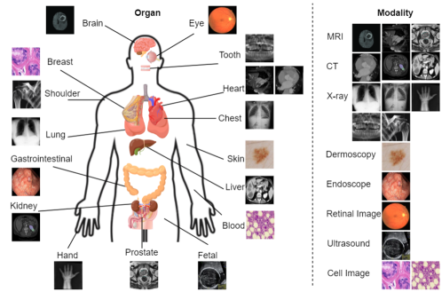
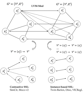
Figure 1: (left) Overview of the body organs and modalities in our collected dataset; (right) LVM-Med unifies and extends contrastive and instance-based self-supervised learning approaches by specifying graph’s properties.

To facilitate the development of foundation models in the medical domain, we make two major contributions. First, we have curated a vast collection of 55 publicly available datasets, resulting in approximately 1.3 million medical images covering various body organs and modalities such as CT, MRI, X-ray, ultrasound, and dermoscopy, to name a few. Second, we propose LVM-Med, a novel class of contrastive learning methods, utilizes pre-trained ResNet-50 and a ViT network SAM[10]. We evaluate various instances of LVM-Med relative to popular supervised architectures and vision-language models across $15$ medical tasks. To our best knowledge, this is the first time such a large-scale medical dataset has been constructed and used to investigate the capabilities of SSL algorithms.

LVM-Med incorporates a second-order graph-matching formulation, which subsumes and extends a large class of contrastive SSL methods. Given a batch of images, two random transformations are applied to each image, and the resulting transformed images are then fed to an image encoder. The embedding vectors obtained from images in a batch are used to construct two graphs where vertices represent pairs of transformed images generated from the same original one. Through solving a graph-matching problem [11, 12], we learn feature representation such that their encoding serves as suitable priors for a global solution of the graph-matching objective. This approach is distinct from prior contrastive learning methods that focus on merely optimizing pair-wise distances [13, 14] between transformed images or learning contrastive distances with positive and negative samples [15, 16, 17, 18, 19]. It is worthwhile noting that previous contrastive learning methods are special instances of our general framework (Figure (1), right).

LVM-Med has several advantages over existing approaches. First, it integrates advanced pair-wise image similarity taken from prior SSL methods into vertex affinities, resulting in both global and local information that can be efficiently fused. Second, it uncovers underlying structures of feature embeddings by utilizing edge constraints, enhancing robustness in the presence of similar entities in medical datasets. Third, though combinatorial problems are typically non-differentiable, LVM-Med can efficiently calculate gradients through the discrete combinatorial loss function using modern implicit maximum likelihood estimation techniques. Consequently, LVM-Med can scale successfully on large-scale data. In a wide range of $15$ medical experiments, LVM-Med sets a new state-of-the-art in fully fine-tuning or prompt-based segmentation, linear and fully fine-tuning image classification, and domain generalization, outperforming several vision-language models trained on a hundred million image-text instances.

We summarize major contributions in this work, including:

1. We present a collection of large-scale medical datasets, serving as a resource for exploring and evaluating self-supervised algorithms.

2. We propose LVM-Med, a novel SSL approach based on second-order graph matching. The proposed method is flexible in terms of integrating advanced pair-wise image distance and being able to capture structural feature embedding through the effective utilization of second-order constraints within a global optimization framework.

3. On both ResNet-50 and ViT architectures, LVM-Med consistently outperforms multiple existing self-supervised learning techniques and foundation models across a wide range of downstream tasks.

2 Related Work

2.1 Self-supervised learning in medical image analysis

The latest approaches of global feature SSL rely on shared embedding architecture representations that remain invariant to different viewpoints. The variation lies in how these methods prevent collapsing solutions. Clustering methods [20, 21, 22] constrain a balanced partition of the samples within a set of cluster assignments. Contrastive methods [15, 16, 17, 18] uses negative samples to push far away dissimilar samples from each other through contrastive loss, which can be constructed through memory bank [23], momentum encoder [24], or graph neural network [19]. Unlike contrastive learning, instant-based learning depends on maintaining the informational context of the feature representations by either explicit regularization [13, 25] or architectural design [26, 27]. Our work relates to contrastive and instance-based learning, where a simplified graph-matching version of 1-N or 1-1 reverts to these approaches.

In contrast to global methods, local methods specifically concentrate on acquiring a collection of local features that depict small portions of an image. A contrastive loss function can be used on those feature patches at different criteria such as image region levels [28], or feature maps [29, 14]. These strategies are also widely applied in the medical context, thereby pre-text tasks based on 3D volume’s properties, such as reconstructing the spatial context [30], random permutation prediction [31] and self-restoration [32, 33], are proposed. Our LVM-Med model on this aspect can flexible unifying both global and local information by adding them to the affinities matrixes representing the proximity of two graphs, enhancing expressive feature representations.

2.2 Vision-language foundation models

In order to comprehend the multi-modal world using machines, it is necessary to create foundational models that can operate across diverse modalities and domains [34]. CLIP [3] and ALIGN [4] are recognized as groundbreaking explorations in foundation model development. These models demonstrate exceptional proficiency in tasks such as cross-modal alignment and zero-shot classification by learning contrastive pretraining on extensive image-text pairs from the web, despite the presence of noise. To further support multi-modal generation tasks such as visual question answering or video captioning, recent works such as FLAVA [5] and OmniVL [35] are designed to learn cross-modal alignment as well as image-video language models. Conversely, the SAM model [6] utilized a supervised learning strategy with over $1$ billion masks on $11$ million user-prompt interactions and achieved impressive zero-shot segmentation performance on unseen images. While many efforts have been proposed for natural image domains, limited research has been conducted on large-scale vision models for medical imaging. This motivated us to develop the LVM-Med model.

2.3 Graph matching in visual computing

Graph matching is a fundamental problem in computer vision, which aims to find correspondences between elements of two discrete sets, such as key points in images or vertices of 3D meshes, and used in numerous vision tasks, including 3D vision [36, 37], tracking [38, 39], shape model learning [40, 41], and many others [42, 43, 44, 45]. In this framework, the vertices of the matched graphs correspond to the elements of the discrete sets to be matched. Graph edges define the cost structure of the problem, namely, second order, where pairs of matched vertices are penalized in addition to the vertex-to-vertex matchings. This allows us to integrate the underlying geometrical relationship between vertices into account but also makes the optimization problem NP-hard. Therefore, many approximate approaches have been proposed to seek acceptable suboptimal solutions by relaxing discrete constraints [46, 47]. In other directions, gradient estimation techniques for black-box solvers are employed to make the hybrid discrete-continuous matching framework be differentially end-to-end [48, 49, 50]. Our LVM-Med follows the latter direction and, for the first time, presents the formulation of contrastive learning as a second-order graph-matching problem.

3 Methodology

3.1 Dataset construction

We provide detailed information about the collected datasets in the Appendix. The data was collected from publicly available resources, which include a diverse set of modalities and body organs as illustrated in Figure 1 (left). The data format is a combination of 2D images and 3D volumes as well as X-ray, MRI, CT, Ultrasounds, etc. For datasets whose data dimensions are 3D volumes, we slice them into 2D images. To avoid potential test data leaking for downstream tasks, we use the default training partition in each dataset; otherwise, we randomly sample with $20\%$ total images. In total, we obtain approximately $1.3$ million images. More statistics on the dataset are presented in the Appendix.

3.2 Contrastive learning as graph matching

Figure 2 provides an illustration of our LVM-Med method, which learns the feature representation $f_{\theta}$ by matching two distorted views derived from the same input image through a graph-matching formulation. Below we describe in detail each component.

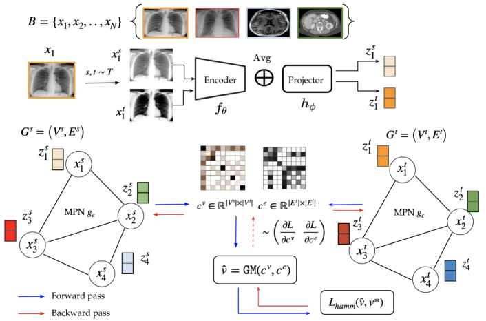
Figure 2: LVM-Med Overview. $\mathrm{Avg}$ is the average pooling layer, MPN denotes for message passing network, $\mathtt{GM}$ indicates the combinatorial solver, and $\left(c^{v},c^{e}\right)$ represents vertex and edge affinity matrices. For each image $\bm{x}_{i}$ in batch size, we generated two distorted versions and fed them into the feature representation $f_{\theta}$ and another projector $h_{\theta}$. The obtained embeddings $\bm{z}_{i}^{\ell},\ \ell\in(s,t)$ are used to build two graphs $G^{s},G^{t}$. We further design a message passing network $g_{\epsilon}$ that aggregate feature per node by their neighbor information. Then we compute vertex and edge affinities $\bm{c}^{v},\bm{c}^{e}$ and use them to solve the graph matching. The output afterward is compared with pairs of ground truth $\left(\bm{x}_{i}^{s},\bm{x}_{i}^{t}\right),i\in(1,..,N)$ representing distorted images generated from the same sample. In the backward pass, we use modern gradient-estimation techniques to approximate $\frac{\partial L}{\partial\bm{c}^{v}}$ and $\frac{\partial L}{\partial\bm{c}^{e}}$ .

3.2.1 Graph construction on feature embedding

Given a batch of $N$ images $\bm{B}=\{\bm{x}_{1},\,\bm{x}_{2},\,..,\bm{x}_{N}\}$ sampled from a dataset, we generate for each image $\bm{x}_{i}\in\bm{B}$ two transformed images $\bm{x}_{i}^{s}$ and $\bm{x}_{i}^{t}$ by using two transformations $s,t\sim T$ sampled from $T$, a set of pre-defined image transformations. After the transformations, each image is of shape $(C\times H\times W)$, where $C$ is the number of channels and $(H,W)$ the original spatial dimensions. These distorted images are fed into an encoder $f_{\theta}:\mathbb{R}^{C\times H\times W}\rightarrow\mathbb{R}^{D\times R\times S}$ to produce two representations $\bm{y}_{i}^{s}=f_{\theta}(\bm{x}_{i}^{s})$ and $\bm{y}_{i}^{t}=f_{\theta}(\bm{x}_{i}^{t})$ where $D$ is the number of feature channels and $(R,S)$ are the spatial dimensions of the feature map. On each such representation, we perform an average pooling operation $\mathrm{Avg}:\mathbb{R}^{D\times R\times S}\rightarrow\mathbb{R}^{D}$ followed by another projection $h_{\phi}:\mathbb{R}^{D}\rightarrow\mathbb{R}^{F}$ to form two feature embeddings $\bm{z}_{i}^{s}=h_{\phi}(\mathrm{Avg}(\bm{y}_{i}^{s}))$, and $\bm{z}_{i}^{t}=h_{\phi}(\mathrm{Avg}(\bm{y}_{i}^{t}))\in\mathbb{R}^{F}$ with $F<D$.

Given a set of embeddings for a batch $\bm{B}$, we construct two graphs $G^{s}$ and $G^{t}$ where, for each pair $(\bm{x}_{i}^{s},\bm{x}_{i}^{t})$ of corresponding distorted images, we add a node representing $\bm{x}_{i}^{s}$ to $G^{s}$ and a node representing $\bm{x}_{i}^{t}$ to $G^{t}$. Hence, for each $\ell\in\{s,t\}$, we construct a graph $G^{\ell}=(V^{\ell},E^{\ell})$ with $V^{\ell}=\{\bm{x}_{1}^{\ell},...,\bm{x}_{N}^{\ell}\}$ the set of vertices and $E^{\ell}$ the set of edges $e_{ij}^{\ell}=(\bm{x}_{i}^{\ell},\bm{x}_{j}^{\ell})$. The node-level feature matrix is given by $\bm{X}^{\ell}=\left[\bm{z}_{1}^{\ell};...;\bm{z}_{N}^{\ell}\right]\in\mathbb{R}^{N\times F}$ which associates each vertex $\bm{x}_{i}^{\ell}$ with its feature embedding $\bm{z}_{i}^{\ell}$. We create edges for each graph $G^{\ell}$ through a $k$-nearest neighbors algorithm using the feature matrix $\bm{X}^{\ell}$. The adjacency matrix $\bm{A}^{\ell}\in\mathbb{R}^{N\times N}$ is defined as $A_{ij}^{\ell}=1$ if $e_{ij}^{\ell}\in E^{\ell}$ and $A_{ij}=0$ otherwise. With the two graph structures given, we obtain a node-attributed graph $G^{\ell}=(V^{\ell},\bm{A}^{\ell},\bm{X}^{\ell})$ on which a graph neural network $g_{\varepsilon}$ is used to aggregate the nodes’ features. In particular, $g_{\varepsilon}$ computes an embedding $\hat{\bm{Z}}^{\ell}=g_{\varepsilon}(\bm{X}^{\ell},\bm{A}^{\ell})$ by performing message passing operations. We set $g_{\varepsilon}$ to be a graph convolutional network [51, 52] consisting of $l+1$ layers $g_{\varepsilon}=\{g_{l},g_{l-1},..,g_{0}\}$ where the output of layer $l$ is computed as

$$H_{l}^{\ell}=\sigma\left(\tilde{D}^{-\frac{1}{2}}(\bm{A}^{\ell}+\bm{I}_{N})\tilde{D}^{-\frac{1}{2}}H_{l-1}^{\ell}g_{l-1}\right),$$ (1)

where $\bm{I}_{N}$ is the identity matrix modeling self-connections; $\tilde{D}$ is a diagonal matrix with $\tilde{D}_{ii}=\sum_{j}{\bm{A}}_{ij}^{\ell}$; $g^{l-1}$ are the trainable parameters for each layer; $\sigma(\cdot)$ is an activation function; and $H_{0}^{\ell}=\bm{X}^{\ell}$. We use the outputs of the last layer as embeddings for the nodes, that is, $\hat{\bm{Z}}^{\ell}=H_{l}^{\ell}\in\mathbb{R}^{N\times F}$ given the shared graph network $g_{\varepsilon}$.

We now have two graphs $G^{s},G^{t}$ with node attribute matrices $\hat{\bm{Z}}^{s},\,\hat{\bm{Z}}^{t}$, the outputs of the graph neural networks. Next, a graph-matching problem is constructed and solved where the gold matching is given by the pairs $(\bm{x}_{i}^{s},\bm{x}_{i}^{t})\ \ \forall i\in\{1,..,N\}$.

3.2.2 Learning affinities with global and local context

To represent potential connections for a pair of node $(\bm{x}_{i}^{s},\bm{x}_{a}^{t})$ where $\bm{x}_{i}^{s}\in G^{s},\ \bm{x}_{a}^{t}\in G^{t}$, we design a vertex affinity matrix $\bm{c}^{v}\in\mathbb{R}^{|V^{s}||V^{t}|}$ where $c_{ia}^{v}$ is the prior (feature-based) similarity between $\bm{x}_{i}^{s}$ and $\bm{x}_{a}^{t}$. An advantage of our formulation is its ability to integrate advanced pair-wise distance can be smoothly integrated to $c_{ia}^{v}$, resulting in more expressive proximity representation. In particular, we leverage both global and local consistency derived from feature embeddings of distorted images. The global distance used in several prior works can be computed as $c_{ia}^{{glo}}(\bm{x}_{i}^{s},\bm{x}_{a}^{t})=\cos(\hat{\bm{z}}_{i}^{s},\hat{\bm{z}}_{a}^{t})$ where $\cos(\cdot)$ denotes cosine similarity; $\hat{\bm{z}}_{m}^{\ell}$ is the embedding of $\bm{x}_{m}^{\ell}\left(\ell\in\{s,t\},\ m\in\{i,a\}\right)$ obtained after message passing in Eq. (1).

Compared to global methods that implicitly learn features for the entire image, local methods concentrate on explicitly learning a specific group of features that characterize small regions of the image. As a result, they are more effective for dense prediction tasks such as segmentation [29, 14, 53]. While recent works applied these tactics as a part of pair-wise minimization conditions [54, 28] Instead, we integrate them as a part of vertex costs $c_{ia}^{v}$ and use it to solve the graph matching problem. Indeed, we adapt both location- and feature-based local affinity computed as:

$$c_{ia}^{\,lo}(\bm{x}_{i}^{s},\bm{x}_{a}^{t})=\mathbb{E}_{p\in\bm{P}}\cos(\bm{q}_{p}^{s},\bm{q}_{\mathrm{m}(p)}^{t})+\mathbb{E}_{p\in\bm{P}}\cos(\bm{q}_{p}^{s},\bm{q}_{\mathrm{m^{\prime}}(p)}^{t})$$ (2)

where $\bm{P}=\{(r,s)|\ (r,s)\in\left[1,...,R\right]\times\left[1,..,S\right]\}$ be the set of coordinates in the feature map $\bm{y}_{i}^{s}\in\mathbb{R}^{D\times R\times S}$ of $\bm{x}_{i}^{s}$; $\bm{q}_{p}^{\ell}$ $(\ell\in\{s,t\})$ be the feature vector at position $p$; $\mathrm{m}(p)$ denote the spatial closest coordinate to $p$ in coordinates of feature map $\bm{y}_{a}^{t}$ estimated through transformations on original image $\bm{x}_{i}$; finally $\ \mathrm{m^{\prime}}(p)$ represents the closest feature vector to $p$ in $\bm{y}_{a}^{t}$ using $l^{2}$ distance. Intuitively, the local cost in Eq. (2) enforces invariance on both spatial location and between embedding space at a local scale. Our final affinity cost is computed as:

$$c_{ia}^{v}(\bm{x}_{i}^{s},\bm{x}_{a}^{t})=\alpha\left(c_{ia}^{\,glo}(\bm{x}_{i}^{s},\bm{x}_{a}^{t})\right)+(1-\alpha)\left(c_{ia}^{lo}(\bm{x}_{i}^{s},\bm{x}_{a}^{t})+c_{ia}^{lo}(\bm{x}_{a}^{t},\bm{x}_{i}^{s})\right)$$ (3)

3.2.3 Self-supervision through second-order graph matching

While the standard graph matching problem for vertex-to-vertex correspondences can be used in our setting (LAP), it fails to capture the similarity between edges. If there are duplicated entities represented by distinct nodes in the same graph, the LAP will consider them identical and skip their neighboring relations. For instance, during the image sampling, two consecutive image slides were sampled from a 3D volume, resulting in their appearances have s a small difference. In such cases, it is complicated to correctly identify those augmented images generated from the same one without using information from the relations among connected nodes in the constructed graph. To address this problem, we introduce additional edge costs $\bm{c}^{e}\in\mathbb{R}^{|E^{s}||E^{t}|}$ where $c^{e}_{ia,jb}$ represents the similarity between an edge $v_{ij}^{s}=\left(\bm{x}_{i}^{s},\bm{x}_{j}^{s}\right)\in E^{s}$ and $v_{ab}^{t}=(\bm{x}_{a}^{t},\bm{x}_{b}^{t})\in E^{t}$. These edge costs (second-order) are computed as $c_{ia,jb}^{e}=\cos((\mathbf{\hat{z}}_{i}^{s}-\mathbf{\hat{z}}_{j}^{s}),(\mathbf{\hat{z}}_{a}^{t}-\mathbf{\hat{z}}_{b}^{t}))$.

We now establish the second-order graph-matching problem. Denoting $\bm{v}=\{0,1\}^{|V^{s}||V^{t}|}$ be indicator vector of matched vertices, i.e., $v_{ia}=1$ if the vertex $\bm{x}_{i}^{s}\in V^{s}$ is matched with $\bm{x}_{a}^{t}\in V^{t}$ and $v_{ia}=0$ otherwise. The node correspondence between two graphs $G^{s}$ and $G^{t}$ that minimizes the global condition stated as:

$$\begin{array}[]{rll}&\mathtt{GM}(\bm{c}^{v},\bm{c}^{e})=\operatorname*{arg\,min}\limits_{\begin{subarray}{c}\bm{v}\in U(\textbf{1},\textbf{1})\end{subarray}}-\sum_{i,a}c^{v}_{ia}v_{ia}-\sum_{i,j,a,b}c^{e}_{ia,jb}v_{ia}v_{jb}\\ \text{where}&U(\textbf{1},\textbf{1})=\{\bm{v}\in\{0,1\}^{N\times N}|\bm{v}\textbf{1}_{N}=\textbf{1},\bm{v}^{T}\textbf{1}_{N}=\textbf{1}\}\end{array}$$ (4)

and $\textbf{1}_{N}$ be a $n$-dimension one-value vector. The constraint $U(\textbf{1},\textbf{1})$ restricts $\bm{v}$ satisfying the one-to-one matching. Essentially, the Eq. (4) solves the vertex-to-vertex correspondence problem using both node and edges affinities, which can be seen as a form of structural matching (Figure (1),right) and generally can be integrated with higher-order graph constraints as triangle connections or circles. In the experiment, we found out that Eq. (4) significantly improved downstream task performance compared to the pure linear matching approach (Table (6)). Since the Eq. 4 in general is an NP-Hard problem [55] due to its combinatorial nature, we thus use efficient heuristic solvers based on Lagrange decomposition techniques [56].

3.2.4 Backpropagating through a graph matching formulation

With $\hat{\bm{v}}=\mathtt{GM}(\bm{c}^{v},\bm{c}^{e})$ a solution obtained from the solver, we use the Hamming distance and an optimal solution $\bm{v}^{*}$ to define the following loss function

$$L(\hat{\bm{v}},\bm{v}^{*})=\hat{\bm{v}}.(1-\bm{v}^{*})+\bm{v}^{*}.(1-\hat{\bm{v}}).$$ (5)

The proposed approach aims to learn the feature representation function $f_{\theta}$ such that its output minimizes Eq. (5). However, this is a difficult problem because the partial derivatives of the loss function w.r.t vector costs $\bm{c}^{v},\bm{c}^{e}$, i.e., $\partial L/\partial\bm{c}^{v}$ and $\partial L/\bm{c}^{e}$, are zero almost everywhere [48, 57] due to the objective function in Eq. (4) being piece-wise constant, preventing direct gradient-based optimization.

To approximate the gradients required for backpropagation, we adopt IMLE [50, 58]. Let $\bm{\theta}=\left(\bm{c}^{v},\bm{c}^{e}\right)$ be the input to the combinatorial graph matching problem in Eq. (4). The core idea of IMLE is to define a probability distribution $\rho(\bm{v};\bm{\theta})$ over solutions of the combinatorial optimization problem, where the probability of a solution is proportional to its negative cost, and to estimate $\partial L/\partial\bm{\theta}$ through the gradients of the expectation $\nabla_{\bm{\theta}}\mathbb{E}_{\bm{\hat{v}}\sim\rho(\bm{v};\bm{\theta})}\left[L(\bm{\hat{v}},\bm{v}^{*})\right]$. Since exact sampling from $\rho(\bm{v};\bm{\theta})$ is typically intractable, IMLE instead chooses a noise distribution $\rho(\bm{\epsilon})$ and approximates the gradient of the expectation over $\rho(\bm{v};\bm{\theta})$ with the gradient of the expectation over $\rho(\bm{\epsilon})$

$$\nabla_{\bm{\theta}}\mathbb{E}_{\bm{\hat{v}}\sim\rho(\bm{v};\bm{\theta})}\left[L(\bm{\hat{v}},\bm{v}^{*})\right]\approx\nabla_{\bm{\theta}}\mathbb{E}_{\bm{\epsilon}\sim\rho(\bm{\epsilon})}[L(\mathtt{GM}(\bm{\theta}+\bm{\epsilon}),\bm{v}^{*})].$$

The above approximation invokes the reparameterization trick for a complex discrete distribution. A typical choice for $\rho(\bm{\epsilon})$ is the Gumbel distribution, that is, $\rho(\bm{\epsilon})\sim\mathrm{Gumbel}(0,1)$ [59]. Now, by using a finite-difference approximation of the derivative in the direction of the gradient of the loss $\nabla_{\bm{\tilde{v}}}L(\bm{\tilde{v}},\bm{v}^{*}$), we obtain the following estimation rule:

$$\nabla_{\bm{\theta}}\mathbb{E}_{\bm{\hat{v}}\sim p(\bm{v};\bm{\theta})}\left[L(\bm{\hat{v}},\bm{v}^{*})\right] \approx\mathbb{E}_{\bm{\epsilon}\sim\rho(\bm{\epsilon})}\biggl{[}\frac{1}{\lambda}\biggl{\{}\bm{\tilde{v}}-\mathtt{GM}\left(\bm{\theta}+\bm{\epsilon}-\lambda\nabla_{\bm{\tilde{v}}}L(\bm{\tilde{v}},\bm{v}^{*})\right)\biggr{\}}\biggr{]},$$ (6)

function ForwardPass($\bm{c}^{v},\bm{c}^{e}$)

   // Gumbel noise distribution sampling

   $\epsilon,\epsilon^{\prime}\sim\mathrm{Gumbel}(0,1)$

   // Graph-matching with perturbed $\left(\bm{c}^{v},\bm{c}^{e}\right)$

   $\bm{\tilde{v}}=\mathtt{GM}\left(\bm{c}^{v}+\epsilon,\bm{c}^{e}+\epsilon^{\prime}\right)$

   // Save values for the backward pass

   save $\left(\bm{c}^{v},\bm{c}^{e}\right)$, $(\epsilon,\epsilon^{\prime})$ and $\bm{\tilde{v}}$

   return $\bm{\tilde{v}}$

function BackwardPass($\nabla_{\bm{\tilde{v}}}L(\bm{\tilde{v}},\bm{v}^{*}),\lambda$)

   load $\left(\bm{c}^{v},\bm{c}^{e}\right)$, $(\epsilon,\epsilon^{\prime})$ and $\bm{\tilde{v}}$

   // Add gradient-based pertubations

   $\left(\bm{c}^{v}_{\lambda},\bm{c}^{e}_{\lambda}\right)=\left(\bm{c}^{v}+\epsilon,\bm{c}^{e}+\epsilon^{\prime}\right)-\lambda\nabla_{\bm{\tilde{v}}}L(\bm{\tilde{v}},\bm{v}^{*})$

   // Single sample gradient estimate

   $\left(\frac{\partial L}{\partial\bm{c}^{v}},\frac{\partial L}{\partial\bm{c}^{e}}\right)=\bm{\tilde{v}}-\mathtt{GM}\left(\bm{c}^{v}_{\lambda},\bm{c}^{e}_{\lambda}\right)$

   return  $\tfrac{1}{\lambda}\left(\frac{\partial L}{\partial\bm{c}^{v}},\frac{\partial L}{\partial\bm{c}^{e}}\right)$

Algorithm 1 Forward and Backward Pass for $\bm{c}^{v}$, $\bm{c}^{e}$

where $\bm{\tilde{v}}=\mathtt{GM}(\bm{\theta}+\bm{\epsilon})$, $\lambda$ is a step size of finite difference approximation. Using a Monte Carlo approximation of the above expectation, the gradient for $\bm{\theta}$ is computed as a difference of two or more pairs of perturbed graph-matching outputs. We summarize in Algorithm 1 the forward and backward steps for $\bm{c^{v}},\bm{c^{e}}$.

4 Experiments

4.1 Implementation details

Pre-training

We utilize Resnet50 [60] and Vision Transformer (ViT-B/16) [61] to train our LVM-Med. For Resnet50, we load pre-trained from ImageNet-1K [62], and SAM Encoder backbone weight [10] for ViT. The raw image is augmented to two different views by using multi-crop techniques as [14] and followed by flip (probability 50 $\%$), color jitter, random Gaussian blur, and normalization. We trained the LVM-Med with 100 epochs on the collected dataset. The batch size of $3200$ is used for ResNet50 and we reduced it to $2800$ for ViT due to memory limitation. The model is optimized with Adam [63] with an initial learning rate $2\times 10^{-3}$ and reduced halved four times. We use $16$ A100-GPUs per with $80$GB and complete the training process for LVM-Med with ResNet-50 in five days and LVM-Med with ViT encoder in seven days. Other competitor SSL methods as VicRegl, Twin-Barlon, Dino, etc, are initialized from ResNet-50 pre-trained ImageNet-1K and trained with $100$ epochs with default settings as LVM-Med.

To balance samples among different modalities, we combine over-sampling and data augmentation to increase the total samples. Specifically, new samples from minority classes are generated by duplicating images and applying random crop operations covering $85-95\%$ of image regions and then rescaling them to the original resolutions. Note that these augmentations are not used in the self-supervised algorithm (operations $s,t\sim T$) to avoid generating identical distorted versions in this sampling procedure.

Table 1: Summary of datasets and downstream tasks

Evaluation	Downstream Task Data	Modality	Nums	Task
Fine-Tuning	BraTS2018 [64]	3D MRI	285	Tumor Segmentation
Fine-Tuning	MMWHS-CT [65]	3D CT	20	Heart Structures Segmentation
Fine-Tuning	MMWHS-MRI [65]	3D MRI	30	Heart Structures Segmentation
Fine-Tuning	ISIC-2018 [66]	2D Dermoscopy	2596	Skin Leision Segmentation
Fine-Tuning	JSRT [67]	2D X-ray	247	Multi-Organ Segmentation
Fine-Tuning	KvaSir [68]	2D Endoscope	1000	Polyp Segmentation & Detection
Fine-Tuning	Drive [69]	Fundus	40	Vessel Segmentation
Fine-Tuning	BUID [70]	2D Ultrasound	647	Breast Cancer Segmentation
Linear Evaluation & Fine-Tuning	FGADR [71]	Fundus	1841	DR Grading
Linear Evaluation & Fine-Tuning	Brain Tumor Classification	2D MRI	3264	Brain Tumor Classification
Fine-Tuning	Multi-site Prostate MRI Segmentation [72]	3D MRI	116	Prostate Segmentation
Fine-Tuning	VinDr [73]	2D X-ray	18000	Lung Diseases Detection

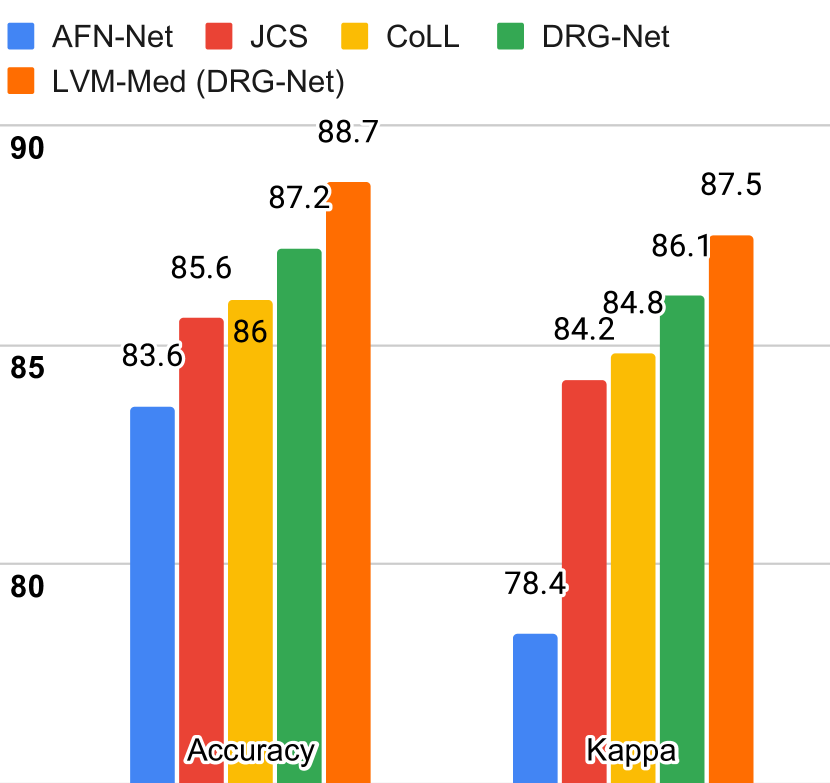
Figure 3: FGADR performance with top architectures.

Downstream Tasks

Table 1 lists the datasets and downstream tasks used in our experiments. We cover segmentation, object detection, and image classification problems. It is important to note that in most settings, we utilize simple configurations for all datasets, skipping extra pre-processing for data augmentation. For instance, overlapping image patches with stride operations in the original samples [74] to increase training data in the Drive dataset or combining different 3D MRI modalities to fuse information [75] in the BRATS-2018 are excluded in our downstream setups.

To validate LVM-Med algorithms, we compare with 2D-SSL methods trained in our dataset and foundation models like Clip [3], Align [4], Flava [5], and SAM [6] with pre-trained ViT (Bert for Align) taken from each method, respectively. During the downstream task, trained SSL weights are then extracted and attached in U-Net for ResNet50 backbone, TransUnet [76] for ViT, and then fine-tuned with training splits of each dataset. Depending on the downstream task’s properties, we apply different image resolutions and other parameters like the number of epochs and learning rate for different data domains. Details for these configurations are presented in Appendix.

4.2 2D- and 3D-based segmentation

We evaluate LVM-Med on eight medical segmentation tasks, including five 2D-based and three 3D-based segmentation. In 2D settings, we also compare with 2D supervised architectures, such as U-Net, U-Net++, Attention U-Net, etc. These networks are initialized with ResNet-50 pre-trained ImageNet. Additionally, we investigate the prompt-based segmentation settings inspired by the current success of SAM’s zero-shot learning. We utilized the ground truths and added random noise to simulate box-based user prompts as [9]. We next compare three variations of SAM: (i) freezing image and prompt encoders, only fine-tuning mask decoder; (ii) without any training and inference using box prompts; (iii) similar to (i) but replacing the original image encoder by LVM-Med’s ViT architecture taken from SAM trained in our dataset.

Table 2: Performance comparison on five 2D segmentation tasks with fully fine-tuning. Results are reported with an average 2D Dice score on three trial times. The best results in each group are in bold, the overall best value, excluding prompt-based segmentation, is underlined.

	Method	ISIC-2018 (Skin Lesion)	JSRT (Lung X-ray)	KvaSir (Polyp)	Drive (Vessel)	BUID (Breast Cancer)
	Randomly (R50)	86.16 $\pm$ 0.14	93.10 $\pm$ 0.12	62.85 $\pm$ 1.32	59.82 $\pm$ 2.00	65.54 $\pm$ 0.21
	Pre-trained ImageNet [60]	86.87 $\pm$ 0.47	94.52 $\pm$ 2.66	83.85 $\pm$ 1.32	65.12 $\pm$ 1.55	72.64 $\pm$ 1.14
	Attention-Unet [77]	86.81 $\pm$ 0.51	94.47 $\pm$ 2.71	82.23 $\pm$ 1.41	65.02 $\pm$ 1.44	72.19 $\pm$ 1.16
	U-Net ++ [78]	86.71 $\pm$ 0.49	94.32 $\pm$ 2.81	82.23 $\pm$ 1.41	65.38 $\pm$ 0.78	73.76 $\pm$ 2.83
2D Supervised Method	Trans U-Net [76]	86.60 $\pm$ 0.82	89.80 $\pm$ 0.35	67.11 $\pm$ 0.24	62.63 $\pm$ 0.24	67.90 $\pm$ 0.40
	Twin-Barlon [13]	86.01 $\pm$ 0.07	94.56 $\pm$ 3.09	83.00 $\pm$ 0.23	65.73 $\pm$ 1.46	74.46 $\pm$ 1.19
	Dino [79]	86.79 $\pm$ 0.09	94.84 $\pm$ 2.79	79.84 $\pm$ 1.62	65.39 $\pm$ 0.81	76.21 $\pm$ 0.57
	SimCLR [15]	87.28 $\pm$ 0.21	94.79 $\pm$ 2.93	82.20 $\pm$ 0.51	65.22 $\pm$ 2.18	76.52 $\pm$ 0.22
	Moco-v2 [17]	87.24 $\pm$ 0.14	94.05 $\pm$ 3.52	78.24 $\pm$ 1.35	64.92 $\pm$ 2.21	75.93 $\pm$ 1.96
	Deepcluster-v2 [20]	86.73 $\pm$ 0.42	94.79 $\pm$ 2.89	82.69 $\pm$ 0.75	64.14 $\pm$ 0.92	76.33 $\pm$ 0.99
	VicRegl [14]	86.27 $\pm$ 0.33	94.39 $\pm$ 3.25	81.93 $\pm$ 0.48	66.17 $\pm$ 0.27	75.29 $\pm$ 0.64
2D-SSL on medical	LVM-Med (R50)	87.76 $\pm$ 0.30	95.13 $\pm$ 2.64	86.76 $\pm$ 0.94	66.97 $\pm$ 0.27	78.65 $\pm$ 0.72
	Clip [3]	85.98 $\pm$ 0.19	89.00 $\pm$ 1.08	72.63 $\pm$ 0.37	63.01 $\pm$ 0.36	70.43 $\pm$ 0.24
	Flava [5]	86.42 $\pm$ 0.10	90.08 $\pm$ 0.20	69.47 $\pm$ 0.05	61.09 $\pm$ 0.45	67.54 $\pm$ 1.17
	SAM [6]	88.17 $\pm$ 0.30	90.68 $\pm$ 0.40	70.75 $\pm$ 0.60	64.04 $\pm$ 0.41	73.07 $\pm$ 0.66
Foundation Model	LVM-Med (SAM’s ViT)	88.41 $\pm$ 0.28	90.74 $\pm$ 0.47	73.10 $\pm$ 0.08	65.49 $\pm$ 0.12	77.20 $\pm$ 0.42
	SAM (fixed encoder) [9]	92.42 $\pm$ 0.12	92.89 $\pm$ 5.24	89.37 $\pm$ 0.57	59.74 $\pm$ 0.63	87.63 $\pm$ 0.67
	SAM with Prompt (no-train) [6]	55.78 $\pm$ 0.66	61.97 $\pm$ 4.48	80.77 $\pm$ 0.19	15.12 $\pm$ 0.24	78.44 $\pm$ 1.01
Prompt-based Seg.	LVM-Med (SAM’s ViT)	92.48 $\pm$ 0.07	93.74 $\pm$ 4.06	90.09 $\pm$ 0.14	63.01 $\pm$ 0.02	89.69 $\pm$ 0.61

Table 3: 3D segmentation task performance with fine-tuning on three datasets. Results are reported with an average 3D IoU on five trial times. The best results in each group and overall are in bold and underlined.

Method	BraTS	MMWHS-CT	MMWHS-MRI
3D-Transformer [80]	66.54 $\pm$ 0.40	67.30 $\pm$ 2.29	67.64 $\pm$ 2.21
I3D [81]	67.83 $\pm$ 0.75	76.63 $\pm$ 2.32	66.71 $\pm$ 1.27
NiftyNet [82]	60.78 $\pm$ 1.60	74.91 $\pm$ 2.78	64.60 $\pm$ 1.96
Med3D [83]	66.09 $\pm$ 1.35	75.01 $\pm$ 0.74	63.43 $\pm$ 0.61
Model Genesis [32]	67.96 $\pm$ 1.29	76.48 $\pm$ 2.89	74.53 $\pm$ 1.69
Universal Model [84]	72.10 $\pm$ 0.67	78.14 $\pm$ 0.77	77.52 $\pm$ 0.50
TransVW [33]	68.82 $\pm$ 0.38	79.74 $\pm$ 2.78	75.08 $\pm$ 2.04
SwinViT3D [85]	70.58 $\pm$ 1.27	70.19 $\pm$ 1.23	78.25 $\pm$ 1.66
Joint-2D-3D (Deepc) [86]	72.81 $\pm$ 0.15	83.58 $\pm$ 1.54	78.14 $\pm$ 1.32
Twin-Barlon [13]	73.30 $\pm$ 0.18	84.74 $\pm$ 1.01	76.39 $\pm$ 2.23
Dino [79]	71.72 $\pm$ 0.55	81.08 $\pm$ 1.62	70.42 $\pm$ 78.74
SimCLR [15]	73.15 $\pm$ 0.27	84.60 $\pm$ 1.11	76.54 $\pm$ 2.22
Moco-v2 [17]	71.97 $\pm$ 0.63	75.82 $\pm$ 4.20	68.29 $\pm$ 0.15
Deepcluster [20]	72.96 $\pm$ 0.51	84.03 $\pm$ 0.50	79.05 $\pm$ 1.63
VicRegl [14]	73.23 $\pm$ 0.33	84.72 $\pm$ 0.86	76.32 $\pm$ 0.78
LVM-Med (R50)	73.58 $\pm$ 0.14	84.91 $\pm$ 0.77	78.59 $\pm$ 0.84
Clip [3]	70.24 $\pm$ 1.23	78.5 $\pm$ 2.70	65.9 $\pm$ 3.98
Flava [5]	71.19 $\pm$ 0.48	78.91 $\pm$ 2.24	67.14 $\pm$ 1.20
SAM (Encoder) [6]	70.11 $\pm$ 1.45	77.8 $\pm$ 1.60	68.09 $\pm$ 5.49
LVM-Med (SAM’s ViT)	71.42 $\pm$ 0.70	80.78 $\pm$ 1.77	69.36 $\pm$ 0.18

Table 4: In-out-distribution evaluation for the segmentation task on the Prostate dataset. Results are reported with an average 2D Dice score on three training times.

Method	Multi-site Prostate Segmentation
	BMC (Based)	RUNMC	BIDMC	HK	Average
2D Supervised
Random	65.04 $\pm$ 2.07	51.44 $\pm$ 4.13	9.95 $\pm$ 13.56	12.38 $\pm$ 7.68	34.7
Pretrained ImageNet [60]	76.47 $\pm$ 1.26	62.11 $\pm$ 0.85	43.74 $\pm$ 4.38	53.90 $\pm$ 2.01	59.1
2D SSL on medical data
Twin-Barlon [13]	76.28 $\pm$ 1.76	60.09 $\pm$ 1.98	32.63 $\pm$ 12.32	34.82 $\pm$ 15.09	51.0
Dino [79]	77.90 $\pm$ 1.15	56.90 $\pm$ 1.97	21.53 $\pm$ 5.54	30.92 $\pm$ 5.41	46.8
SimCLR [15]	76.51 $\pm$ 2.07	64.10 $\pm$ 4.53	32.88 $\pm$ 5.43	42.29 $\pm$ 5.98	53.9
Moco-v2 [17]	74.40 $\pm$ 0.89	55.49 $\pm$ 5.45	27.53 $\pm$ 10.18	13.65 $\pm$ 14.33	42.8
Deepcluster [20]	77.45 $\pm$ 0.35	64.35 $\pm$ 3.15	37.73 $\pm$ 8.08	44.95 $\pm$ 8.57	56.1
Swav [21]	77.59 $\pm$ 0.61	57.61 $\pm$ 2.16	38.43 $\pm$ 12.55	44.90 $\pm$ 4.78	54.6
VicRegl [14]	74.85 $\pm$ 1.13	54.09 $\pm$ 4.35	25.56 $\pm$ 5.44	35.45 $\pm$ 13.03	47.5
LVM-Med (R50)	80.17 $\pm$ 0.55	62.48 $\pm$ 2.03	56.76 $\pm$ 6.50	52.78 $\pm$ 3.04	63.0
Prompt-based Seg.
SAM (Fixed encoder) [9]	95.50 $\pm$ 0.29	90.39 $\pm$ 0.39	91.41 $\pm$ 0.14	91.82 $\pm$ 0.26	92.28
SAM with Prompt (no-train) [6]	59.11 $\pm$ 1.55	66.95 $\pm$ 2.49	59.68 $\pm$ 0.49	57.41 $\pm$ 2.83	60.79
LVM-Med (SAM’s ViT)	95.75 +- 0.06	90.40 +- 0.36	92.03 +- 0.20	92.75 +- 0.48	92.73

In 3D settings, we segment 2D slices and merge results for a 3D volume. We also benchmarked with 3D self-supervised methods from [86]. Tables (2) and (3) show that our two versions with ResNet-50 and Sam’s ViT hold the best records in each category. For instance, we outperform 2D SSL methods trained on the same dataset, surpassing foundation models such as SAM, Flava, and Clip. In the prompt-based settings, LVM-Med also delivers better performance compared with SAM. Second, LVM-Med achieves the best overall results on seven of eight segmentation tasks, mostly held by LVM-Med with ResNet-50. The improvement gaps vary on each dataset, for e.g., from $3-5\%$ on Kvasir and BUID compared with 2D supervised methods.

4.3 Linear and finetuning image classification

We analyze LVM-Med on image classification tasks using linear probing (frozen encoders) and fully fine-tuning settings, two popular evaluations used in self-supervised learning. The experiments are conducted on the FGADR Grading and Brain tumor classification tasks. Table (5) presents the average accuracy metric on three training times. LVM-Med (ResNet-50) consistently outperforms other approaches on two datasets. For example, it is better than Clip by $10.46\%$ and $8.46\%$ on FGADR and Brain Tumor datasets with linear evaluation. In the foundation model setting, LVM-Med (ViT) also improves SAM’s results by $7.32\%$ and $4.69\%$ on FGADR with linear and fully-finetuning. Another point we observe is that the overall 2D-SSL methods based on ResNet-50 and trained on the collected medical dataset achieve higher accuracy than foundation models using ViT. We also compare LVM-Med with the top methods on the FGADR dataset, including AFN-Net [87], JCS [88], CoLL [89], and DRG-Net [90]. We choose the DRG-Net as the backbone and replace the employed encoder with our weights (R50). Figure (3) shows that LVM-Med hold the first rank overall.

Table 5: Performance comparison on linear evaluation and fine-tuning classification. The results are reported with average Accuracy on three training times.

Method	Linear Evaluation (Frozen)		Fine-tuning
	FGADR	Brain Tumor Cls.	FGADR	Brain Tumor Cls.
Twin-Barlon [13]	66.86 $\pm$ 0.41	63.03 $\pm$ 0.32	66.37 $\pm$ 0.77	74.20 $\pm$ 1.38
Dino [79]	65.98 $\pm$ 1.91	62.27 $\pm$ 0.32	67.35 $\pm$ 1.36	71.91 $\pm$ 1.55
SimCLR [15]	65.30 $\pm$ 1.70	62.52 $\pm$ 1.67	67.55 $\pm$ 0.28	73.52 $\pm$ 3.56
Moco-v2 [17]	65.98 $\pm$ 1.04	62.35 $\pm$ 1.92	67.55 $\pm$ 1.79	74.53 $\pm$ 0.43
Deepcluster [20]	65.34 $\pm$ 1.93	64.47 $\pm$ 0.55	67.94 $\pm$ 1.78	73.10 $\pm$ 0.55
VicRegl [14]	64.71 $\pm$ 0.60	59.64 $\pm$ 1.36	65.69 $\pm$ 1.46	73.18 $\pm$ 2.03
LVM-Med (R50)	68.33 $\pm$ 0.48	66.33 $\pm$ 0.31	68.32 $\pm$ 0.48	76.82 $\pm$ 2.23
Clip [3]	57.87 $\pm$ 0.50	57.87 $\pm$ 0.71	57.48 $\pm$ 0.86	34.86 $\pm$ 2.27
Flava [5]	31.87 $\pm$ 0.69	35.19 $\pm$ 0.43	57.18 $\pm$ 0.96	34.01 $\pm$ 5.97
Algin [4]	36.95 $\pm$ 1.04	30.71 $\pm$ 2.35	57.28 $\pm$ 0.97	63.96 $\pm$ 0.04
SAM [6]	55.13 $\pm$ 0.41	31.81 $\pm$ 4.26	58.75 $\pm$ 1.32	60.66 $\pm$ 1.36
LVM-Med (SAM’s ViT)	62.46 $\pm$ 0.86	59.31 $\pm$ 0.48	63.44 $\pm$ 0.73	67.34 $\pm$ 2.08

Table 6: LVM-Med ablation study. Results are reported on an average of five 2D segmentation and two linear classification tasks. The two most important factors are highlighted.

Method	Cls.(Acc)	Seg. (Dice)
LVM-Med (Full)	67.47	83.05
LVM-Med w/o second-order	62.17	80.21
LVM-Med w/o message passing	65.08	81.19
LVM-Med w/o Gumbel noise	64.32	81.37
LVM-Med w/o local similarity	65.67	81.54

4.4 Object detection & In-out-distribution evaluation

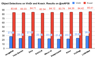
Figure 4: LVM-Med on object detection.

Figure 4 indicates our performance on the object detection task using VinDr and Kvasir datasets. We use Faster R-CNN and load ResNet-50 from 2D SSL pre-trained weights. Results are presented by Average Precision with IoU=0.5 over three training times. Compared to pre-trained Imagenet, LVM-Med still outperforms by $1$-$2\%$ though overall, our improvements are smaller than image classification and segmentation tasks.

We also validate LVM-Med performance on the in-out-distribution setting in Table (4) using the segmentation task on the Multi-Prostate dataset. We train LVM-Med and other competitors in BMC data and use the trained models to predict the remaining datasets. Both two versions of LVM-Med with ResNet-50 and ViT, on average, surpass all baselines, which validates the potential abilities of LVM-Med for the in-out-distribution problem.

4.5 Ablation study

We do the following settings to evaluate the performance of components used in LVM-Med: (i) LVM-Med without using second-order graph matching conditions, i.e., only solving vertex-to-vertex correspondence problem; (ii) LVM-Med without using message passing network $g_{\epsilon}$ in Eq. (1) to aggregate information from local connections; (iii) LVM-Med w/o using approximate gradients from Gumbel noise in Eq. (6). For this, we add a constant value to $\bm{c}^{v},\bm{c}^{e}$ as prior works [57, 49], and finally (iv) LMV-Med without using local similarity $c_{ia}^{lo}$ in Eq. (2). Other ablation studies are presented in Appendix. Table (6) indicates that all factors contribute to the final performance, wherein the second-order and Gumbel noise are the two most two important parts.

5 Conclusion

We have demonstrated that a self-supervised learning technique based on second-order graph-matching, trained on a large-scale medical imaging dataset, significantly enhances performance in various downstream medical imaging tasks compared to other supervised learning methods and foundation models trained on hundreds of millions of image-text instances. Our findings are supported by the benefits shown in two different architectures: ResNet-50 and ViT backbones, which can be used for either end-to-end or prompt-based segmentation.

Limitations and Future Work. We propose to investigate the following points to improve LVM-Med performance. Firstly, extending LVM-Med to a hybrid 2D-3D architecture to allow direct application for 3D medical tasks instead of 2D slices. Secondly, although LVM-Med with ViT backbone utilizes more total parameters, in some cases, it is less effective than LVM-Med ResNet-50. This raises the question of whether a novel approach could improve the performance of ViT architectures. Finally, integrating multi-modal information such as knowledge graphs, bio-text, or electronic health records for LVM-Med is also important to make the model more useful in real-world applications.

Supplementary Material

We present below LVM-Med pseudo-code (Section A), implementations used in downstream tasks (Section B), additional ablation studies of LVM-Med (Section C), further prompt-based segmentation results on 3D datasets, image classification benchmark (Section D), predicted masks using the user-based prompt (Section E), and finally the dataset overview (Section F).

Appendix A LVM-Med Pseudo-code

First, we provide a pseudo-code for training LVM-Med in Pytorch style:
  # $\mathtt{f_{\theta}}$: encoder network, $\mathtt{h_{\phi}}$: projector network, $\mathtt{g_{\epsilon}}$: message passing network,
# k_nodes: number of nearest neighbors, Avg: average pooling,
# pos: position of image after transform, cos: cosine similarity,
# $\mathtt{\alpha}$: coefficient trades off between global and local costs, $\mathtt{L_{2}}$: L2-distance,
# $\mathtt{\gamma}$: maximum pairs are kept, select_top: select to keep the $\mathtt{\gamma}$ best matches.

for X in loader: # load a batch X = $\mathtt{\left[x_{1},x_{2},...,x_{N}\right]}$ with N samples
     # apply two transformations s and t
     $\mathtt{X^{s},\ Pos^{s}=s(X)}$  # $\mathtt{X^{k}=\left[x_{1}^{k},x_{2}^{k},...,x_{N}^{k}\right]}$, $\mathtt{Pos^{k}=\left[pos_{1}^{k},pos_{2}^{k},...,pos_{N}^{k}\right],\ k\in\{s,t\}}$
     $\mathtt{X^{t},\ Pos^{t}=t(X)}$

     # compute feature representations
     $\mathtt{Y^{s}=f_{\theta}(X^{s});\ Y^{t}=f_{\theta}(X^{t})}$ # feature dimensions:NxDxRxS

     # applying projection
     $\mathtt{Z^{s}=h_{\phi}(Avg(Y^{s}));\ Z^{t}=h_{\phi}(Avg(Y^{t}))}$ # dimensions:NxF

     # build graph structures and message passing
     $\mathtt{G^{s}}$ = k-nearest-neighbor($\mathtt{Z^{s}}$, k_connects)
     $\mathtt{G^{t}}$ = k-nearest-neighbor($\mathtt{Z^{t}}$,k_connects)
     $\mathtt{\hat{Z}^{s}=g_{\epsilon}(G^{s},Z^{s})}$; $\mathtt{\hat{Z}^{t}=g_{\epsilon}(G^{t},Z^{t})}$

     # compute vertex and edge affinity matrices
     $\mathtt{c_{ia}^{v}=\alpha*\,cos(\hat{z}_{i}^{s},\hat{z}_{a}^{t})+(1-\alpha)*\,local\_cost(y_{i}^{s},\,y_{a}^{t},\,pos_{i}^{s},\,pos_{a}^{t})}$ # affinity $\mathtt{x_{i}^{s}}$ & $\mathtt{x_{a}^{t}}$
     $\mathtt{c^{e}_{ia,jb}=cos((\hat{z}_{i}^{s}-\hat{z}_{j}^{s}),(\hat{z}_{a}^{t}-\hat{z}_{b}^{t}))}$ # affinity between edges $\mathtt{v_{ij}^{s},v_{ab}^{t}}$
     $\mathtt{c^{v}=\{c_{ij}^{v}\}\in R^{N\times N};\ c^{e}=\{c^{e}_{ia,jb}\}\in R^{|E^{s}||E^{t}|}}$  # $\mathtt{E^{k}}$ be a set of edges in $\mathtt{G^{k},\,k\in\{s,t\}}$

     # perturbed costs with Gumbel noise
     $\mathtt{\epsilon,\epsilon^{\prime}\sim Gumbel(0,1)}$
     $\mathtt{c^{v}=c^{v}+\epsilon;\ c^{e}=c^{e}+\epsilon^{\prime}}$

     # solving graph matching and compute loss
     $\mathtt{\hat{v}=GM(c^{v},c^{e})}$
     $\mathtt{L(\hat{\bm{v}},\bm{v}^{*})=\hat{\bm{v}}.(1-\bm{v}^{*})+\bm{v}^{*}.(1-\hat{\bm{v}})}$  # compute hamming loss

     # update network
     L.backward() # approximate ($\mathtt{\partial L/\partial c^{v},\partial L/\partial c^{e}}$) by Algorithm 1.
     Update($\mathtt{g_{\epsilon}.params}$), Update($\mathtt{h_{\phi}.params}$), Update($\mathtt{f_{\theta}.params}$)

# define local_cost
def local_cost($\mathtt{y_{i}^{s},\,y_{a}^{t},\,pos_{i}^{s},\,pos_{a}^{t}}$):

     # location-based local cost
     $\mathtt{y_{i,nn}^{s}=torch.zeros\_like(y_{i}^{s})}$
     for r, s in R, S:
          r’, s’ = argmin($\mathtt{\left(L_{2}(pos_{i}^{s}[r,s],\ pos_{a}^{t}[r^{\prime},s^{\prime}]\right)}$)
          $\mathtt{y_{i,nn}^{s}[r,s]=y_{a}^{t}[r^{\prime},s^{\prime}]}$

     $\mathtt{y_{i\_fil}^{s},y_{i,nn\_fil}^{s}=select\_top\,\left(y_{i}^{s},\,y_{i,nn}^{s},\gamma\right)}$

     location_cost = cos($\mathtt{y_{i\_fil}^{s},y_{i,nn\_fil}^{s}}$)

     # featured-based local cost
     $\mathtt{y_{i,nn}^{s}=torch.zeros\_like(y_{i}^{s})}$
     for r, s in R, S:
          r’, s’ = argmin($\mathtt{\left(L_{2}(y_{i}^{s}[r,s],\ y_{a}^{t}[r^{\prime},s^{\prime}]\right)}$)
          $\mathtt{y_{i,nn}^{s}[r,s]=y_{a}^{t}[r^{\prime},s^{\prime}]}$

     $\mathtt{y_{i\_fil}^{s},y_{i,nn\_fil}^{s}=select\_top\,\left(y_{i}^{s},\,y_{i,nn}^{s},\gamma\right)}$

     feature_cost = cos($\mathtt{y_{i\_fil}^{s},y_{i,nn\_fil}^{s}}$)

     return 0.5*(location_cost + feature_cost)
 
We trained LVM-Med with graph size of $16$ nodes, each node connected to the top 5 nearest neighbors after using kNN, $\lambda$ value in Algorithm 1 is $80$, and $\alpha=0.8$ for associating global- and local-based similarities when computing $c^{v}_{ij}$. The size of projector $h_{\phi}$ is $2048\times 128$ for ResNet-50, and $768\times 128$ for ViT. We configure the message passing network $g_{\theta}$ with two convolutional layers of size $128$. For the user-based prompt version, because the SAM model [9] requires an input of shape $256\times 14\times 14$ for the mask decoder part, we add two additional convolutional layers with a kernel size of $1$ and $3$ at the end of ViT backbone to convert from shape $768\times 14\times 14$ to the target shape.

Appendix B Downstream task setups

B.1 Downstream tasks

Segmentation tasks

On 2D-based segmentation tasks, we employ U-Net architecture [91] and load ResNet-50 [60] trained by self-supervised learning algorithms as network backbones. With foundation models, we use TransUnet [76] and take pre-trained ViT models as the backbones. For the prompt-based segmentation, we follow the architecture of SAM [6] consisting of encoder, prompt, and mask decoder layers. We also fine-tune SAM where encoder and prompt networks are frozen, only learning decoder layers [9]. Our LVM-Med for prompt-based setting is similar to [9] except that we substitute SAM’s encoders with our weights. We utilize Adam optimizer for all experiments and train architectures with Dice and Cross-Entropy loss [92]. We also normalize the norm-2 of gradient values to stabilize the training step to maximize 1. Table 7 summarizes each dataset’s learning rate, number of epochs, and image resolution.

On 3D-based segmentations, we reformulate these tasks as 2D segmentation problems and make predictions on 2D slices taken from 3D volumes. Furthermore, we apply balance sampling to select equally 2D slices covering target regions and other 2D slices, not including the ground truth. Table 8 presents configurations used for 3D datasets; other settings are identical to 2D cases.

Table 7: Configurations for training 2D segmentation tasks

	ISIC-2018 (Skin Lesion)	JSRT (Lung X-ray)	KvaSir (Polyp)	Drive (Vessel)	BUID (Breast Cancer)
ResNet-50.	lr = $10^{-4}$, epochs $35$	lr = $10^{-3}$, epochs $50$	lr = $10^{-3}$, epochs $35$	lr = $10^{-3}$, epochs $50$	lr = $10^{-4}$, epochs $50$
	shape $512\times 512$	shape $224\times 224$	shape $224\times 224$	shape $224\times 224$	shape $256\times 256$
	batch size $16$	batch size $32$	batch size $64$	batch size $16$	batch size $8$
Foundation Model	lr = $10^{-4}$, epochs $100$	lr = $10^{-3}$, epochs $200$	lr = $10^{-3}$, epochs $200$	lr = $10^{-3}$, epochs $200$	lr = $10^{-4}$, epochs $200$
	shape $512\times 512$	shape $224\times 224$	shape $224\times 224$	shape $224\times 224$	shape $256\times 256$
	batch size $16$	batch size $32$	batch size $64$	batch size $16$	batch size $8$
Prompt-based Seg.	lr = $10^{-4}$, epochs $50$	lr = $3\times 10^{-4}$, epochs $50$	lr = $3\times 10^{-4}$, epochs $20$	lr = $3\times 10^{-4}$, epochs $100$	lr = $10^{-4}$, epochs $20$
	shape $1024\times 1024$	shape $1024\times 1024$	shape $1024\times 1024$	shape $1024\times 1024$	shape $1024\times 1024$
	batch size $16$	batch size $16$	batch size $16$	batch size $16$	batch size $16$

Table 8: Configurations for 3D-based-segmentation tasks

	BraTS	MMWHS-CT	MMWHS-MRI	BMC
ResNet50	lr = $15\times 10^{-4}$, epochs $20$	lr = $10^{-3}$, epochs $20$	lr = $15\times 10^{-4}$, epochs $30$	lr = $10^{-3}$, epochs $30$
	shape $224\times 224$	shape $224\times 224$	shape $224\times 224$	shape $224\times 224$
	batch size $128$	batch size $64$	batch size $64$	batch size $64$
Foundation Model	lr = $10^{-4}$, epochs $100$	lr = $10^{-4}$, epochs $100$	lr = $10^{-4}$, epochs $100$	lr = $10^{-4}$, epochs $100$
	shape $224\times 224$	shape $224\times 224$	shape $224\times 224$	shape $224\times 224$
	batch size $16$	batch size $16$	batch size $16$	batch size $16$
Prompt-based Seg.	lr = $3\times 10^{-5}$, epochs $30$	lr = $5\times 10^{-5}$, epochs $30$	lr = $3\times 10^{-5}$, epochs $30$	lr = $3\times 10^{-4}$, epochs $50$
	shape $1024\times 1024$	shape $1024\times 1024$	shape $1024\times 1024$	shape $1024\times 1024$
	batch size $16$	batch size $16$	batch size $16$	batch size $16$

Image classification tasks

We take the feature embedding outputs of each architecture and build one fully connected layer to produce desired classes for image classification tasks. We freeze the encoder layers for the linear evaluation and only train the fully connected layer. For the fully-finetuning, the whole network is trained. The Adam optimizer [63] with cross-entropy loss function and learning rates $\{5\times 10^{-4},10^{-3}\}$ are used for Brain Tumor and FGADR, respectively. To benchmark LVM-Med with other state-of-the-art methods on FGADR (Figure 3 in paper), we follow the settings of DRG-Net [90] and change their encoder layers by our networks.

Object detection

We use Faster-RCNN [93] for object detection tasks. The ResNet-50 of Faster-RCNN is replaced by pre-trained weights. In the Vin-Dr dataset, there is a total of $14$ objects for, e.g., Aortic enlargement, Atelectasis, Calcification, etc. We use image resolutions of $512\times 512$, Adam solver, and learning rate $10^{-4}$ in $40$ epochs. In the Kvasir dataset for polyp detection, we also resize images to a fixed size of $512\times 512$, employ the Adam optimizer with learning rate $2.5\times\mathrm{10}^{-4}$ and batch size $8$.

Appendix C LVM-Med ablation studies

C.1 Graph sizes and $\lambda$ in backpropagation

We provide in Figure 5 and Figure 6 LVM-Med performance when changing the number of nodes in graph construction steps $G^{s},G^{t}$ and $\lambda=80$ used in Algorithm 1 in the backpropagation step. The results are reported on the average Dice score of five 2D segmentation tasks and the average accuracy of two linear classifications on FGADR and Brain Tumor Classification. Figure 5 indicates that $16$ is the best value for both classification and segmentation. Increasing the graph’s nodes tends to decrease classification performance.

Figure 6 compared different values for $\lambda\in\{70,80,90,100\}$. We observe that $\lambda=\{80,90\}$ achieve good results for linear classification tasks though $\lambda=\{90,100\}$ decreases segmentation performance.

C.2 Performance on large- and small-scale

We investigate LVM-Med performance when reducing the number of datasets in the pre-training step. Especially, we trained LVM-Med on a small-scale with four datasets: LUNA2016 [94], LiTS2017 [95], BraTS2018 [64], and MSD (Heart) [96]. We compare this version with our default settings trained on $55$ datasets (Section F). Two models are evaluated on dice scores of five 2D segmentation tasks, the accuracy metric of two linear image classifications, and mAP50 of two object detection tasks on VinDr and Kvasir detection. Table 9 shows that LMV-Med full leads to better performance overall, especially with the classification settings; the improvement gap is around $3.6\%$. In summary, we conclude that LVM-Med is beneficial when training in large-scale medical settings.

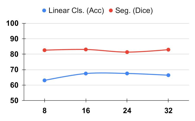
Figure 5: LVM-Med performance when varying the number of nodes in graph construction.

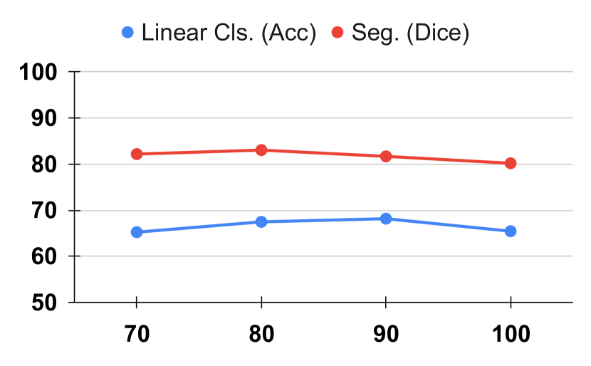
Figure 6: LVM-Med performance when varying the $\lambda$ in backpropagation step.

C.3 Performance on weighting global and local similarities

We test with different $\alpha=\{0.7,0.8,0.9\}$ which used to fuse global- and local-based similarities $c^{v}_{ij}$. Table 9 demonstrates that $\alpha=0.8$ is generally the best value in average across segmentation, classification, and object detection tasks.

Table 9: LVM-Med ablation studies trained with full data, small-scale, and different hyper-parameter $\alpha$ fusing global- and local-based similarities. Results are reported on an average of five 2D segmentation, two linear classifications, and two object detection tasks. The most impacted factors are highlighted.

Method	Cls.(Acc)	Seg. (Dice)	Detect. (mAP50)
LVM-Med (full, $\alpha=0.8$)	67.47	83.05	57.1
LVM-Med (small-scale, $\alpha=0.8$)	63.83	81.97	56.03
LVM-Med (full, $\alpha=0.7$)	65.89	82.20	56.49
LVM-Med (full, $\alpha=0.9$)	65.03	81.09	57.14

C.4 Computational complexity

We present a parameter comparison of LVM-Med with other foundation models in Table 10. Our LVM-Med model, based on ResNet-50, has significantly fewer parameters, approximately 3-4 times smaller than models such as Flava or SAM, while still maintaining competitive performance. When utilizing the ViT encoder pre-trained by the SAM method, LVM-Med’s parameters are comparable to the Flava model and slightly higher than Clip and Align by $1.03$ and $1.43$ times, respectively. However, it is important to note that both LVM-Med and SAM outperform these models by a significant margin in various settings.

Table 10: Computational complexity of our approaches and other foundation models.

Method	LVM-Med (R50)	LVM-Med (ViT)	Clip [3]	Flava [5]	Align [4]	SAM (Encoder) [6]
#Param	25.55 M	88.88 M	85.80 M	86.39 M	62.14 M	88.88 M

Appendix D Prompt-based segmentation on 3D datasets and classification tasks

We provide additional results for LVM-Med on 3D-based prompt segmentation and image classification tasks with several fully connected layers.

D.1 Promt-based Segmentation on 3D datasets

We perform experiments on three 3D datasets in Table 11, including BraTS, MMWHS-MRI, and MMWHS-CT. The setup for box prompts follows 2D segmentation cases. We discover that the LMV-Med in 3D cases consistently improves the performance of fine-tuned SAM [9] as in 2D settings and attains a large margin compared with SAM without training [6]. This evidence thus confirms that LVM-Med is also effective under prompt-based scenarios.

Table 11: Prompt-based segmentation on 3D datasets.

	Method	BraTS	MMWHS-MRI	MMWHS-CT
Prompt-based Seg.	SAM (fixed encoder) [9]	85.37 $\pm$ 0.07	77.64 $\pm$ 1.14	76.61 $\pm$ 1.91
	SAM with Prompt (no-train) [6]	38.97 $\pm$ 0.21	59.74 $\pm$ 0.76	50.25 $\pm$ 0.33
	LVM-Med (SAM’s ViT)	85.76 $\pm$0.07	78.91 $\pm$ 0.80	78.03 $\pm$ 0.93

D.2 Image classification

We aim to inspect whether foundation models improve their performance given more fully connected layers for image classification tasks with both frozen encoders or fully fine-tuning. For each method in this category and our LVM-Med (ResNet-50 and ViT), we configure two fully connected layers with sizes $512-256$ and $512-128$ for the Brain and FGADR respectively that map from the output dimension of each network to a number of desired classes. Table 12 presents obtained results where new settings are highlighted in color. We notice the following points. (i) Firstly, using more fully connected layers tends to improve the performance of foundation models, especially on linear evaluation. For e.g., the Clip increases from $4.79\%-9.98\%$ on FGADR and Brain Tumor classification tasks, respectively. Similarly, our LVM-Med with SAM’s ViT also achieves better results by approximately $1.37\%$ and $4.82\%$ on those tasks. (ii) Secondly, LVM-Med overall attains the best results in four settings using linear or several fully connected layers with ResNet-50. LVM-Med with ViT architecture also delivers the best records on three of four test cases compared with foundation models.

Table 12: Comparing SSL approaches and Foundation models on classification tasks with two evaluation protocols, Linear evaluation and full Fine-tuning. Settings used with several fully connected layers are in cyan. The best results in 2D-SSL and foundation models (two fully connected layers) are in bold; the best results overall are in bold and underlined.

	Method	Linear Evaluation (Frozen)		Fine-tuning
		FGADR (DR Grading)	Brain Tumor Class.	FGADR (DR Grading)	Brain Tumor Class.
2D-SSL on medical	Twin-Barlon [13]	66.86 $\pm$ 0.41	63.03 $\pm$ 0.32	66.37 $\pm$ 0.77	74.20 $\pm$ 1.38
	Dino [79]	65.98 $\pm$ 1.91	62.27 $\pm$ 0.32	67.35 $\pm$ 1.36	71.91 $\pm$ 1.55
	SimCLR [15]	65.30 $\pm$ 1.70	62.52 $\pm$ 1.67	67.55 $\pm$ 0.28	73.52 $\pm$ 3.56
	Moco-v2 [17]	65.98 $\pm$ 1.04	62.35 $\pm$ 1.92	67.55 $\pm$ 1.79	74.53 $\pm$ 0.43
	Deepcluster [20]	65.34 $\pm$ 1.93	64.47 $\pm$ 0.55	67.94 $\pm$ 1.78	73.10 $\pm$ 0.55
	VicRegl [14]	64.71 $\pm$ 0.60	59.64 $\pm$ 1.36	65.69 $\pm$ 1.46	73.18 $\pm$ 2.03
	LVM-Med (R50)	68.33 $\pm$ 0.48	66.33 $\pm$ 0.31	68.32 $\pm$ 0.48	76.82 $\pm$ 2.23
		66.67 $\pm$ 0.84	74.70 $\pm$ 0.84	70.58 $\pm$ 0.36	78.77 $\pm$ 0.78
Foundation Model	Clip [3]	57.87 $\pm$ 0.50	57.87 $\pm$ 0.71	57.48 $\pm$ 0.86	34.86 $\pm$ 2.27
		62.66 $\pm$ 0.36	67.85 $\pm$ 0.23	56.21 $\pm$ 1.86	21.74 $\pm$ 1.14
	Flava [5]	31.87 $\pm$ 0.69	35.19 $\pm$ 0.43	57.18 $\pm$ 0.96	34.01 $\pm$ 5.97
		32.84 $\pm$ 0.12	24.45 $\pm$ 4.30	56.01 $\pm$ 0.86	33.67 $\pm$ 8.11
	Algin [4]	36.95 $\pm$ 1.04	30.71 $\pm$ 2.35	57.28 $\pm$ 0.97	63.96 $\pm$ 0.04
		38.12 $\pm$ 1.45	30.34 $\pm$ 1.35	57.87 $\pm$ 0.90	61.42 $\pm$ 0.25
	SAM [6]	55.13 $\pm$ 0.41	31.81 $\pm$ 4.26	58.75 $\pm$ 1.32	60.66 $\pm$ 1.36
		57.48 $\pm$ 0.24	36.89 $\pm$ 1.61	58.75 $\pm$ 0.99	60.07 $\pm$ 0.31
	LVM-Med (SAM’s ViT)	62.46 $\pm$ 0.86	59.31 $\pm$ 0.48	63.44 $\pm$ 0.73	67.34 $\pm$ 2.08
		63.83 $\pm$ 1.36	64.13 $\pm$ 1.14	59.04 $\pm$ 0.14	64.97 $\pm$ 2.71

Appendix E Visualizing results

We provide qualitative results for prompt-based segmentation in Figure 7. We compare three approaches, including (i) the standard SAM without fine-tuning [6] (second column), (ii) SAM with encoders and prompt networks are frozen, and only decoder layers are trained as [7] (third column), and (iii) a similar setting as (ii) but encoders taken from LVM-Med version with SAM’s ViT architecture (fourth column). For all methods, we simulate box-based prompts using the ground-truth masks and define boxes covering those target regions perturbed by offset values.

Figure 7 demonstrates that the original SAM is prone to generate useless predictions (top and bottom rows) or less precise boundaries. In contrast, updated SAM and LVM-Med produce more accurate results, confirming the importance of fine-tuning to achieve adequate results. Figures in the third and fourth columns also illustrate that SAM tends to over-segment or lacks structures on an object’s edges in several cases, while LVM-Med is more stable in those situations (red arrows).

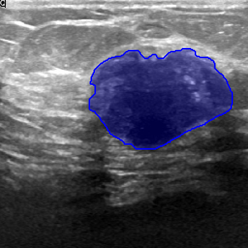
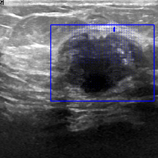
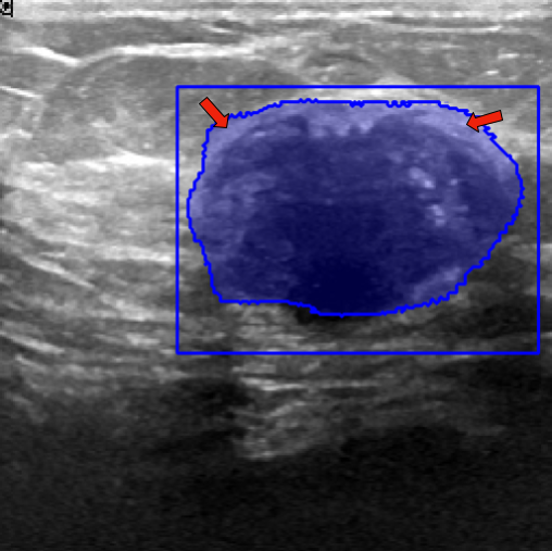
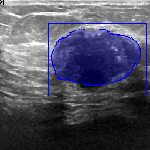
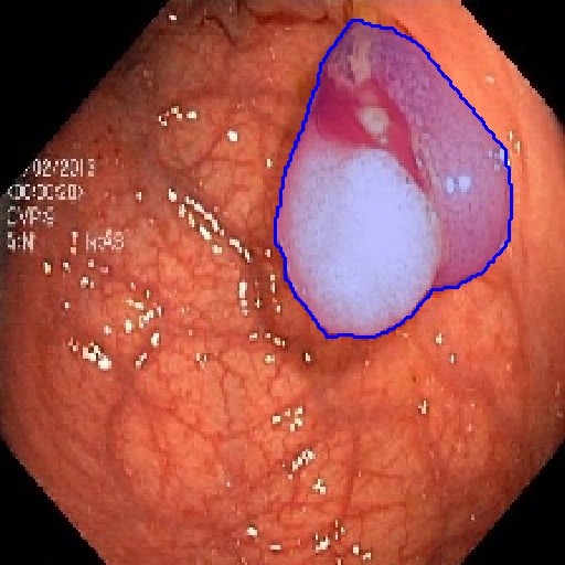
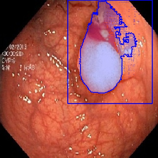
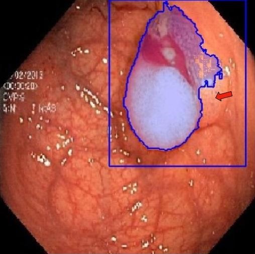
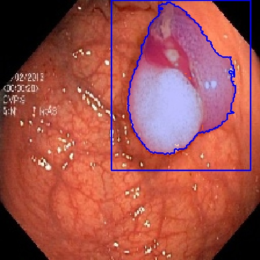
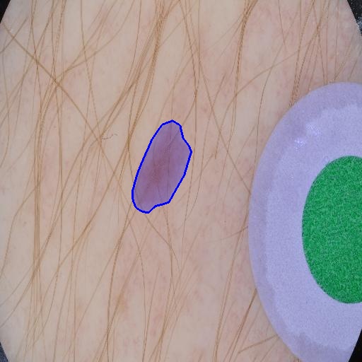
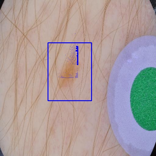
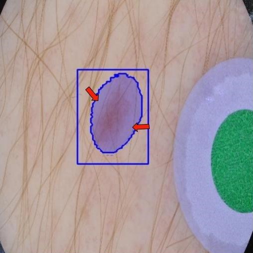
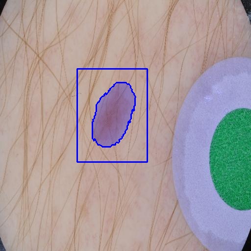
Ground Truth	SAM (no fine-tuning) [6]	SAM (fine-tuning) [9]	LVM-Med (SAM’s ViT)

Figure 7: Visualizing prompt-based predictions on three datasets: BUID, Kvasir, and ISIC. Red arrows show differences between SAM (fine-tuning) and LVM-Med using SAM’s ViT architecture. Best viewed in color with zoom.

Appendix F Dataset overviews

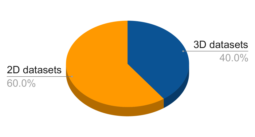
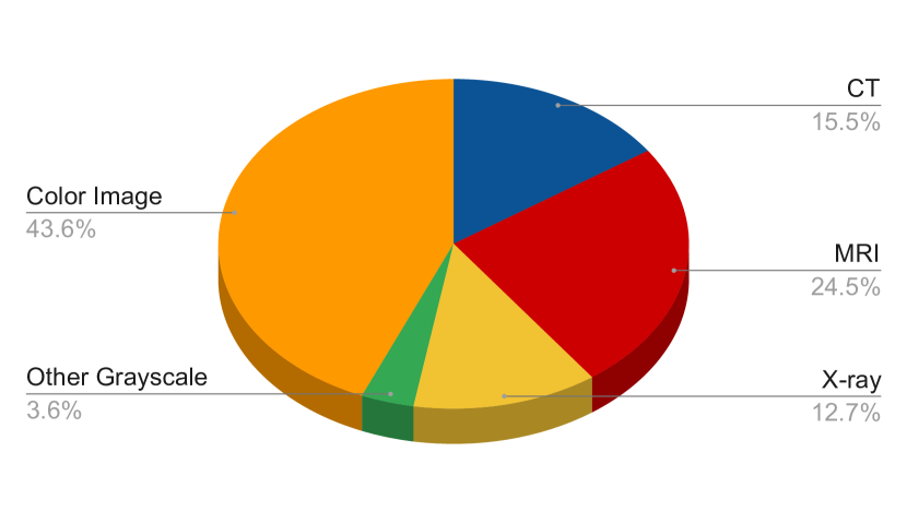
Table 13 overviews the dataset used in our study. For each dataset, we provide its modality, data dimension, and the total of samples. If the training/testing rate is available (column Train/Test Rate), we utilize all training data; otherwise, we sample $20\%$ total samples to avoid potential test data leaking for downstream tasks used in the pre-training step. For datasets whose data dimensions are 3D volumes, we sample 2D slices from those formats. Some datasets, such as MSD or ADNI, comprise different sub-datasets inside; we consider these sub-sets as independent ones to avoid confusion during the training steps. In summary, a total of $55$ datasets are used with approximately $40\%$ in 3D datasets and $60\%$ in 2D images as presented in Figure 8. Moreover, we also outline ratios between distinct data modalities such as MRI, CT, X-ray, grayscale types such as Ultrasound, OCT, and finally, color images depicted in Figure 9. Figure 8: Pie chart illustrating the ratio of the number of datasets with the 3D and 2D dimension. Figure 9: Pie chart illustrating the ratio of different data modalities in our collected dataset.

Table 13: Overview of our collected medical dataset

No	Data Name	Topic	Disease	Modality	Dimension	Train/Test Rate?	Total
1	HyperKvasir [97]	Polyp	Pathological classification	Color images	2D	Yes	110079
2	PatchCamelyon [98, 99]	Cells	Histopathologic scans of lymph node sections.	Color images	2D	Yes	327680
3	BraTS2018 [100, 101, 64]	Brain	Tumor Segmentation	MRI	3D	No	760
4	HNSCC [102]	Head Neck	No Label	CT	3D	No	155
5	LiTS2017 [103]	Liver	Segmentation of Liver and Tumor Lesions	CT	3D	No	200
6	MSD-Heart [96]	Heart	Heart Segmentation	MRI	3D	No	30
7	MSD-Liver [96]	Liver	Liver Segmentation	MRI	3D	No	201
8	MSD-Lung [96]	Lung	Lung Segmentation	MRI	3D	No	96
9	MSD-Pancreas [96]	Pancreas	Pancrea Segmentation	MRI	3D	No	420
10	MSD-HepaticVessel [96]	Hepatic Vessel	Hepatic Vessel Segmentation	MRI	3D	No	443
11	MSD-Spleen [96]	Spleen	Spleen Segmentation	MRI	3D	No	61
12	MSD-Colon [96]	Colon	Colon Segmentation	MRI	3D	No	190
13	OPC-Radiomics [104, 105, 106]	Oropharynx	No Label	CT	3D	No	120
14	Osteosarcoma-UT [107, 108, 105]	Osteosarcoma	No Label	Color images	2D	No	547
15	Pancreas-CT [109, 110, 105]	Pancreas	No Label	CT	3D	No	16

No	Data Name	Topic	Disease	Modality	Format	Default Train/Test Rate	Total
16	Pelvic-Reference-Data [108, 105]	Pelvic	No Label	CT	3D	No	12
17	ProstateX [111, 112, 105]	Prostate	The clinical significance of prostate lesions prediction	MRI	3D	No	40
18	TCGA-CESC [113, 105]	Cervical	No Label	Color images	2D	No	3977
19	TCGA-COAD [114, 105]	Colon	No Label	Color images	2D	No	1644
20	TCGA-ESCA [115, 105]	Cuticle	No Label	Color images	2D	No	4427
21	TCGA-KICH [116, 105]	Kidney	No Label	Color images	2D	No	2192
22	TCGA-KIRC [117, 105]	Kidney	No Label	Color images	2D	No	34108
23	TCGA-READ [114, 105]	Rectum	No Label	Color images	2D	No	248
24	TCGA-SARC [118, 105]	Sarcoma	No Label	Color images	2D	No	624
25	TCGA-THCA [114, 105]	Thyroid	No Label	Color images	2D	No	665
26	VinDr [73]	Lung	Abnormal Disease Classification	X-ray	2D	No	18000
27	LUNA2016 [94]	Lung	Nodule Detection and False Positive Reduction	CT	3D	No	49386
28	BCCD [119]	Cells	Blood cell detection	Color images	2D	No	364
29	C-NMC_Leukemia [120, 121]	Cells	Leukemia detection	Color images	2D	Yes	12529
30	CBIS-DDSM [122, 123]	Breast	Breast Cancer Classification	X-ray	2D	No	6774
31	COVIDx [124]	Lung	Covid-19 Detection	X-ray	2D	Yes	194922
32	Heidelberg OCT [125]	Eye	OCT Imaging Classification	OCT	2D	Yes	84495
33	m2caiSeg [126]	Laparoscopic	Semantic Segmentation Laparoscopic	Color images	2D	Yes	614
34	NuCLS [127]	Nucleus	Nucleus Segmentation Detection / Classification	Color images	2D	Yes	1744
35	SARAS-MESAD [128][129][130]	Prostatectomy Procedures	Action classification in Prostatectomy Surgey	Color images	2D	Yes	29454
36	Shoulder X-ray images from Sun Yat-sen Memorial Hospital [131]	Shoulder	Shoulder X-ray Classification	X-ray	2D	Yes	1049

No	Data Name	Topic	Disease	Modality	Format	Default Train/Test Rate	Total
37	Shenzhen Hospital X-ray Set [132]	Lung	Lung segmentation	X-ray	2D	No	566
38	ADNI 1.5T [133, 134]	Brain	Alzheimer’s Disease Classification	MRI	3D	No	639
39	ADNI 3T [133, 134]	Brain	Alzheimer’s Disease Classification	MRI	3D	No	119
40	AML-Cytomorphology [135, 136, 105]	Cell	Peripheral blood smears	Color images	2D	No	18365
41	APTOS 2019 [137]	Eye	Severity of diabetic retinopathy Classification	Color images	2D	No	3662
42	BCSS [138]	Cells	Breast cancer semantic segmentation	Color images	2D	No	151
43	Dental Panoramic [139]	Tooth	Mandible segmentation	X-ray	2D	No	116
44	HC18 [140]	Fetal	Fetal head circumference (HC)	Ultrasound	2D	No	999
45	Hippseg 2011 [141]	Brain	Hippocampus Segmentation	MRI	3D	No	3050
46	ISIC Challenge 2019 [142]	Skin	Skin Cancer Classification	Color images	2D	No	25331
47	KiTS19-21 [143]	Kidney	Kidney Segmentation	CT	3D	No	45424
48	Kvasir v2 [144]	Gastrointestinal	Gastrointestinal cancer image classification	Color images	2D	No	6000
49	LHNCBC Malaria [145]	Cells	Malaria Classification	Color images	2D	No	27560
50	MitoEM [146]	Cells	Mitochondria Instance Segmentation	MRI/CT	3D	No	1000
51	MLL Bone Marrow [147]	Cells	Blood cell classification	Color images	2D	No	171374
52	MMWHS-CT[65]	Heart	Sub-structure Heart segmentation	CT	3D	Yes	40
53	MMWHS-MRI [65]	Heart	Sub-structure Heart segmentation	MRI	3D	Yes	40
54	RSNA Bone Age [148]	Bone	Bone age prediction	X-ray	2D	No	12611
55	EyePACS [149]	Eye	Diabetic Retinopathy Detection	Color Images	2D	Yes	88702

References

- Cheplygina et al. [2019] Veronika Cheplygina, Marleen de Bruijne, and Josien PW Pluim. Not-so-supervised: a survey of semi-supervised, multi-instance, and transfer learning in medical image analysis. Medical image analysis, 54:280–296, 2019.
- Kaissis et al. [2020] Georgios A Kaissis, Marcus R Makowski, Daniel Rückert, and Rickmer F Braren. Secure, privacy-preserving and federated machine learning in medical imaging. Nature Machine Intelligence, 2(6):305–311, 2020.
- Radford et al. [2021] Alec Radford, Jong Wook Kim, Chris Hallacy, Aditya Ramesh, Gabriel Goh, Sandhini Agarwal, Girish Sastry, Amanda Askell, Pamela Mishkin, Jack Clark, et al. Learning transferable visual models from natural language supervision. In International conference on machine learning, pages 8748–8763. PMLR, 2021.
- Jia et al. [2021] Chao Jia, Yinfei Yang, Ye Xia, Yi-Ting Chen, Zarana Parekh, Hieu Pham, Quoc Le, Yun-Hsuan Sung, Zhen Li, and Tom Duerig. Scaling up visual and vision-language representation learning with noisy text supervision. In International Conference on Machine Learning, pages 4904–4916. PMLR, 2021.
- Singh et al. [2022] Amanpreet Singh, Ronghang Hu, Vedanuj Goswami, Guillaume Couairon, Wojciech Galuba, Marcus Rohrbach, and Douwe Kiela. Flava: A foundational language and vision alignment model. In Proceedings of the IEEE/CVF Conference on Computer Vision and Pattern Recognition, pages 15638–15650, 2022.
- Kirillov et al. [2023a] Alexander Kirillov, Eric Mintun, Nikhila Ravi, Hanzi Mao, Chloe Rolland, Laura Gustafson, Tete Xiao, Spencer Whitehead, Alexander C Berg, Wan-Yen Lo, et al. Segment anything. arXiv preprint arXiv:2304.02643, 2023a.
- Mazurowski et al. [2023] Maciej A Mazurowski, Haoyu Dong, Hanxue Gu, Jichen Yang, Nicholas Konz, and Yixin Zhang. Segment anything model for medical image analysis: an experimental study. arXiv preprint arXiv:2304.10517, 2023.
- He et al. [2023] Sheng He, Rina Bao, Jingpeng Li, P Ellen Grant, and Yangming Ou. Accuracy of segment-anything model (sam) in medical image segmentation tasks. arXiv preprint arXiv:2304.09324, 2023.
- Ma and Wang [2023] Jun Ma and Bo Wang. Segment anything in medical images. arXiv preprint arXiv:2304.12306, 2023.
- Kirillov et al. [2023b] Alexander Kirillov, Eric Mintun, Nikhila Ravi, Hanzi Mao, Chloe Rolland, Laura Gustafson, Tete Xiao, Spencer Whitehead, Alexander C. Berg, Wan-Yen Lo, Piotr Dollár, and Ross Girshick. Segment anything. arXiv:2304.02643, 2023b.
- Sun et al. [2020] Hui Sun, Wenju Zhou, and Minrui Fei. A survey on graph matching in computer vision. In 2020 13th International Congress on Image and Signal Processing, BioMedical Engineering and Informatics (CISP-BMEI), pages 225–230. IEEE, 2020.
- Haller et al. [2022] Stefan Haller, Lorenz Feineis, Lisa Hutschenreiter, Florian Bernard, Carsten Rother, Dagmar Kainmüller, Paul Swoboda, and Bogdan Savchynskyy. A comparative study of graph matching algorithms in computer vision. In Computer Vision–ECCV 2022: 17th European Conference, Tel Aviv, Israel, October 23–27, 2022, Proceedings, Part XXIII, pages 636–653. Springer, 2022.
- Zbontar et al. [2021] Jure Zbontar, Li Jing, Ishan Misra, Yann LeCun, and Stéphane Deny. Barlow twins: Self-supervised learning via redundancy reduction. In International Conference on Machine Learning, pages 12310–12320. PMLR, 2021.
- Bardes et al. [2022] Adrien Bardes, Jean Ponce, and Yann LeCun. Vicregl: Self-supervised learning of local visual features. In NeurIPS, 2022.
- Chen et al. [2020a] Ting Chen, Simon Kornblith, Mohammad Norouzi, and Geoffrey Hinton. A simple framework for contrastive learning of visual representations. In International conference on machine learning, pages 1597–1607. PMLR, 2020a.
- He et al. [2020] Kaiming He, Haoqi Fan, Yuxin Wu, Saining Xie, and Ross Girshick. Momentum contrast for unsupervised visual representation learning. In Proceedings of the IEEE/CVF conference on computer vision and pattern recognition, pages 9729–9738, 2020.
- Chen et al. [2020b] Xinlei Chen, Haoqi Fan, Ross Girshick, and Kaiming He. Improved baselines with momentum contrastive learning. arXiv preprint arXiv:2003.04297, 2020b.
- Tomasev et al. [2022] Nenad Tomasev, Ioana Bica, Brian McWilliams, Lars Buesing, Razvan Pascanu, Charles Blundell, and Jovana Mitrovic. Pushing the limits of self-supervised resnets: Can we outperform supervised learning without labels on imagenet? arXiv preprint arXiv:2201.05119, 2022.
- Tang et al. [2022a] Shixiang Tang, Feng Zhu, Lei Bai, Rui Zhao, Chenyu Wang, and Wanli Ouyang. Unifying visual contrastive learning for object recognition from a graph perspective. In Computer Vision–ECCV 2022: 17th European Conference, Tel Aviv, Israel, October 23–27, 2022, Proceedings, Part XXVI, pages 649–667. Springer, 2022a.
- Caron et al. [2018] Mathilde Caron, Piotr Bojanowski, Armand Joulin, and Matthijs Douze. Deep clustering for unsupervised learning of visual features. In Proceedings of the European conference on computer vision (ECCV), pages 132–149, 2018.
- Caron et al. [2020] Mathilde Caron, Ishan Misra, Julien Mairal, Priya Goyal, Piotr Bojanowski, and Armand Joulin. Unsupervised learning of visual features by contrasting cluster assignments. Advances in neural information processing systems, 33:9912–9924, 2020.
- Zhan et al. [2020] Xiaohang Zhan, Jiahao Xie, Ziwei Liu, Yew-Soon Ong, and Chen Change Loy. Online deep clustering for unsupervised representation learning. In Proceedings of the IEEE/CVF conference on computer vision and pattern recognition, pages 6688–6697, 2020.
- Wu et al. [2018] Zhirong Wu, Yuanjun Xiong, Stella X Yu, and Dahua Lin. Unsupervised feature learning via non-parametric instance discrimination. In Proceedings of the IEEE conference on computer vision and pattern recognition, pages 3733–3742, 2018.
- Chen et al. [2021a] Xinlei Chen, Saining Xie, and Kaiming He. An empirical study of training self-supervised vision transformers. In Proceedings of the IEEE/CVF International Conference on Computer Vision, pages 9640–9649, 2021a.
- Garrido et al. [2022] Quentin Garrido, Yubei Chen, Adrien Bardes, Laurent Najman, and Yann Lecun. On the duality between contrastive and non-contrastive self-supervised learning. arXiv preprint arXiv:2206.02574, 2022.
- Grill et al. [2020] Jean-Bastien Grill, Florian Strub, Florent Altché, Corentin Tallec, Pierre Richemond, Elena Buchatskaya, Carl Doersch, Bernardo Avila Pires, Zhaohan Guo, Mohammad Gheshlaghi Azar, et al. Bootstrap your own latent-a new approach to self-supervised learning. Advances in neural information processing systems, 33:21271–21284, 2020.
- Lee et al. [2021] Kuang-Huei Lee, Anurag Arnab, Sergio Guadarrama, John Canny, and Ian Fischer. Compressive visual representations. Advances in Neural Information Processing Systems, 34:19538–19552, 2021.
- Xiao et al. [2021] Tete Xiao, Colorado J Reed, Xiaolong Wang, Kurt Keutzer, and Trevor Darrell. Region similarity representation learning. In Proceedings of the IEEE/CVF International Conference on Computer Vision, pages 10539–10548, 2021.
- Wang et al. [2021] Xinlong Wang, Rufeng Zhang, Chunhua Shen, Tao Kong, and Lei Li. Dense contrastive learning for self-supervised visual pre-training. In Proceedings of the IEEE/CVF Conference on Computer Vision and Pattern Recognition, pages 3024–3033, 2021.
- Zhuang et al. [2019] Xinrui Zhuang, Yuexiang Li, Yifan Hu, Kai Ma, Yujiu Yang, and Yefeng Zheng. Self-supervised feature learning for 3d medical images by playing a rubik’s cube. In International Conference on Medical Image Computing and Computer-Assisted Intervention, pages 420–428. Springer, 2019.
- Chen et al. [2019a] Liang Chen, Paul Bentley, Kensaku Mori, Kazunari Misawa, Michitaka Fujiwara, and Daniel Rueckert. Self-supervised learning for medical image analysis using image context restoration. Medical image analysis, 58:101539, 2019a.
- Zhou et al. [2021] Zongwei Zhou, Vatsal Sodha, Jiaxuan Pang, Michael B Gotway, and Jianming Liang. Models genesis. Medical image analysis, 67:101840, 2021.
- Haghighi et al. [2021] Fatemeh Haghighi, Mohammad Reza Hosseinzadeh Taher, Zongwei Zhou, Michael B Gotway, and Jianming Liang. Transferable visual words: Exploiting the semantics of anatomical patterns for self-supervised learning. IEEE transactions on medical imaging, 40(10):2857–2868, 2021.
- Bommasani et al. [2021] Rishi Bommasani, Drew A Hudson, Ehsan Adeli, Russ Altman, Simran Arora, Sydney von Arx, Michael S Bernstein, Jeannette Bohg, Antoine Bosselut, Emma Brunskill, et al. On the opportunities and risks of foundation models. arXiv preprint arXiv:2108.07258, 2021.
- Wang et al. [2022] Junke Wang, Dongdong Chen, Zuxuan Wu, Chong Luo, Luowei Zhou, Yucheng Zhao, Yujia Xie, Ce Liu, Yu-Gang Jiang, and Lu Yuan. Omnivl: One foundation model for image-language and video-language tasks. arXiv preprint arXiv:2209.07526, 2022.
- Ma et al. [2021] Jiayi Ma, Xingyu Jiang, Aoxiang Fan, Junjun Jiang, and Junchi Yan. Image matching from handcrafted to deep features: A survey. International Journal of Computer Vision, 129:23–79, 2021.
- Cao and Bernard [2023] Dongliang Cao and Florian Bernard. Self-supervised learning for multimodal non-rigid 3d shape matching. In Proceedings of the IEEE/CVF Conference on Computer Vision and Pattern Recognition, pages 17735–17744, 2023.
- Yilmaz et al. [2006] Alper Yilmaz, Omar Javed, and Mubarak Shah. Object tracking: A survey. Acm computing surveys (CSUR), 38(4):13–es, 2006.
- Hyun et al. [2023] Jeongseok Hyun, Myunggu Kang, Dongyoon Wee, and Dit-Yan Yeung. Detection recovery in online multi-object tracking with sparse graph tracker. In Proceedings of the IEEE/CVF Winter Conference on Applications of Computer Vision, pages 4850–4859, 2023.
- Heimann and Meinzer [2009] Tobias Heimann and Hans-Peter Meinzer. Statistical shape models for 3d medical image segmentation: a review. Medical image analysis, 13(4):543–563, 2009.
- Roetzer et al. [2023] Paul Roetzer, Zorah Lähner, and Florian Bernard. Conjugate product graphs for globally optimal 2d-3d shape matching. In Proceedings of the IEEE/CVF Conference on Computer Vision and Pattern Recognition, pages 21866–21875, 2023.
- Bian et al. [2022] Yikai Bian, Le Hui, Jianjun Qian, and Jin Xie. Unsupervised domain adaptation for point cloud semantic segmentation via graph matching. In 2022 IEEE/RSJ International Conference on Intelligent Robots and Systems (IROS), pages 9899–9904. IEEE, 2022.
- Wu and Ye [2023] Zesen Wu and Mang Ye. Unsupervised visible-infrared person re-identification via progressive graph matching and alternate learning. In Proceedings of the IEEE/CVF Conference on Computer Vision and Pattern Recognition, pages 9548–9558, 2023.
- Peng et al. [2022] Liang Peng, Nan Wang, Jie Xu, Xiaofeng Zhu, and Xiaoxiao Li. Gate: graph cca for temporal self-supervised learning for label-efficient fmri analysis. IEEE Transactions on Medical Imaging, 42(2):391–402, 2022.
- Liu et al. [2022] Chang Liu, Shaofeng Zhang, Xiaokang Yang, and Junchi Yan. Self-supervised learning of visual graph matching. In European Conference on Computer Vision, pages 370–388. Springer, 2022.
- Zass and Shashua [2008] Ron Zass and Amnon Shashua. Probabilistic graph and hypergraph matching. In 2008 IEEE Conference on Computer Vision and Pattern Recognition, pages 1–8. IEEE, 2008.
- Zhou and De la Torre [2015] Feng Zhou and Fernando De la Torre. Factorized graph matching. IEEE transactions on pattern analysis and machine intelligence, 38(9):1774–1789, 2015.
- Pogančić et al. [2020] Marin Vlastelica Pogančić, Anselm Paulus, Vit Musil, Georg Martius, and Michal Rolinek. Differentiation of blackbox combinatorial solvers. In International Conference on Learning Representations, 2020.
- Rolínek et al. [2020a] Michal Rolínek, Paul Swoboda, Dominik Zietlow, Anselm Paulus, Vít Musil, and Georg Martius. Deep graph matching via blackbox differentiation of combinatorial solvers. In Computer Vision–ECCV 2020: 16th European Conference, Glasgow, UK, August 23–28, 2020, Proceedings, Part XXVIII 16, pages 407–424. Springer, 2020a.
- Niepert et al. [2021] Mathias Niepert, Pasquale Minervini, and Luca Franceschi. Implicit MLE: backpropagating through discrete exponential family distributions. In NeurIPS, Proceedings of Machine Learning Research. PMLR, 2021.
- Kipf and Welling [2017] Thomas N. Kipf and Max Welling. Semi-supervised classification with graph convolutional networks. In 5th International Conference on Learning Representations, ICLR 2017, Toulon, France, April 24-26, 2017, Conference Track Proceedings. OpenReview.net, 2017. URL https://openreview.net/forum?id=SJU4ayYgl.
- Wu et al. [2019] Felix Wu, Amauri Souza, Tianyi Zhang, Christopher Fifty, Tao Yu, and Kilian Weinberger. Simplifying graph convolutional networks. In International conference on machine learning, pages 6861–6871. PMLR, 2019.
- Yang et al. [2022] Junwei Yang, Ke Zhang, Zhaolin Cui, Jinming Su, Junfeng Luo, and Xiaolin Wei. Inscon: instance consistency feature representation via self-supervised learning. arXiv preprint arXiv:2203.07688, 2022.
- Xie et al. [2021] Zhenda Xie, Yutong Lin, Zheng Zhang, Yue Cao, Stephen Lin, and Han Hu. Propagate yourself: Exploring pixel-level consistency for unsupervised visual representation learning. In Proceedings of the IEEE/CVF Conference on Computer Vision and Pattern Recognition, pages 16684–16693, 2021.
- Burkard et al. [1998] Rainer E Burkard, Eranda Cela, Panos M Pardalos, and Leonidas S Pitsoulis. The quadratic assignment problem. Springer, 1998.
- Swoboda et al. [2017] Paul Swoboda, Carsten Rother, Hassan Abu Alhaija, Dagmar Kainmuller, and Bogdan Savchynskyy. A study of lagrangean decompositions and dual ascent solvers for graph matching. In Proceedings of the IEEE conference on computer vision and pattern recognition, pages 1607–1616, 2017.
- Rolínek et al. [2020b] Michal Rolínek, Vít Musil, Anselm Paulus, Marin Vlastelica, Claudio Michaelis, and Georg Martius. Optimizing rank-based metrics with blackbox differentiation. In Proceedings of the IEEE/CVF Conference on Computer Vision and Pattern Recognition, pages 7620–7630, 2020b.
- Minervini et al. [2022] Pasquale Minervini, Luca Franceschi, and Mathias Niepert. Adaptive perturbation-based gradient estimation for discrete latent variable models. arXiv preprint arXiv:2209.04862, 2022.
- Papandreou and Yuille [2011] George Papandreou and Alan L Yuille. Perturb-and-map random fields: Using discrete optimization to learn and sample from energy models. In 2011 International Conference on Computer Vision, pages 193–200. IEEE, 2011.
- He et al. [2016] Kaiming He, Xiangyu Zhang, Shaoqing Ren, and Jian Sun. Deep residual learning for image recognition. In Proceedings of the IEEE conference on computer vision and pattern recognition, pages 770–778, 2016.
- Dosovitskiy et al. [2020] Alexey Dosovitskiy, Lucas Beyer, Alexander Kolesnikov, Dirk Weissenborn, Xiaohua Zhai, Thomas Unterthiner, Mostafa Dehghani, Matthias Minderer, Georg Heigold, Sylvain Gelly, et al. An image is worth 16x16 words: Transformers for image recognition at scale. arXiv preprint arXiv:2010.11929, 2020.
- Deng et al. [2009] Jia Deng, Wei Dong, Richard Socher, Li-Jia Li, Kai Li, and Li Fei-Fei. Imagenet: A large-scale hierarchical image database. In 2009 IEEE conference on computer vision and pattern recognition, pages 248–255. Ieee, 2009.
- Kingma and Ba [2014] Diederik P Kingma and Jimmy Ba. Adam: A method for stochastic optimization. arXiv preprint arXiv:1412.6980, 2014.
- Bakas et al. [2018] Spyridon Bakas, Mauricio Reyes, Andras Jakab, Stefan Bauer, Markus Rempfler, Alessandro Crimi, Russell Takeshi Shinohara, Christoph Berger, Sung Min Ha, Martin Rozycki, et al. Identifying the best machine learning algorithms for brain tumor segmentation, progression assessment, and overall survival prediction in the brats challenge. arXiv preprint arXiv:1811.02629, 2018.
- Zhuang and Shen [2016] Xiahai Zhuang and Juan Shen. Multi-scale patch and multi-modality atlases for whole heart segmentation of mri. Medical image analysis, 31:77–87, 2016.
- Codella et al. [2019] Noel Codella, Veronica Rotemberg, Philipp Tschandl, M Emre Celebi, Stephen Dusza, David Gutman, Brian Helba, Aadi Kalloo, Konstantinos Liopyris, Michael Marchetti, et al. Skin lesion analysis toward melanoma detection 2018: A challenge hosted by the international skin imaging collaboration (isic). arXiv preprint arXiv:1902.03368, 2019.
- Shiraishi et al. [2000] Junji Shiraishi, Shigehiko Katsuragawa, Junpei Ikezoe, Tsuneo Matsumoto, Takeshi Kobayashi, Ken-ichi Komatsu, Mitate Matsui, Hiroshi Fujita, Yoshie Kodera, and Kunio Doi. Development of a digital image database for chest radiographs with and without a lung nodule: receiver operating characteristic analysis of radiologists’ detection of pulmonary nodules. American Journal of Roentgenology, 174(1):71–74, 2000.
- Pogorelov et al. [2017] Konstantin Pogorelov, Kristin Ranheim Randel, Carsten Griwodz, Sigrun Losada Eskeland, Thomas de Lange, Dag Johansen, Concetto Spampinato, Duc-Tien Dang-Nguyen, Mathias Lux, Peter Thelin Schmidt, et al. Kvasir: A multi-class image dataset for computer aided gastrointestinal disease detection. In Proceedings of the 8th ACM on Multimedia Systems Conference, pages 164–169, 2017.
- Staal et al. [2004] Joes Staal, Michael D Abràmoff, Meindert Niemeijer, Max A Viergever, and Bram Van Ginneken. Ridge-based vessel segmentation in color images of the retina. IEEE transactions on medical imaging, 23(4):501–509, 2004.
- Al-Dhabyani et al. [2020] Walid Al-Dhabyani, Mohammed Gomaa, Hussien Khaled, and Aly Fahmy. Dataset of breast ultrasound images. Data in brief, 28:104863, 2020.
- Zhou et al. [2020] Yi Zhou, Boyang Wang, Lei Huang, Shanshan Cui, and Ling Shao. A benchmark for studying diabetic retinopathy: segmentation, grading, and transferability. IEEE Transactions on Medical Imaging, 40(3):818–828, 2020.
- Liu et al. [2020] Quande Liu, Qi Dou, Lequan Yu, and Pheng Ann Heng. Ms-net: Multi-site network for improving prostate segmentation with heterogeneous mri data. IEEE Transactions on Medical Imaging, 2020.
- Nguyen et al. [2022a] Ha Q Nguyen, Khanh Lam, Linh T Le, Hieu H Pham, Dat Q Tran, Dung B Nguyen, Dung D Le, Chi M Pham, Hang TT Tong, Diep H Dinh, et al. Vindr-cxr: An open dataset of chest x-rays with radiologist’s annotations. Scientific Data, 9(1):429, 2022a.
- Kamran et al. [2021] Sharif Amit Kamran, Khondker Fariha Hossain, Alireza Tavakkoli, Stewart Lee Zuckerbrod, Kenton M Sanders, and Salah A Baker. Rv-gan: Segmenting retinal vascular structure in fundus photographs using a novel multi-scale generative adversarial network. In Medical Image Computing and Computer Assisted Intervention–MICCAI 2021: 24th International Conference, Strasbourg, France, September 27–October 1, 2021, Proceedings, Part VIII 24, pages 34–44. Springer, 2021.
- Myronenko [2019] Andriy Myronenko. 3d mri brain tumor segmentation using autoencoder regularization. In Brainlesion: Glioma, Multiple Sclerosis, Stroke and Traumatic Brain Injuries: 4th International Workshop, BrainLes 2018, Held in Conjunction with MICCAI 2018, Granada, Spain, September 16, 2018, Revised Selected Papers, Part II 4, pages 311–320. Springer, 2019.
- Chen et al. [2021b] Jieneng Chen, Yongyi Lu, Qihang Yu, Xiangde Luo, Ehsan Adeli, Yan Wang, Le Lu, Alan L Yuille, and Yuyin Zhou. Transunet: Transformers make strong encoders for medical image segmentation. arXiv preprint arXiv:2102.04306, 2021b.
- Oktay et al. [2018] Ozan Oktay, Jo Schlemper, Loic Le Folgoc, Matthew Lee, Mattias Heinrich, Kazunari Misawa, Kensaku Mori, Steven McDonagh, Nils Y Hammerla, Bernhard Kainz, et al. Attention u-net: Learning where to look for the pancreas. arXiv preprint arXiv:1804.03999, 2018.
- Zhou et al. [2018] Z Zhou, MMR Siddiquee, N Tajbakhsh, and J UNet+ Liang. A nested u-net architecture for medical image segmentation (2018). arXiv preprint arXiv:1807.10165, 2018.
- Caron et al. [2021] Mathilde Caron, Hugo Touvron, Ishan Misra, Hervé Jégou, Julien Mairal, Piotr Bojanowski, and Armand Joulin. Emerging properties in self-supervised vision transformers. In Proceedings of the IEEE/CVF international conference on computer vision, pages 9650–9660, 2021.
- Hatamizadeh et al. [2022] Ali Hatamizadeh, Yucheng Tang, Vishwesh Nath, Dong Yang, Andriy Myronenko, Bennett Landman, Holger R Roth, and Daguang Xu. Unetr: Transformers for 3d medical image segmentation. In Proceedings of the IEEE/CVF Winter Conference on Applications of Computer Vision, pages 574–584, 2022.
- Carreira and Zisserman [2017] Joao Carreira and Andrew Zisserman. Quo vadis, action recognition? a new model and the kinetics dataset. In proceedings of the IEEE Conference on Computer Vision and Pattern Recognition, pages 6299–6308, 2017.
- Gibson et al. [2018] Eli Gibson, Wenqi Li, Carole Sudre, Lucas Fidon, Dzhoshkun I Shakir, Guotai Wang, Zach Eaton-Rosen, Robert Gray, Tom Doel, Yipeng Hu, et al. NiftyNet: a deep-learning platform for medical imaging. Computer methods and programs in biomedicine, 158:113–122, 2018.
- Chen et al. [2019b] Sihong Chen, Kai Ma, and Yefeng Zheng. Med3d: Transfer learning for 3d medical image analysis. arXiv:1904.00625, 2019b.
- Zhang et al. [2020] Xiaoman Zhang, Ya Zhang, Xiaoyun Zhang, and Yanfeng Wang. Universal model for 3d medical image analysis. ArXiv, abs/2010.06107, 2020.
- Tang et al. [2022b] Yucheng Tang, Dong Yang, Wenqi Li, Holger R Roth, Bennett Landman, Daguang Xu, Vishwesh Nath, and Ali Hatamizadeh. Self-supervised pre-training of swin transformers for 3d medical image analysis. In Proceedings of the IEEE/CVF Conference on Computer Vision and Pattern Recognition, pages 20730–20740, 2022b.
- Nguyen et al. [2022b] Duy MH Nguyen, Hoang Nguyen, Mai TN Truong, Tri Cao, Binh T Nguyen, Nhat Ho, Paul Swoboda, Shadi Albarqouni, Pengtao Xie, and Daniel Sonntag. Joint self-supervised image-volume representation learning with intra-inter contrastive clustering. arXiv preprint arXiv:2212.01893, 2022b.
- Lin et al. [2018] Zhiwen Lin, Ruoqian Guo, Yanjie Wang, Bian Wu, Tingting Chen, Wenzhe Wang, Danny Z Chen, and Jian Wu. A framework for identifying diabetic retinopathy based on anti-noise detection and attention-based fusion. In Medical Image Computing and Computer Assisted Intervention–MICCAI 2018: 21st International Conference, Granada, Spain, September 16-20, 2018, Proceedings, Part II 11, pages 74–82. Springer, 2018.
- Wu et al. [2021] Yu-Huan Wu, Shang-Hua Gao, Jie Mei, Jun Xu, Deng-Ping Fan, Rong-Guo Zhang, and Ming-Ming Cheng. Jcs: An explainable covid-19 diagnosis system by joint classification and segmentation. IEEE Transactions on Image Processing, 30:3113–3126, 2021.
- Zhou et al. [2019] Yi Zhou, Xiaodong He, Lei Huang, Li Liu, Fan Zhu, Shanshan Cui, and Ling Shao. Collaborative learning of semi-supervised segmentation and classification for medical images. In Proceedings of the IEEE/CVF conference on computer vision and pattern recognition, pages 2079–2088, 2019.
- Tusfiqur et al. [2022] Hasan Md Tusfiqur, Duy MH Nguyen, Mai TN Truong, Triet A Nguyen, Binh T Nguyen, Michael Barz, Hans-Juergen Profitlich, Ngoc TT Than, Ngan Le, Pengtao Xie, et al. Drg-net: Interactive joint learning of multi-lesion segmentation and classification for diabetic retinopathy grading. arXiv preprint arXiv:2212.14615, 2022.
- Ronneberger et al. [2015] Olaf Ronneberger, Philipp Fischer, and Thomas Brox. U-net: Convolutional networks for biomedical image segmentation. In Medical Image Computing and Computer-Assisted Intervention–MICCAI 2015: 18th International Conference, Munich, Germany, October 5-9, 2015, Proceedings, Part III 18, pages 234–241. Springer, 2015.
- Jadon [2020] Shruti Jadon. A survey of loss functions for semantic segmentation. In 2020 IEEE conference on computational intelligence in bioinformatics and computational biology (CIBCB), pages 1–7. IEEE, 2020.
- Girshick [2015] Ross Girshick. Fast r-cnn. In Proceedings of the IEEE international conference on computer vision, pages 1440–1448, 2015.
- Setio et al. [2015] Arnaud AA Setio, Colin Jacobs, Jaap Gelderblom, and Bram van Ginneken. Automatic detection of large pulmonary solid nodules in thoracic ct images. Medical physics, 42(10):5642–5653, 2015.
- Bilic et al. [2019] Patrick Bilic, Patrick Ferdinand Christ, Eugene Vorontsov, Grzegorz Chlebus, Hao Chen, Qi Dou, Chi-Wing Fu, Xiao Han, Pheng-Ann Heng, Jürgen Hesser, et al. The liver tumor segmentation benchmark (LiTS). arXiv:1901.04056, 2019.
- Simpson et al. [2019] Amber L Simpson, Michela Antonelli, Spyridon Bakas, Michel Bilello, Keyvan Farahani, Bram Van Ginneken, Annette Kopp-Schneider, Bennett A Landman, Geert Litjens, Bjoern Menze, et al. A large annotated medical image dataset for the development and evaluation of segmentation algorithms. arXiv preprint arXiv:1902.09063, 2019.
- Borgli et al. [2020] Hanna Borgli, Vajira Thambawita, Pia H Smedsrud, Steven Hicks, Debesh Jha, Sigrun L Eskeland, Kristin Ranheim Randel, Konstantin Pogorelov, Mathias Lux, Duc Tien Dang Nguyen, et al. Hyperkvasir, a comprehensive multi-class image and video dataset for gastrointestinal endoscopy. Scientific data, 7(1):283, 2020.
- Veeling et al. [2018] Bastiaan S Veeling, Jasper Linmans, Jim Winkens, Taco Cohen, and Max Welling. Rotation equivariant CNNs for digital pathology. June 2018.
- Bejnordi et al. [2017] Babak Ehteshami Bejnordi, Mitko Veta, Paul Johannes Van Diest, Bram Van Ginneken, Nico Karssemeijer, Geert Litjens, Jeroen AWM Van Der Laak, Meyke Hermsen, Quirine F Manson, Maschenka Balkenhol, et al. Diagnostic assessment of deep learning algorithms for detection of lymph node metastases in women with breast cancer. Jama, 318(22):2199–2210, 2017.
- Menze et al. [2015] Bjoern H. Menze, Andras Jakab, Stefan Bauer, Jayashree Kalpathy-Cramer, Keyvan Farahani, Justin Kirby, Yuliya Burren, Nicole Porz, Johannes Slotboom, Roland Wiest, Levente Lanczi, Elizabeth Gerstner, Marc-André Weber, Tal Arbel, Brian B. Avants, Nicholas Ayache, Patricia Buendia, D. Louis Collins, Nicolas Cordier, Jason J. Corso, Antonio Criminisi, Tilak Das, Hervé Delingette, Çağatay Demiralp, Christopher R. Durst, Michel Dojat, Senan Doyle, Joana Festa, Florence Forbes, Ezequiel Geremia, Ben Glocker, Polina Golland, Xiaotao Guo, Andac Hamamci, Khan M. Iftekharuddin, Raj Jena, Nigel M. John, Ender Konukoglu, Danial Lashkari, José António Mariz, Raphael Meier, Sérgio Pereira, Doina Precup, Stephen J. Price, Tammy Riklin Raviv, Syed M. S. Reza, Michael Ryan, Duygu Sarikaya, Lawrence Schwartz, Hoo-Chang Shin, Jamie Shotton, Carlos A. Silva, Nuno Sousa, Nagesh K. Subbanna, Gabor Szekely, Thomas J. Taylor, Owen M. Thomas, Nicholas J. Tustison, Gozde Unal, Flor Vasseur, Max Wintermark, Dong Hye Ye, Liang Zhao, Binsheng Zhao, Darko Zikic, Marcel Prastawa, Mauricio Reyes, and Koen Van Leemput. The multimodal brain tumor image segmentation benchmark (brats). IEEE Transactions on Medical Imaging, 34(10):1993–2024, 2015. doi: 10.1109/TMI.2014.2377694.
- Lloyd et al. [2017] Christopher T Lloyd, Alessandro Sorichetta, and Andrew J Tatem. High resolution global gridded data for use in population studies. Scientific data, 4(1):1–17, 2017.
- Grossberg et al. [2018] Aaron J Grossberg, Abdallah SR Mohamed, Hesham Elhalawani, William C Bennett, Kirk E Smith, Tracy S Nolan, Bowman Williams, Sasikarn Chamchod, Jolien Heukelom, Michael E Kantor, et al. Imaging and clinical data archive for head and neck squamous cell carcinoma patients treated with radiotherapy. Scientific data, 5(1):1–10, 2018.
- Bilic et al. [2023] Patrick Bilic, Patrick Christ, Hongwei Bran Li, Eugene Vorontsov, Avi Ben-Cohen, Georgios Kaissis, Adi Szeskin, Colin Jacobs, Gabriel Efrain Humpire Mamani, Gabriel Chartrand, et al. The liver tumor segmentation benchmark (lits). Medical Image Analysis, 84:102680, 2023.
- Kwan et al. [2018] Jennifer Yin Yee Kwan, Jie Su, Shao Hui Huang, Laleh S Ghoraie, Wei Xu, Biu Chan, Kenneth W Yip, Meredith Giuliani, Andrew Bayley, John Kim, et al. Radiomic biomarkers to refine risk models for distant metastasis in hpv-related oropharyngeal carcinoma. International Journal of Radiation Oncology* Biology* Physics, 102(4):1107–1116, 2018.
- Clark et al. [2013] Kenneth Clark, Bruce Vendt, Kirk Smith, John Freymann, Justin Kirby, Paul Koppel, Stephen Moore, Stanley Phillips, David Maffitt, Michael Pringle, et al. The cancer imaging archive (tcia): maintaining and operating a public information repository. Journal of digital imaging, 26:1045–1057, 2013.
- [106] JYY Kwan et al. Data from radiomic biomarkers to refine risk models for distant metastasis in oropharyngeal carcinoma, the cancer imaging archive, 2019.
- Leavey et al. [2019] P Leavey, A Sengupta, D Rakheja, O Daescu, HB Arunachalam, and R Mishra. Osteosarcoma data from ut southwestern/ut dallas for viable and necrotic tumor assessment [data set]. The Cancer Imaging Archive, 14, 2019.
- Yorke et al. [2019] AA Yorke, GC McDonald, D Solis, and T Guerrero. Pelvic reference data. Cancer Imaging Arch, 2019.
- Roth et al. [2016] Holger R Roth, Amal Farag, E Turkbey, Le Lu, Jiamin Liu, and Ronald M Summers. Data from pancreas-ct. the cancer imaging archive. IEEE Transactions on Image Processing, 2016.
- Roth et al. [2015] Holger R Roth, Le Lu, Amal Farag, Hoo-Chang Shin, Jiamin Liu, Evrim B Turkbey, and Ronald M Summers. Deeporgan: Multi-level deep convolutional networks for automated pancreas segmentation. In Medical Image Computing and Computer-Assisted Intervention–MICCAI 2015: 18th International Conference, Munich, Germany, October 5-9, 2015, Proceedings, Part I 18, pages 556–564. Springer, 2015.
- Litjens et al. [2014] Geert Litjens, Oscar Debats, Jelle Barentsz, Nico Karssemeijer, and Henkjan Huisman. Computer-aided detection of prostate cancer in mri. IEEE transactions on medical imaging, 33(5):1083–1092, 2014.
- Litjens et al. [2017] Geert Litjens, Oscar Debats, Jelle Barentsz, Nico Karssemeijer, and Henkjan Huisman. Prostatex challenge data. The Cancer Imaging Archive, 2017. https://doi.org/10.7937/K9/TCIA.2017.SMPYMRXQ.
- Lucchesi and Aredes [2016a] FR Lucchesi and ND Aredes. Radiology data from the cancer genome atlas cervical squamous cell carcinoma and endocervical adenocarcinoma (tcga-cesc) collection. the cancer imaging archive. Cancer Imaging Arch, 2016a.
- Kirk et al. [2016] S Kirk, Y Lee, CA Sadow, S Levine, C Roche, E Bonaccio, and J Filiippini. Radiology data from the cancer genome atlas colon adenocarcinoma [tcga-coad] collection. The Cancer Imaging Archive, 2016.
- Lucchesi and Aredes [2016b] F. R. Lucchesi and N. D. Aredes. The cancer genome atlas esophageal carcinoma collection (tcga-esca) (version 3) [data set]. The Cancer Imaging Archive, 2016b.
- Linehan et al. [2016] MW Linehan, R Gautam, CA Sadow, and S Levine. Radiology data from the cancer genome atlas kidney chromophobe [tcga-kich] collection. The Cancer Imaging Archive, 2016.
- Akin et al. [2016] O Akin, P Elnajjar, M Heller, R Jarosz, B Erickson, S Kirk, and J Filippini. Radiology data from the cancer genome atlas kidney renal clear cell carcinoma [tcga-kirc] collection. The Cancer Imaging Archive, 1310, 2016.
- Roche et al. [2016] C Roche, E Bonaccio, and J Filippini. Radiology data from the cancer genome atlas sarcoma [tcga-sarc] collection. Cancer Imaging Arch. https://doi. org/10.7937 K, 9, 2016.
- Shenggan [2017] Shenggan. Bccd dataset, 2017. URL https://github.com/Shenggan/BCCD_Dataset.
- Gehlot et al. [2020] Shiv Gehlot, Anubha Gupta, and Ritu Gupta. Sdct-auxnet: Dct augmented stain deconvolutional cnn with auxiliary classifier for cancer diagnosis. Medical image analysis, 61:101661, 2020.
- Gupta and Gupta [2019] A Gupta and R Gupta. All challenge dataset of isbi 2019 [data set]. URL https://doi.org/10.7937/tcia.2019.dc64i46r, 2019.
- Lee et al. [2017] Rebecca Sawyer Lee, Francisco Gimenez, Assaf Hoogi, Kanae Kawai Miyake, Mia Gorovoy, and Daniel L Rubin. A curated mammography data set for use in computer-aided detection and diagnosis research. Scientific data, 4(1):1–9, 2017.
- Sawyer Lee et al. [2016] R Sawyer Lee, F Gimenez, A Hoogi, and D Rubin. Curated breast imaging subset of ddsm. The Cancer Imaging Archive. DOI: https://doi. org/10.7937 K, 9, 2016.
- Wang et al. [2020] Linda Wang, Zhong Qiu Lin, and Alexander Wong. Covid-net: a tailored deep convolutional neural network design for detection of covid-19 cases from chest x-ray images. Scientific Reports, 10(1):19549, Nov 2020. ISSN 2045-2322. doi: 10.1038/s41598-020-76550-z. URL https://doi.org/10.1038/s41598-020-76550-z.
- Kermany et al. [2018] Daniel Kermany, Kang Zhang, Michael Goldbaum, et al. Labeled optical coherence tomography (oct) and chest x-ray images for classification. Mendeley data, 2(2):651, 2018.
- Maqbool et al. [2020] Salman Maqbool, Aqsa Riaz, Hasan Sajid, and Osman Hasan. m2caiseg: Semantic segmentation of laparoscopic images using convolutional neural networks. arXiv preprint arXiv:2008.10134, 2020.
- Amgad et al. [2019a] Mohamed Amgad, Habiba Elfandy, Hagar Hussein, Lamees A Atteya, Mai A T Elsebaie, Lamia S Abo Elnasr, Rokia A Sakr, Hazem S E Salem, Ahmed F Ismail, Anas M Saad, Joumana Ahmed, Maha A T Elsebaie, Mustafijur Rahman, Inas A Ruhban, Nada M Elgazar, Yahya Alagha, Mohamed H Osman, Ahmed M Alhusseiny, Mariam M Khalaf, Abo-Alela F Younes, Ali Abdulkarim, Duaa M Younes, Ahmed M Gadallah, Ahmad M Elkashash, Salma Y Fala, Basma M Zaki, Jonathan Beezley, Deepak R Chittajallu, David Manthey, David A Gutman, and Lee A D Cooper. Structured crowdsourcing enables convolutional segmentation of histology images. Bioinformatics, 35(18):3461–3467, 02 2019a. ISSN 1367-4803. doi: 10.1093/bioinformatics/btz083. URL https://doi.org/10.1093/bioinformatics/btz083.
- Cuzzolin et al. [2021] Fabio Cuzzolin, Vivek Singh Bawa, Inna Skarga-Bandurova, Mohamed Mohamed, Jackson Ravindran Charles, Elettra Oleari, Alice Leporini, Carmela Landolfo, Armando Stabile, Francesco Setti, et al. Saras challenge on multi-domain endoscopic surgeon action detection, 2021.
- Bawa et al. [2021] Vivek Singh Bawa, Gurkirt Singh, Francis KapingA, Inna Skarga-Bandurova, Elettra Oleari, Alice Leporini, Carmela Landolfo, Pengfei Zhao, Xi Xiang, Gongning Luo, Kuanquan Wang, Liangzhi Li, Bowen Wang, Shang Zhao, Li Li, Armando Stabile, Francesco Setti, Riccardo Muradore, and Fabio Cuzzolin. The saras endoscopic surgeon action detection (esad) dataset: Challenges and methods, 2021.
- Bawa et al. [2020] Vivek Singh Bawa, Gurkirt Singh, Francis KapingA, Inna Skarga-Bandurova, Alice Leporini, Carmela Landolfo, Armando Stabile, Francesco Setti, Riccardo Muradore, Elettra Oleari, and Fabio Cuzzolin. Esad: Endoscopic surgeon action detection dataset, 2020.
- [131] Shoulder x-ray classification. Kaggle dataset. URL https://www.kaggle.com/datasets/dryari5/shoulder-xray-classification.
- [132] Lung masks for shenzhen hospital chest x-ray set. Kaggle dataset. URL https://www.kaggle.com/datasets/yoctoman/shcxr-lung-mask.
- Mueller et al. [2005] Susanne G Mueller, Michael W Weiner, Leon J Thal, Ronald C Petersen, Clifford Jack, William Jagust, John Q Trojanowski, Arthur W Toga, and Laurel Beckett. The alzheimer’s disease neuroimaging initiative. Neuroimaging Clinics, 15(4):869–877, 2005.
- Petersen et al. [2010] Ronald Carl Petersen, Paul S Aisen, Laurel A Beckett, Michael C Donohue, Anthony Collins Gamst, Danielle J Harvey, Clifford R Jack, William J Jagust, Leslie M Shaw, Arthur W Toga, et al. Alzheimer’s disease neuroimaging initiative (adni): clinical characterization. Neurology, 74(3):201–209, 2010.
- Matek et al. [2019a] Christian Matek, Simone Schwarz, Carsten Marr, and Karsten Spiekermann. A single-cell morphological dataset of leukocytes from aml patients and non-malignant controls (aml-cytomorphology_lmu). The Cancer Imaging Archive (TCIA)[Internet], 2019a.
- Matek et al. [2019b] Christian Matek, Simone Schwarz, Karsten Spiekermann, and Carsten Marr. Human-level recognition of blast cells in acute myeloid leukaemia with convolutional neural networks. Nature Machine Intelligence, 1(11):538–544, 2019b.
- [137] Aptos 2019 blindness detection. Kaggle dataset. URL https://www.kaggle.com/c/aptos2019-blindness-detection/data.
- Amgad et al. [2019b] Mohamed Amgad, Habiba Elfandy, Hagar Hussein, Lamees A Atteya, Mai AT Elsebaie, Lamia S Abo Elnasr, Rokia A Sakr, Hazem SE Salem, Ahmed F Ismail, Anas M Saad, et al. Structured crowdsourcing enables convolutional segmentation of histology images. Bioinformatics, 35(18):3461–3467, 2019b.
- Abdi and Kasaei [2020] Amir Abdi and S Kasaei. Panoramic dental x-rays with segmented mandibles. Mendeley Data, v2, 2020.
- van den Heuvel et al. [2018] Thomas LA van den Heuvel, Dagmar de Bruijn, Chris L de Korte, and Bram van Ginneken. Automated measurement of fetal head circumference using 2d ultrasound images. PloS one, 13(8):e0200412, 2018.
- [141] Hippocampus segmentation in mri images. Kaggle dataset. URL https://www.kaggle.com/datasets/andrewmvd/hippocampus-segmentation-in-mri-images?select=Test.
- [142] Skin lesion images for melanoma classification. Kaggle dataset. URL https://www.kaggle.com/datasets/andrewmvd/isic-2019.
- Taha et al. [2018] Ahmed Taha, Pechin Lo, Junning Li, and Tao Zhao. Kid-net: convolution networks for kidney vessels segmentation from ct-volumes. In Medical Image Computing and Computer Assisted Intervention–MICCAI 2018: 21st International Conference, Granada, Spain, September 16-20, 2018, Proceedings, Part IV 11, pages 463–471. Springer, 2018.
- [144] Kvasir v2. Kaggle dataset. URL https://www.kaggle.com/datasets/plhalvorsen/kvasir-v2-a-gastrointestinal-tract-dataset.
- [145] Lhncbc malaria. https://lhncbc.nlm.nih.gov/LHC-downloads/downloads.html#malaria-datasets.
- Wei et al. [2020] D. Wei, Z. Lin, D. Barranco, N. Wendt, X. Liu, W. Yin, X. Huang, A. Gupta, W. Jang, X. Wang, I. Arganda-Carreras, J. Lichtman, and H. Pfister. Mitoem dataset: Large-scale 3d mitochondria instance segmentation from em images. In International Conference on Medical Image Computing and Computer Assisted Intervention, 2020.
- Matek et al. [2021] Christian Matek, Sebastian Krappe, Christian Münzenmayer, Torsten Haferlach, and Carsten Marr. Highly accurate differentiation of bone marrow cell morphologies using deep neural networks on a large image data set. Blood, The Journal of the American Society of Hematology, 138(20):1917–1927, 2021.
- Halabi et al. [2019] Safwan S Halabi, Luciano M Prevedello, Jayashree Kalpathy-Cramer, Artem B Mamonov, Alexander Bilbily, Mark Cicero, Ian Pan, Lucas Araújo Pereira, Rafael Teixeira Sousa, Nitamar Abdala, et al. The rsna pediatric bone age machine learning challenge. Radiology, 290(2):498–503, 2019.
- [149] Kaggle dr dataset (eyepacs). Kaggle dataset. URL https://www.kaggle.com/datasets/mariaherrerot/eyepacspreprocess.